Article

Experimental Research on the Influence of Roughness on Water Film Flow

1
College of Aerospace Engineering, Nanjing University of Aeronautics and Astronautics, Nanjing 210016, China
2
Key Laboratory of Aircraft Icing and Ice Protection, AVIC Aerodynamics Research Institute, Shenyang 110034, China
3
Rotor Aerodynamics Key Laboratory, China Aerodynamics Research and Development Center, Mianyang 621000, China
*
Author to whom correspondence should be addressed.
Aerospace 2021, 8(8), 225; https://doi.org/10.3390/aerospace8080225
Submission received: 3 June 2021 / Revised: 6 August 2021 / Accepted: 10 August 2021 / Published: 13 August 2021

Abstract

:
Icing phenomena are one of the hot issues in the aviation field, which has attracted the attention of many manufacturers. The physical process of water film flow determines the position and amount of icing. In this paper, the flow process of water film on a rough surface is studied. An experimental platform was built in a wind tunnel, and the digital image processing (DIP) technology was used to measure the water film flow. The water film flow under different roughness conditions of the plate was obtained in the experiments. The correction model of interfacial shear coefficient is established, and the influence of roughness on water film flow is deduced. The relationship obtained in this paper can provide data support for the study of gas-water coupled flows on rough surfaces.

1. Introduction

Icing on the surface of aircraft seriously affects flight safety [1]. When the aircraft passes through clouds, the supercooled droplets in the clouds hit the windward side of the aircraft and freeze rapidly [2]. The supercooled droplets release a large amount of latent heat during the freezing process. When the freezing temperature is high or the wind speed is low, the latent heat of freezing is difficult to dissipate rapidly and the airfoil surface does not freeze completely [3]. The residual surface liquid water redistributes under wind-driven conditions. The ice layer and the water film on it can cause a great disturbance in the boundary layer flow, especially at low Reynolds number [4]. In the process of water film icing, a rough and uneven ice surface will be formed, which will affect the airflow boundary layer, cause the transition point to move forward and form vortex structures on the rough surface, and the change of air flow will further affect the flow of water film. At the same time, the change of roughness will also change the convective heat transfer coefficient of the icing surface, which will eventually lead to the change of ice shape. In the ice accretion numerical simulation, the flow process of water film determines the thickness distribution of liquid water and ice accretion on the surface, which is important for accurately predicting the ice glaze [5,6]. Due to the accumulation of ice, the water film flows on the roughness plane rather than on the smooth plane. Therefore, to study the influence of surface roughness on water film flow can further improve the numerical simulation accuracy of glaze ice.
Rothmayer et al. [7,8] established the boundary layer theory to describe the evolution of the liquid film surface. Based on the theory of boundary layer with high Reynolds number, Wang et al. [9] established a small-scale surface roughness water film transport model. These studies strengthened the theoretical understanding of the water film flow. Research on the effect of roughness on water film flow has been very limited. Shin et al. [10], based on a large amount of experimental data, proposed an empirical equivalent sand-grain roughness formula. In this method, the ice surface roughness is equivalent to a uniform sand-grain rough wall, and its value is only related to liquid water content (LWC), inflow temperature and mean volumetric diameter (MVD), and empirical formulas are proposed to calculate the influence of different parameters. Wang et al. [11,12] conducted a series of studies on water film flow on rough surfaces driven by wind. Based on the theory of high Reynolds number boundary layer, several properties of viscosity-dominated liquid film flow were studied, including the flow and heat transfer process of water film in rough field, the movement process of droplets, and the stream phenomenon caused by the surface instability of two-dimensional water film. Zhang et al. [13] used a digital image projection system to conduct an experimental study of the water film flow through the roughness array. It is proposed that at low wind speed (10 m/s), the roughness array has a blocking effect on the water film flow. The water film accumulates at the leading edge of the roughness, causing the water film thickness at the leading edge of the roughness array to be significantly higher than the trailing edge. At high wind speeds (15 m/s and 20 m/s), the water film captured by the roughness array is mainly deposited at the rear edge of the array.
Experimental photography is an important means to study the flow of liquid film. Cherdantsev et al. [14] used high-speed laser-induced fluorescence to study the flow of high-speed airflow shear film in horizontal rectangular channels. The three-dimensional structure of the top ripple of disturbance wave and two mechanisms of liquid entrainment were proposed. Zhang et al. [15,16,17] developed a digital image processing (DIP) technology. The optical film was used to measure the average thickness of the water film at a speed range of 10–20 m/s, and the backflow phenomenon of the water film on the wing surface was studied. Chang et al. [18] analyzed the thickness and wavy characteristics of the water film by planar laser-induced fluorescence method. Leng et al. [19] used a dispersion confocal displacement meter to record the time-domain signal of water film thickness for a period of time. A new interfacial shear coefficient correlation was proposed to predict the average thickness of the film. It can be seen that many scholars have carried out research on the water film flow on the smooth plate surface. In this paper, the water film tests on the roughness surface are mainly carried out to improve the icing prediction accuracy.
In this paper, a DIP image processing technology is developed, which can perform global measurements of large-scale flat liquid film flows, reconstruct the three-dimensional surface of the water-air interface, and realize the instantaneous visualization of water film flow. A large number of water film experiments were carried out on flat surfaces with different roughness, and the influence of surface roughness on water film flow was obtained. A new modification method of interface shear coefficient is proposed to simulate the effect of roughness on water film flow. This method has certain guiding significance for improving the ice numerical simulation accuracy of glaze ice.

2. Experimental Apparatus and Methods

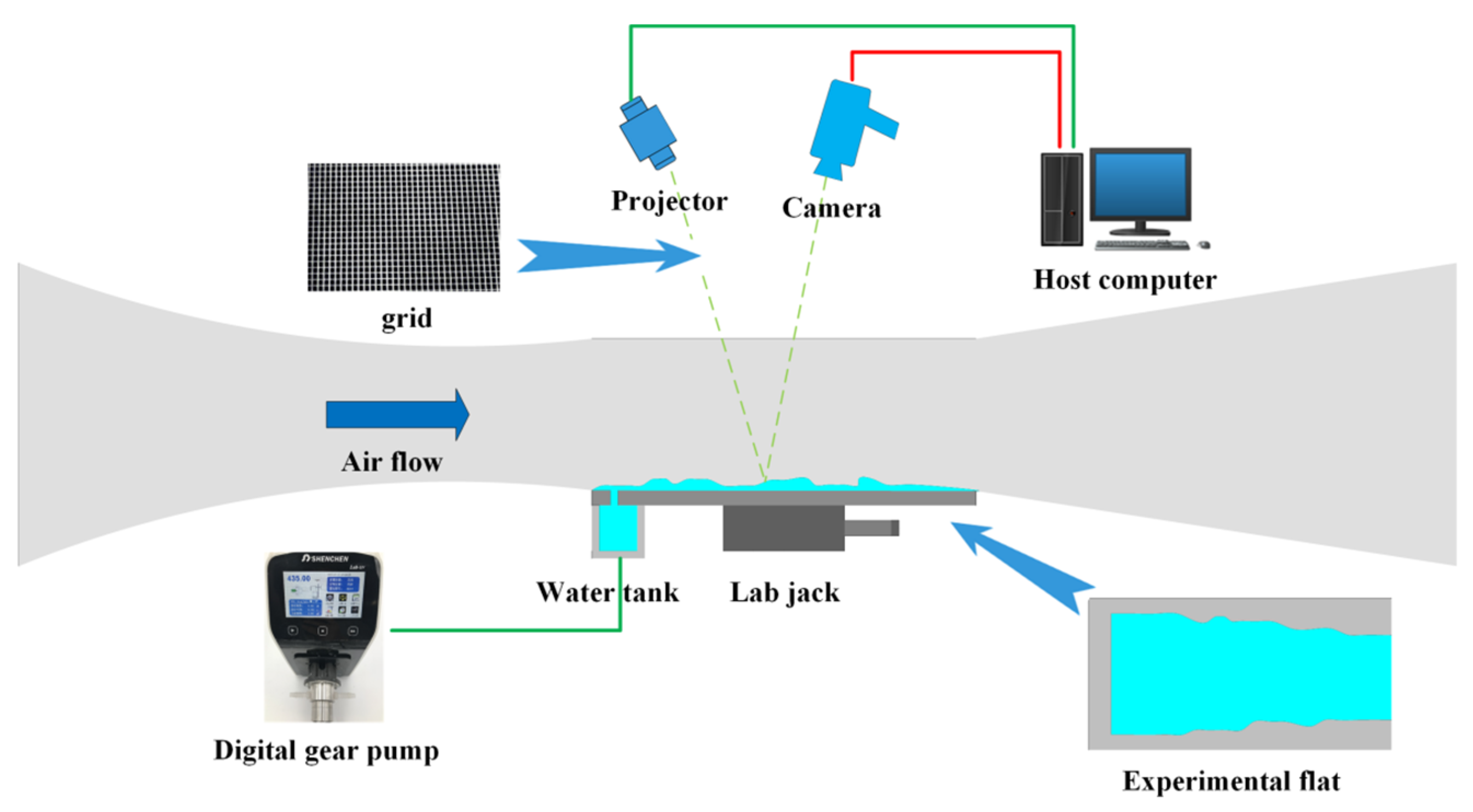
2.1. Experimental System

In this paper, an open water film wind tunnel experimental system was designed. The schematic diagram of the basic principle is shown in Figure 1. The main body comprised the contraction section, test section, and expansion section. High-speed airflow was provided by an axial fan downstream of the expansion section. Honeycombs and resistance nets were installed upstream of the contraction section to ensure the uniformity of airflow. The cross-section of the test section was 300 × 75 mm2, and the test structure was installed at the bottom. The front groove of the surface was a water outlet, and the bottom was connected with a water supply tank. A precision gear pump provided steady flow with a flow range of 57–1700 mL/min. A small amount of white latex paint was added to water to enhance the diffuse reflection of the water film surface. In the upper space of the test section, the projector was used to project the grid image, and the CCD camera was used for image acquisition at a frequency of 100 Hz.

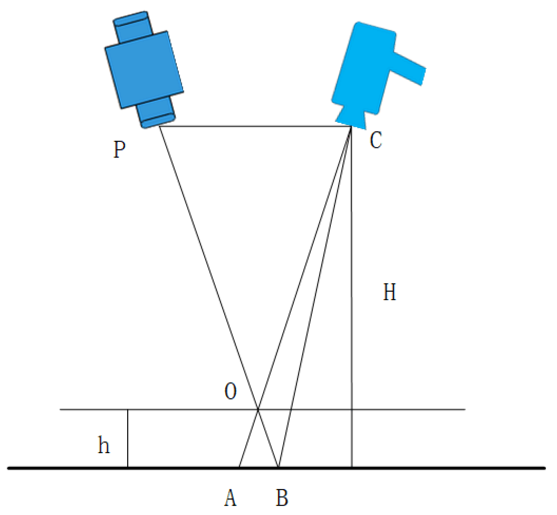
2.2. Measurement Principle of DIP System

The optical principle of DIP system is shown in Figure 2. The height of the reference plane was first set to 0. At this point, the grid image was projected to point B by the projector, captured by the camera, and recorded as a reference image. When the plane was elevated to a height h, the projector projected to the position of point O and recorded the experimental image. As the projector and the camera remained fixed, the range of view that the camera could take was also fixed. The position of the image pixels recorded by the camera indicated that the position of the point O in the experimental image was the same as that of point A in the original reference image. Therefore, compared with the reference image, the transverse displacement of the experimental image is A B ¯ when the height increased to h.
Figure 2 shows that the height of the camera from the reference plane was H. The camera lens C was taken as the origin, and the plane was parallel to the reference plane. Obviously, ΔABO was similar to ΔCPO, therefore:
h H h = A B ¯ C P ¯ ,
As Hh, the aforementioned equation can be simplified to:
h = H h C P ¯ A B ¯     H C P ¯ A B ¯ = K A B ¯ ,
Obviously, for a given optical system, H and C P ¯   are constant values. Therefore, the height displacement conversion coefficient K is a constant expressed in mm/pixel.
According to the principle of height displacement conversion, the thickness of the water film can be converted into the pixel displacement of the experimental and reference image. For the projection grid used in this experiment, the intersection point of a cross bright band of reference image was taken as the center point R(xr,yr), where xr is the transverse coordinate of the reference image pixel R, and yr is the longitudinal coordinate of the reference image pixel R. A search window (m,n) was set up, where m is the number of horizontal pixels and n is the number of vertical pixels. The same search window (m,n) was used to search the experimental image. First, the pixel center point E(xr,yr) of the same position of the experimental image was obtained. As the experimental image had a pixel shift compared with the reference image, it was obvious that the image in the search frame was different from the original reference image. The similarity between the two images was measured by introducing the correlation coefficient r, defined as:
r = m n ( R m n   R ¯   ) ( E m n   E ¯   ) ( m n ( R m n   R ¯   ) 2 ) ( m n ( E m n   E ¯   ) 2 ) ,
If r is closer to 1, the Rmn image is similar to Emn. Conversely, the closer r is to 0, the smaller the similarity between Rmn and Emn. In the case where the search window (m,n) remained unchanged, the pixel center point E moved, and the moving range was (i,j), where i is the number of horizontal pixels and j is the number of vertical pixels. In this way, the correlation coefficient r between the search window and the reference image window, and the correlation coefficient matrix r(i,j), could be obtained when the center point was at any point in E(xr,yr). Obviously, the peak of the correlation coefficient matrix was the center point E(xe,ye) of the experimental image. The displacement vector can be obtained by comparing the center point of the original reference image. The pixel difference obtained this time was an integer. To further improve the accuracy and achieve sub-pixel accuracy, the correlation coefficient matrix r(i,j) was fitted by quadratic polynomial near the center of the obtained experimental image. The peak value of the fitting function is obtained, which was the displacement vector (Δxy) with sub-pixel accuracy.

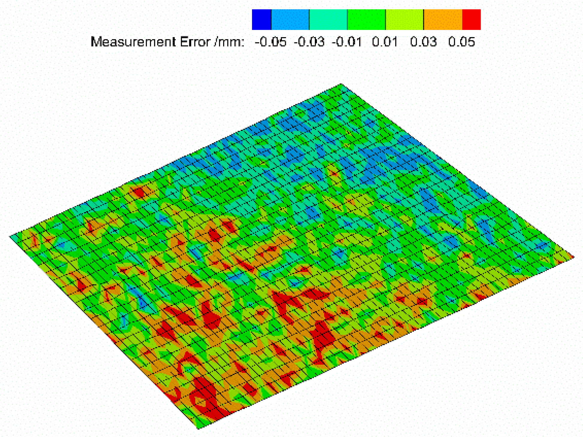
2.3. Experiment Bench Calibration and Measurement

Calibration was required before officially starting the experiments. As described in Section 2.2, the water film thickness can be converted into a lateral displacement in a specific direction. In this study, a cross-shaped grid was used. The measurement accuracy could be improved by keeping the lateral displacement direction the same as one of the cross-shaped grids when adjusting the test bench. After fixing the test bench, its height coordinate conversion coefficient K had a fixed value, and the K value was obtained, that is, the calibration of the test bench was completed.
The height of the adjusted test bed was set to z = 0 origin, and the reference image was taken. A precision-lifting platform was used to move up to eight parallel positions at 0.5mm intervals, and a grid image was taken at each position. All images were processed uniformly, and the displacement vector of each image under sub-pixel precision was obtained, which was compared with the height displacement of each image. Fitting the first-order function, the K value of the global grid of the test bed in this experiment is obtained, and the calibration was completed.
The bench was restored to z = 0 origin and a reference image was taken as shown in Figure 3a. The water film experiment was started using a high-speed camera and sampling at 100 Hz, and the experimental image was taken as shown in Figure 3b. Obviously, the surface mesh of the water film underwent significant bending and displacement. The displacement vectors of the experimental grid nodes were extracted and multiplied by local conversion constants to calculate the local water film thickness, and then the global water film thickness distribution was obtained.
The system was used to measure the plate height so as to evaluate the accuracy of the calibrated DIP system. The plate with a known thickness of 500 μm was placed on the experimental platform, and the experimental measurements were carried out according to the aforementioned steps. According to the measured results, the average thickness of the water film was 502.97 μm. Compared with the measurement range of this experiment, this error range in Figure 4 could meet the measurement accuracy requirements.

2.4. Rough Experimental Plate Setup

The rough test plates used in this paper were prepared by sandblasting the rough surface. Small particles of black corundum of different diameters were uniformly sprayed on the surface of the aluminum slab to simulate surface roughness. Therefore, the bottom of roughness is selected for the position of reference plane. The roughness value was measured with a roughness tester. Four test plates with different roughness were prepared in this experiment. The measurement results of roughness are shown in Table 1. The plates with different roughness were respectively installed on the water film test table, and water film flow tests was performed using the DIP water film measurement method, and the measurement results were analyzed.

3. Results and Analysis

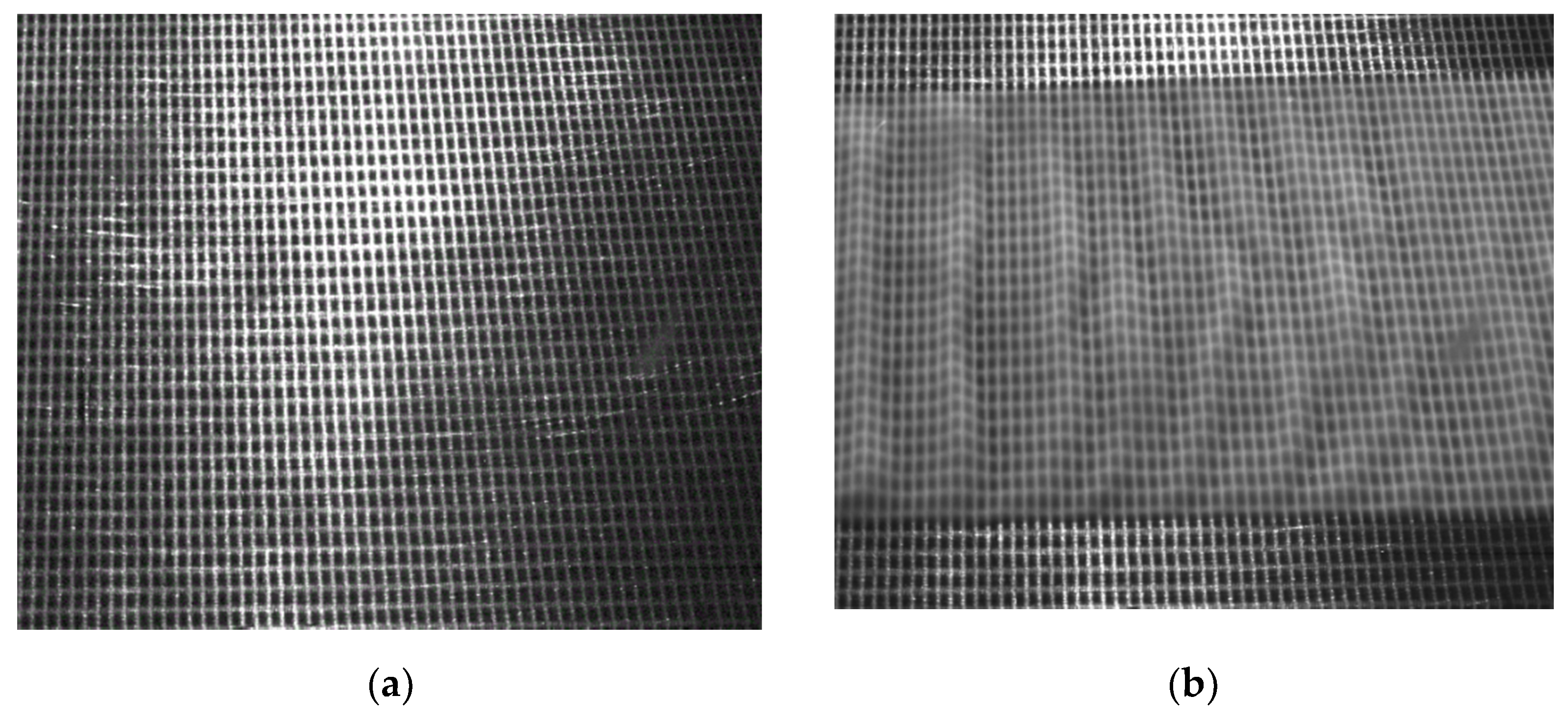
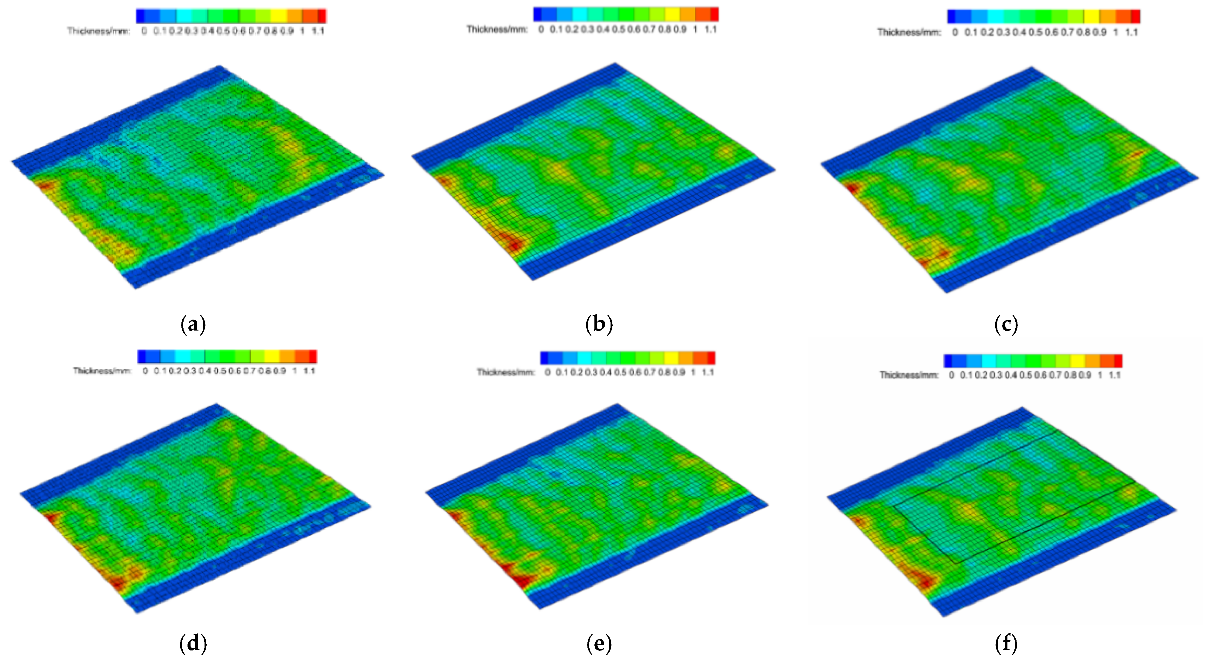
3.1. Water Film Measurement Processing Method

It was necessary to take the average of the thickness of the water film at different times to restrain the influence of fluctuation and randomness of water film on the experimental results. As shown in Figure 5a–e, the shooting results were taken every 0.2 s from t = 0 s to t = 0.8 s. The figure clearly shows that since the front end of the shooting was close to the water outlet, the thickness and fluctuation intensity of the water film were significantly larger than the overall average. Therefore, taking the middle and rear parts and avoiding the data on both sides of the experiment, using such a measurement sampling range was more in line with the actual situation. The actual sampling range is shown in Figure 5f.
For the grid area of measuring range a · b , the average thickness   δ ¯ of the water film was introduced, which was defined as:
  δ ¯ = 1 a · b q 1 b p 1 a δ p q ,
where a and b are the total number of grid points of the horizontal and vertical coordinates of the selected grid area, respectively; δ p q is the thickness of the local water film at the grid point (p,q); and   δ ¯ is the average of the thickness of the water film in the selected grid area. The average thickness of the water film under this condition could be obtained by calculating the thickness   δ ¯ of the water film five times and then averaging the treatment.

3.2. Water Film Flow Equation

In order to measure the flow rate of water film, dimensionless parameters are introduced. Reynolds number of water film, R e f is defined as:
R e f = Q / ( L · v l ) ,
where Q is the volume flow rate, L is the wetting width of the water film and v l is the kinematic viscosity of the liquid.
Aiming at addressing the problem of flat water film flow, Myers et al. [20,21] theoretically derived the prediction formula for continuous water film thickness. For the problem in this article, it can be simplified into a two-dimensional water film flow equilibrium height formula:
2   ρ l   g   s i n α h 3 +   3   τ h 2 = 6   μ l Q ,
where ρ l is liquid film density, g is gravitational acceleration,   μ l is liquid viscosity, Q is fluid flow per unit width.
In this experiment, for the water film flow problem of the horizontal plate, α = 0, the water film thickness h is equivalent to the average thickness of the water film   δ ¯ , that is:
  δ ¯ = h =   2   μ l Q τ ,
From the above formula, it can be obtained that the stable thickness h of the liquid film is only related to the viscosity of the liquid film   μ l , the liquid flow rate per unit width Q, and the shear force of the gas-liquid surface τ. In the water film test under the condition that the test temperature does not change, for a certain homogeneous fluid, the liquid film viscosity is constant, and the liquid flow rate per unit width can also be obtained directly. Only the airflow shear force τ is required to obtain the average thickness h of the water film, and the airflow shear force τ can be described as:
τ = f i 1 2 ρ a ( U a C ) 2 ,
where   f i is the interfacial shear factor, U a is the air velocity, ρ a is the air density, C is the phase velocity of gas-liquid interface wave. In the water film flow tests, due to the fact that U a >> C, the airflow shear force τ can be simplified as:
τ = f i 1 2 ρ a U a 2 ,
It can be seen that the only factor that determines the shear force τ of the airflow is the interfacial shear factor f i . We can predict the average thickness of the water film   δ ¯ through obtained f i   model.

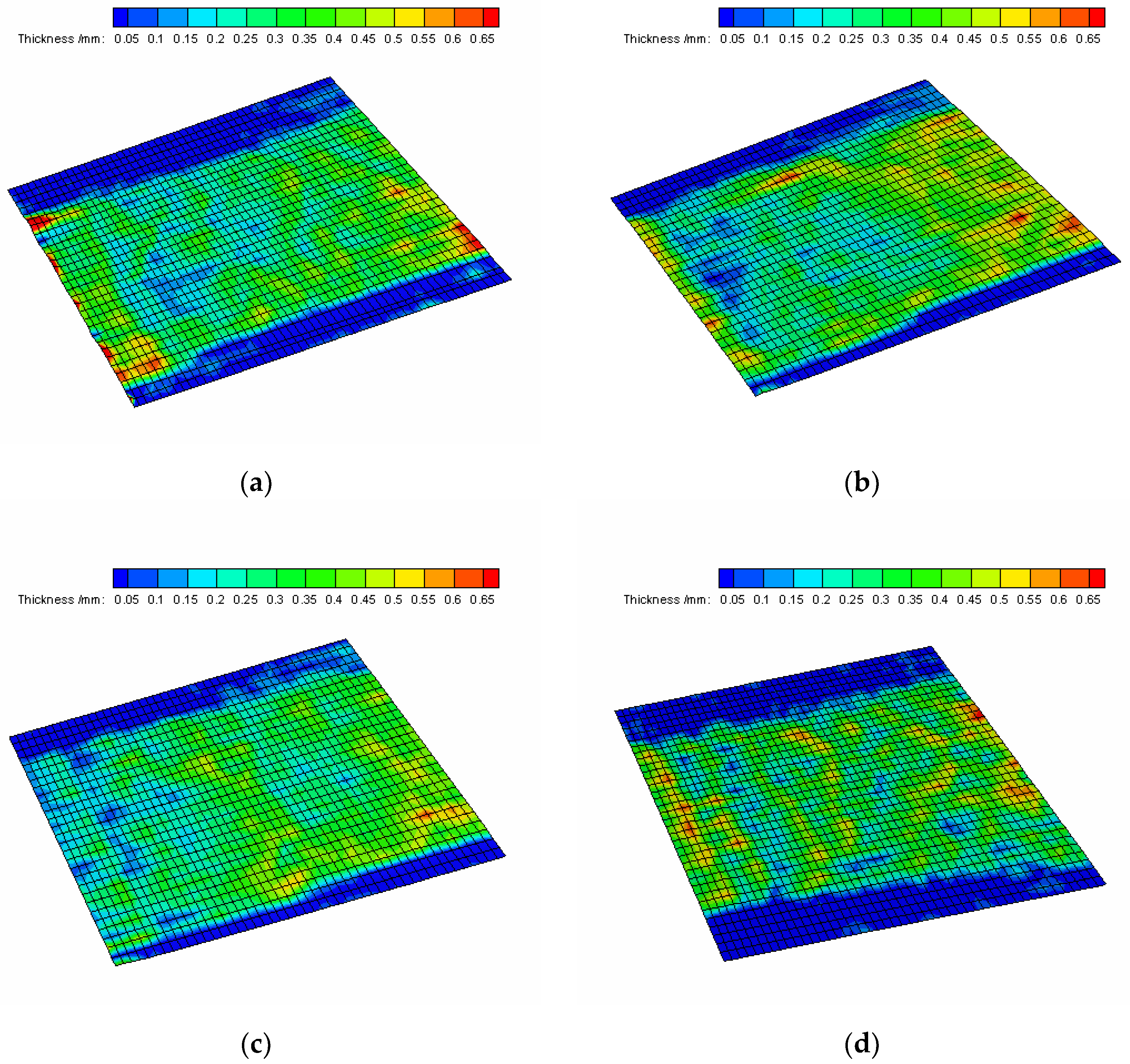
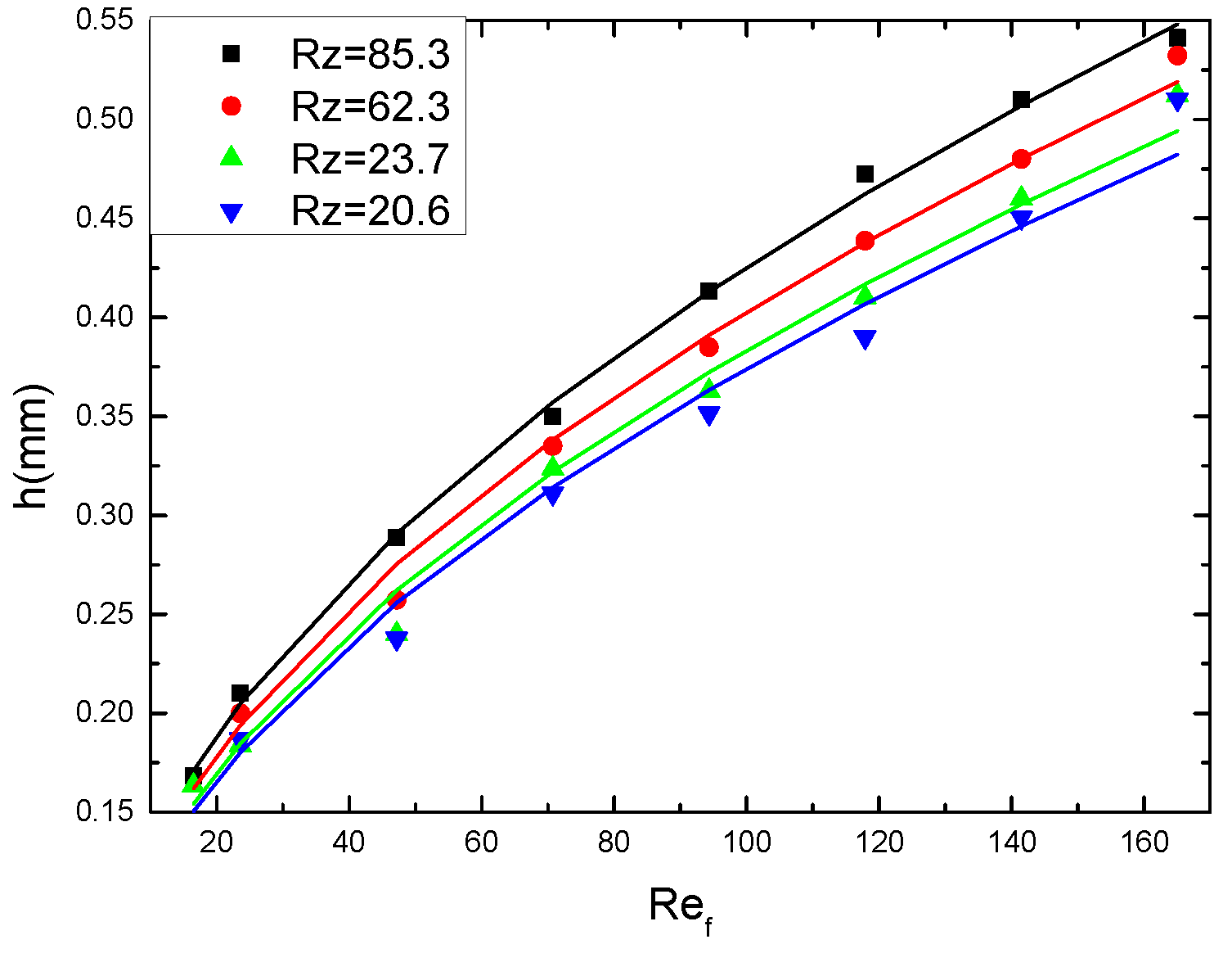
3.3. Effect of Roughness on Water Film Flow

In order to investigate the effect of roughness on the water film flow, a controlled variable method was used, the set speed was kept constant at 25 m/s, and the water flow speed was constant. The DIP measurement results and test images under different roughness conditions are shown in Figure 6. It can be seen from the figures that the flow state of the water film is very similar in the four groups of different roughness. The tested thickness of the water film is higher than the maximum contour height Rz of the surface roughness, and the minimum water film thickness can be less than 50 μm. When R e f is 25, the ratio of water film thickness to roughness changes from 2 to 8 with the increase of roughness. With the increase of R e f , the ratio of water film thickness to roughness increases gradually. When R e f increases to 160, the ratio of water film thickness to roughness is in the range of 6 to 25. During the water film flow, the rough elements of the flat plate are completely covered by the water film. The rough solid-liquid surface increases the frictional resistance of the water film flow. Furthermore, the grain structures of the rough surface will induce the water film flow to generate fine separation vortexes and dissipate the flow. These factors cause the average water film thickness under the same air speed and flow speed to increase as the surface roughness increases.
It is worth noting that an increase in roughness reduces the contact angle of water, according to the wetting theory. Therefore, in the stationary state, when the same amount of water adheres to flat plates with different roughness, the liquid film height will decrease as the roughness increases. Under constant wind driving and a constant water film flow, the factors that dominate the thickness of the liquid film are the gas-liquid surface shear force and the flow loss caused by the rough solid-liquid surface, and the surface contact angle of the liquid film is not a dominant factor in water film thickness. The conclusion obtained is contrary to the conclusion in the static state, and the thickness of the liquid film will increase as the surface roughness increases.
According to the water film Reynolds number formula, R e f = Q / ( L · v l ) = ( Q · ρ l ) / ( L · μ l ) was brought into the water film thickness formula and the airflow shear force formula to obtain the relationship between the interface shear coefficient and the water film thickness are as follows:
  f i = 4 μ l   R e f   L   δ ¯ 2 ρ l   ρ a U a 2 ,
It can be known from the above formula that, for a constant air velocity U a , the interface shear coefficient f i   is a function of the water film average thickness   δ ¯ and the water film Reynolds number R e f .
The relationship between the water film Reynolds number and the water film average thickness under different roughness determined in this paper is shown in Figure 7. It can be seen that the water film Reynolds number R e f can be regarded as function of the water film average thickness under the condition of constant air speed. The relational formula can be obtained by formula fitting, and the fitting formula of the interface shear coefficient f i can be obtained by substituting into Equation (10).
The interface shear coefficient relationship obtained f i by numerical fitting is shown in Table 2. For the function, its exponential power is unchanged, and the constant term is changed to adapt to different fitting curves.
It can be seen from the above equation that the interface shear coefficient f i and roughness Rz show a linear change. Taking the dimensionless factor CR = Rz/L, and then:
  f i = ( 0 . 822 ·   C R + 0 . 0039 ) ·   R e f 0 . 1144 ,
Let f i 0 be the interface shear coefficient of the smooth surface and f i R be the interface shear coefficient of the rough surface, then:
  f i R   = ( 1 210 . 77   ·   C R ) ·   f i 0 ,
Let the shearing force correction factor be C f i = ( 1 210 . 77 )   ·   C R , and substitute it into Equation (9) to obtain:
  τ r   =   C f i   ·   τ ,
where   τ r is the interfacial shear force of the rough surface.
Based on the analysis of the above results, for the problem of water film flow driven by wind, the surface roughness of the plate will change the friction resistance of the water film flow and induce the water film flow to generate vortex structures and lead to energy dissipation. These factors directly change the average thickness of the water film flow, but it is difficult to directly simulate the influence of roughness on water film flow. In the calculation, the flow state of smooth surface can be directly simulated. After the surface shear force is obtained, the influence of roughness on water film flow is directly embedded into the surface shear force to obtain the modified surface shear force. Using the modified surface shear force to calculate the water film flow process, the influence of roughness on the water film flow is considered.

4. Conclusions

In the numerical simulation of aircraft icing, the influence of roughness on heat transfer is usually considered, while the influence of surface roughness on flow is ignored. In this paper, a series of water film experiments were performed on different roughness surfaces using a developed DIP system. According to the results, the water film thickness increased with the increase of roughness. An innovative method for interfacial shear correction was proposed, and the effect of roughness on water film flow was embedded in interfacial shear force. The influence of roughness on water film flow is simulated by modifying the interface shear force, which provides some help for ice numerical simulation.

Author Contributions

Conceptualization, H.Z., C.Z. (Chunling Zhu), N.Z., C.Z. (Chengxiang Zhu) and Z.W.; methodology, C.Z. (Chunling Zhu), N.Z. and C.Z. (Chengxiang Zhu); validation, H.Z.; formal analysis, H.Z.; resources, C.Z. (Chunling Zhu); data curation, H.Z.; writing—original draft preparation, H.Z.; writing—review and editing, Z.W.; project administration, C.Z. (Chunling Zhu); funding acquisition, C.Z. (Chunling Zhu) and Z.W. All authors have read and agreed to the published version of the manuscript.

Funding

This research was funded by the National Natural Science Foundation of China (Grant No. 11832012, 51806105), the Natural Science Foundation of Jiangsu Province (Grant No. BK20180442) and Open Fund of Rotor Aerodynamics Key Laboratory (Grant No. RAL20190401).

Institutional Review Board Statement

Not applicable.

Informed Consent Statement

Not applicable.

Data Availability Statement

The data presented in this study are available on request from the corresponding author.

Conflicts of Interest

The authors declare no conflict of interest.

References

  1. Parent, O.; Ilinca, A. Anti-icing and De-icing Techniques for Wind turbines: Critical Review. Cold Reg. Sci. Technol. 2010, 65, 88–96. [Google Scholar] [CrossRef]
  2. Gent, R.W.; Dart, N.P.; Cansdale, J.T. Aircraft Icing. Philos. Trans. R. Soc. A Math. Phys. Eng. Sci. 2000, 358, 2873–2911. [Google Scholar] [CrossRef]
  3. Holl, M.; Patek, Z.; Smrcek, L. Wind Tunnel Testing of Performance Degradation of Ice Contaminated Airfoils. In Proceedings of the 22nd International Congress of Aeronautical Sciences, Harrogate, UK, 27 August–1 September 2000. [Google Scholar]
  4. Otta, S.P.; Rothmayer, A.P. Instability of Stagnation Line Icing. Comput. Fluids 2009, 38, 273–283. [Google Scholar] [CrossRef]
  5. Du, Y.; Gui, Y.; Xiao, C.; Xian, Y. Investigation on heat transfer characteristics of aircraft icing including runback water. Int. J. Heat Mass Transf. 2010, 53, 3702–3707. [Google Scholar]
  6. Zhang, X.; Wu, X.; Min, J. Aircraft icing model considering both rime ice property variability and runback water effect. Int. J. Heat Mass Transf. 2017, 104, 510–516. [Google Scholar] [CrossRef]
  7. Rothmayer, A.P.; Matheis, B.D.; Timoshin, S.N. Thin Liquid Films Flowing Over External Aerodynamics Surfaces. J. Eng. Math. 2002, 42, 341–357. [Google Scholar] [CrossRef]
  8. Rothmayer, A.P.; Hu, H. Linearized Solutions of Three-Dimensional Condensed Layer Films. In Proceedings of the 5th AIAA Atmospheric and Space Environments Conference, AIAA, San Diego, CA, USA, 24 June 2013. [Google Scholar]
  9. Wang, G.; Rothmayer, A.P. Thin Water Films Driven by Air Shear Stress through Roughness. Comput. Fluid 2009, 38, 235–246. [Google Scholar] [CrossRef]
  10. Shin, J.; Berkowitz, B. Prediction of Ice Shapes and Their Effect on Airfoil Drag. J. Aircr. 1994, 31, 263–270. [Google Scholar] [CrossRef]
  11. Wang, G. Thin Water Films Driven by Air through Surface Roughness. Ph.D. Thesis, Iowa State University, Ames, IA, USA, 2008. [Google Scholar]
  12. Wang, G.; Rothmayer, A.P. Air Driven Water Flow Past Small Scale Roughness. In Proceedings of the 43rd AIAA Aerospace Sciences Meeting and Exhibit, Reno, Nevada, 10 January–13 January 2005. [Google Scholar]
  13. Zhang, K.; Blake, J.; Alric, R.; Hu, H. An Experimental Investigation on Wind-Driven Rivulet/Film Flows over a NACA0012 Airfoil by Using Digital Image Projection Technique. In Proceedings of the 52nd Aerospace Sciences Meeting, AIAA, National Harbor, MD, USA, 13–17 January 2014. [Google Scholar]
  14. Cherdantsev, A.V.; Hann, D.B.; Azzopardi, B.J. Study of Gas-Sheared Liquid Film in Horizontal Rectangular Duct Using High-Speed LIF Technique: Three-Dimensional Wavy Structure and Its Relation to Liquid Entrainment. Int. J. Multiph. Flow 2014, 67, 52–64. [Google Scholar] [CrossRef]
  15. Zhang, K.; Zhang, S.; Rothmayer, A.P.; Hu, H. Development of a Digital Image Projection Technique to Measure Wind-Driven Water Film Flows. In Proceedings of the 51st AIAA Aerospace SCIENCES Meeting, Grapevine, TX, USA, 7–10 January 2013. [Google Scholar]
  16. Zhang, K.; Wei, T.; Hu, H. An Experimental Investigation on the Surface Water Transport Process over an Airfoil by Using a Digital Image Projection Technique. Exp. Fluids 2015, 56, 1–16. [Google Scholar] [CrossRef]
  17. Zhang, K.; Rothmayer, A.P.; Hu, H. An Experimental Study of Wind-Driven Water Film Flows over Roughness Array. In Proceedings of the 6th AIAA Atmospheric and Space Environments Conference, Atlanta, GA, USA, 16–20 June 2014. [Google Scholar]
  18. Chang, S.; Yu, W.; Song, M.; Leng, M.; Shi, Q. Investigation on Wavy Characteristics of Shear-Driven Water Film Using the Planar Laser Induced Fluorescence Method. Int. J. Multiph. Flow 2019, 118, 242–253. [Google Scholar]
  19. Leng, M.; Chang, S.; Wu, H. Experimental Investigation of Shear-Driven Water Film Flows on Horizontal Metal Plate. Exp. Therm. Fluid Sci. 2018, 94, 134–147. [Google Scholar] [CrossRef] [Green Version]
  20. Myers, T.G.; Thompson, C.P. Modeling the Flow of Water on Aircraft in Icing Conditions. AIAA J. 1998, 36, 1010–1013. [Google Scholar] [CrossRef]
  21. Myers, T.G.; Charpin, J.P.; Thompson, C.P. Slowly Accreting Ice Due to Supercooled Water Impacting on a Cold Surface. Phys. Fluids 2002, 14, 240. [Google Scholar] [CrossRef]
Figure 1. Water film experimental system.
Aerospace 08 00225 g001
Figure 2. Optical principle of height position conversion.
Aerospace 08 00225 g002
Figure 3. Typical experimental state image: (a) Reference image; (b) Experimental image.
Aerospace 08 00225 g003
Figure 4. Measurement system error range.
Aerospace 08 00225 g004
Figure 5. Instantaneous image and data processing range: (a) t = 0 s; (b) t = 0.2 s; (c) t = 0.4 s; (d) t = 0.6 s; (e) t = 0.8 s; (f) Data processing range.
Aerospace 08 00225 g005
Figure 6. DIP measurement results under different roughness: (a) Rz = 20.6 μm; (b) Rz = 23.7 μm; (c) Rz = 62.3 μm; (d) Rz = 85.3 μm.
Aerospace 08 00225 g006
Figure 7. Comparison of average thickness of water film under different roughness.
Aerospace 08 00225 g007
Table 1. Surface roughness of water film test plates.
NumberRa/μmRz/μm
12.820.6
23.323.7
38.762.3
413.985.3
Table 2. Relational formula of interface shear coefficient under different roughness.
Rz/μmFunction
20.6 f i = 0 . 003734   ·   R e f 0 . 1144
23.7 f i = 0 . 003556   ·   R e f 0 . 1144
62.3 f i = 0 . 003224   ·   R e f 0 . 1144
85.3 f i = 0 . 00289   ·   R e f 0 . 1144
Publisher’s Note: MDPI stays neutral with regard to jurisdictional claims in published maps and institutional affiliations.

