A Comparison of Closed-Loop Performance of Multirotor Configurations Using Non-Linear Dynamic Inversion Control

Abstract

Multirotor is the umbrella term for the family of unmanned aircraft, which include the quadrotor, hexarotor and other vertical take-off and landing (VTOL) aircraft that employ multiple main rotors for lift and control. Development and testing of novel multirotor designs has been aided by the proliferation of 3D printing and inexpensive flight controllers and components. Different multirotor configurations exhibit specific strengths, while presenting unique challenges with regards to design and control. This article highlights the primary differences between three multirotor platforms: a quadrotor; a fully-actuated hexarotor; and an octorotor. Each platform is modelled and then controlled using non-linear dynamic inversion. The differences in dynamics, control and performance are then discussed.

1. Introduction

A multirotor is a rotorcraft, but differ from traditional helicopter configurations. Rather than employing mechanically-complex main and tail rotors, a multirotor employs several identical rotors to provide both lift and control. The flexibility of the platform has led to the popular application as an unmanned aerial vehicle (UAV). A prominent example of this is the quadrotor, which has seen popular use in research, commercial and hobby applications. The primary benefit of the quadrotor lies in its mechanical simplicity: its lifting force and controlling moments are supplied exclusively through manipulation of the four fixed-pitch rotors.

Additional multirotor platforms are easily conceived by augmenting the quadrotor with additional rotors. This provides greater lifting force without the need to upgrade components, such as the rotor blades and motors. However, the introduction of additional rotors changes the dynamic performance of the system, adding extra mass and typically requiring additional supporting structure.

Naturally, the change in dynamics affects the requirements of the multirotor’s control system. Either the controller gains remain consistent with each platform and the closed-loop response changes or the controller must be updated with each configuration to achieve comparable system performance. The notion of achieving a consistent closed-loop response in different systems is realised through the use of non-linear dynamic inversion (NDI) [1], also known as feedback linearisation, whereby the dynamics of a relatively simple system are mathematically inverted, such that the system dynamics are linearised in a closed loop. The primary benefit of this approach in the context of obtaining consistent system performance across a range of platforms is that it transforms a non-linear multiple-input multiple-output (MIMO) system into a series of linear single-input single-output (SISO) systems. The performances of these linear systems are then specified through simple pole placement or, if desired, more complex control laws [2]. Thus, a consistent closed-loop dynamic performance may specified across a range of multirotor systems.

This paper presents a comparison of three specific multirotor platforms: quadrotor, hexarotor and octorotor. Taking the quadrotor as the baseline system, a discussion is presented on the changes to the vehicle dynamics, controller and closed-loop performance as a result of augmenting the aircraft with additional rotors. The common properties of the vehicles are first presented. The differences in each configuration are then described. The dynamic model of each vehicle enables the definition of a unique feedback, which results in a linear, second-order system in a closed loop. Specifying a standard state-feedback control law for each multirotor system, the closed-loop performance of each vehicle is harmonised. It is seen through simulation testing that the actuator limits in each system limit the ability of each system to exhibit identical performance.

Figure 1. A quadrotor micro air vehicle.

Figure 1. A quadrotor micro air vehicle.

2. Review of the Literature

The mechanical simplicity of multirotors, such as the quadrotor, has made it a popular fixture in academic literature. In particular, the dynamic qualities of the quadrotor make it an ideal test bed for the investigation of non-linear control methods. This section describes highlights from the literature relating to multirotor vehicles. Application of NDI to multirotor vehicles is also described.

2.1. Multirotor Platforms

Modelling, control and application of the quadrotor vehicle is prominent in the literature. Research applications include detailed simulation [3], trajectory generation [4,5,6], multi-resolution modelling experiments [1,7] and control design [8,9,10]. Such investigations primarily focus on the quadrotor over alternative multirotor configurations. The foremost argument for this is the simplicity of the resulting system dynamics, which lack the the servo-controlled thrust vectoring required by trirotor configurations [11] or the additional rotors of pentarotors, hexarotors, etc.

However limited in comparison to the quadrotor, research employing more novel multirotor configurations does exist in the literature, as evidenced by the trirotor described by [11], the LQRhexarotor controller of [12], the co-axial hexarotor in [13], the fully-actuated hexarotor of [14] and the octorotor described in [15]. As with the quadrotor, applications of the various platforms range from simple control investigation to state estimation to fault tolerant control strategies. While these investigations are indicative of those performed on the quadrotor, the literature highlights a lack of discussion on the differences of multirotor platforms with regards to such investigations.

2.2. NDI Control of Multirotors

Non-linear dynamic inversion control, or feedback linearisation control, is a non-linear control strategy with popular application to the quadrotor, as in [2,8,16]. As NDI requires the dynamics of the system to be invertible, the simplicity of the quadrotor lends itself well to NDI control. Application to other multirotor platforms is less well documented, but an instance of its use on a hexarotor is described in [17].

Comparison of NDI control to the ubiquitous PID (proportional integral derivative) method has demonstrated the superior response characteristics of the former approach [1]. The primary downside of NDI is the amount of information required about the system in order to produce an optimal response.

3. Multirotor Dynamics

In order to synthesise a dynamic inversion controller for each platform, the dynamic models in each case must be considered. While the three configurations differ in layout and quantity of rotors, they also have several common properties. The structure of each system may therefore be considered a combination of a number of shared properties and a few platform-specific qualities.

3.1. Shared Properties

Each multirotor configuration may be modelled as a six degrees of freedom rigid body. Assuming a simple linear rotor model, the force and moment contributions to the rigid body response arise exclusively from gravitational acceleration and rotor thrust and torque. Common rigid body and rotor models may then be used for all multirotor systems. Then, it is simply the number of rotors, and thus, the composition of the net force and moment vectors that change between systems.

3.1.1. Rigid Body Model

The rigid body model of each multirotor system is derived using Euler–Lagrange formalism, as described in [1]. If $\mathbf{T}$ and $\mathbf{M}$ are respectively the force and moment vectors arising purely from rotor thrust and torque contribution, the general rigid body model is then:

$$\begin{array}{cc}\hfill \ddot{\mathbf{r}}& =\frac{1}{m}{\mathbf{R}}_{\mathcal{B}}^{\mathcal{W}}\mathbf{T}+g{\widehat{\mathbf{z}}}^{\mathcal{W}}\hfill \\ \hfill \ddot{\eta }& ={\mathbf{I}}^{-1}\mathbf{M}\hfill \end{array}$$

(1)

where $\mathbf{r}\in {\mathbf{R}}^3$ describes the position of the body in an inertially-fixed world frame $\mathcal{W}$ and $\eta \in {\mathbf{R}}^3$ is the vector of Euler angles relating the attitude of the body-fixed frame $\mathcal{B}$ to $\mathcal{W}$. The direction cosine matrix ${\mathbf{R}}_{\mathcal{B}}^{\mathcal{W}}$, relating the body-fixed frame to the world frame, is defined by:

$$\begin{array}{cc}\hfill {\mathbf{R}}_{\mathcal{W}}^{\mathcal{B}}& =\left[\begin{array}{ccc}{c}_{\theta }{c}_{\psi }& c_{\theta }{s}_{\psi }& -s_{\theta }\\ s_{\varphi }{s}_{\theta }{c}_{\psi }-c_{\varphi }{s}_{\psi }& s_{\varphi }{s}_{\theta }{s}_{\psi }+c_{\varphi }{c}_{\psi }& s_{\varphi }{c}_{\theta }\\ c_{\varphi }{s}_{\theta }{c}_{\psi }+s_{\varphi }{s}_{\psi }& c_{\varphi }{s}_{\theta }{s}_{\psi }-s_{\varphi }{c}_{\psi }& c_{\varphi }{c}_{\theta }\end{array}\right]\hfill \end{array}$$

(2)

$$\begin{array}{cc}\hfill {\mathbf{R}}_{\mathcal{B}}^{\mathcal{W}}& ={\left({\mathbf{R}}_{\mathcal{W}}^{\mathcal{B}}\right)}^T\hfill \end{array}$$

(3)

The system state then simply describes the displacement and velocity of the rigid body in each degree of freedom and is therefore:

$$\mathbf{x}={[x,y,z,\varphi ,\theta ,\psi ,\dot{x},\dot{y},\dot{z},\dot{\varphi },\dot{\theta },\dot{\psi }]}^T$$

The system output is similarly common to all configurations and is simply the displacement in each degree of freedom, or:

$$\mathbf{y}={[x,y,z,\varphi ,\theta ,\psi ]}^T$$

3.1.2. Rotor Model

While the number of rotors changes between platforms, the relationship between a rotor’s thrust and torque and its input is described by a model common to all systems. Consider a rotor driven by a constant battery voltage and a rotor speed-regulating pulse width modulation (PWM) signal. Linear relationships may be drawn between the thrust T, torque Q and zeroed PWM u of any rotor. For a single rotor i, these relationships are:

$$\begin{array}{ccccc}\hfill T_i& =K_T{u}_i\hfill & \hfill \hspace{1em}\hspace{1em}\hspace{1em}& \hfill Q_i& =K_Q{u}_i\hfill \end{array}$$

(4)

where $K_T$ and $K_Q$ are constant thrust and torque gains, respectively.

Thus, for each platform, a given number of rotors m implies an identical number of inputs:

$$\mathbf{u}={[u_1,u_2,\dots u_m]}^T$$

(5)

with a unique force and moment contribution to the rigid body model described by Equation (1), which depends on the position, orientation and number of rotors.

The net thrust vector of any multirotor is then obtained by summing the thrusts from each rotor, giving:

$$\mathbf{T}=\sum _{i=1}^m{T}_i{\widehat{\mathbf{n}}}_i$$

(6)

where ${\widehat{\mathbf{n}}}_i$ is the unit direction vector describing the axis of rotation of rotor i in $\mathcal{B}$. The net moment vector is similarly obtained by considering the moment arms of each rotor’s thrust vector and the torque of each rotor, giving:

$$\mathbf{M}=\sum _{i=1}^m{\mathbf{r}}_i^{\mathcal{B}}\times T_i{\widehat{\mathbf{n}}}_i+Q_i{\widehat{\mathbf{n}}}_i$$

(7)

where ${\mathbf{r}}_i^{\mathcal{B}}$ is the position of rotor i in $\mathcal{B}$.

3.1.3. General Model Description and Control Allocation

Each system can be considered control-affine, of the form:

$$\begin{array}{cc}\hfill \dot{\mathbf{x}}& =f\left(\mathbf{x}\right)+g\left(\mathbf{x}\right)\mathbf{u}\hfill \\ \hfill \mathbf{y}& =h\left(\mathbf{x}\right)\hfill \end{array}$$

(8)

such that the system dynamics are invertible, as described in Section 4. Additionally, the actuation of each system may be highlighted by a set of n pseudo-inputs ${\mathbf{u}}^{*}$, where n is the number of degrees of freedom, which are directly excitable. The pseudo-input vector is constructed by considering the non-zero elements of the thrust and moment vectors $\mathbf{T}$ and $\mathbf{M}$.

The pseudo-input vector is related to the true system input through a control matrix $\mathbf{C}$. This matrix is obtained from the Jacobian of the pseudo-input ${\mathbf{u}}^{*}\left(\mathbf{u}\right)$ with respect to the input $\mathbf{u}$, or:

$$\mathbf{C}=\frac{\partial {\mathbf{u}}^{*}\left(\mathbf{u}\right)}{\partial \mathbf{u}}$$

(9)

The resulting relationship:

$${\mathbf{u}}^{*}=\mathbf{C}\mathbf{u}$$

(10)

is invertible for any control matrix using the method described by [18]:

$$\mathbf{u}={\mathbf{C}}^{+}{\mathbf{u}}^{*},\text{where}{\mathbf{C}}^{+}={\mathbf{C}}^T{\left(\mathbf{C}{\mathbf{C}}^T\right)}^{-1}$$

(11)

where the pseudo-inverse ${\mathbf{C}}^{+}$ is defined as the control allocation matrix. For square matrices $\mathbf{C}$, the pseudo-inverse is simply the inverse ${\mathbf{C}}^{+}={\mathbf{C}}^{-1}$.

3.2. The Quadrotor

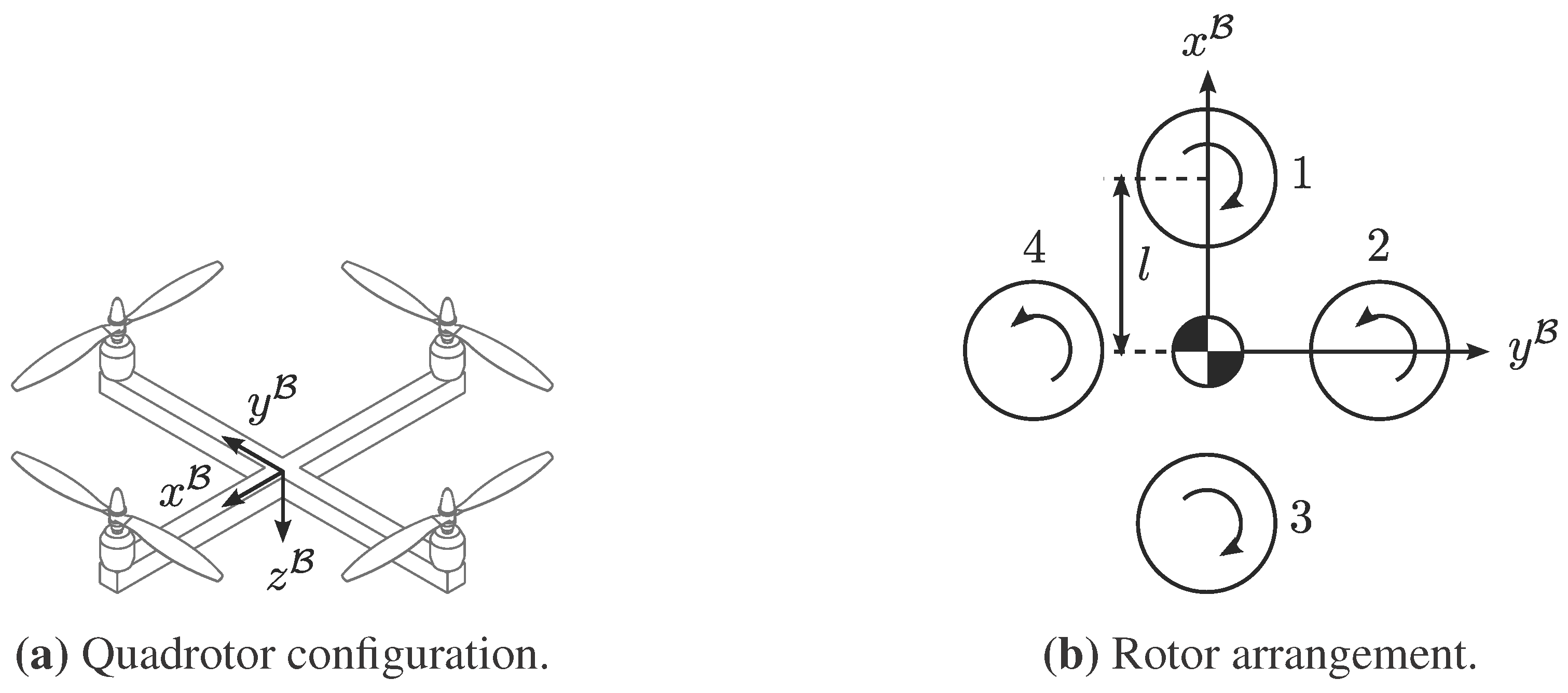
The quadrotor is a popular micro air vehicle platform, consisting of four rotors spaced equidistantly around the centre of mass. In the typical “cross” configuration, pitching motion is achieved by adjusting the thrust differential between the front and rear rotors. Rolling motion is similarly obtained by adjusting the thrust differential between the left and right rotors. Yawing motion is achieved by adjusting the net torque differential between all four rotors. Translational motion is induced by controlling the net thrust from the rotors and pitching and rolling the aircraft in the desired direction. The quadrotor has four inputs and six degrees of freedom and is therefore under-actuated.

The quadrotor axes’ definition and rotor arrangement are shown in Figure 2. In this case, Rotors 1 and 3 rotate clockwise, while Rotors 2 and 4 rotate counter-clockwise. As the axis of rotation of each rotor is aligned with the $z^{\mathcal{B}}$ axis, thrust and torque act exclusively in $z^{\mathcal{B}}$. The net thrust and moment vectors of the quadrotor are therefore respectively described by:

$$\begin{array}{ccccc}\hfill \mathbf{T}& =\left[\begin{array}{c}0\\ 0\\ -K_T\left(u_1+u_2+u_3+u_4\right)\end{array}\right]\hfill & \hfill \hspace{1em}\hspace{1em}\hspace{1em}& \hfill \mathbf{M}& =\left[\begin{array}{c}{K}_{T}l(u_4-u_2)\\ K_{T}l(u_1-u_3)\\ K_Q(-u_1+u_2-u_3+u_4)\end{array}\right]\hfill \end{array}$$

(12)

Figure 2. Quadrotor configuration and the axes’ definition.

Figure 2. Quadrotor configuration and the axes’ definition.

As the quadrotor is under-actuated, its thrust and moment vectors contain zero elements. The resulting four pseudo-inputs ${\mathbf{u}}^{*}$ are then chosen to be the non-zero elements of $\mathbf{T}$ and $\mathbf{M}$. They therefore may be described as functions of the true inputs $\mathbf{u}$ and the vehicle properties, giving:

$${\mathbf{u}}^{*}=\left[\begin{array}{c}{u}_z\\ u_{\varphi }\\ u_{\theta }\\ u_{\psi }\end{array}\right]=\left[\begin{array}{c}-K_T(u_1+u_2+u_3+u_4)\\ K_{T}l(u_4-u_1)\\ K_{T}l(u_1-u_3)\\ K_Q(-u_1+u_2-u_3+u_4)\end{array}\right]$$

(13)

The quadrotor’s control matrix $\mathbf{C}$ is thus obtained from Equation (9) and defined as:

$$\mathbf{C}=\left[\begin{array}{cccc}-K_T& -K_T& -K_T& -K_T\\ 0& -K_{T}l& 0& K_{T}l\\ K_{T}l& 0& -K_{T}l& 0\\ -K_Q& K_Q& -K_Q& K_Q\end{array}\right]$$

(14)

Thus, considering the general rigid body model described by Equation (1) and substituting the rotor inputs for the pseudo-inputs, the dynamic model of the quadrotor is described by:

$$\begin{array}{ccccc}\hfill \ddot{\mathbf{r}}& =\frac{1}{m}{\mathbf{R}}_{\mathcal{B}}^{\mathcal{W}}\left[\begin{array}{c}0\\ 0\\ u_z\end{array}\right]+\left[\begin{array}{c}0\\ 0\\ g\end{array}\right]\hfill & \hfill \hspace{1em}\hspace{1em}\hspace{1em}& \hfill \ddot{\eta }& ={\mathbf{I}}^{-1}\left[\begin{array}{c}{u}_{\varphi }\\ u_{\theta }\\ u_{\psi }\end{array}\right]\hfill \end{array}$$

(15)

where it is clear that the pseudo-inputs describe the force in a given body axis or the moment about a given axis.

3.3. The Hexarotor

The hexarotor platform described here is inspired by the Dot-HRdescribed by [14], where the rotational axes of the six rotors are inclined from the vertical axis. This introduces thrust components in the $x^{\mathcal{B}}$ and $y^{\mathcal{B}}$ axes of the vehicle and permits fully-actuated control of its six degrees of freedom. As with the quadrotor, roll, pitch and yaw moments may be induced by varying the thrust and torque differentials of the rotors.

The hexarotor axes’ definition and rotor arrangement are shown in Figure 3. The rotors are arranged in two layers, each layer composed of an equilateral triangle with three rotors. The upper layer sits above the centre of mass and has the rotors pointing towards the $z^{\mathcal{B}}$ axis. The lower layer sits below the centre of mass and has the rotors pointing outward from the $z^{\mathcal{B}}$ axis. Each rotor arm is inclined from the body x–y plane by an angle α, while the axis of rotation of each rotor is normal to that rotor’s arm. The thrust and torque vector of each rotor is therefore displaced from the $z^{\mathcal{B}}$ axis by α. The rotors are spaced equally around the centre of mass at increments of 60 and distance l. Further flexibility in the platform may be achieved by explicitly specifying a unique position and orientation for each rotor.

The net thrust and moment in $\mathcal{B}$ are obtained by summing the thrust and moments produced by each rotor, as in Equations (6) and (7). Due to the angular offset of each motor, both the net thrust and moment vectors have components in all three body axes. To simplify the moment vector, it is assumed that the net torque differential is sufficiently small with respect to the rolling and pitching moments that it has an impact only about the $z^{\mathcal{B}}$ axis. The thrust and torque vectors are therefore described by:

$$\begin{array}{cc}\hfill \mathbf{T}& =\left[\begin{array}{c}{K}_{T}sin\alpha \left(u_3+u_4-\frac{1}{2}(u_1+u_2+u_5+u_6)\right)\\ K_{T}sin\alpha \frac{\sqrt{3}}{2}\left(u_1-u_2+u_5-u_6\right)\\ -K_{T}cos\alpha \left(u_1+u_2+u_3+u_4+u_5+u_6\right)\end{array}\right]\hfill \\ \hfill \mathbf{M}& =\left[\begin{array}{c}{K}_{T}l\frac{\sqrt{3}}{2}\left(u_1-u_2-u_5+u_6\right)\\ K_{T}l\left(u_3-u_4-\frac{1}{2}(u_1+u_2-u_5-u_6)\right)\\ K_Q\left(-u_1-u_2-u_3+u_4+u_5+u_6\right)\end{array}\right]\hfill \end{array}$$

(16)

Figure 3. Hexarotor configuration and the axes’ definition.

Figure 3. Hexarotor configuration and the axes’ definition.

The hexarotor in this form is fully actuated. Its six pseudo-inputs may therefore be equated to the thrust and moment in each body axis. Describing the pseudo-inputs as functions of the true inputs $\mathbf{u}$ provides the relationship:

$$\begin{array}{c}\hfill {\mathbf{u}}^{*}=\left[\begin{array}{c}{u}_x\\ u_y\\ u_z\\ u_{\varphi }\\ u_{\theta }\\ u_{\psi }\end{array}\right]=\left[\begin{array}{c}{K}_{T}sin\alpha \left(u_3+u_4-\frac{1}{2}(u_1+u_2+u_5+u_6)\right)\\ K_{T}sin\alpha \frac{\sqrt{3}}{2}\left(u_1-u_2+u_5-u_6\right)\\ -K_{T}cos\alpha \left(u_1+u_2+u_3+u_4+u_5+u_6\right)\\ K_{T}l\frac{\sqrt{3}}{2}\left(u_1-u_2-u_5+u_6\right)\\ K_{T}l\left(u_3-u_4-\frac{1}{2}(u_1+u_2-u_5-u_6)\right)\\ K_Q\left(-u_1-u_2-u_3+u_4+u_5+u_6\right)\end{array}\right]\end{array}$$

and, from Equation (9), the resulting control matrix:

$$\mathbf{C}=\left[\begin{array}{cccccc}-\frac{1}{2}{K}_{T}sin\alpha & -\frac{1}{2}{K}_{T}sin\alpha & K_{T}sin\alpha & K_{T}sin\alpha & -\frac{1}{2}{K}_{T}sin\alpha & -\frac{1}{2}{K}_{T}sin\alpha \\ \frac{\sqrt{3}}{2}{K}_{T}sin\alpha & -\frac{\sqrt{3}}{2}{K}_{T}sin\alpha & 0& 0& \frac{\sqrt{3}}{2}{K}_{T}sin\alpha & -\frac{\sqrt{3}}{2}{K}_{T}sin\alpha \\ -K_{T}cos\alpha & -K_{T}cos\alpha & -K_{T}cos\alpha & -K_{T}cos\alpha & -K_{T}cos\alpha & -K_{T}cos\alpha \\ \frac{\sqrt{3}}{2}{K}_{T}l& -\frac{\sqrt{3}}{2}{K}_{T}l& 0& 0& -\frac{\sqrt{3}}{2}{K}_{T}l& \frac{\sqrt{3}}{2}{K}_{T}l\\ \frac{1}{2}{K}_{T}l& \frac{1}{2}{K}_{T}l& -K_{T}l& K_{T}l& -\frac{1}{2}{K}_{T}l& -\frac{1}{2}{K}_{T}l\\ -K_Q& -K_Q& -K_Q& K_Q& K_Q& K_Q\end{array}\right]$$

(17)

Then, considering Equation (1)’s rigid body model, the dynamic model of the hexarotor may be related to the pseudo-inputs by:

$$\begin{array}{ccccc}\hfill \ddot{\mathbf{r}}& =\frac{1}{m}{\mathbf{R}}_{\mathcal{B}}^{\mathcal{W}}\left[\begin{array}{c}{u}_x\\ u_y\\ u_z\end{array}\right]+\left[\begin{array}{c}0\\ 0\\ g\end{array}\right]\hfill & \hfill \hspace{1em}\hspace{1em}\hspace{1em}& \hfill \ddot{\eta }& ={\mathbf{I}}^{-1}\left[\begin{array}{c}{u}_{\varphi }\\ u_{\theta }\\ u_{\psi }\end{array}\right]\hfill \end{array}$$

(18)

3.4. The Octorotor

The octorotor is described as an extension of the quadrotor platform, with four additional rotors to provide greater thrust. As with the quadrotor, each of the rotors provides thrust only in the $-z^{\mathcal{B}}$ direction. Despite having a total of eight rotors, the octorotor is also under-actuated, as it can only directly excite motion in four of the vehicle’s six degrees of freedom.

The octorotor axes’ definition and rotor arrangement are shown in Figure 4. The rotors are arranged in an “H” configuration, with Rotors 1, 3, 6 and 8 rotating clockwise and Rotors 2, 4, 5 and 7 rotating counter-clockwise. Each rotor is displaced from the centre of mass in the $x^{\mathcal{B}}$ axis by a distance of either $l_{x1}$ or $l_{x2}$ and in the $y^{\mathcal{B}}$ axis by a distance $l_y$. The net thrust and moment vectors of the octorotor are obtained from Equations (6) and (7), giving:

$$\begin{array}{cc}\hfill \mathbf{T}& =\left[\begin{array}{c}0\\ 0\\ -K_T\left(u_1+u_2+u_3+u_4+u_5+u_6+u_7+u_8\right)\end{array}\right]\hfill \\ \hfill \mathbf{M}& =\left[\begin{array}{c}{K}_T{l}_y\left(u_1-u_2+u_3-u_4+u_5-u_6+u_7-u_8\right)\\ K_T\left(l_{x1}(u_3+u_4-u_5-u_6)+l_{x2}(u_1+u_2-u_7-u_8)\right)\\ K_Q\left(-u_1+u_2-u_3+u_4+u_5-u_6+u_7-u_8\right)\end{array}\right]\hfill \end{array}$$

(19)

Figure 4. Octorotor configuration and the axes’ definition.

Figure 4. Octorotor configuration and the axes’ definition.

The octorotor is under-actuated, and its net thrust vector contains the same zero elements as that of the quadrotor. The pseudo-input vector may therefore be similarly constructed as a function of the true inputs, giving:

$${\mathbf{u}}^{*}=\left[\begin{array}{c}{u}_z\\ u_{\varphi }\\ u_{\theta }\\ u_{\psi }\end{array}\right]=\left[\begin{array}{c}-K_T\left(u_1+u_2+u_3+u_4+u_5+u_6+u_7+u_8\right)\\ K_T{l}_y\left(u_1-u_2+u_3-u_4+u_5-u_6+u_7-u_8\right)\\ K_T\left(l_{x1}(u_3+u_4-u_5-u_6)+l_{x2}(u_1+u_2-u_7-u_8)\right)\\ K_Q\left(-u_1+u_2-u_3+u_4+u_5-u_6+u_7-u_8\right)\end{array}\right]$$

(20)

From Equation (9), the octorotor’s control matrix is then:

$$\mathbf{C}=\left[\begin{array}{cccccccc}-K_T& -K_T& -K_T& -K_T& -K_T& -K_T& -K_T& -K_T\\ K_T{l}_y& -K_T{l}_y& K_T{l}_y& -K_T{l}_y& K_T{l}_y& -K_T{l}_y& K_T{l}_y& -K_T{l}_y\\ K_T{l}_{x2}& K_T{l}_{x2}& K_T{l}_{x1}& K_T{l}_{x1}& -K_T{l}_{x1}& -K_T{l}_{x1}& -K_T{l}_{x2}& -K_T{l}_{x2}\\ -K_Q& K_Q& -K_Q& K_Q& K_Q& -K_Q& K_Q& -K_Q\end{array}\right]$$

(21)

and its dynamic model is:

$$\begin{array}{ccccc}\hfill \ddot{\mathbf{r}}& =\frac{1}{m}{\mathbf{R}}_{\mathcal{B}}^{\mathcal{W}}\left[\begin{array}{c}0\\ 0\\ u_z\end{array}\right]+\left[\begin{array}{c}0\\ 0\\ g\end{array}\right]\hfill & \hfill \hspace{1em}\hspace{1em}\hspace{1em}& \hfill \ddot{\eta }& ={\mathbf{I}}^{-1}\left[\begin{array}{c}{u}_{\varphi }\\ u_{\theta }\\ u_{\psi }\end{array}\right]\hfill \end{array}$$

(22)

4. Controller Design

Control of each aircraft is achieved using a non-linear dynamic inversion approach, made possible by the fact that each system is control-affine. The dynamic models of each system are inverted to provide feedbacks, which linearise the system in a closed-loop. This allows a common, linear state feedback to be employed for each system. Through this method, it is possible to obtain an identical closed-loop response in certain degrees of freedom from systems of different mass, inertia, geometry and actuator quantity.

4.1. General Control Approach

A general approach to non-linear dynamic inversion is specified and then applied to each configuration in turn. Similarly, a general feedback law may be described, which is then applied to each feedback-linearised multirotor system.

4.1.1. Non-Linear Dynamic Inversion

Non-linear dynamic inversion is described mathematically as input–output linearisation by [19]. Recall the general form of a control-affine system, described by Equation (8). A control-affine system is described such that the state transition $\dot{\mathbf{x}}$ has a linear relationship with input $\mathbf{u}$. It is then possible to define a relationship:

$$\mathbf{u}=a\left(\mathbf{x}\right)+b\left(\mathbf{x}\right)\widehat{\mathbf{u}}$$

(23)

such that the mapping between output $\mathbf{y}$ and some new input $\widehat{\mathbf{u}}$ is linearised, i.e., ${\mathbf{y}}^{\left(\nu \right)}=\widehat{\mathbf{u}}$. Here, ν is the relative degree of the system and describes the degree of differentiation of output, which yields a direct mapping between output $\mathbf{y}$ and new input $\widehat{\mathbf{u}}$. The matrices $a\left(\mathbf{x}\right)$ and $b\left(\mathbf{x}\right)$ are specified by considering the Lie derivatives of the system. For a control-affine system, [19] describes the ν-th derivative as:

$${\mathbf{y}}^{\nu }=L_f^{\nu }h\left(\mathbf{x}\right)+L_g{L}_f^{\nu -1}h\left(\mathbf{x}\right)\mathbf{u}$$

(24)

where $L_f$ and $L_g$ are the Lie derivatives in the directions of $f\left(\mathbf{x}\right)$ and $g\left(\mathbf{x}\right)$, respectively. The linearised feedback is thus:

$$\mathbf{u}={\left(L_g{L}_f^{\nu -1}h\left(\mathbf{x}\right)\right)}^{-1}\left(\widehat{\mathbf{u}}-L_f^{\nu }h\left(\mathbf{x}\right)\right)$$

(25)

For the systems described here, the relative degree is $\nu =2$. Thus, the general linearising feedback may be formulated as shown in Equation (23), where the terms $a\left(\mathbf{x}\right)$ and $b\left(\mathbf{x}\right)$ are respectively:

$$\begin{array}{ccccc}\hfill a\left(\mathbf{x}\right)& ={\left(L_g{L}_f^{\nu -1}h\left(\mathbf{x}\right)\right)}^{-1}\left(-L_f^{\nu }h\left(\mathbf{x}\right)\right)\hfill & \hfill \hspace{1em}\hspace{1em}& \hfill b\left(\mathbf{x}\right)& ={\left(L_g{L}_f^{\nu -1}h\left(\mathbf{x}\right)\right)}^{-1}\hfill \end{array}$$

(26)

A final note here is that the application of NDI is greatly aided by considering the pseudo-inputs ${\mathbf{u}}^{*}$ to each system, rather than the true inputs $\mathbf{u}$. Thus, upon obtaining the pseudo-inputs from Equation (23), it is necessary to specify the individual rotor inputs using the control allocation described in Equation (11) and the individual $\mathbf{C}$ matrices of each platform.

4.1.2. State Feedback Control

Application of this feedback to a system of relative degree $\nu =2$ yields the linear mapping $\ddot{\mathbf{y}}=\widehat{\mathbf{u}}$. A linear state feedback may then be applied to the new input $\mathbf{u}$ to control the feedback-linearised system. Considering a single input $\widehat{u}$ and output y, this state feedback takes the form:

$$\widehat{u}=\left[\begin{array}{cc}{K}_1& K_2\end{array}\right]\left[\begin{array}{c}{y}_d-y\\ {\dot{y}}_d-\dot{y}\end{array}\right]$$

(27)

This yields the closed-loop characteristic equation:

$$0=s^2+K_{2}s+K_1$$

(28)

through which the gains $K_1$ and $K_2$ may be selected via pole placement.

Consider a general control-affine, six degrees of freedom, rigid body system. If each degree of freedom comprises an element of the output vector, application of non-linear dynamic inversion and a linear state feedback yields the decoupled closed-loop equations of motion:

$$\begin{array}{cc}\hfill \ddot{\mathbf{r}}& =K_{p1}\left({\mathbf{r}}_d-\mathbf{r}\right)+K_{p2}\left({\dot{\mathbf{r}}}_d-\dot{\mathbf{r}}\right)\hfill \\ \hfill \ddot{\eta }& ={\mathbf{K}}_{a1}\left({\eta }_d-\eta \right)+{\mathbf{K}}_{a2}\left({\dot{\eta }}_d-\dot{\eta }\right)\hfill \end{array}$$

(29)

where the gains $K_{p1}$, $K_{p2}$, ${\mathbf{K}}_{a1}$ and ${\mathbf{K}}_{a2}$ are dependent on the desired response of each degree of freedom. Using this approach, a consistent closed-loop performance is obtainable, independent of configuration. This is due to the actions of the platform-dependent linearising feedback, which removes non-linearities and gains specific to that platform.

However, as the quadrotor and octorotor have been shown to be under-actuated, it is not possible to independently specify the response of all six degrees of freedom in these cases. Here, control is achieved through a nested-loop structure, wherein a position controller specifies the roll and pitch commands, ${\varphi }_d$ and ${\theta }_d$, respectively. While the trajectory of these outputs is thus dictated by the position controller, it is possible to obtain a comparative response in the remaining outputs, independent of configuration.

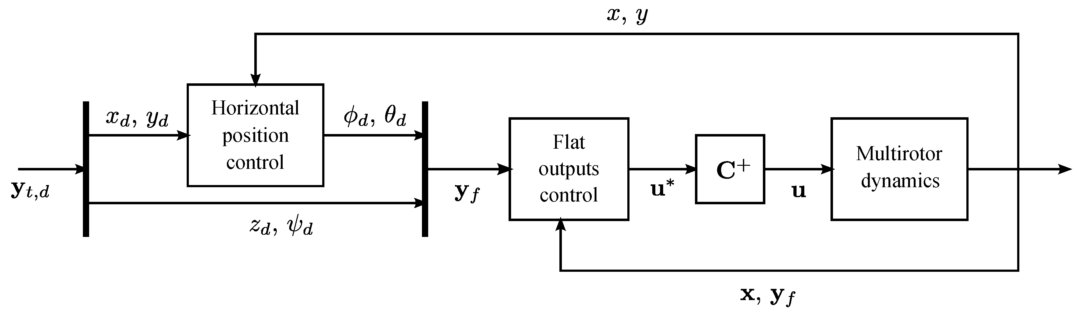
4.2. Control of the Quadrotor

The quadrotor is an under-actuated system and, thus, requires a nested-loop control structure, as shown in Figure 5. NDI provides a linear mapping between the new pseudo-input vector $\widehat{\mathbf{u}}={[{\widehat{u}}_z,{\widehat{u}}_{\varphi },{\widehat{u}}_{\theta },{\widehat{u}}_{\psi }]}^T$ and a flat output vector ${\mathbf{y}}_f={[z,\varphi ,\theta ,\psi ]}^T$ [4]. This linearised system is then stabilised using state feedback control. Thus, the inverted dynamics of the flat outputs and corresponding state feedbacks comprise the flat output controller. However, it is desirable to define a second vector of tracking outputs ${\mathbf{y}}_t={[x,y,z,\psi ]}^T$ for which a trajectory may be specified. Thus, it is necessary to obtain roll and pitch commands from a horizontal position controller, which may then be supplied to the flat output controller.

Figure 5. Structure of under-actuated multirotor controller.

Figure 5. Structure of under-actuated multirotor controller.

First, the flat output controller is specified. Noting the dynamics of the system in Equation (15) and the general linearising feedback expression in Equation (23), the component terms are thus:

$$\begin{array}{ccccc}\hfill a\left(\mathbf{x}\right)& =\left[\begin{array}{c}-\frac{mg}{cos\varphi cos\theta }\\ {\mathbf{0}}_{3,1}\end{array}\right]\hfill & \hfill \hspace{1em}\hspace{1em}\hspace{1em}& \hfill b\left(\mathbf{x}\right)& =\left[\begin{array}{cc}\frac{mg}{cos\varphi cos\theta }& {\mathbf{0}}_{1,3}\\ {\mathbf{0}}_{3,1}& \mathbf{I}\end{array}\right]\hfill \end{array}$$

(30)

Thus, the mapping between flat output ${\mathbf{y}}_f$ and new pseudo-input $\widehat{\mathbf{u}}$ is linearised, with the resulting feedbacks:

$$\begin{array}{ccccc}\hfill u_z& =\frac{m({\widehat{u}}_z-g)}{cos\varphi cos\theta }\hfill & \hfill \hspace{1em}\hspace{1em}\hspace{1em}& \hfill \left[\begin{array}{c}{u}_{\varphi }\\ u_{\theta }\\ u_{\psi }\end{array}\right]& =\mathbf{I}\left[\begin{array}{c}{\widehat{u}}_{\varphi }\\ {\widehat{u}}_{\theta }\\ {\widehat{u}}_{\psi }\end{array}\right]\hfill \end{array}$$

(31)

where the new pseudo-inputs are specified by the feedback control laws:

$$\begin{array}{cccc}\hfill {\widehat{u}}_z& =K_{p1}(z_d-z)+K_{p2}({\dot{z}}_d-\dot{z})\hfill & \hfill \hspace{1em}\hspace{1em}& \hfill \left[\begin{array}{c}{\widehat{u}}_{\varphi }\\ {\widehat{u}}_{\theta }\\ {\widehat{u}}_{\psi }\end{array}\right]={\mathbf{K}}_{a1}\left({\eta }_d-\eta \right)+{\mathbf{K}}_{a2}\left({\dot{\eta }}_d-\dot{\eta }\right)\end{array}$$

(32)

Next, the horizontal position controller is designed. This also comprises a non-linear feedback and a state feedback controller, which then produce the roll and pitch commands for a given trajectory in x and y. Considering again the quadrotor dynamics described by Equation (15), if the output is considered ${[x,y]}^T$ and the input ${[sin\varphi ,sin\theta ]}^T$, then the components of the general feedback expression are:

$$\begin{array}{ccccc}\hfill a\left(\mathbf{x}\right)& =\left[\begin{array}{c}0\\ 0\end{array}\right]\hfill & \hfill \hspace{1em}\hspace{1em}\hspace{1em}& \hfill b\left(\mathbf{x}\right)& =\left[\begin{array}{cc}\frac{msin\psi }{u_z}& -\frac{mcos\psi }{u_z}\\ \frac{mcos\psi }{u_{z}cos\varphi }& \frac{msin\psi }{u_{z}cos\varphi }\end{array}\right]\hfill \end{array}$$

(33)

Thus, the roll and pitch commands to the flat output controller are obtained from the horizontal position controller, using the non-linear feedback:

$$\begin{array}{cc}\hfill {\varphi }_d& =-arcsin\left(\frac{m({\widehat{u}}_{x}sin\psi -{\widehat{u}}_{y}cos\psi )}{u_z}\right)\hfill \\ \hfill {\theta }_d& =-arcsin\left(\frac{m({\widehat{u}}_{x}cos\psi +{\widehat{u}}_{y}sin\psi )}{u_{z}cos\varphi }\right)\hfill \end{array}$$

(34)

where the new inputs ${\widehat{u}}_x$ and ${\widehat{u}}_y$ control motion in the horizontal plane and are specified by the state feedback laws:

$$\begin{array}{cc}\hfill \left[\begin{array}{c}{\widehat{u}}_x\\ {\widehat{u}}_y\end{array}\right]& =K_{p1}\left[\begin{array}{c}{x}_d-x\\ y_d-y\end{array}\right]+K_{p2}\left[\begin{array}{c}{\dot{x}}_d-\dot{x}\\ {\dot{y}}_d-\dot{y}\end{array}\right]\hfill \end{array}$$

(35)

The gains of the roll and pitch controllers are specified, such that the closed-loop response of ϕ and θ to set-points ${\varphi }_d$ and ${\theta }_d$ is relatively fast in comparison to the horizontal position response. The closed-loop horizontal position response is then assumed to be linear when the roll and pitch response is sufficiently fast, or:

$$\begin{array}{c}\hfill \left[\begin{array}{c}\ddot{x}\\ \ddot{y}\end{array}\right]\approx \left[\begin{array}{c}{\widehat{u}}_x\\ {\widehat{u}}_y\end{array}\right]\text{when}\frac{\Phi \left(s\right)}{{\Phi }_d\left(s\right)}=\frac{\Theta \left(s\right)}{{\Theta }_d\left(s\right)}\approx 1\end{array}$$

(36)

Finally, the pseudo-inputs ${\mathbf{u}}^{*}$ are reconfigured into the individual rotor inputs by inverting the control matrix described by Equation (14) using the method in Equation (11).

4.3. Control of the Hexarotor

As the hexarotor is fully-actuated, it may be controlled by a single feedback loop, as shown in Figure 6. NDI then provides a linear mapping between the new pseudo-input vector $\widehat{\mathbf{u}}={[{\widehat{u}}_x,{\widehat{u}}_y,{\widehat{u}}_z,{\widehat{u}}_{\varphi },{\widehat{u}}_{\theta },{\widehat{u}}_{\psi }]}^T$ and the flat output vector ${\mathbf{y}}_f={[x,y,z,\varphi ,\theta ,\psi ]}^T$. As with the quadrotor, the linearised system is then stabilised using state feedback control. Additionally, it is theoretically possible to specify trajectories for all six degrees of freedom; thus, the tracking outputs are defined ${\mathbf{y}}_t={\mathbf{y}}_f$.

Figure 6. Structure of the fully-actuated multirotor controller.

Figure 6. Structure of the fully-actuated multirotor controller.

Noting the hexarotor’s dynamic model in Equation (18), the components of the general feedback described by Equation (23) are:

$$\begin{array}{ccccc}\hfill a\left(\mathbf{x}\right)& =\left[\begin{array}{c}-mg{\mathbf{R}}_{\mathcal{W}}^{\mathcal{B}}\widehat{\mathbf{z}}\\ {\mathbf{0}}_{3,1}\end{array}\right]\hfill & \hfill \hspace{1em}\hspace{1em}\hspace{1em}& \hfill b\left(\mathbf{x}\right)& =\left[\begin{array}{cc}m{\mathbf{R}}_{\mathcal{W}}^{\mathcal{B}}& {\mathbf{0}}_{3,3}\\ {\mathbf{0}}_{3,3}& \mathbf{I}\end{array}\right]\hfill \end{array}$$

(37)

Thus, the mapping between flat output ${\mathbf{y}}_f$ and new pseudo-input $\mathbf{u}$ is linearised, with the resulting feedbacks:

$$\begin{array}{ccccc}\hfill \left[\begin{array}{c}{u}_x\\ u_y\\ u_z\end{array}\right]& =m{\mathbf{R}}_{\mathcal{W}}^{\mathcal{B}}\left({\ddot{\mathbf{r}}}_d-g\widehat{\mathbf{z}}\right)\hfill & \hfill \hspace{1em}\hspace{1em}\hspace{1em}& \hfill \left[\begin{array}{c}{u}_{\varphi }\\ u_{\theta }\\ u_{\psi }\end{array}\right]& =\mathbf{I}{\ddot{\eta }}_d\hfill \end{array}$$

(38)

where the new pseudo-inputs are specified by the feedback control laws:

$$\begin{array}{ccccc}\hfill \left[\begin{array}{c}{\widehat{u}}_x\\ {\widehat{u}}_y\\ {\widehat{u}}_z\end{array}\right]& =K_{p1}({\mathbf{r}}_d-\mathbf{r})+K_{p2}({\dot{\mathbf{r}}}_d-\dot{\mathbf{r}})\hfill & \hfill \hspace{1em}\hspace{1em}\hspace{1em}& \hfill \left[\begin{array}{c}{\widehat{u}}_{\varphi }\\ {\widehat{u}}_{\theta }\\ {\widehat{u}}_{\psi }\end{array}\right]& ={\mathbf{K}}_{a1}\left({\eta }_d-\eta \right)+{\mathbf{K}}_{a2}\left({\dot{\eta }}_d-\dot{\eta }\right)\hfill \end{array}$$

(39)

The pseudo-inputs ${\mathbf{u}}^{*}$ are then reconfigured into the individual rotor inputs by employing the control allocation method of Equation (11) on the hexarotor’s control matrix, described in Equation (17).

While the hexarotor is theoretically fully-actuated and, thus, does not require a separate horizontal position controller, in practice, this is not the case. In reality, actuator limits on the aircraft’s rotors limit the maximum thrust and torque that can be generated. As the angle of inclination α of the hexarotor’s individual thrust vectors must be small to maintain sufficient lift force for hover, the component of thrust that can be generated in the horizontal plane is relatively small. Therefore, in practice, while the vehicle can translate in the horizontal plane without impact on the other degrees of freedom, this translation is subject to an upper limit on acceleration.

To ensure that fast lateral motion of the hexarotor is still achievable, the hexarotor is designed to roll or pitch when the horizontal acceleration limit is exceeded. As with the quadrotor, roll and pitch trajectories are therefore not specified directly, but are dependent on the trajectories in x and y. The relationship used to define roll and pitch commands is then similar to that of the quadrotor, but instead acts on the difference between commanded acceleration, ${\widehat{u}}_x={\ddot{x}}_d$ or ${\widehat{u}}_y={\ddot{y}}_d$, and the acceleration limit $a_{max}$. For translation in x, this difference $\Delta {\widehat{u}}_x$ is defined by the logic:

$$\Delta {\widehat{u}}_x=\left\{\begin{array}{cc}{\widehat{u}}_x+a_{max}\hfill & \text{if}{\widehat{u}}_x\le -a_{max}\hfill \\ 0\hfill & \text{if}-a_{max}\le {\widehat{u}}_x\le a_{max}\hfill \\ {\widehat{u}}_x-a_{max}\hfill & \text{if}{\widehat{u}}_x\ge a_{max}\hfill \end{array}\right.$$

(40)

while $\Delta {\widehat{u}}_y$ is defined similarly. The resulting roll and pitch commands are then found from:

$$\begin{array}{cc}\hfill {\varphi }_d& =-arcsin\left(\frac{m(\Delta {\widehat{u}}_{x}sin\psi -\Delta {\widehat{u}}_{y}cos\psi )}{u_z}\right)\hfill \\ \hfill {\theta }_d& =-arcsin\left(\frac{m(\Delta {\widehat{u}}_{x}cos\psi +\Delta {\widehat{u}}_{y}sin\psi )}{u_{z}cos\varphi }\right)\hfill \end{array}$$

(41)

Thus, if the lateral acceleration is within the specified limits, the vehicle remains level. If the acceleration is greater than the specified limit, the hexarotor tilts to increase the horizontal acceleration component and to maintain tracking accuracy. While the ability to directly specify roll and pitch trajectories is sacrificed in this instance, further augmentation of the controller could permit decoupled roll and pitch control under low lateral acceleration.

4.4. Control of the Octorotor

As with the quadrotor, the octorotor is under-actuated and requires a nested feedback loop structure to control all six degrees of freedom. NDI provides again a linear mapping between the new pseudo-input vector $\widehat{\mathbf{u}}={[{\widehat{u}}_z,{\widehat{u}}_{\varphi },{\widehat{u}}_{\theta },{\widehat{u}}_{\psi }]}^T$ and the flat output vector ${\mathbf{y}}_f={[z,\varphi ,\theta ,\psi ]}^T$. As the pseudo-inputs and outputs of the quadrotor and octorotor are identical, the rigid body models of each are also identical. Thus, the linearising feedback for the octorotor’s flat outputs are also expressed by Equation (31) and the resulting flat output controller by Equation (32). The roll and pitch commands and resulting horizontal position controller are similarly described by Equations (34) and (35), respectively.

Having obtained the pseudo-inputs for a given four-dimensional trajectory, it is necessary to obtain the individual rotor inputs for the octorotor. Consider the control matrix $\mathbf{C}$ described in Equation (21). As $\mathbf{C}$ is not square in this instance, the inverse ${\mathbf{C}}^{-1}$ does not exist. Here, the use of the pseudo-inverse ${\mathbf{C}}^{+}$ is justified. Thus, the control allocation is again accomplished using Equation (11).

5. Operational Differences Between Configurations

It is clear from the description of the three configurations that the closed-loop performance of the hexarotor will differ from the other two platforms. This is due to the independence of the horizontal position outputs from roll and pitch at low accelerations. However, each platform also demonstrates differences in operation. In comparing the operational performance of each multirotor configuration, some assumptions are made. First, it is assumed that each system employs the same components. Rotors of identical mass and performance are used in each case. The thrust gain $K_T$ and torque gain $K_Q$ described by the rotor model in Equation (4) are thus identical for each system. Next, it is assumed that the airframe of each platform consists of a series of bars of a square cross-section and identical mass per unit length. Finally, the avionics of each aircraft is assumed to be identical for each vehicle and located at its centre of mass. Using these assumptions, the mass and moments of inertia of each configuration were determined and are shown in Table 1. It is clear then that the octorotor has greater mass and moments of inertia than the hexarotor and octorotor, while the hexarotor may be considered similarly with respect to the quadrotor.

The final assumption is that an actuator limit exists that places a minimum and maximum on the thrust and torque output of each rotor. A given rotor input u is then subject to the constraint:

$$u=\left\{\begin{array}{cc}{u}_{\text{min}}\hfill & \text{if}u\le u_{\text{min}}\hfill \\ u\hfill & \text{if}{u}_{\text{min}}<0<u_{\text{max}}\hfill \\ u_{\text{max}}\hfill & \text{if}u\ge u_{\text{max}}\hfill \end{array}\right.$$

(42)

where $u_{\text{min}}$ is the input corresponding to zero throttle and $u_{\text{max}}$ is the input corresponding to maximum throttle. The values for these limits employed in the simulation are given in Table 1. The use of dynamic inversion and the resulting consistency in closed-loop performance across each configuration assumes that each system is described by a continuous-time model, such as those described in Equations (15), (18) and (22). The inclusion of actuator limits represents a discontinuity in each system, which is not considered by the dynamic inversion process. Thus, given the differing masses and inertias of each vehicle, the possibility of different closed-loop performance arises when these actuator limits are reached.

Table 1. Multirotor properties for simulation testing.

Property	Symbol	Value	Unit
Quadrotor mass	$m_Q$	$0.5$	kg
Hexarotor mass	$m_H$	$0.7$	kg
Octorotor mass	$m_O$	$1.0$	kg
Quadrotor inertia about $x^{\mathcal{B}}$	$I_{x,Q}$	$0.0054$	kg m2
Quadrotor inertia about $y^{\mathcal{B}}$	$I_{y,Q}$	$0.0054$	kg m2
Quadrotor inertia about $z^{\mathcal{B}}$	$I_{z,Q}$	$0.0107$	kg m2
Hexarotor inertia about $x^{\mathcal{B}}$	$I_{x,H}$	$0.0085$	kg m2
Hexarotor inertia about $y^{\mathcal{B}}$	$I_{y,H}$	$0.0085$	kg m2
Hexarotor inertia about $z^{\mathcal{B}}$	$I_{z,H}$	$0.0149$	kg m2
Octorotor inertia about $x^{\mathcal{B}}$	$I_{x,O}$	$0.0167$	kg m2
Octorotor inertia about $y^{\mathcal{B}}$	$I_{y,O}$	$0.0734$	kg m2
Octorotor inertia about $z^{\mathcal{B}}$	$I_{z,O}$	$0.0901$	kg m2
Quadrotor/hexarotor rotor arm	l	$0.2$	m
Octorotor near rotor arm in x	$l_{x1}$	$\sqrt{0.02}$	m
Octorotor far rotor arm in x	$l_{x2}$	$\sqrt{0.02}+0.3$	m
Octorotor rotor arm in y	$l_y$	$\sqrt{0.02}$	m
Hexarotor rotor inclination	α	15	°
Thrust gain	$K_T$	60	N
Torque gain	$K_Q$	1	N m
Lower input limit	$u_{\text{min}}$	0	–
Upper input limit	$u_{\text{max}}$	$0.05$	–
Hexarotor max lateral acceleration	$a_{\text{max}}$	$1.2$	m s−2

Table 1. Multirotor properties for simulation testing.

Property	Symbol	Value	Unit
Quadrotor mass	$m_Q$	$0.5$	kg
Hexarotor mass	$m_H$	$0.7$	kg
Octorotor mass	$m_O$	$1.0$	kg
Quadrotor inertia about $x^{\mathcal{B}}$	$I_{x,Q}$	$0.0054$	kg m2
Quadrotor inertia about $y^{\mathcal{B}}$	$I_{y,Q}$	$0.0054$	kg m2
Quadrotor inertia about $z^{\mathcal{B}}$	$I_{z,Q}$	$0.0107$	kg m2
Hexarotor inertia about $x^{\mathcal{B}}$	$I_{x,H}$	$0.0085$	kg m2
Hexarotor inertia about $y^{\mathcal{B}}$	$I_{y,H}$	$0.0085$	kg m2
Hexarotor inertia about $z^{\mathcal{B}}$	$I_{z,H}$	$0.0149$	kg m2
Octorotor inertia about $x^{\mathcal{B}}$	$I_{x,O}$	$0.0167$	kg m2
Octorotor inertia about $y^{\mathcal{B}}$	$I_{y,O}$	$0.0734$	kg m2
Octorotor inertia about $z^{\mathcal{B}}$	$I_{z,O}$	$0.0901$	kg m2
Quadrotor/hexarotor rotor arm	l	$0.2$	m
Octorotor near rotor arm in x	$l_{x1}$	$\sqrt{0.02}$	m
Octorotor far rotor arm in x	$l_{x2}$	$\sqrt{0.02}+0.3$	m
Octorotor rotor arm in y	$l_y$	$\sqrt{0.02}$	m
Hexarotor rotor inclination	α	15	°
Thrust gain	$K_T$	60	N
Torque gain	$K_Q$	1	N m
Lower input limit	$u_{\text{min}}$	0	–
Upper input limit	$u_{\text{max}}$	$0.05$	–
Hexarotor max lateral acceleration	$a_{\text{max}}$	$1.2$	m s−2

The operational performance of each configuration is compared in a simulation, using the properties described in Table 1. Identical controller gains are employed for each system, yielding comparative closed-loop performance. Each system is instructed to track a four-dimensional trajectory in the tracking output ${\mathbf{y}}_t={[x,y,z,\psi ]}^T$, which is defined by a series of fifth-order polynomials. Several cases are considered, which adjust this trajectory to highlight the differences in the closed-loop performance of each platform. Specifically, these differences are the increased number of actuators of the hexarotor and the impact of actuator limits on trajectory tracking.

5.1. Controller Gains and Trajectory Definition

Using non-linear dynamic inversion and with the assumption of a continuous closed-loop response, each multirotor configuration can be described in closed-loop by the relationships in Equation (29). As the use of a linearising feedback eliminates differences in platform-specific properties, identical controller gains may be used for all configurations. For the investigations described here, these gains are selected to be:

$$\begin{array}{ccccc}\hfill K_{p1}& =15.21\hfill & \hfill \hspace{1em}\hspace{1em}\hspace{1em}& \hfill K_{p2}& =7.8\hfill \\ \hfill {\mathbf{K}}_{a1}& =\left[\begin{array}{ccc}1521& 0& 0\\ 0& 1521& 0\\ 0& 0& 15.21\end{array}\right]\hfill & \hfill \hspace{1em}\hspace{1em}\hspace{1em}& \hfill {\mathbf{K}}_{a2}& =\left[\begin{array}{ccc}78& 0& 0\\ 0& 78& 0\\ 0& 0& 7.8\end{array}\right]\hfill \end{array}$$

which result in a critically-damped response in both position and attitude. The gains are sufficiently high that the possibility of reaching discontinuous actuator or acceleration limits exists, depending on the trajectory commands to the controller.

Each system’s tracking output trajectory ${\mathbf{y}}_t\left(t\right)$ is specified using the polynomial approach described by [20]. Each multirotor is commanded to track displacement and velocity trajectories defined by the general polynomials:

$$\begin{array}{cc}\hfill y_{d,i}\left(t\right)& =a_{0,i}+a_{1,i}t+\frac{1}{2}{a}_{2,i}{t}^2+\frac{1}{6}{a}_{3,i}{t}^3+\frac{1}{12}{a}_{4,i}{t}^4+\frac{1}{20}{a}_{5,i}{t}^5\hfill \\ \hfill {\dot{y}}_{d,i}\left(t\right)& =a_{1,i}+a_{2,i}t+\frac{1}{2}{a}_{3,i}{t}^2+\frac{1}{3}{a}_{4,i}{t}^3+\frac{1}{4}{a}_{5,i}{t}^4\hfill \end{array}$$

(43)

where $y_{d,i}$ is an element of the desired output vector ${\mathbf{y}}_d={[x_d,y_d,z_d,{\psi }_d]}^T$ and ${\dot{y}}_{d,i}$ is an element of its derivative ${\dot{\mathbf{y}}}_d={[{\dot{x}}_d,{\dot{y}}_d,{\dot{z}}_d,{\dot{\psi }}_d]}^T$. The trajectories may alternatively be formulated as the matrix relationships:

$$\begin{array}{ccccc}\hfill {\mathbf{y}}_d\left(t\right)& =\mathbf{A}\left[\begin{array}{c}1\\ t\\ \frac{1}{2}{t}^2\\ \frac{1}{6}{t}^3\\ \frac{1}{12}{t}^4\\ \frac{1}{20}{t}^5\end{array}\right]\hfill & \hfill \hspace{1em}\hspace{1em}\hspace{1em}& \hfill {\dot{\mathbf{y}}}_d\left(t\right)& =\mathbf{A}\left[\begin{array}{c}0\\ 1\\ t\\ \frac{1}{2}{t}^2\\ \frac{1}{3}{t}^3\\ \frac{1}{4}{t}^4\end{array}\right]\hfill \end{array}$$

(44)

where $\mathbf{A}$ is the $4\times 6$ matrix describing the coefficients $a_{0,i}\dots a_{5,i}$ for each element i in ${\mathbf{y}}_d$ and ${\dot{\mathbf{y}}}_d$. These coefficients are chosen, such that they prescribe a smooth trajectory between an initial displacement ${\mathbf{y}}_{d,0}$ and velocity ${\dot{\mathbf{y}}}_{d,0}$ and final displacement ${\mathbf{y}}_{d,f}$ and velocity ${\dot{\mathbf{y}}}_{d,f}$. For brevity, these displacements and velocities are not given here; however, the resulting matrix of coefficients $\mathbf{A}$ is. The desired roll and pitch trajectories are specified by the horizontal position controller of each vehicle or, for the hexarotor in low-acceleration flight, fixed at zero.

Having defined the general state feedback controller for each linearised system and the general form of the desired trajectories, each system is commanded to follow an identical four-dimensional trajectory ${\mathbf{y}}_d\left(t\right)$, which tests different aspects of the operational performance of each vehicle.

5.2. Control Effort During Accurate Trajectory Tracking

The multirotors are commanded to follow a four-dimensional trajectory as defined by Equation (44), with the matrix of coefficients:

$$\mathbf{A}=\left[\begin{array}{cccccc}\left[r\right]0& 0& 0& 1.4400& -0.8640& 0.1152\\ 0& 0& 0& 0& 0.0480& -0.0096\\ 0& 0& 0& -0.6720& 0.4224& -0.0576\\ 0& 0& 0& 0.4800& -0.2880& 0.0384\end{array}\right]$$

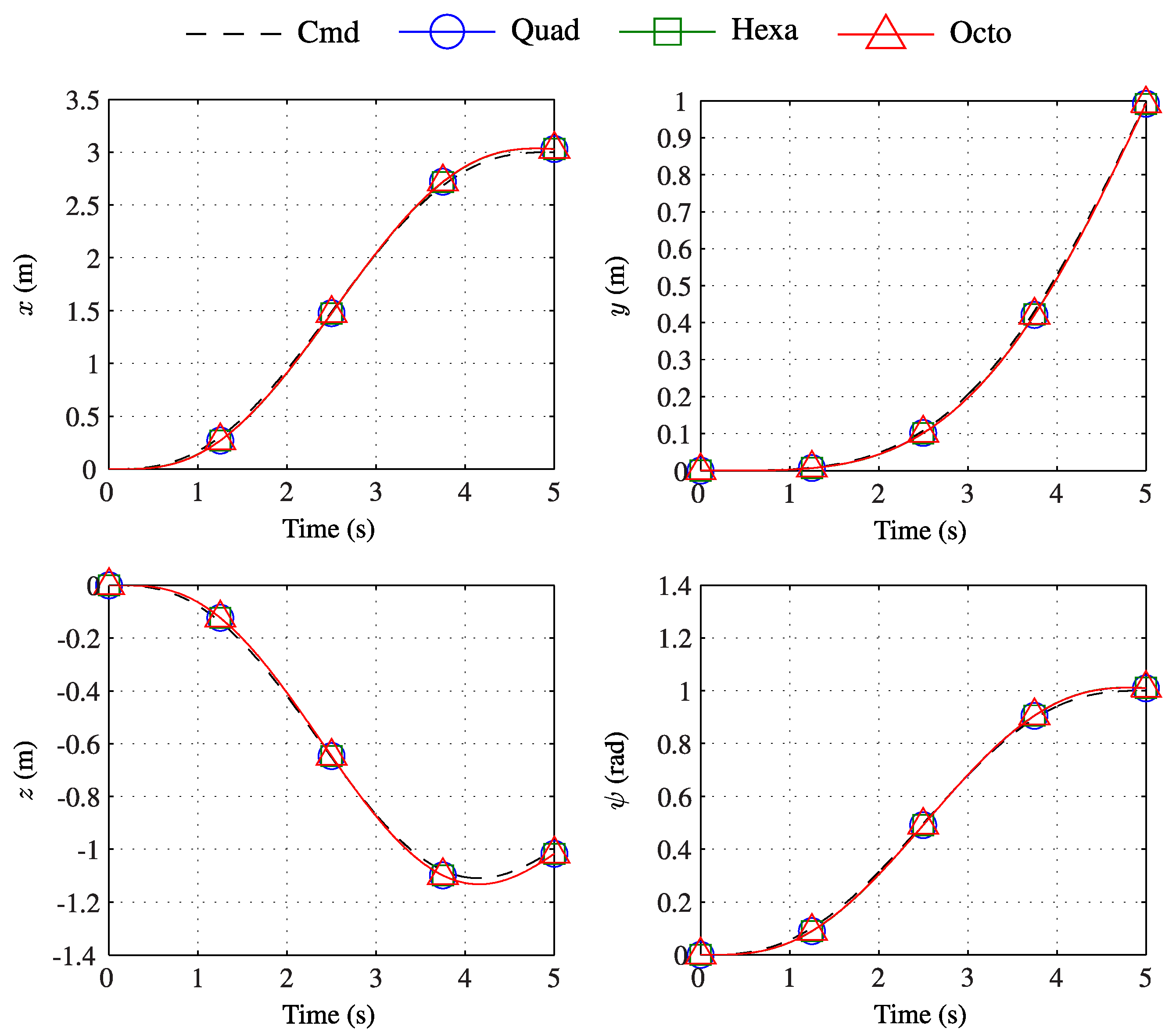
This produces a trajectory that is tracked with negligible error by each configuration, using the controller gains previously specified. The resulting response of each tracking output is shown against the corresponding reference trajectory in Figure 7. By design, the response of each configuration in these outputs is identical and follows the reference trajectory closely.

Figure 7. Dynamic response in position and heading for each multirotor when accurately tracking a commanded path.

Figure 7. Dynamic response in position and heading for each multirotor when accurately tracking a commanded path.

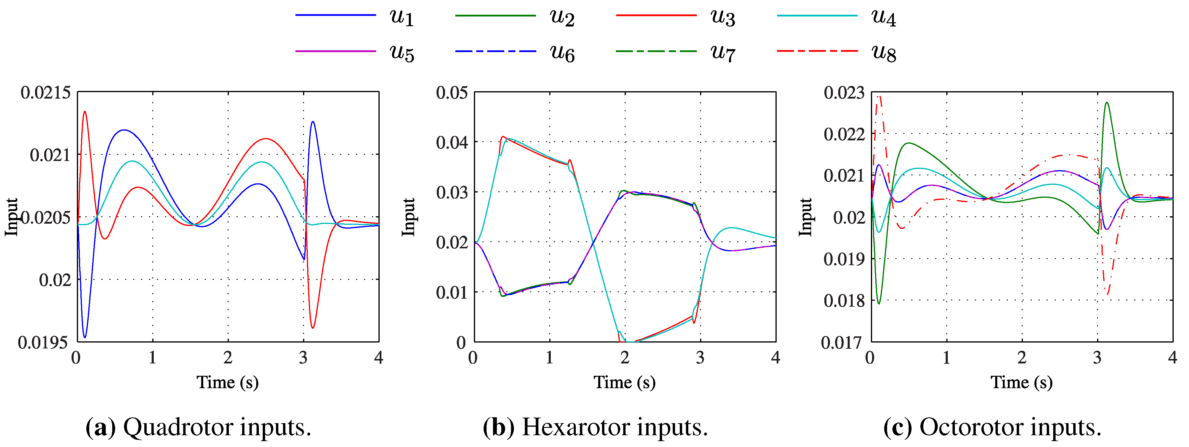
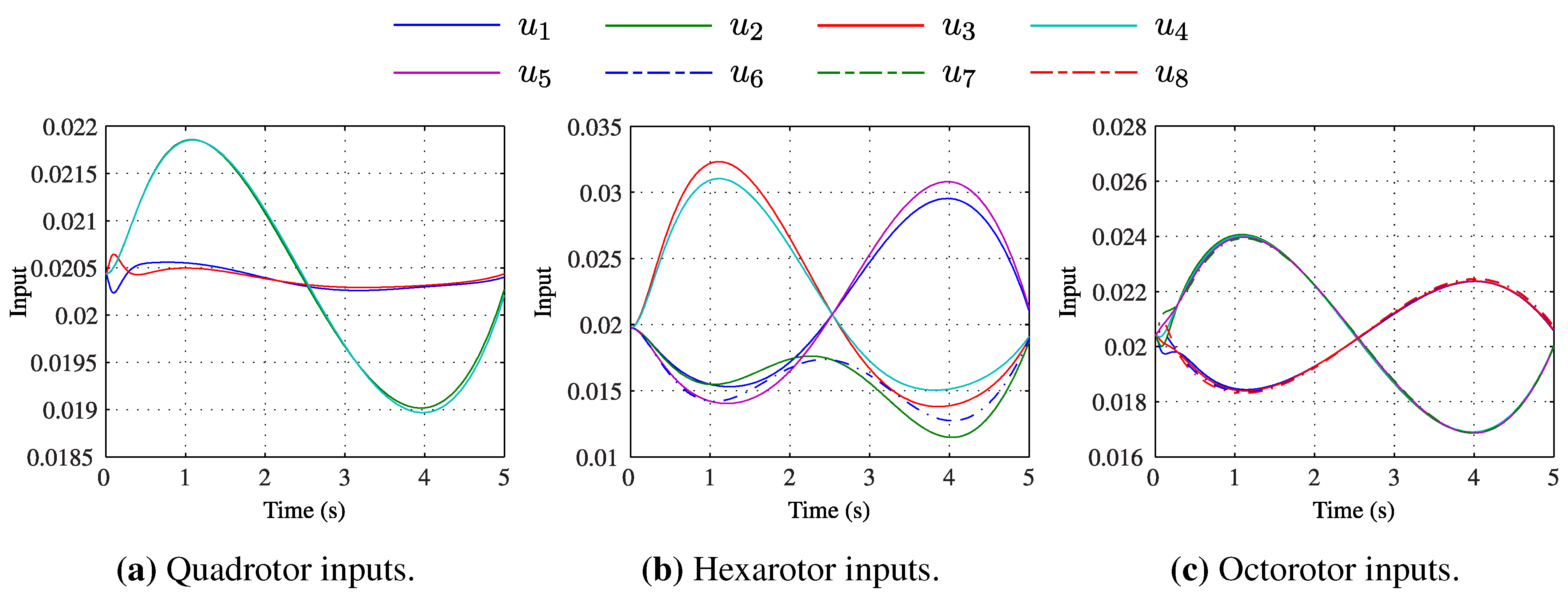
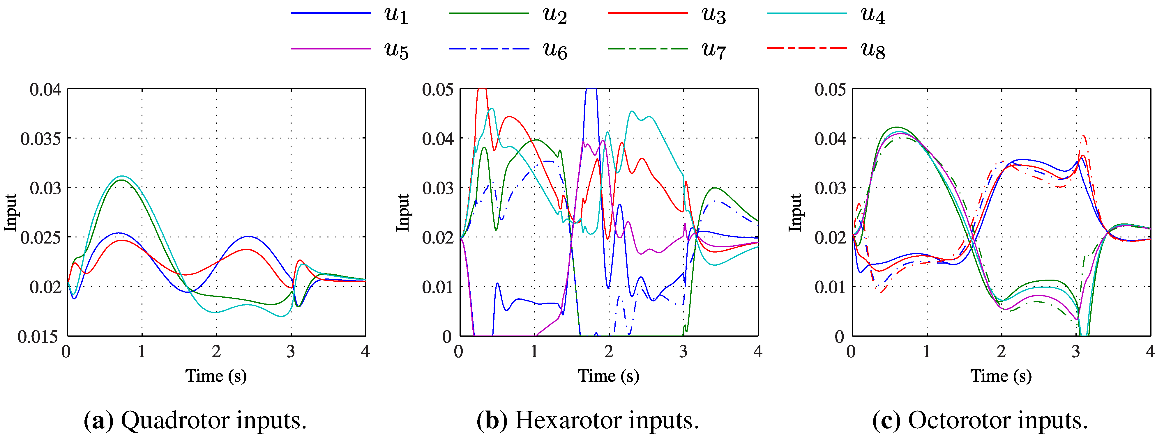
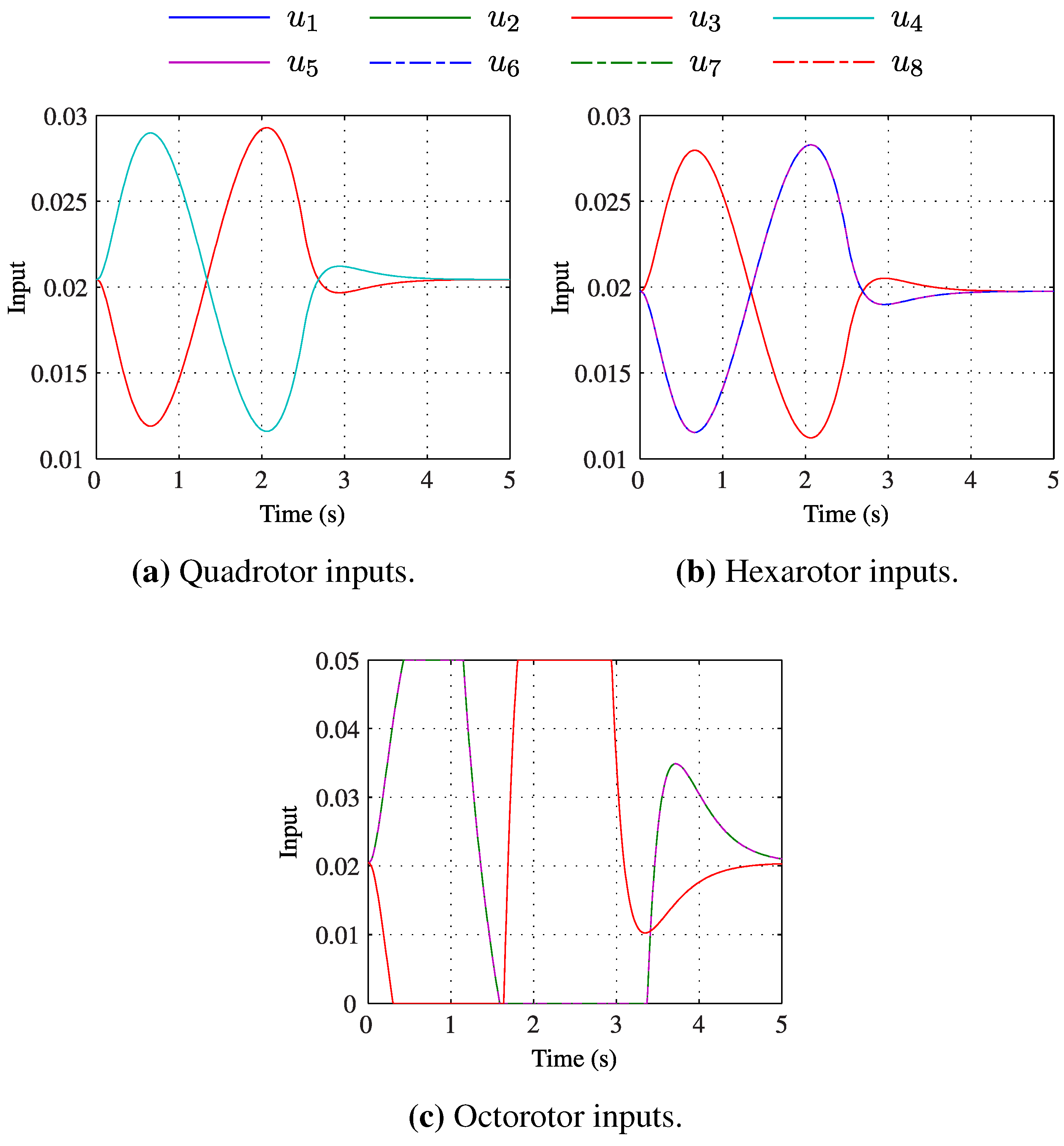
While the output histories of each vehicle are identical, the geometries and behaviours are not. As a result, it is expected that the input histories of each configuration will be different. Of primary interest is the control effort required by each system, both instantaneously and over the duration of the manoeuvre. Figure 8 shows the input histories for each platform during the specified manoeuvre. As the actuator limits are not reached for any configuration, each system remains continuous and therefore linear in a closed-loop. The implication of this is that the tracking outputs will exhibit identical response, as has been demonstrated.

Figure 8. Motor input histories for each configuration while tracking a flight path with equivalent accuracy.

Figure 8. Motor input histories for each configuration while tracking a flight path with equivalent accuracy.

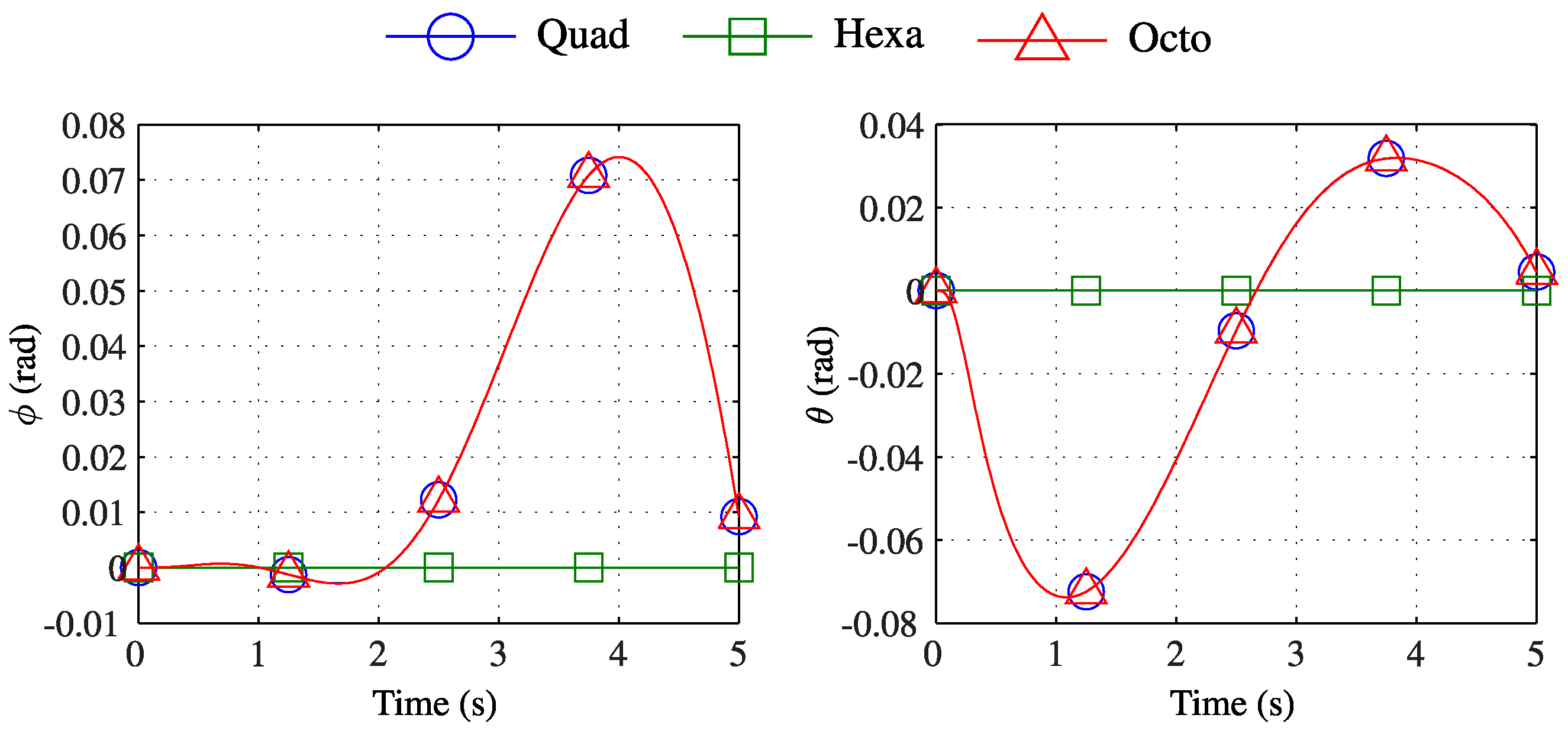
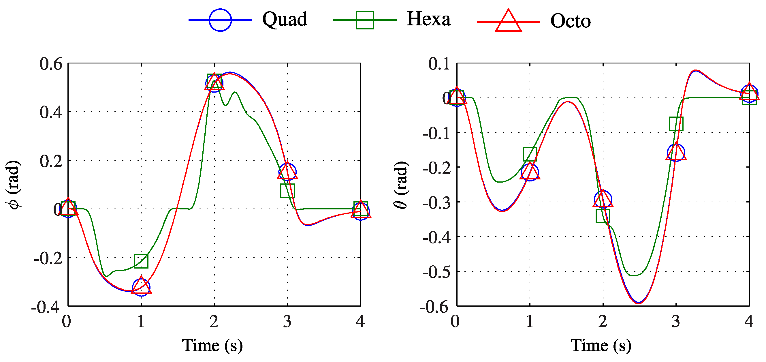
The variation in input signals for each multirotor may be discussed with reference to its configuration. The magnitude of the hexarotor inputs is shown to be greater than those of both the quadrotor and octorotor. This is due to the off-vertical rotors of the hexarotor, which allow it to translate horizontally without attitude change. Thus, while the inputs and corresponding power draw of the hexarotor are greater than the other platforms, it has the advantage of remaining level during the manoeuvre. This is demonstrated in Figure 9, where the quadrotor and octorotor, both under-actuated, show an identical roll and pitch response. In contrast, the fully-actuated hexarotor remains level during the manoeuvre.

Figure 9. Dynamic response in roll and pitch for each multirotor when accurately tracking a commanded path.

Figure 9. Dynamic response in roll and pitch for each multirotor when accurately tracking a commanded path.

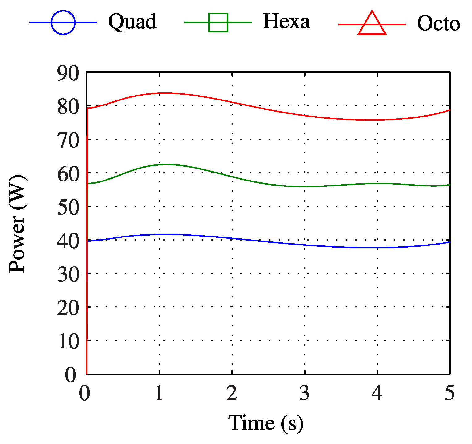
The magnitude in control signal for both the quadrotor and octorotor can be seen to be similar during the manoeuvre. However, as the octorotor has twice the number of rotors as the quadrotor, it also draws more power. This is demonstrated in Figure 10, which shows the net power of the rotors for each platform during the specified manoeuvre. Neglecting other subsystems, such as the autopilot and communications, the energy consumed by each multirotor during the manoeuvre may be compared, as shown in Table 2. Again, it is clear that the energy usage increases with the number of rotors, with an almost linear relationship.

Figure 10. Net power draw from rotors during accurate tracking of the reference trajectory.

Figure 10. Net power draw from rotors during accurate tracking of the reference trajectory.

Table 2. Energy usage for rotors only during accurate tracking of the reference trajectory.

Platform	Energy (J)
Quadrotor	197.53
Hexarotor	290.37
Octorotor	396.22

Table 2. Energy usage for rotors only during accurate tracking of the reference trajectory.

Platform	Energy (J)
Quadrotor	197.53
Hexarotor	290.37
Octorotor	396.22

5.3. Tracking Performance During Specific Manoeuvres

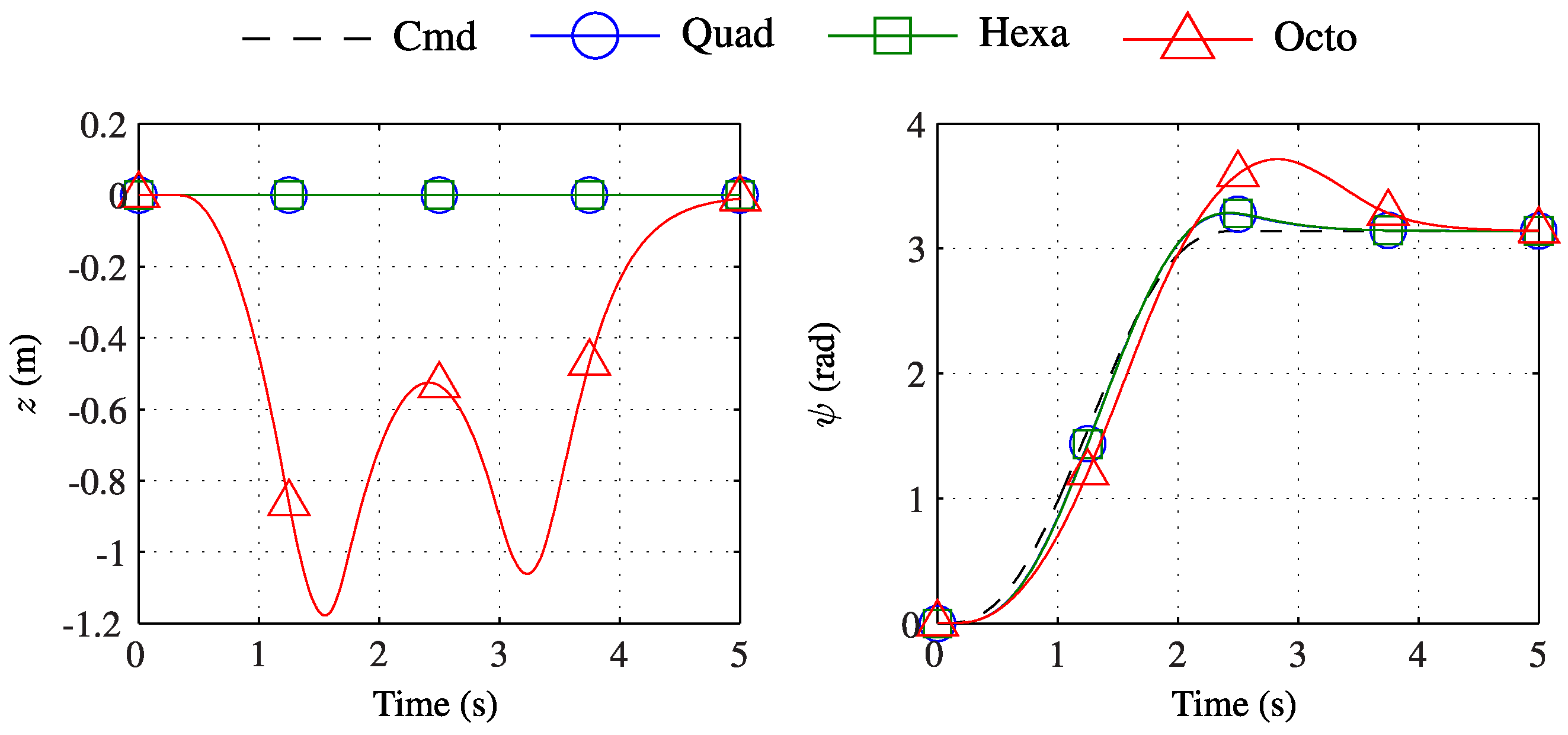
More aggressive manoeuvres may be considered. Consider any of the multirotor systems described in this paper. Use of NDI renders this continuous system near-linear in a closed-loop. The introduction of actuator limits represents a discontinuity in the system. When these limits are reached, the NDI feedback no longer eliminates the non-linearities of the now discontinuous multirotor system. As a result of the configurational differences between each multirotor, the actuator limits of each platform will be met under different conditions. It is therefore expected that the closed-loop response of each configuration will differ under conditions where actuator saturation occurs.

The operational differences of each configuration when actuator saturation occurs may be examined by defining a series of aggressive reference trajectories. These trajectories result in the actuator limits of at least one configuration being met. The resulting differences in tracking output may then be discussed with reference to each configuration’s input histories.

5.3.1. Fast Horizontal Translation

The hexarotor is capable of level, horizontal flight, as demonstrated by the previous case trajectory. However, the horizontal forces that allow this motion are limited by the actuator limits and the inclination of the rotors. An artificial limit is thus employed by the controller, as described by Equation (40). This limits level flight to a specific range of horizontal acceleration. Outside this range, the hexarotor rolls and pitches similarly to the quad- and octo-rotor. This represents another discontinuity in the system, affecting only the hexarotor in this instance.

The effects of this discontinuity are investigated by defining a fast horizontal manoeuvre, which demands an acceleration beyond the limits imposed on the hexarotor’s controller. Each multirotor is commanded to follow a trajectory in x. For brevity, only the relevant row ${\mathbf{A}}_x$ of the coefficient matrix $\mathbf{A}$ is considered. That is:

$${\mathbf{A}}_x=\left[\begin{array}{cccccc}0& 0& 0& 6.6667& -6.6667& 1.4815\end{array}\right]$$

(45)

while the remaining coefficients of $\mathbf{A}$ are zero.

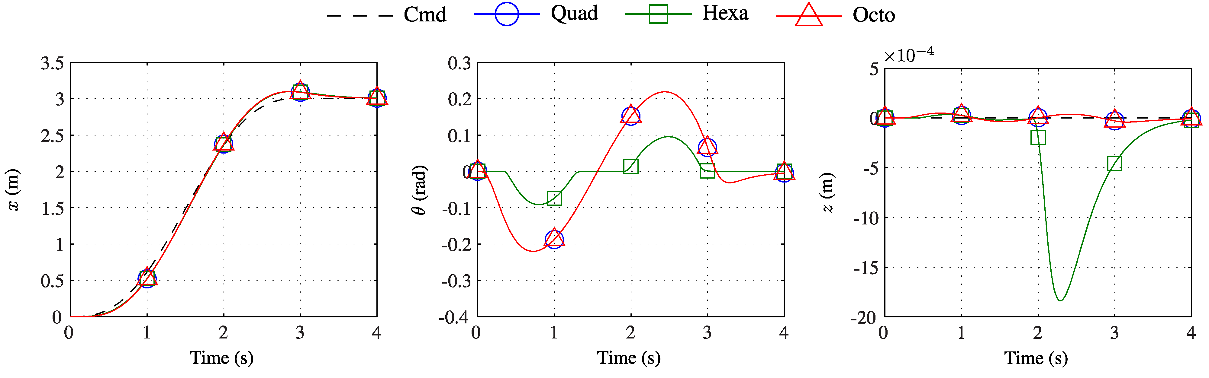
Figure 11 shows the longitudinal outputs of each configuration as it follows this trajectory. The response in the tracking output x is shown to be identical for each platform. It is expected from this result that the actuator limits of each configuration have not been met; thus, the systems remain continuous, and the linear closed-loop responses hold. The response in θ exemplifies the performance of the hexarotor when the acceleration limits are exceeded. The hexarotor remains level until its acceleration is sufficiently great for the controller to demand pitching action. The pitching response exhibits clearly discontinuous behaviour, but does not adversely affect the position response. Finally, the response in z demonstrates a negligible difference between the hexarotor and the other two configurations. It is here that actuator saturation is implied to have occurred. This is corroborated by the input histories shown in Figure 12. Actuator saturation occurs only in the hexarotor response and only briefly. The timing of the saturation coincides with the deviation in height exhibited by the hexarotor.

Figure 11. Dynamic response in longitudinal outputs for each multirotor when performing a fast horizontal translation in x.

Figure 11. Dynamic response in longitudinal outputs for each multirotor when performing a fast horizontal translation in x.

5.3.2. Fast Yaw Rotation

Yaw action in multirotors results primarily from the net torque differential of the rotors. Because of this, the yawing moment of a multirotor is typically small in comparison to the rolling or pitching moments. A large enough yaw command is therefore likely to saturate the rotors, while an equivalent roll or pitch command would not.

The occurrence of such a discontinuity in each multirotor is investigated by defining a fast yaw rotation. Each multirotor is commanded to follow a trajectory in ψ only, defined by the subset ${\mathbf{A}}_{\psi }$ of the matrix $\mathbf{A}$:

$${\mathbf{A}}_{\psi }=\left[\begin{array}{cccccc}0& 0& 0& 12.064& -14.476& 3.860\end{array}\right]$$

(46)

where the remaining elements of $\mathbf{A}$ are fixed at zero.

Figure 12. Rotor input histories for each configuration while performing a fast horizontal translation.

Figure 12. Rotor input histories for each configuration while performing a fast horizontal translation.

Figure 13 shows the height and yaw response of each multirotor while following this trajectory. It is evident from the response in ψ that the closed-loop dynamics of the octorotor are different from the other configurations. This is verified by the significant deviation in height from both the reference trajectory and the trajectories of the quad- and hexa-rotor, which are constant at $z=0$. Examination of the input histories in Figure 14 validates the assumption of a discontinuity having occurred in the octorotor dynamics. The inputs of the quad- and hexa-rotor are both within the limits for the duration of the manoeuvre. In contrast, the inputs of the octorotor are saturated for a significant duration, resulting in unpredictable behaviour.

Figure 13. Dynamic response in yaw and height outputs for each multirotor when performing a fast yaw rotation.

Figure 13. Dynamic response in yaw and height outputs for each multirotor when performing a fast yaw rotation.

As the octorotor has a greater number of rotors than either the quadrotor or hexarotor, it is capable of producing greater torque. However, with reference to Table 1, the moment of inertia about the octorotor’s z axis is significantly greater than those of the other configurations. Thus, to produce a comparable yaw response, a far greater yawing moment is required. The resulting torque demand on each rotor results in saturation of the actuators.

Figure 14. Rotor input histories for each configuration while performing a fast yaw rotation.

Figure 14. Rotor input histories for each configuration while performing a fast yaw rotation.

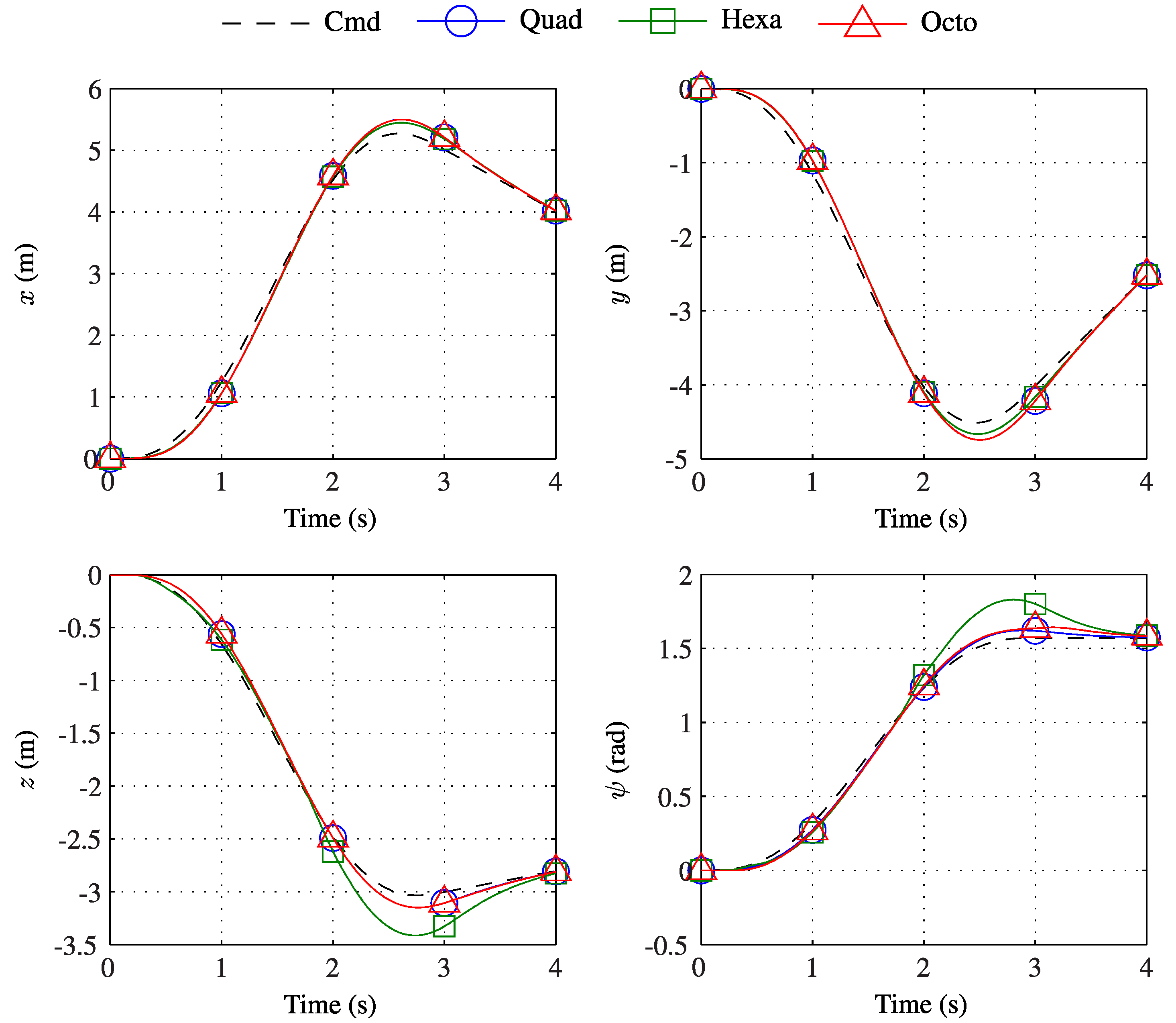
5.3.3. Fast 4D Manoeuvre

Each multirotor is commanded to perform an aggressive manoeuvre, which excites all four tracking outputs. The matrix of coefficients defining this four-dimensional trajectory is:

$$\mathbf{A}=\left[\begin{array}{cccccc}0& 0& 0& 13.778& -14.222& 3.210\\ 0& 0& 0& -12.889& 13.556& -3.086\\ 0& 0& 0& -7.200& 7.289& -1.630\\ 0& 0& 0& 3.491& -3.491& 0.776\end{array}\right]$$

(47)

Figure 15 shows the response of each tracking output in following this trajectory. Two results are clear. First, no multirotor tracks the trajectory with perfect accuracy, although the error is minimal in most cases. Consideration of the input histories in Figure 16 indicates that this is not due to actuator saturation. Instead, the tracking error is due to the speed of the closed-loop response of each multirotor system and that of the time-variant reference trajectory.

Second, while the quad- and octo-rotor have comparable tracking output responses, the hexarotor does not. Examination of Figure 16 highlights that this is due to actuator saturation, which occurs in several instances during the hexarotor flight. Figure 17 demonstrates that the hexarotor does not remain level for the duration of the flight. The hexarotor’s horizontal position controller can act to reduce the possibility of actuator saturation by rolling or pitching during large horizontal accelerations. However, it does not compensate for high acceleration in several dimensions. The combination of horizontal, vertical and yawing motion is enough to cause actuator saturation.

Figure 15. Dynamic response in position and heading for each multirotor when tracking a fast four-dimensional path.

Figure 15. Dynamic response in position and heading for each multirotor when tracking a fast four-dimensional path.

Figure 16. Motor input histories for each configuration while tracking a fast four-dimensional path.

Figure 16. Motor input histories for each configuration while tracking a fast four-dimensional path.

Figure 17. Dynamic response in roll and pitch for each multirotor when accurately tracking a commanded path.

Figure 17. Dynamic response in roll and pitch for each multirotor when accurately tracking a commanded path.

6. Discussion and Conclusions

This paper has demonstrated the differences in the configuration, control and operational performance of three specific multirotor platforms. The investigations described here are of deliberately limited scope, considering a single control strategy and employing specific assumptions about the design of each multirotor. Nevertheless, some discussion may be made and some conclusions drawn.

6.1. Discussion

It is clear that the use of non-linear dynamic inversion provides a useful means of obtaining a consistent closed-loop response, largely independent of configuration. This solution only holds if the multirotor is described as a continuous system. The inclusion of actuator limits represents a realistic discontinuity that uniquely affects the response of each configuration. In considering the results of the simulation testing described in this paper, it is apparent that only the quadrotor does not suffer from actuator saturation. One of the established limitations of this study is the use of identical rotor models and per-unit-length airframe masses. It is entirely feasible that other configurations may demonstrate superior performance to the quadrotor after optimisation of their designs.

The unusual design of the hexarotor affords it greater manoeuvrability over the other configurations. In reality, this is limited, as the thrust that can be generated in the horizontal plane is small in relation to thrust in the $z^{\mathcal{B}}$ axis. Again, the actuator limits imposed in these tests represent one specific case. It is entirely possible to develop a similar hexarotor platform with superior horizontal flight capabilities.

The differences between the quadrotor and octorotor are less distinct than those of the hexarotor. While the octorotor has greater mass and moments of inertia, it may also generate more thrust. The power usage described by Figure 10 implies that the octorotor draws significantly more power than the quadrotor for a simple manoeuvre. Yet, multirotors with greater than four rotors continue to be in popular use. Optimisation of the octorotor platform for mass and geometry would likely yield far greater performance than demonstrated here.

6.2. Conclusions

Neglecting more complex phenomena, each multirotor configuration may be described by identical rigid body and rotor models. The differences in each system model then arise simply from the quantity and positions of the rotors, as well as some properties, such as mass and inertia. Naturally, an increase in rotor quantity yields greater mass and inertias. This then impacts the flight performance of the aircraft. While the differing rotor arrangements present an interesting challenge in control allocation, the common aspects of the multirotor dynamics make application of NDI relatively trivial.

Non-linear dynamic inversion, popularly applied to the quadrotor in the literature, has been shown to similarly linearise and control other multirotor platforms. The benefits of NDI control include the elimination of non-linearities in a closed-loop and the ability to synthesise a consistent closed-loop response across different systems. This consistency only holds while each multirotor is described as a continuous system. The inclusion of discontinuities, such as actuator limits, introduces the necessity of operational testing to investigate the impact of these discontinuities. Here, it is clear that the configurational differences between each multirotor result in an inconsistent closed-loop response during aggressive manoeuvres.

6.3. Further Work

The flexibility of the multirotor platform lends itself to a wealth of possibilities in future investigations. Further multirotor configurations may be investigated, with variations on rotor quantity, position and orientation. Optimisation of a given configuration is also a key area of investigation. This is particularly evident in the novel, but limited hexarotor described in this paper.

Finally, the effectiveness of NDI control on the multirotor platform may be further investigated through the development of higher resolution models and experimental testing.

References

- Ireland, M.L. Investigations in Multi-Resolution Modelling of the Quadrotor Micro Air Vehicle. Ph.D. Thesis, University of Glasgow, Glasgow, UK, 2014. [Google Scholar]
- Das, A.; Subbarao, K.; Lewis, F. Dynamic inversion with zero-dynamics stabilisation for quadrotor control. IET Control Theory Appl. 2009, 3, 303–314. [Google Scholar] [CrossRef]
- Bouabdallah, S. Design and Control of Quadrotors with Application to Autonomous Flying. Ph.D. Thesis, Swiss Federal Institute of Technology, Lausanne, Switzerland, 2007. [Google Scholar]
- Mellinger, D.; Kumar, V. Minimum snap trajectory generation and control for quadrotors. In Proceedings of the International Conference on Robotics and Automation, Shanghai, China, 9–13 May 2011.
- Hall, J.; Anderson, D. Reactive route selection from pre-calculated trajectories: Application to micro-UAV path planning. Aeronaut. J. 2011, 115, 635–640. [Google Scholar]
- Ireland, M.; Anderson, D. Development of navigation algorithms for nap-of-the-earth UAV flight in a constrained urban environment. In Proceedings of the 28th International Congress of the Aeronautical Sciences, Brisbane, Australia, 23–28 September 2012.
- Anderson, D.; Carson, K. Integrated variable-fidelity modelling for remote sensing system design. In Proceedings of the SPIE Europe Defence & Security Conference, Berlin, Germany, 31 August 2009.
- Voos, H. Nonlinear control of a quadrotor micro-UAV using feedback-linearization. In Proceedings of the 2009 IEEE International Conference on Mechatronics, Malaga, Spain, 14–17 April 2009.
- Tayebi, A.; McGilvray, S. Attitude stabilization of a VTOL quadrotor aircraft. IEEE Trans. Control Syst. Technol. 2006, 14, 562–571. [Google Scholar] [CrossRef]
- Castillo, P.; Dzul, A. Real-time stabilization and tracking of a four-rotor mini rotorcraft. IEEE Trans. Control Syst. Technol. 2004, 12, 510–516. [Google Scholar] [CrossRef]
- Salazar-Cruz, S.; Lozano, R. Stabilization and nonlinear control for a novel trirotor mini-aircraft. In Proceedings of the 2005 IEEE International Conference on Robotics and Automation, Barcelona, Spain, 18–22 April 2005.
- Liu, H.; Derawi, D.; Kim, J.; Zhong, Y. Robust optimal attitude control of hexarotor robotic vehicles. Nonlinear Dyn. 2013, 74, 115–1168. [Google Scholar] [CrossRef]
- Sanca, A.; Guimarães, J.P.F.; Alsina, P.J. A real-time attitude estimation scheme for hexarotor micro aerial vehicle. In Proceedings of COBEM 2011, Natal, RN, Brazil, 24–28 October 2011.
- Toratani, D. Research and development of double tetrahedron hexa-rotorcraft (Dot-HR). In Proceedings of the 28th International Congress of the Aeronautical Sciences, Brisbane, Australia, 23–28 September 2012.
- Marks, A.; Whidborne, J.F.; Yamamoto, I. Control allocation for fault tolerant control of a VTOL octorotor. In Proceedings of the 2012 UKACC International Conference on Control IEEE, Cardiff, UK, 3–5 September 2012.
- Ryan, T.; Kim, H.J. LMI-based gain synthesis for simple robust quadrotor control. IEEE Trans. Automat. Sci. Eng. 2013, 10, 1173–1178. [Google Scholar] [CrossRef]
- Guangxun, D.; Quan, Q.; Kai-Yuan, C. Additive-state-decomposition-based dynamic inversion stabilized control of a hexacopter subject to unknown propeller damages. In Proceedings of the 32nd Chinese Control Conference, Xi’an, China, 26–28 July 2013.
- Ducard, G.J.J.; Hua, M.D. Discussion and practical aspects on control allocation for a multi-rotor helicopter. In Proceedings of the 1st International Conference on Unmanned Aerial Vehicle in Geomatics, Zurich, Switzerland, 14–16 September 2011.
- Glad, T.; Ljung, L. Control Theory: Multivariable and Nonlinear Methods; CRC Press: London, UK, 2000. [Google Scholar]
- Cowling, I. Towards Autonomy of a Quadrotor UAV. Ph.D. Thesis, Cranfield University, Cranfield, UK, 2008. [Google Scholar]
© 2015 by the authors; licensee MDPI, Basel, Switzerland. This article is an open access article distributed under the terms and conditions of the Creative Commons Attribution license (http://creativecommons.org/licenses/by/4.0/).