Article

Hotspots of Inequity in Climate Adaptation: Explaining the Stratification of U.S. Ecowelfare Using Space-Time and Machine Learning Analysis

by
Christopher Taylor Brown
* and
Yu-Ling Chang
School of Social Welfare, University of California, Berkeley, CA 94720, USA
*
Author to whom correspondence should be addressed.
Climate 2025, 13(12), 244; https://doi.org/10.3390/cli13120244 (registering DOI)
Submission received: 20 October 2025 / Revised: 26 November 2025 / Accepted: 27 November 2025 / Published: 29 November 2025

Abstract

As climate risk intensifies and ecowelfare is increasingly implicated in climate adaptation, we examine how FEMA’s Individuals and Households Program (IHP) allocates aid in the United States. We ask how and why IHP allocates aid, framing the analysis through a climate-justice lens that centers distributive and procedural equity. Using a county–year panel (2009–2022), we map funding hot/cold spots and estimate space–time models of per-recipient IHP funding, benchmarking against machine learning approaches. Results show that aid rises with a county’s own disaster frequency but falls when neighboring counties are simultaneously hit. Direct sociodemographic penalties are limited once space–time dependence is modeled, except for a persistent shortfall in counties with larger multiracial populations and a negative neighboring effect tied to Hispanic composition. Poverty and population size show positive neighboring effects, and counties in Democratic-governed states receive more aid, consistent with higher state capacity. Machine learning corroborates hazards’ primacy and highlights disaster-count thresholds and interactions. Implications for climate justice and adaptation include strengthening regional capacity, expanding language-access and navigator programs that help households apply for aid, and adopting local-national coordination standards to make ecowelfare more equitable and resilient.

1. Introduction

As climate risk intensifies, public institutions responsible for recovery and adaptation face growing strain. In the United States, the Federal Emergency Management Agency’s (FEMA) Individuals and Households Program (IHP) has emerged as a key tool in the federal government’s response to natural hazards, functioning as a form of ecowelfare or ecosocial safety net that enables climate adaptation. Yet critical aspects of IHP’s role in ameliorating climate risk remain under-examined and deeply contested. Emerging empirical work shows that IHP funds are unevenly distributed across U.S. counties, often disadvantaging populations with higher shares of residents who are poor, racially marginalized, or otherwise socially vulnerable [1,2]. These distributional patterns place IHP squarely within debates on climate justice, which ask who bears climate risks and who receives protection and recovery resources. Taken together, these findings suggest that the emerging U.S. ecowelfare state—programs that redistribute resources in response to climate risk—may reproduce and extend longstanding inequities in the legacy welfare state [3].
Building on this work, we shift attention from whether IHP is stratified to how stratification unfolds across space and time. If climate change represents not only a global ecological crisis but also a spatially and temporally uneven generator of climate risk, then we must also account for the dynamics of space and time. Yet most existing studies treat disparities in disaster aid as static or cross-sectional phenomena. They rarely examine how funding inequities persist, diffuse, or compound across adjacent jurisdictions or over the long arc of disaster compounding and government intervention [1,2,4,5,6]. One exception is Howell & Elliot [7], who did find that disasters widen racial and wealth inequalities over time. Moreover, while recent studies have begun to explore the spatial dependence of IHP stratification [1,5], space and time have yet to be jointly modeled. This article is part of a broader project on U.S. ecowelfare; a companion study examines average disparities in IHP using non-spatial panel models, whereas the present study focuses on the spatiotemporal structure and diffusion of those disparities [8].
This paper develops a space–time framework that integrates spatial econometrics and machine learning to investigate the stratification of one of the key U.S. ecowelfare programs that fosters climate adaptation. Using a county-year panel spanning 2009 to 2022, we apply a space-time kernel density estimator to identify persistent hot and cold spots in IHP expenditure per recipient. We then estimate two autoregressive spatial econometric models—a Space-Time Autoregressive (STAR) model and a Space-Time Durbin Model (STDM)—to evaluate the direct and spillover effects of sociodemographic, economic, political, and disaster-related factors. Finally, we compare these models against six predictive machine learning approaches and use a gradient-boosted decision tree (XGBoost) model to detect non-linearities and variable importance.
Throughout, we treat IHP as reactive adaptation via social protection. Although assistance is disbursed post-event, IHP redistributes climate risk and conditions households’ ability to withstand recurrent hazards. We use relief to denote immediate assistance; recovery to denote restoring pre-event functioning; and adaptation to denote adjustments that reduce climate risk or its social harms over time. Post-disaster programs like IHP can do more than one of these.
In doing so, we contribute in three ways. First, we introduce a space-time conceptualization of ecowelfare and adaptation inequity that foregrounds the recursive and interjurisdictional nature of climate risk. Second, we use spatial econometric models to quantify both direct and neighboring effects of explanatory factors, elucidating not only who is left behind, but where and how such disadvantage spreads. Third, we incorporate machine learning to complement traditional inferential models, enabling us to detect non-linear thresholds and high-order interactions that point to the presence of latent policy effects and structural exclusion.

1.1. Climate Risk, Climate Justice, and Ecowelfare

Climate change is increasingly recognized as a source of social risk, often described as climate risk. The Intergovernmental Panel on Climate Change [9] projects that climate-related hazards, such as hurricanes, wildfires, and floods, are and will continue to intensify in both frequency and severity, compounding existing vulnerabilities in ways that magnify historical inequalities along the familiar lines of class, race, and gender. Climate-justice scholarship emphasizes precisely these distributional dimensions. Climate risk and adaptation are not shared equally, but are patterned by pre-existing inequalities [10]. In response, states have begun developing mechanisms of climate adaptation, including social programs that distribute aid following extreme events. Within this context, FEMA has emerged as a key administrator of climate adaptation policy through IHP, which provides financial and in-kind aid following presidential disaster declarations. Brown and Chang [3] note that federal outlays on U.S. ecowelfare already approach annual expenditure on its legacy welfare state. This is especially true in intense hurricane seasons, underscoring its central role in frontline household adaptation.
The growing importance of programs like IHP has sparked renewed attention to the concept of ecowelfare. Following Brown and Chang [3], we treat ecowelfare as a subset of ecosocial policy oriented to risks emerging from climate change through redistribution rather than to traditional social risks such as unemployment, aging, or illness [3]. Climate change thereby constitutes a “new” and “all-encompassing” social risk that exceeds individual labor-market trajectories and presses welfare states to confront ecological as well as social stratification [11,12]. In this evolving policy landscape, adaptation is not only about infrastructure or hazard management but also about redistributing climate risk through ecosocial protection. Programs like IHP, therefore, serve multiple functions in that they provide short-term disaster relief that promotes recovery, while simultaneously shaping long-term climate adaptation. This means IHP is a central site for distributional climate justice. It determines which communities are protected and which remain exposed.
A growing body of empirical research shows that U.S. ecowelfare is far from distributionally neutral. Across different programs and disaster contexts, recovery aid tends to reproduce and sometimes deepen existing racial, economic, and geographic inequalities. Howell and Elliott [7], for example, demonstrate that disasters widen wealth gaps and that relief disproportionately accrues to wealthier, whiter homeowners. Studies of IHP similarly find that counties and neighborhoods with larger shares of racially marginalized, low-income, or older residents receive less generous or slower assistance, conditional on damage and exposure [2,6]. These patterns align with broader critiques of U.S. ecowelfare as a mechanism that often reinforces, rather than mitigates, structural disadvantage and underscore a central concern of climate-justice scholarship—adaptation can deepen, rather than reduce, unequal exposure to climate risk [13,14].
The exclusionary effects of disaster aid extend beyond racial and ethnic disparities. FEMA programs have been criticized for their reliance on property ownership and formal documentation, which often exclude renters, undocumented residents, and individuals in informal living arrangements [4,15]. Denial rates are high and often justified on bureaucratic grounds—such as insufficient damage, inspection issues, or technical errors in paperwork—that disproportionately affect marginalized communities [16].
These inequities are rooted in the institutional design of IHP. The program is federally administered by FEMA with minimal involvement from state or local governments in determining eligibility or funding levels [17,18]. Once a presidential disaster declaration is issued, individuals must apply directly to FEMA, which manages eligibility verification, damage inspection, and award calculation through centralized processes. The standard registration period for FEMA Individual Assistance is 60 days from the date the President declares the incident a major disaster or emergency, and FEMA may extend this window [19]. FEMA also accepts late registrations for an additional 60 days after the deadline when applicants provide a brief explanation of the delay. While this top-down structure is intended to ensure consistency, it often overlooks local context and limits accountability to affected communities. Moreover, standardized eligibility criteria tend to privilege homeowners over renters, documented over undocumented residents, and formal over informal housing arrangements—thereby reproducing disparities rooted in housing access and legal status.
Disparities are further entrenched through the bureaucratic and algorithmic procedures FEMA uses to assess aid eligibility. Applications may be denied due to unverifiable damage, missing documentation, or failed inspections—all disproportionately affecting low-income, rural, or linguistically isolated populations [16]. Crucially, IHP is not required to allocate aid in proportion to disaster severity or local vulnerability. Discretionary ceilings and opaque review processes introduce opportunities for administrative drift and inconsistent implementation [20]. Recent studies suggest that such systemic features—rather than individual-level deficiencies—are primary drivers of racialized and spatially patterned disparities in disaster aid [1,7]. As climate disasters intensify and political interest grows in devolving responsibility to local jurisdictions, the architecture of programs like IHP will shape whether climate adaptation reinforces or ameliorates long-standing inequalities.

1.2. Space-Time and Machine Learning Approaches to Ecosocial Inequality

Despite the growing literature on disaster aid disparities, most studies rely on cross-sectional or event-specific data that do not capture the recursive and relational nature of aid stratification [1,2,4,5,6,15]. Analyses often focus on whether aid is received following a given disaster, rather than on how underfunding persists over time or diffuses across neighboring jurisdictions [1,4,6,15,16]. To date, we know little about whether counties that are underfunded in one year remain underfunded in the next, or whether disadvantage spreads outward through regional administrative systems, political influence, or shared infrastructural constraints. Existing studies that incorporate spatial clustering or neighborhood characteristics typically do so in a single cross-section or limited event window, rather than tracking dynamics across multiple years of exposure. This limitation is particularly consequential for climate adaptation. Disasters are not isolated events but recur with increasing intensity and frequency [21], and recovery trajectories are shaped not only by the immediate event but by cumulative exposure and administrative histories [22]. Moreover, the social risks of climate change—e.g., physical risks from climate-related disasters, disrupted commodity or energy prices, food and water scarcity, induced migration, and myriad negative health impacts—are increasingly spatialized, manifesting not only within communities but across networks. Without a space–time perspective, it is difficult for the existing literature to assess whether adaptation policies generate cumulative geographies of advantage and disadvantage or merely reproduce existing inequalities.
Recent advances in spatial econometrics and machine learning provide new tools to address these gaps in climate adaptation studies. Space-time autoregressive models (STAR) and space-time Durbin models (STDM) allow us to estimate both direct and indirect effects of explanatory variables on outcomes while controlling for spatial dependence and temporal autocorrelation. Here, direct effects are the impact of changing a covariate within a focal unit and time period on that unit’s own outcome (including feedback through the spatiotemporal multiplier), whereas indirect effects are the resulting spillovers to outcomes in neighboring units and subsequent periods transmitted via spatial and temporal linkages. These models have been employed in fields such as environmental health, regional development, and education policy, but remain underutilized at the intersection of climate adaptation and social welfare. By incorporating spatial lags and temporal dynamics, space-time models help reveal how underinvestment in one jurisdiction may depress recovery outcomes in neighboring areas and how funding inequities persist or recur over time. Evidence from adjacent fields suggests these cross-jurisdictional dynamics are empirically plausible. Disaster shocks reallocate people and demand across borders—e.g., by raising out-migration from impacted counties and creating labor, housing pressures [23,24,25]. In public finance, local spending shocks spill over via local labor-market and input–output linkages [26,27], and policy diffusion studies show that policies spread across neighboring jurisdictions [28,29]. We therefore hypothesize indirect (neighbor) effects whereby underinvestment in county i depresses recovery in adjacent counties via labor, housing, and supplier networks, alongside direct (within-county) effects.
Any analysis of adaptation policy must also consider the broader institutional structures in which aid distribution is embedded. As scholars of welfare policy have long argued, classed, racialized, and gendered governance is not incidental to the administration of public programs but foundational to their design and implementation [30,31]. The U.S. welfare state has historically privileged white, property-owning households and excluded communities of color through both formal policy and informal administrative practices. Ecowelfare, the redistributive arm of climate adaptation, is no exception [3].
The current political context further heightens the risks of inequitable adaptation. Recent calls to devolve FEMA’s responsibilities to state and local authorities [32], echoing the federal retrenchment of welfare programs in the 1990s, raise concerns about the fragmentation and regressiveness of adaptation. As Brown and Chang [3] argue, U.S. ecowelfare has long operated through a racialized logic that subsidizes middle-class whiteness while marginalizing the most vulnerable. In this context, the failure to equitably distribute IHP aid is not only a technical failure but a symptom of deeper political and institutional logics that stratify access to protection in an era of intensifying climate risk.
Against this backdrop, our study asks three interrelated questions:
RQ1: To what extent are disparities in IHP funding per recipient persistent over time and spatially clustered across U.S. counties?
H1: 
Conditional on exposure and damages, counties with higher social vulnerability (e.g., racialized disadvantage, poverty, renter share, non-citizenship) receive lower per-recipient IHP awards, indicating stratification in adaptation-relevant social protection.
RQ2: What sociodemographic, economic, political, and disaster-related factors best explain the geography of underfunding?
H2: 
Allocation is reactive to a county’s own hazards yet exhibits persistence over time and diffusion across neighbors when concurrent shocks and constraints produce regional congestion.
RQ3: How do spatial dependence and non-linear interactions shape the stratification of climate adaptation aid?
H3: 
County factors generate threshold effects and high-order interactions in allocation, which we probe with tree-based ML while STAR/STDM models estimate direct and neighbor effects.
These questions and hypotheses guide our integrated modeling strategy, described in the following section.

2. Materials and Methods

2.1. Data and Measures

We constructed a county-level panel dataset spanning from 2009 to 2022 that integrates FEMA’s Registration Intake and Individuals and Households Program (RI-IHP) data with county-year indicators of disaster intensity, demographic composition, socioeconomic status, political context, and geographic contiguity. All variables are public, administrative data, which do not require formal ethical review, though the authors personally maintained a commitment to ethical research throughout the study. The primary outcome variable is a county-year’s IHP expenditure per recipient, representing localized funding in FEMA’s IHP, where expenditure was adjusted to 2023 dollars using the Consumer Price Index.
Disaster-related covariates were drawn from the Spatial Hazard Events and Losses Database for the United States (SHELDUS) and include the number of disasters per county-year and the total amount of property damage from disasters each year. Sociodemographic covariates—such as the proportions of the population identifying as American Indian or Alaska Native, Black, Hispanic, Asian American or Pacific Islander, multiracial, female, over age 65, and non-citizen—were drawn from the U.S. Census American Community Survey (ACS) 5-year estimates. Socioeconomic indicators include the share of households with children, educational attainment, poverty rate, unemployment, homeownership, and total population. Political and macroeconomic covariates, such as the party affiliation of the state governor and gross state product per capita, were drawn from the UKCPR National Welfare Data and the Bureau of Economic Analysis. All covariates were lagged by one year to account for potential simultaneity. Rurality was measured using four categories from the United States Department of Agriculture’s Rural-Urban Continuum Codes (USDA). Table 1 describes all of these variables and their sources.

2.2. Analytical Strategy

In this study, we adopt a space-time approach. Because hazards, damages, and aid requests are clustered in space and serial over time, treating observations as independent risks conflates program effects with background clustering. We therefore estimate spatiotemporal models that recover the cumulative disadvantage that cross-sectional or event-specific designs systematically miss and explicitly separate within-county dynamics from neighborhood spillover. Our analytic strategy proceeds in three stages. First, building on Drakes et al. [1], we use a space-time kernel density estimator (STKDE) to identify geographic clusters (“hot spots” and “cold spots”) of IHP expenditure per recipient that persist or recur across years. First, we compute a separable Gaussian space–time kernel density on county centroids using a Nadaraya–Watson product kernel with fixed bandwidths h s = 100   km and h t = 2   years , truncating spatial weights beyond 4 h s [33]. The estimator yields a continuous intensity score for each county–year; we map the average scores across years by county to highlight persistent high- and low-intensity regions (Figure 1). Sensitivity to h s 75 , 100 , 150   km and h t 1 , 2 , 3   years shows stable patterns (Appendix A, Table A1). Appendix A, Figure A1 supplements this with the main estimation spread over five-year periods. This descriptive approach builds on advances in spatial hotspot detection using kernel methods for predictive mapping [34].
Second, we estimate a Space-Time Autoregressive (STAR) model and a Space-Time Durbin Model (STDM). The STAR model specifies the outcome in county i, state j, and year t as a function of both its own lagged spatial-temporal neighbors and covariates [35]:
y i t = ρ j w i j y j t + x i t β + ε i t
where y i t is the amount of IHP expenditure per recipient for county i and year t, j w i j y j t is the spatial lag of the outcome, x i t is the vector of covariates, ρ is the spatial autoregressive parameter, β is the vector of coefficients, and ε i t ~ N 0 , σ 2 . The Durbin specification adds spatial lags of the covariates [36]:
y i t = ρ j w i j y j t + x i t β + j w i j x j t θ + ε i t
where j w i j x j t is the spatial lags of the covariates, and θ are the coefficients for spatially lagged covariates. This allows us to disentangle local (direct) from neighboring (indirect) effects of sociodemographic and hazard-related characteristics [36]. Spatial weight matrices were row-standardized first-order contiguity matrices, such that each county’s neighbors include all adjacent counties. We estimate models by Maximum Likelihood with a row-standardized first-order contiguity weights matrix W built on county polygons and held fixed over time. Parameters are homogeneous across counties and years. Temporal dependence is captured by year fixed effects. Counties without neighbors contribute no spatial lag. Disturbances are assumed Gaussian with constant variance, conditional on the spatial process.
While Geographically Weighted Regression (GWR) allows spatially varying coefficients, our objectives are to estimate global associations and spillovers in a county–year panel. Spatial lag and spatial Durbin models with year fixed effects provide interpretable direct and indirect effects [37]. In contrast, GWR yields many location-specific coefficients whose inference and stability depend on bandwidth choices and can be confounded by spatial dependence and local multicollinearity [38]. We therefore use GWR-like kernel smoothing only for descriptive maps, and base inference on STDM.
Third, we benchmark predictive performance across six models: Linear Regression, LASSO, Elastic Net, Random Forest, Generalized Additive Models (GAM), and Gradient-Boosted Decision Trees (XGBoost) [39]. These models vary in their flexibility, penalization, and capacity to capture non-linear relationships. Random forest, in particular, has been shown to be a robust framework for spatial and spatio-temporal prediction [40]. We use out-of-sample root mean squared error (RMSE) and R2 to compare accuracy. Among these, XGBoost was selected for further analysis of variable importance and interaction effects. Using permutation-based importance measures, the XGBoost model allows us to explore high-order interactions, threshold effects, and non-linear dynamics that may reflect latent institutional rules or demographic tipping points. We report the relative importance of the top 20 features for comparison to the space-time estimation.

3. Results

3.1. Descriptive Results

Across 12,623 county–year observations, the average IHP expenditure per recipient was USD 2534 (SD = USD 8386) (see Table 2). Disaster exposure averages 1.205 events per county–year (0.664), and property damage is highly skewed (mean ≈ 7.21 × 10¹³; SD ≈ 2.72 × 10¹⁴). The average county is 74.8% white (SD = 20.26), 11.7% Black (15.61), 8.48% Hispanic (12.58), 1.81% AANHPI (3.56), 1.16% AIAN (5.28), 1.94% multiracial (1.79), and 0.14% other race (0.21). Age structure skews older (share 65+ = 16.55%, 4.40). Socioeconomic indicators average 84.97% with less than a four-year college degree (6.80), 3.05% non-citizens (3.65), 15.29% in poverty (6.17), 50.31% female (2.04), 27.31% homeowners (4.33), and 11.82% households with children (1.56). Unemployment averaged 6.47% (2.80), and total population averaged 193,354 (512,982.6). Gross state product averaged 540,176.1 (581,136.2). The panel includes 4784 (38 percent) county–years under Democratic governors and 7829 (62 percent) under non-Democrats. By urbanicity, there are 2793 (22 percent) observations in metros with a population of one million or more, 2118 (17 percent) in 250 k to one million, 1556 (12 percent) in less than 250 k metros, and 6156 (49 percent) in non-metro areas. There were no missing data since every variable relied on administrative or census data.
Figure 1 visualizes the results of the STKDE, highlighting persistent geographic clusters of IHP underfunding across U.S. counties from 2009 to 2022. Counties shaded in yellow and orange represent persistent “hotspots” of above-average per-recipient funding, while darker purple and black areas denote “coldspots” of systematic underinvestment. These patterns are not randomly distributed. Instead, they reflect a clear spatial stratification of aid allocation. Coldspots are especially prevalent in the Southwest and Midwest, with intermittent heterogeneity in the West and Southeast, overlapping with regions of high social vulnerability and frequent occurrence of natural disasters. In contrast, hotspots are more frequently observed in parts of Alaska, California, and Texas. The clustering of aid allocation over time and across geography suggests that IHP does not operate on a purely need-based or event-specific basis. Rather, these persistent patterns point to durable geographies of over- and under-investment that merit further investigation and may be linked to limited administrative capacity or other factors in disaster-prone regions.

3.2. Inferential Results

The space–time models indicate substantive spatial structure in per-recipient IHP aid. Relative to STAR, the STDM attains a higher log-likelihood (−130,092.8 vs. −130,167.2) and lower residual variance (5.30 × 10⁷ vs. 5.36 × 10⁷), although its Akaike Information Criterion (AIC)/Bayesian Information Criterion (BIC) are marginally higher (260,521.6/261,771.9 vs. 260,506.3/261,146.4), likely due to the penalty for the neighboring covariates. We interpret AIC and BIC comparatively across models rather than applying fixed cutoffs. Given this trade-off, we report both models and emphasize patterns that are robust across specifications (Table 3). In the STDM, the β column reports direct effects of own-county covariates, whereas the θ column reports indirect (neighboring/contextual) effects of spatially lagged covariates. In both specifications, the estimated spatial autoregressive parameter ρ is positive and moderate (ρ = 0.336 in the STAR and ρ = 0.347 in the STDM), indicating nontrivial residual space–time dependence.
Hazard exposure exhibits clear spatial externalities. Own-county disaster count is a strong positive predictor of per-recipient aid in both models (STAR β = 4994.9; STDM direct β = 5197.3; both p < 0.001), while the neighboring disaster count is negative (β = −2789.3, p < 0.001). This combination—positive local, negative neighboring—suggests that allocations scale with a county’s own events but may be dampened when surrounding counties are simultaneously hit, plausibly reflecting competition for administrative attention or regional resource saturation. Property damage, our proxy for disaster intensity, is not significant in either model.
Across sociodemographics, a larger multiracial population share is negatively associated with per-recipient IHP in both STAR (β = −136.1, p < 0.05) and the direct STDM term (β = −176.1, p < 0.05). Direct effects for AANHPI, AIAN, Black, and non-citizen shares are not statistically distinguishable from zero in either specification. By contrast, Hispanic share exhibits a negative neighboring effect in STDM (β = −62.4, p < 0.05) with a null direct effect, indicating that Hispanic composition in surrounding counties is associated with lower local aid—an externality not visible in the STAR model. Similarly, poverty shows no significant direct association but a positive neighboring effect (β = 113.9, p < 0.05), consistent with regional clustering in which elevated nearby poverty is linked to higher local aid. Population with children in the household is negative and significant in the direct STDM term (β = −172.3, p < 0.05). Unemployment is positive and significant in STAR and in the direct STDM term (β ≈ 131.6–137.2, p < 0.01), while its neighboring effect is not significant. Population size displays a positive neighboring effect (β = 486.7, p < 0.05), suggesting scale externalities emanating from nearby populous counties. Other covariates—including age 65+, female share, homeownership, and education—do not show robust direct or neighboring effects.
Political and urban context also matter. Counties in Democratic-governed states receive more aid per recipient (STAR β = 1046.6; STDM direct β = 1031.5; both p < 0.001), with no significant neighboring effect, consistent with state-level administrative or policy differences that raise local awards rather than depress them. Urbanicity signals are modest: mid-sized metros (250 k–1 M) show lower aid in STAR (β = −604.7, p < 0.05), but the corresponding STDM terms are not statistically significant. State GSP was not statistically significant in either model.
To assess whether our findings depend on the definition of spatial neighbors, we re-estimated the models using alternative spatial weight matrices, including 4- and 6-nearest neighbors and 100/150 km distance bands (Appendix B, Table A2 and Table A3). Across all specifications, the core patterns are unchanged—IHP expenditure is still broadly associated with disaster count, neighboring disaster exposure, multiracial population, neighboring poverty, population, unemployment, and Democratic governors. By contrast, several sociodemographic covariates—including AANHPI, Black, Hispanic, education, non-citizenship, and metro status—move in and out of significance depending on whether neighbors are defined by contiguity, nearest neighbors, or distance bands. Where these effects appear, their signs and magnitudes are generally stable, suggesting underlying distributional patterns that are sensitive to the choice of spatial weights. We treat these as suggestive, weight-dependent associations, while emphasizing the robust hazard, political, and regional congestion effects as our main conclusions.
These nuances also matter for interpreting our non-spatial panel analysis of IHP [8]. In that companion work, we find that counties with larger AIAN, Black, and Hispanic populations receive less per-recipient IHP aid. The space–time models here, together with our spatial-weight sensitivity analysis, refine that picture. Direct racial penalties are less stable once spatial–temporal dependence and neighbor structure are modeled explicitly, while inequities tied to multiracial composition and neighboring Hispanic composition emerge as the most robust. We therefore interpret racial stratification in IHP as both real and regionally mediated, with its precise form contingent on how spatial dependence is specified.

3.3. Machine Learning Results

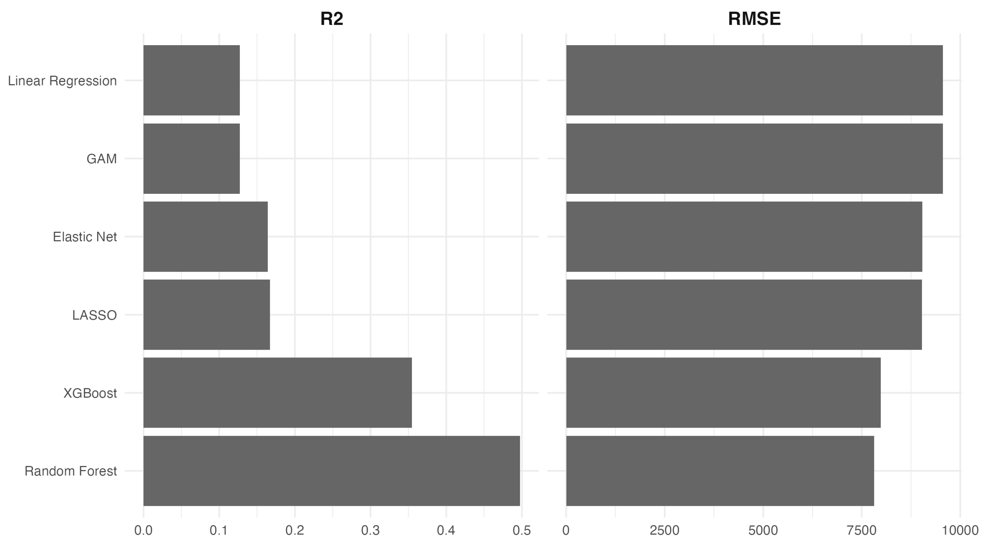
To complement the inferential spatial models and explore potential non-linearities and high-order interactions. Out-of-sample performance comparisons based on root mean squared error (RMSE) and pseudo-R2 are visualized in Figure 2. While XGBoost did not yield the lowest RMSE, it remained among the top-performing models and was selected for further analysis due to its interpretability and capacity to detect threshold interactions.
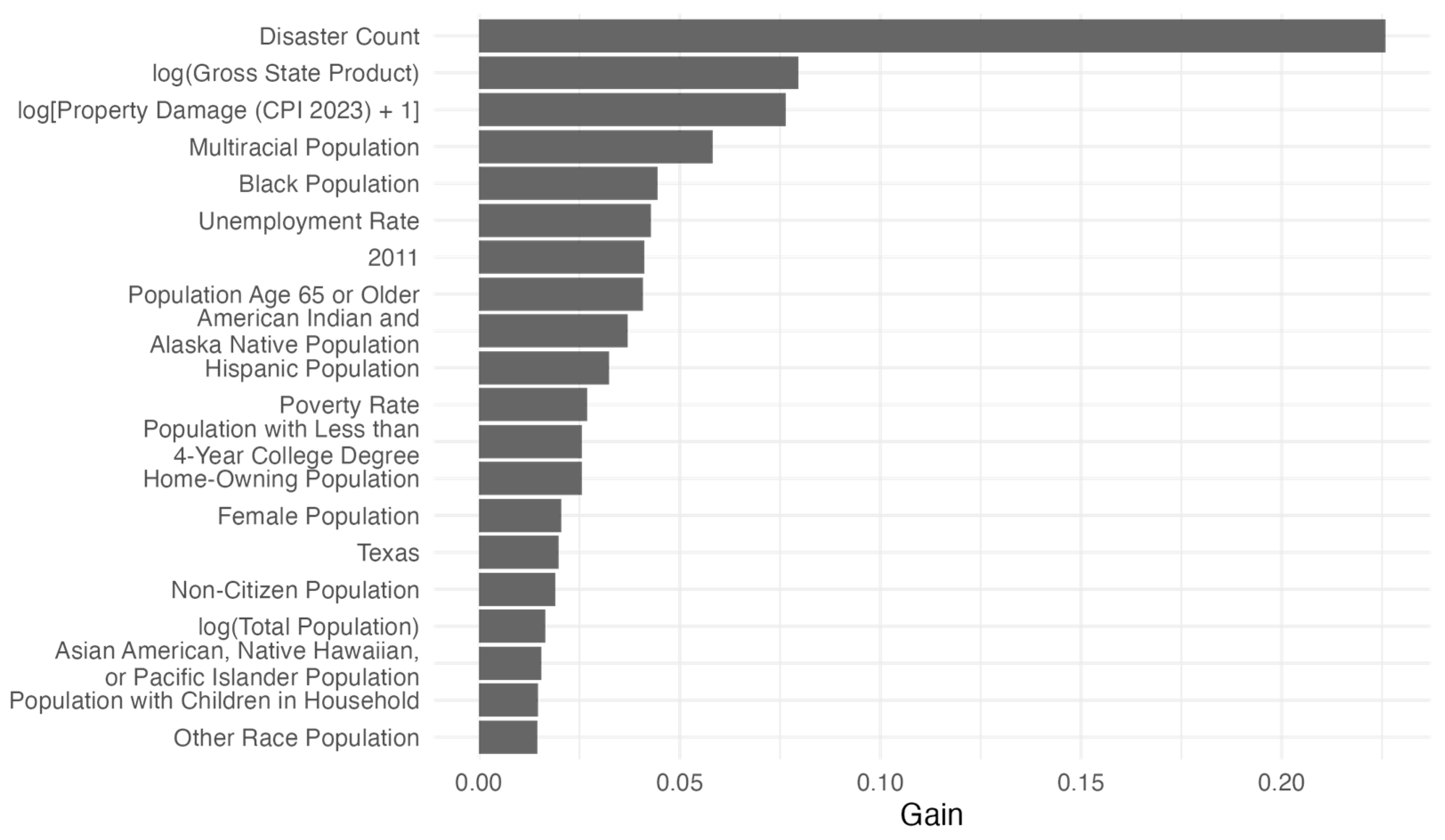
Using one of the best-performing XGBoost model, we examined feature importance (average Gain) to identify the most influential predictors of IHP expenditure per recipient (Figure 3). Although Random Forest slightly led on hold-out metrics, we selected XGBoost because gradient-boosted trees fit stage-wise additive models with explicit regularization and a tunable interaction depth, allowing us to capture complex nonlinear effects and interactions with better control over generalization. We tuned XGBoost with a randomized search over explicit regularization and interaction-depth parameters on the training data only. In each of 50 trials, we drew a 20 percent validation split from the training set, trained up to 5000 boosting rounds using the fast histogram tree builder, and applied early stopping (200 rounds) on the validation RMSE. The search varied learning rate (η), maximum depth (2–6), minimum child weight (1–16), subsample (0.60–1.00), column sample by tree (0.60–1.00), gamma (0–5), L2 (lambda, 0.1–10), and L1 (alpha, 0 or ~1 × 10⁻⁶–10). We selected the configuration with the lowest validation RMSE, refit on the full training set using the early-stopping–selected number of rounds and then evaluated once on the untouched test set. Selected hyperparameters were η = 0.021, maximum depth = 6, minimum child weight = 4, subsample = 0.78, column sample by tree = 0.64, gamma = 4.68, lambda = 1.28, and alpha = 0.000007. All runs used a fixed seed for reproducibility.
Disaster count dominates the ranking by a wide margin, followed by scale indicators—log(gross state product) and log[property damage (CPI-2023) + 1]—with multiracial and Black population shares, the unemployment rate, and the 2011-year indicator also in the upper tier. Mid-ranked predictors include population age 65+, American Indian and Alaska Native share, and Hispanic share. Lower-ranked signals include the poverty rate, population with less than a 4-year college degree, home-owning population, female share, the Texas state dummy, non-citizen share, log(total population), Asian American, Native Hawaiian, or Pacific Islander share, population with children in household, and other race share.
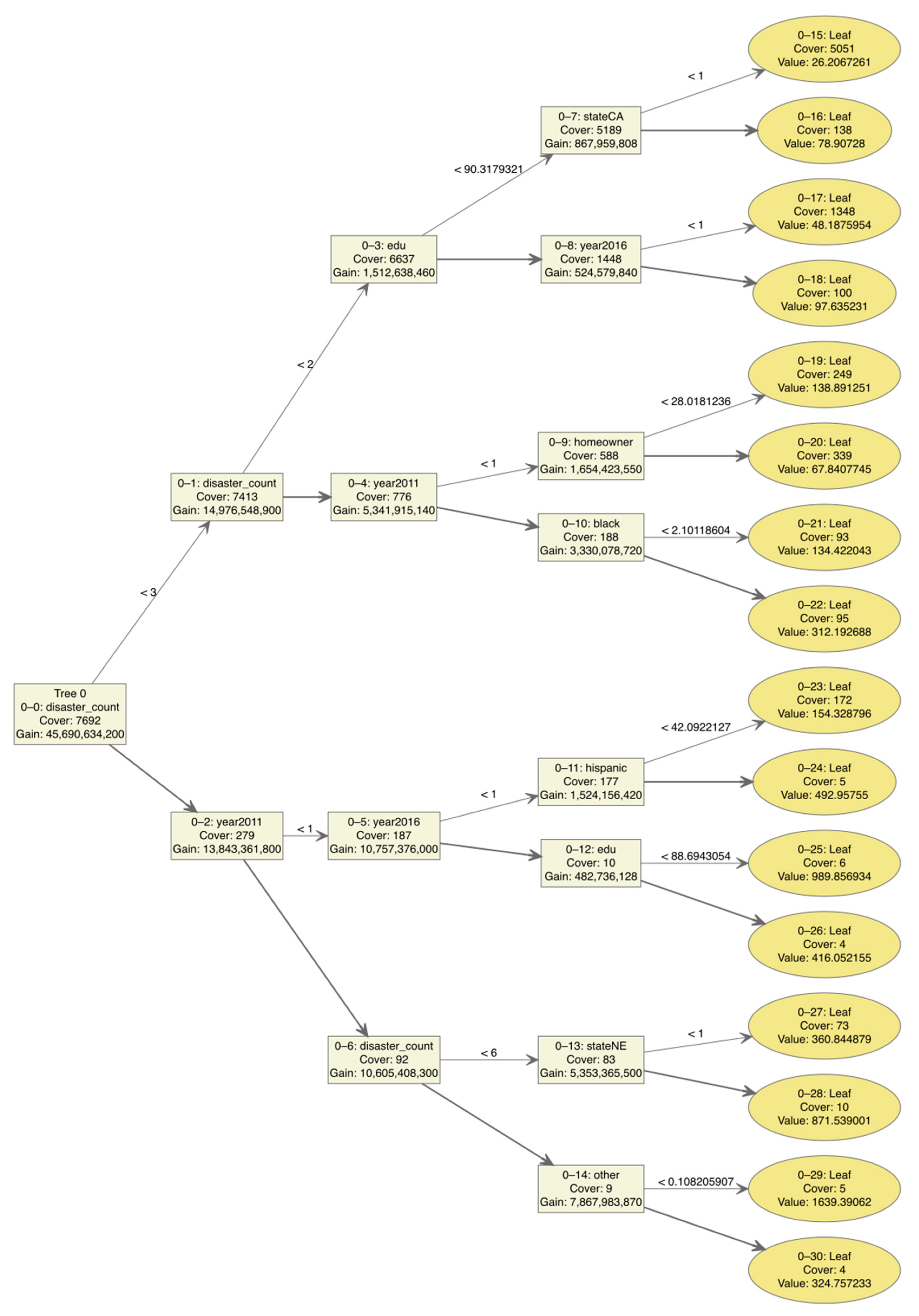
Beyond variable importance, XGBoost enabled the detection of complex, non-linear threshold effects and interaction structures often obscured in traditional regression. Figure 4 visualizes a representative decision tree trimmed to five layers from the XGBoost ensemble (the larger tree can be made available upon request). In this boosted tree, the leaf “value” is the amount this tree adds to the model’s raw prediction (scaled by the learning rate); larger positive values indicate a bigger upward adjustment to predicted IHP aid, while smaller values indicate a smaller adjustment. The root split is on the 2011-year indicator (corresponding with Hurricane Irene), separating that year from all others. On the non-2011 branch, logged property damage is the next key splitter; within lower-damage cases, the tree differentiates by state (e.g., California, Oklahoma) and by subsequent year indicators (e.g., 2016, 2021), producing the largest positive adjustments. On the 2011 branch, the tree partitions by state (e.g., Texas, Nebraska) and property damage, with later nodes involving unemployment and multiracial share.
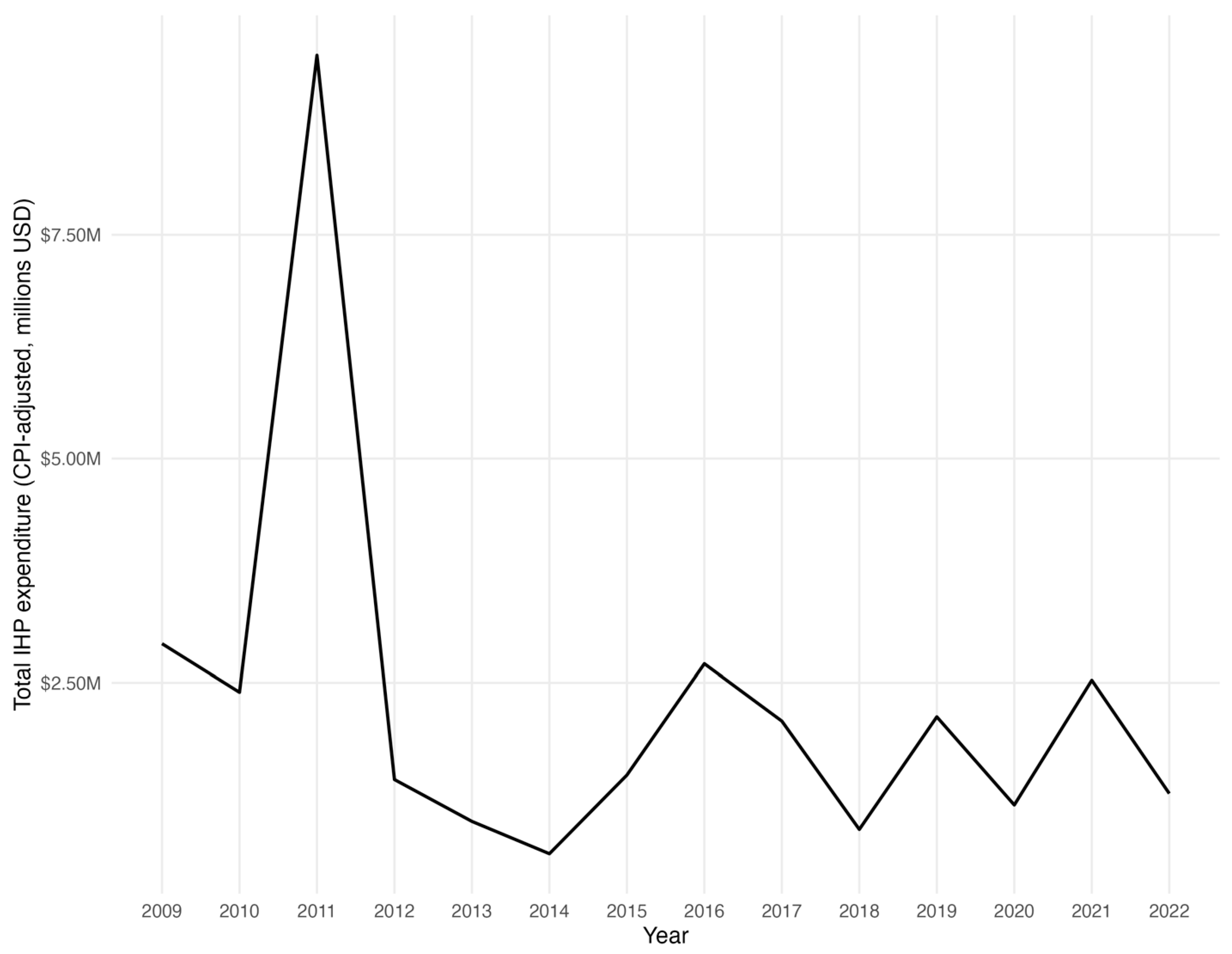
This structure highlights interactions among time, space, damages, and labor-market conditions, with the multiracial share appearing only on a downstream branch. As a single illustrative tree from the ensemble, it should not be over-interpreted as evidence of demographic tipping points; other trees might capture complementary patterns. Given the apparent importance of 2011, we conducted a sensitivity analysis (Appendix C, Table A4) that reports the RMSE and R2 of the model estimated with and without 2011, and we include a figure of IHP expenditure per recipient over time (Appendix C, Figure A2). The difference in fit is modest: the model including 2011 has a higher R2, and there is a clear spike in expenditure for that year, indicating its importance.
Read together, the space-time and machine learning approaches tell a coherent story. Both highlight exposure and time as the primary drivers of per-recipient IHP aid. However, the STDM isolates regional externalities—notably a negative neighboring effect for Hispanic share and a positive neighboring effect for poverty and population size—that machine learning treats as comparatively low-gain once broader location/time signals and nonlinearity are accounted for. Conversely, machine learning surfaces interaction and threshold structure (unemployment × damage within low-disaster regimes; year-specific shocks within high-disaster regimes) that the STAR/STDM does not model directly. In short, the space–time models explain where effects come from (direct vs. spillover), while machine learning clarifies how they operate (thresholds and interactions); the joint picture strengthens the conclusion that while sustained differences in aid are tied to sociodemographic features of social vulnerability, they are tied more to exposure, timing, and regional administrative context.

4. Discussion

This study asked whether per-recipient IHP allocations exhibit systematic space–time patterning and non-linear interactions and how those patterns relate to local composition, hazard exposure, and regional context. Read through a climate justice and adaptation lens, the results indicate that IHP operates like an event-responsive, regionally mediated social assistance program within the U.S. ecowelfare state. The space–time models show strong positive own-county disaster effects alongside negative neighboring disaster effects, consistent with administrative congestion when multiple counties are hit at once. In our models, disaster property damage is no longer a significant predictor once we account for the frequency and timing of events. This suggests that, for adaptation, how often and when hazards occur may matter more than the cost of any single event.
These results both nuance and help reconcile a literature that documents inequitable disaster aid and recovery outcomes. Existing studies frequently report penalties for marginalized groups in FEMA programs and widening racialized wealth gaps after disasters (e.g., [1,4,6,7]). By modeling space and time simultaneously, we qualify that picture. Most racial/immigration shares do not show robust direct associations with per-recipient IHP at the county level once spatial–temporal dependence is accounted for. Two patterns remain salient for climate justice—a consistent direct shortfall for counties with larger multiracial populations, and a negative neighboring (spillover) effect associated with Hispanic composition, whereby higher Hispanic shares in surrounding counties are linked to lower local aid even when own-county composition is held constant. The underlying mechanisms for this funding may be regional shortfalls in Spanish-language call-center, inspection, and case-processing capacity during multi-county surges for Hispanic households or verification rules that disadvantage multiracial households disproportionately living in rental and multifamily housing. At the same time, poverty and population size show positive neighboring effects, consistent with regional salience and scale. In ecowelfare terms, apparent “direct” penalties identified in cross-sections may reflect unmodeled regional spillovers that become visible in a space–time framework—one plausible mechanism behind the cumulative disparities highlighted by Howell & Elliott [7]. In FEMA’s regionally coordinated post-disaster operations, shared inspections, case processing, and language-access pipelines provide potential channels for such contextual spillovers, so demographic pressure in adjacent counties can depress local awards even when own-county composition is held constant.
Viewed through institutional design, our findings align with long-standing critiques that centralized eligibility and inspection systems can maladaptively ration relief during clustered events [13,14]. The negative neighboring disaster effect reads as an operational bottleneck in inspections and case processing—consistent with oversight concerns about capacity, discretion, and inconsistent implementation [17,18,20]. The Hispanic neighboring penalty coheres with evidence on documentation and language barriers in federal programs, especially for renters and mixed-status households [4,15,16]. Conversely, the positive direct association under Democratic governors might best be read as a state-capacity signal rather than partisanship, echoing accounts that intergovernmental coordination and administrative infrastructure condition how quickly safety-nets flow [17,18].
The machine learning results reinforce this interpretation. XGBoost ranks disaster count far above other predictors, followed by scale indicators—log(GSP) and log(property damage)—with multiracial and Black population shares, unemployment, and the 2011-year indicator in the next tier. A representative tree has a root split in 2011, then partitions on logged property damage and state context (e.g., California, Oklahoma), with additional year dummies (2016, 2021) and unemployment appearing downstream. This pattern suggests that timing, damage scale, and regional administrative context shape awards, consistent with the space–time results. Notably, poverty does not drive this tree, and racial composition appears only on a downstream branch, underscoring that demographic effects are often indirect and context-conditioned, whereas hazard frequency, damage severity, and administrative context carry the greatest predictive weight.
Taken together, our findings point to a troubling alignment for climate justice and adaptation. U.S. counties with greater vulnerability to climate risk remain systematically underfunded, and these funding gaps exhibit strong spatial and temporal dependencies. This persistent pattern of stratification signals not just local administrative limitations but a broader structural bias embedded in ecowelfare. As the U.S. debates whether to further devolve climate adaptation responsibilities to state and local governments [32], this study underscores the risks of decoupling federal oversight from a rapidly evolving geography of climate risk and adaptation.
These patterns translate into policy levers. Because regional surges appear to suppress local aid even where need is high, surge-capacity (the ability to handle high volumes of claims during clustered disasters) investments should be treated as resilience infrastructure. The Hispanic neighboring penalty may signal a regional gap in procedural justice; durable language-access pathways, navigator programs, and community-based application support should be deployed across multi-county clusters rather than piecemeal [4,15]. Moreover, the persistent multiracial shortfall warrants internal review to identify points of administrative attrition. And because higher aid under Democratic governors likely reflects implementation capacity, federal actors should promulgate coordination standards that establish minimum implementation thresholds in lower-capacity states irrespective of political control [17,18].
Several limitations qualify our conclusions and suggest directions for future research. These data are observational and derived from administrative sources, so unmeasured, time-varying differences in administrative capacity may lead to measurement error. Moreover, because the data are aggregated to the county level, we cannot examine how individuals’ demographic characteristics affect aid; our results reflect relationships with county composition rather than individual-level effects. Future work should aim for causality (e.g., event-study or dynamic treatment around large disasters), administrative process data to map bottlenecks, and spillover definitions that track administrative boundaries (e.g., FEMA regions). For machine learning, global explanation tools (e.g., SHAP values, partial dependence plots) can formalize thresholds and interactions, while heterogeneous-effects and spatial varying-coefficient models can identify where spillovers are strongest and who benefits least.

5. Conclusions

This study shows that FEMA’s Individuals and Households Program (IHP) operates as an event-driven, regionally mediated instrument of climate adaptation, not a need-neutral entitlement. Using space–time econometrics and machine learning, we find that per-recipient aid tracks disaster frequency far more than damage intensity, and that allocations are shaped by spillovers: aid rises with a county’s own events but falls when neighboring counties are simultaneously hit—evidence of regional congestion. Direct sociodemographic penalties are limited once spatial and temporal dependence are modeled, with two notable patterns: a persistent direct shortfall for counties with larger multiracial populations and a negative neighboring effect associated with Hispanic composition. We also detect positive neighboring effects of poverty and population scale, consistent with regional salience and capacity dynamics, and a positive direct association under Democratic governors that we interpret as differences in state capacity rather than partisanship.
Our findings suggest that inequities in the U.S. ecowelfare state arise less from a county’s own social composition than from regional context, administrative capacity, and the timing and clustering of hazards. For climate justice and adaptation, this implies that resilience hinges on building regional capacity, coordinating local–national implementation, and ensuring equitable access to programs.

Author Contributions

C.T.B. developed the conceptualization, methodology, data collection, data analysis, visualization, and writing; Y.-L.C. assisted with interpretation and review. All authors have read and agreed to the published version of the manuscript.

Funding

This research received no external funding.

Data Availability Statement

All data sources are detailed in Table 1. All data are publicly available except for SHELDUS.

Conflicts of Interest

The authors declare no conflicts of interest.

Appendix A

Table A1. SKTDM Sensitivity Analysis.
Spearman vs. BaselineTop Decile Overlap
75 km, 1 year0.9850.748
75 km, 2 years0.9860.764
75 km, 3 years0.9830.764
100 km, 1 year0.9940.9
100 km, 3 years0.9980.965
150 km, 1 year0.950.764
150 km, 2 years0.9650.759
150 km, 3 years0.9660.753
Note. Baseline: 100 km, 2 years.
Figure A1. Kernel-smoothed IHP aid per recipient, 5-year period.
Climate 13 00244 g0a1

Appendix B

Table A2. Sensitivity Analysis: STAR with Spatial Weights.
MainNearest NeighborsKilometers
46100150
βββββ
Disaster Count4994.898 ***
(104.812)
5046.924 ***
(105.915)
5045.105 ***
(105.988)
−70.819 *
(38.044)
−69.490 *
(38.077)
AANHPI−69.910
(37.940)
−96.618 **
(38.284)
−94.208 **
(38.264)
0.194
(15.984)
−0.177
(16.000)
AIAN2.133
(15.942)
−4.498
(16.084)
−3.101
(16.075)
−2.802
(7.708)
−1.470
(7.716)
Black−2.567
(7.688)
−1.008
(7.758)
−1.538
(7.754)
−21.680*
(11.786)
−15.128
(11.847)
Hispanic−21.725
(11.716)
−44.785 ***
(11.789)
−41.022 ***
(11.786)
−140.067 **
(68.268)
−151.635 **
(68.326)
Multiracial−136.112 *
(68.099)
−156.900 **
(68.675)
−150.955 **
(68.637)
438.007
(376.245)
432.187
(376.538)
Other Race458.727
(375.335)
428.075
(378.737)
441.952
(378.513)
−53.317
(34.159)
−54.525
(34.185)
Age 65 or Older−52.313
(34.075)
−51.512
(34.385)
−49.614
(34.364)
28.998
(17.796)
27.020
(17.810)
Less than 4-Years of College28.902
(17.751)
37.654 **
(17.925)
34.729 *
(17.914)
39.901
(38.948)
35.347
(39.011)
Non-Citizen 44.244
(38.840)
73.511 *
(39.175)
68.958 *
(39.154)
−27.037
(20.422)
−25.877
(20.441)
Poverty−30.751
(20.367)
−16.687
(20.546)
−17.487
(20.534)
18.052
(42.590)
11.744
(42.624)
Female 26.417
(42.487)
12.286
(42.880)
17.574
(42.856)
−9.480
(36.354)
−2.291
(36.401)
Homeowner−7.312
(36.263)
−14.051
(36.590)
−14.840
(36.569)
−89.696
(66.327)
−98.931
(66.402)
Children in Household−101.694
(66.160)
−75.579
(66.753)
−76.760
(66.714)
139.168
(93.562)
146.691
(93.628)
log(Total Population)141.609
(93.360)
213.884 **
(94.243)
201.619 **
(94.191)
131.090 ***
(45.972)
124.276 ***
(46.003)
Unemployment131.584 **
(45.866)
142.066 ***
(46.278)
141.136 ***
(46.250)
4999.487 ***
(104.593)
5010.380 ***
(104.615)
log(Gross State Product)−1828.480
(1574.036)
−1502.057
(1588.487)
−1559.115
(1587.558)
−1780.553
(1577.809)
−1774.104
(1579.024)
Democratic Governor
     Non-Democrat (reference)---------------
     Democrat1046.615 ***
(196.914)
1052.074 ***
(198.724)
1058.651 ***
(198.603)
1041.128 ***
(197.394)
1027.789 ***
(197.551)
Metro Status
     Metro areas of 1 million or more (reference)---------------
     Metro areas of 250,000 to 1 million−604.716 *
(237.200)
−546.661 **
(239.293)
−547.031 **
(239.146)
−610.183 **
(237.738)
−580.643 **
(237.943)
     Metro areas of fewer than 250,000−104.548
(268.935)
−5.547
(271.326)
−17.537
(271.164)
−69.262
(269.563)
−15.536
(269.783)
     Non-metro areas of fewer than 250,000 population−201.878
(261.487)
−96.305
(263.722)
−111.055
(263.583)
−198.021
(262.019)
−156.854
(262.208)
log(Property Damage + 1)−6.717
(13.518)
−7.685
(13.640)
−7.321
(13.632)
−6.419
(13.551)
−7.223
(13.562)
Intercept11,869.054
(17,095.697)
8798.265
(17,253.029)
9405.585
(17,242.894)
12,333.915
(17,136.323)
12,346.179
(17,149.623)
AIC260,506.323260,674.036260,663.081260,547.808260,560.129
BIC261,146.377261,314.09261,303.135261,187.861261,200.182
Log Likelihood−130,167.16−130,251.02−130,245.54−130,187.9−130,194.06
ρ0.3360.0000.0500.3530.452
Residual Variance53,623,809.954,601,863.854,537,459.153,885,391.253,969,685.9
Note. Year and state fixed effects excluded from table. * p < 0.05, ** p < 0.01, *** p < 0.001.
Table A3. Sensitivity Analysis: STDM with Spatial Weights.
MainNearest NeighborsKilometers
46100150
βθβθβθβθβθ
Disaster Count5197.283 ***
(106.291)
−2789.291 ***
(360.917)
5651.366 ***
(109.559)
−2868.246 ***
(170.091)
5651.411 ***
(109.879)
−3397.642 ***
(202.485)
5069.603 ***
(105.376)
−2376.050 ***
(603.092)
5070.861 ***
(105.076)
−3380.173 ***
(962.521)
AANHPI−44.819
(50.132)
−105.774
(87.097)
103.951 *
(58.247)
−198.399 ***
(67.615)
80.279
(54.279)
−179.017 ***
(68.093)
−65.799
(45.275)
−119.318
(92.518)
−49.392
(42.890)
−220.027 *
(121.131)
AIAN18.387
(19.848)
−60.163
(38.490)
27.837
(105.296)
−129.926
(117.147)
−14.664
(95.129)
−88.560
(109.948)
3.160
(20.360)
−1.517
(36.350)
−2.686
(18.924)
10.701
(46.655)
Black−8.330
(11.910)
6.627
(18.466)
67.556 **
(29.485)
−96.643 ***
(33.233)
38.921
(25.453)
−77.224 **
(32.917)
−17.696 *
(10.520)
54.516 **
(22.662)
−14.070
(9.782)
50.118
(32.481)
Hispanic2.532
(22.830)
−62.354 *
(28.475)
−32.025
(27.391)
32.862
(28.426)
−12.489
(22.476)
13.814
(24.095)
−12.391
(23.012)
−28.831
(30.091)
−2.597
(21.042)
−55.438
(34.074)
Multiracial−176.085 *
(83.611)
150.078
(153.974)
−15.462
(34.204)
−45.964
(35.805)
−24.900
(31.438)
−33.118
(34.125)
−179.734 **
(80.384)
145.294
(177.629)
−205.359 ***
(77.776)
209.658
(230.114)
Other Race488.658
(391.721)
−563.271
(1082.574)
−118.788
(94.613)
6.497
(115.587)
−141.447
(94.148)
39.288
(125.846)
484.947
(388.888)
−1209.574
(1574.844)
438.950
(384.951)
−5452.111 *
(2859.205)
Age 65 or Older−56.295
(41.594)
54.094
(86.634)
706.415 *
(423.661)
−1008.755
(668.271)
737.739 *
(428.891)
−1167.566
(726.282)
−69.647 *
(38.419)
−1.873
(107.375)
−73.589 **
(37.044)
−165.433
(164.091)
Less than 4-Years of College5.597
(21.832)
37.954
(43.529)
25.406
(39.279)
33.404
(43.670)
18.109
(35.143)
36.233
(41.130)
13.459
(20.050)
38.816
(58.586)
12.946
(19.429)
109.241
(88.013)
Non-Citizen 12.940
(52.428)
107.339
(86.090)
39.138
(72.474)
72.824
(78.335)
46.369
(67.887)
74.276
(78.740)
23.842
(52.157)
98.496
(94.066)
18.754
(48.919)
146.581
(125.519)
Poverty−45.781
(24.982)
113.858 *
(50.485)
−48.122
(31.126)
55.835
(36.456)
−47.745
(30.064)
63.140 *
(38.135)
−30.458
(23.720)
37.706
(61.711)
−23.730
(22.987)
−62.352
(91.359)
Female 41.883
(46.100)
−166.967
(121.593)
−54.967
(64.645)
38.603
(80.178)
−35.085
(59.060)
15.804
(80.135)
24.308
(44.396)
−77.265
(168.935)
20.057
(43.707)
184.630
(269.877)
Homeowner38.879
(42.754)
−97.026
(89.497)
−50.467
(53.751)
84.179
(64.977)
−60.064
(51.376)
109.680
(66.921)
−0.440
(39.791)
51.217
(117.025)
10.650
(38.785)
59.565
(185.366)
Children in Household−172.265 *
(71.417)
174.827
(195.235)
−58.518
(80.807)
−52.698
(108.627)
−75.259
(79.574)
−11.903
(118.242)
−118.689 *
(69.619)
−280.777
(267.804)
−131.258 *
(68.726)
−544.267
(434.138)
log(Total Population)98.264
(118.144)
486.705 *
(238.940)
611.361 ***
(224.594)
−310.443
(248.624)
379.598 **
(185.599)
−54.997
(219.873)
78.166
(108.942)
987.932 ***
(295.795)
89.243
(105.441)
769.905 *
(443.712)
Unemployment137.225 **
(50.899)
−129.130
(128.920)
205.181 ***
(52.773)
−105.636
(70.718)
200.422 ***
(52.857)
−129.914
(79.651)
136.648 ***
(49.931)
−119.091
(156.742)
113.140 **
(48.569)
217.061
(225.472)
log(Gross State Product)−1727.527
(1581.226)
171.452
(760.950)
−818.660
(1614.208)
−1832.808
(3421.237)
−736.927
(1610.355)
−5393.370
(4128.130)
−1691.138
(1591.418)
−676.786
(926.739)
−1790.384
(1590.433)
−2207.612
(1377.546)
Democratic Governor
     Non-Democrat (reference)------------------------------
     Democrat1031.460 ***
(196.574)
−89.261
(1074.730)
887.480 ***
(199.588)
−131.610
(444.795)
934.310 ***
(199.516)
−307.240
(537.862)
1008.381 ***
(197.575)
−542.964
(1446.450)
1004.364 ***
(197.788)
861.702
(2294.675)
Metro Status
     Metro areas of 1 million or more (reference)------------------------------
     Metro areas of 250,000 to 1 million−334.708
(397.011)
114.467
(578.038)
−1451.538
(1027.345)
1174.191
(1047.881)
−1548.485 **
(767.141)
1349.020 *
(800.145)
−636.902 **
(310.204)
970.023
(678.253)
−449.817 *
(267.013)
1317.258
(981.910)
     Metro areas of fewer than 250,000−135.745
(417.129)
704.648
(662.455)
−1692.299 *
(967.286)
1825.810 *
(995.643)
−878.930
(756.731)
1050.473
(802.148)
−141.399
(329.059)
1671.865 **
(797.029)
158.900
(294.517)
1016.165
(1189.490)
     Non-metro areas of fewer than 250,000 population−10.134
(375.801)
332.794
(660.445)
−1296.351
(829.115)
1377.659
(867.063)
−934.328
(655.664)
1191.565 *
(717.973)
−313.222
(310.893)
2269.579 **
(884.058)
−104.755
(283.684)
2902.894 **
(1396.637)
log(Property Damage + 1)−11.165
(13.555)
11.096
(61.427)
−8.870
(13.510)
−23.941
(27.778)
−9.762
(13.493)
−7.226
(33.140)
−10.341
(13.614)
−25.564
(82.124)
−9.403
(13.609)
144.560
(125.349)
Intercept12,366.147
(17,626.566)
22,855.862
(42,625.090)
60,166.317
(49,720.086)
15,793.473
(17,559.226)
15,345.563
(17,992.076)
AIC260,521.588 260,460.01 260,456.262 260,599.662 260,600.915
BIC261,771.925 261,688.02 261,691.715 261,849.999 261,851.252
Log Likelihood−130,092.79 −130,065.005 −130,062.131 −130,131.83 −130,132.46
ρ0.347 0.057 0.106 0.332 0.382
Residual Variance52,977,052 52,985,121.65 52,913,033.78 53,430,034.1 53,489,456.4
Note. Year and state fixed effects excluded from table. * p < 0.05, ** p < 0.01, *** p < 0.001.

Appendix C

Table A4. Sensitivity Analysis: XGBoost with and without 2011.
Test RMSEValidation RMSETest R2
All years7214.8415430.3380.466
Exclude 20118723.1874482.4110.220
Figure A2. IHP Expenditure Per Recipient Over Time.
Climate 13 00244 g0a2

References

  1. Drakes, O.; Tate, E.; Rainey, J.; Brody, S. Social vulnerability and short-term disaster assistance in the United States. Int. J. Disaster Risk Reduct. 2021, 53, 102010. [Google Scholar] [CrossRef]
  2. Emrich, C.T.; Aksha, S.K.; Zhou, Y. Assessing distributive inequities in FEMA’s disaster recovery assistance fund allocation. Int. J. Disaster Risk Reduct. 2022, 74, 102855. [Google Scholar] [CrossRef]
  3. Brown, C.T.; Chang, Y.L. Ecosocial policy and the social risks of climate change: Foundations of the US ecosocial safety net. J. Soc. Policy 2024, 1–20. [Google Scholar] [CrossRef]
  4. Domingue, S.J.; Emrich, C.T. Social vulnerability and procedural equity: Exploring the distribution of disaster aid across counties in the United States. Am. Rev. Public Adm. 2019, 49, 897–913. [Google Scholar] [CrossRef]
  5. Han, Y.; Jia, H.; Xu, C.; Bockarjova, M.; van Westen, C.; Lombardo, L. Unveiling spatial inequalities: Exploring county-level disaster damages and social vulnerability on public disaster assistance in contiguous US. J. Environ. Manag. 2024, 351, 119690. [Google Scholar] [CrossRef]
  6. Muñoz, C.E.; Tate, E. Unequal recovery? Federal resource distribution after a Midwest flood disaster. Int. J. Environ. Res. Public Health 2016, 13, 507. [Google Scholar] [CrossRef] [PubMed]
  7. Howell, J.; Elliott, J.R. Damages done: The longitudinal impacts of natural hazards on wealth inequality in the United States. Soc. Probl. 2019, 66, 448–467. [Google Scholar] [CrossRef]
  8. Brown, C.T.; Nepomnyashcy, L.; Patel, A.S. Is the U.S. ecosocial safety net inequitable? Comparing the Individuals and Households and National Flood Insurance programs. In Proceedings of the 46th Annual Meeting of the Association for Public Policy Analysis and Management, National Harbor, MD, USA, 21–23 November 2024. [Google Scholar]
  9. Intergovernmental Panel on Climate Change. Climate Change 2023: Synthesis Report; IPCC: Geneva, Switzerland, 2023. [Google Scholar] [CrossRef]
  10. Schlosberg, D.; Collins, L.B. From environmental to climate justice: Climate change and the discourse of environmental justice. WIREs Clim. Change 2014, 5, 359–374. [Google Scholar] [CrossRef]
  11. Gough, I. Climate change, social policy, and global governance. J. Int. Comp. Soc. Policy 2013, 29, 185–203. [Google Scholar] [CrossRef]
  12. Hirvilammi, T.; Häikiö, L.; Johansson, H.; Koch, M.; Perkiö, J. Social policy in a climate emergency context: Towards an ecosocial research agenda. J. Soc. Policy 2023, 52, 1–23. [Google Scholar] [CrossRef]
  13. Bolin, B.; Kurtz, L.C. Race, class, ethnicity, and disaster vulnerability. In Handbook of Disaster Research; Rodríguez, H., Donner, W., Trainor, J., Eds.; Springer: Cham, Switzerland, 2018. [Google Scholar] [CrossRef]
  14. Rivera, J.D.; Miller, D.S. Continually neglected: Situating natural disasters in the African American experience. J. Black Stud. 2007, 37, 502–522. [Google Scholar] [CrossRef]
  15. Lamba-Nieves, D.; Santiago-Bartolomei, R. Who gets emergency housing relief? An analysis of FEMA individual assistance data after Hurricane María. Hous. Policy Debate 2023, 33, 1146–1166. [Google Scholar] [CrossRef]
  16. Raker, E.J.; Woods, T. Disastrous burdens: Hurricane Katrina, federal housing assistance, and well-being. RSF 2023, 9, 122–143. [Google Scholar] [CrossRef]
  17. Congressional Research Service. FEMA’s Individuals and Households Program (IHP)—Implementation and Considerations for Congress; R47015; CRS: Washington, DC, USA, 2021. Available online: https://www.congress.gov/crs_external_products/R/PDF/R47015/R47015.1.pdf (accessed on 20 October 2025).
  18. U.S. Government Accountability Office. Disaster Assistance: Updated FEMA Guidance Could Better Help Communities Apply for Individual Assistance; GAO-25-106768; GAO: Washington, DC, USA, 2025. Available online: https://www.gao.gov/products/gao-25-106768 (accessed on 20 October 2025).
  19. Federal Emergency Management Agency. Individual Assistance Program and Policy Guide, Version 1.1; FP 104-009-03; FEMA: Washington, DC, USA, 2021. Available online: https://www.fema.gov/sites/default/files/documents/fema_iappg-1.1.pdf (accessed on 20 October 2025).
  20. U.S. Government Accountability Office. Disaster Assistance: Additional Actions Needed to Strengthen FEMA’s Individuals and Households Program; GAO-20-503; GAO: Washington, DC, USA, 2020. Available online: https://www.gao.gov/products/gao-20-503 (accessed on 20 October 2025).
  21. Simpson, N.P.; Williams, P.A.; Mach, K.J.; Berrang-Ford, L.; Biesbroek, R.; Haasnoot, M.; Segnon, A.C.; Campbell, D.; Musah-Surugu, J.I.; Joe, E.T.; et al. Adaptation to compound climate risks: A systematic global stocktake. iScience 2023, 26, 105926. [Google Scholar] [CrossRef]
  22. Elliott, J.R.; Howell, J. Beyond disasters: A longitudinal analysis of natural hazards’ unequal impacts on residential instability. Soc. Forces 2017, 95, 1181–1207. [Google Scholar] [CrossRef]
  23. Boustan, L.P.; Kahn, M.E.; Rhode, P.W.; Yanguas, M.L. The effect of natural disasters on economic activity in US counties: A century of data. J. Urban Econ. 2020, 118, 103257. [Google Scholar] [CrossRef]
  24. McIntosh, M.F. Measuring the labor market impacts of Hurricane Katrina migration: Evidence from Houston, Texas. Am. Econ. Rev. 2008, 98, 54–57. [Google Scholar] [CrossRef]
  25. Varano, S.P.; Schafer, J.A.; Cancino, J.M.; Decker, S.H.; Greene, J.R. A tale of three cities: Crime and displacement after Hurricane Katrina. J. Crim. Justice 2010, 38, 42–50. [Google Scholar] [CrossRef]
  26. Dupor, B.; McCrory, P.B. A cup runneth over: Fiscal policy spillovers from the 2009 Recovery Act. Econ. J. 2018, 128, 1476–1508. [Google Scholar] [CrossRef]
  27. Auerbach, A.J.; Gorodnichenko, Y.; Murphy, D. Local Fiscal Multipliers and Fiscal Spillovers in the United States. National Bureau of Economic Research Working Paper No. 25457; NBER: Cambridge, MA, USA, 2019; Available online: https://www.nber.org/system/files/working_papers/w25457/w25457.pdf (accessed on 20 October 2025).
  28. Berry, F.S.; Berry, W.D. State lottery adoptions as policy innovations: An event history analysis. Am. Polit. Sci. Rev. 1990, 84, 395–415. [Google Scholar] [CrossRef]
  29. Baybeck, B.; Berry, W.D.; Siegel, D.A. A strategic theory of policy diffusion via intergovernmental competition. J. Polit. 2011, 73, 232–247. [Google Scholar] [CrossRef]
  30. Abramovitz, M. Regulating the Lives of Women: Social Welfare Policy from Colonial Times to the Present; Routledge: London, UK, 2017. [Google Scholar]
  31. Chang, Y.L.; Lanfranconi, L.M.; Clark, K. Second-order devolution revolution and the hidden structural discrimination? Examining county welfare-to-work service systems in California. J. Poverty 2020, 24, 430–450. [Google Scholar] [CrossRef]
  32. Executive Order, No. 14180, Council to Assess the Federal Emergency Management Agency. Fed. Regist. 2025, 90, 8743–8745. Available online: https://www.federalregister.gov/documents/2025/01/31/2025-02173/council-to-assess-the-federal-emergency-management-agency (accessed on 20 October 2025).
  33. Diggle, P.J. Statistical Analysis of Spatial and Spatio-Temporal Point Patterns, 3rd ed.; Chapman & Hall/CRC: New York, NY, USA, 2013. [Google Scholar]
  34. Zhao, Z.; Cui, Y.; Qiu, X.; Wang, Y. A spatio-temporal kernel density estimation framework for predictive crime hotspot mapping and evaluation. ISPRS Int. J. Geo-Inf. 2021, 10, 217. [Google Scholar] [CrossRef]
  35. Shoesmith, G.L. Space–time autoregressive models and forecasting national, regional and state crime rates. Int. J. Forecast. 2013, 29, 191–201. [Google Scholar] [CrossRef]
  36. Elhorst, J.P. Dynamic spatial panels: Models, methods, and inferences. J. Geogr. Syst. 2012, 14, 5–28. [Google Scholar] [CrossRef]
  37. LeSage, J.; Pace, R.K. Introduction to Spatial Econometrics; Chapman & Hall/CRC: New York, NY, USA, 2009. [Google Scholar]
  38. Fotheringham, A.S.; Brunsdon, C.; Charlton, M. Geographically Weighted Regression: The Analysis of Spatially Varying Relationships; Wiley: New York, NY, USA, 2002. [Google Scholar]
  39. Rao, H.; Li, J.; Zhang, L.; Zhang, J. A machine learning framework for modeling post-disaster recovery time of communities. Int. J. Disaster Risk Reduct. 2021, 62, 102395. [Google Scholar]
  40. Brandenburg, C.; Bivand, R. Random forest as a generic framework for predictive modeling of spatial and spatio-temporal variables. Stoch. Environ. Res. Risk Assess. 2021, 35, 139–160. [Google Scholar]
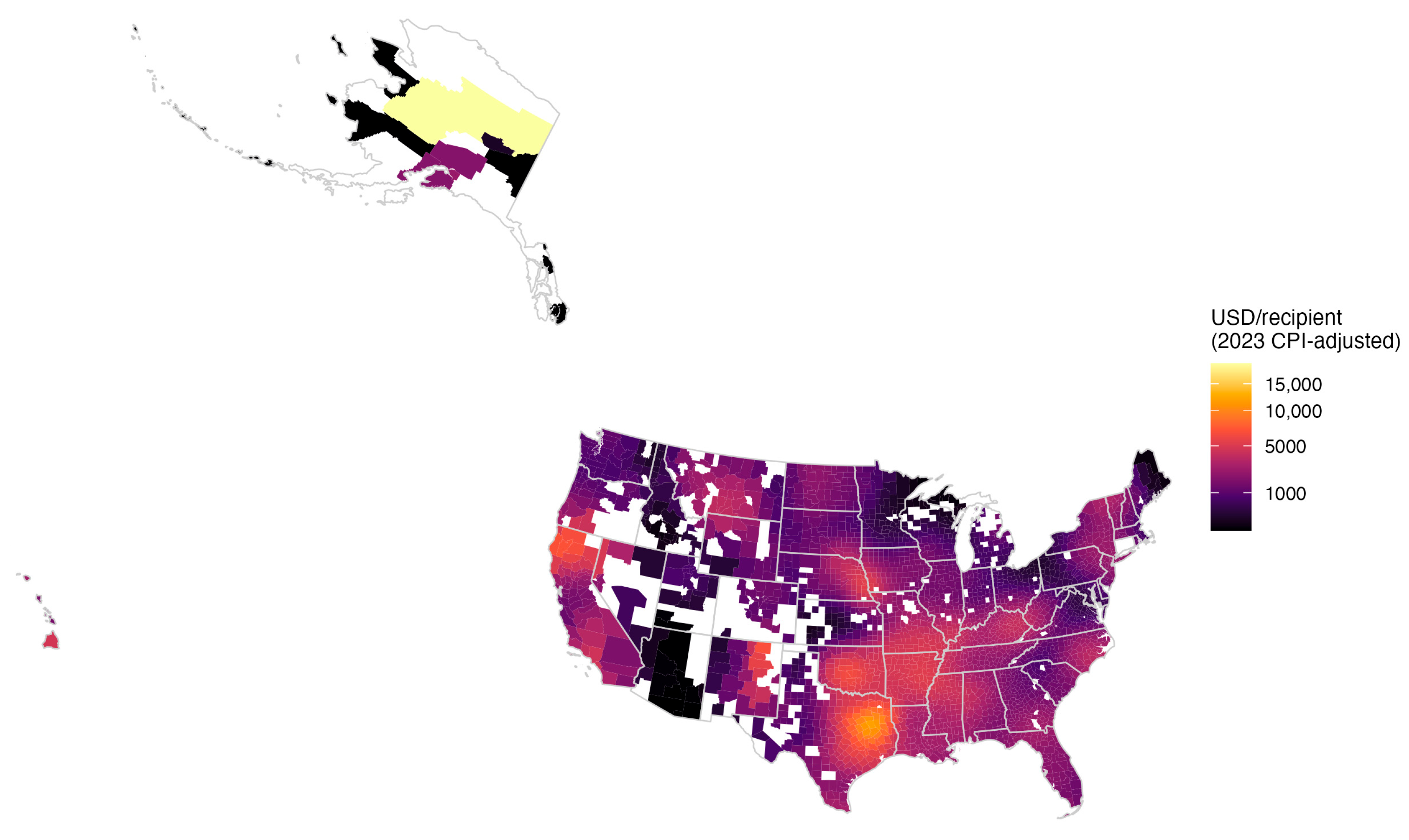
Figure 1. Kernel-smoothed IHP aid per recipient, 2009–2002.
Climate 13 00244 g001
Figure 2. Machine Learning Algorithm Comparisons.
Climate 13 00244 g002
Figure 3. XGBoost Variable Importance, Top 20.
Climate 13 00244 g003
Figure 4. XGBoost Decision Tree, Trimmed to Five Layers.
Climate 13 00244 g004
Table 1. Variable Descriptions and Sources.
VariableDescriptionSource
Dependent Variable
IHP Expenditure per RecipientThe amount of IHP funding per recipientRI-IHP
Independent Variables
AANHPI PopulationProportion of Asian American and Native Hawaiian or Pacific Islander populationACS
AIAN PopulationProportion of American Indian or Alaska Native populationACS
Black PopulationProportion of Black populationACS
Hispanic PopulationProportion of Hispanic populationACS
Multiracial PopulationProportion of multiracial populationACS
Other Race PopulationProportion of other race populationACS
Older than Age 65 PopulationProportion of population Older than Age 65ACS
Less than 4-Years of
College Population
Proportion of population with less than 4-years of collegeACS
Non-Citizen PopulationProportion of non-citizen populationACS
Poverty Rate Poverty rateACS
Female PopulationProportion of female populationACS
Children in Household. PopulationProportion of households with at least one child under the age of 18ACS
Homeowner PopulationProportion of homeowning populationACS
Total Population (in 100,000’s)Total population divided by 100,000ACS
Gross State ProductGross state product per capitaWRD
Democratic GovernorPolitical affiliation of state GovernorWRD
RuralityRural–urban continuum codesUSDA
Number of HazardsNumber of hazardsSHELDUS
Disaster Property DamageTotal property damageSHELDUS
Note. All variables aggregated by county and year.
Table 2. Descriptive Statistics.
MeanSDN
IHP Expenditure per Recipient2534.0218385.775126,23
AANHPI1.8083.555126,23
AIAN1.165.283126,23
Black11.70315.607126,23
Hispanic8.47712.575126,23
Multiracial1.9351.792126,23
Other Race0.140.212126,23
White74.77620.26126,23
Age 65 or Older16.5544.399126,23
Less than 4-Years of College84.9676.803126,23
Non-Citizen3.0473.651126,23
Poverty15.2936.168126,23
Female50.3132.039126,23
Homeowner27.3124.33126,23
Children in Household11.8171.559126,23
Total Population193,354512,982.6126,23
Unemployment6.4732.802126,23
Gross State Product540,176.1581,136.2126,23
Democratic Governor
     Non-Democrat 7829 (62%)
     Democrat 4784 (38%)
Metro Status
     Metro areas of 1 million or more 2793 (22%)
     Metro areas of 250,000 to 1 million 2118 (17%)
     Metro areas of fewer than 250,000 1556 (12%)
     Non-metro areas of fewer than 250,000 population 6156 (49%)
Disaster Count1.2050.66412,623
Disaster Property Damage72,089,151,320,293.9272,338,196,533,04112,623
Table 3. Space-Time Model Coefficients.
STARSTDM
ββθ
Disaster Count4994.898 ***
(104.812)
5197.283 ***
(106.291)
−2789.291 ***
(360.917)
AANHPI−69.910
(37.940)
−44.819
(50.132)
−105.774
(87.097)
AIAN2.133
(15.942)
18.387
(19.848)
−60.163
(38.490)
Black−2.567
(7.688)
−8.330
(11.910)
6.627
(18.466)
Hispanic−21.725
(11.716)
2.532
(22.830)
−62.354 *
(28.475)
Multiracial−136.112 *
(68.099)
−176.085 *
(83.611)
150.078
(153.974)
Other Race458.727
(375.335)
488.658
(391.721)
−563.271
(1082.574)
Age 65 or Older−52.313
(34.075)
−56.295
(41.594)
54.094
(86.634)
Less than 4-Years of College28.902
(17.751)
5.597
(21.832)
37.954
(43.529)
Non-Citizen44.244
(38.840)
12.940
(52.428)
107.339
(86.090)
Poverty−30.751
(20.367)
−45.781
(24.982)
113.858 *
(50.485)
Female26.417
(42.487)
41.883
(46.100)
−166.967
(121.593)
Homeowner−7.312
(36.263)
38.879
(42.754)
−97.026
(89.497)
Children in Household−101.694
(66.160)
−172.265 *
(71.417)
174.827
(195.235)
Log(Total Population)141.609
(93.360)
98.264
(118.144)
486.705 *
(238.940)
Unemployment131.584 **
(45.866)
137.225 **
(50.899)
−129.130
(128.920)
Log(Gross State Product)−1828.480
(1574.036)
−1727.527
(1581.226)
171.452
(760.950)
Democratic Governor
     Non-Democrat (reference)---------
     Democrat1046.615 ***
(196.914)
1031.460 ***
(196.574)
−89.261
(1074.730)
Metro Status
     Metro areas of 1 million or more (reference)---------
     Metro areas of 250,000 to 1 million−604.716 *
(237.200)
−334.708
(397.011)
114.467
(578.038)
     Metro areas of fewer than 250,000−104.548
(268.935)
−135.745
(417.129)
704.648
(662.455)
     Non-metro areas of fewer than 250,000 population−201.878
(261.487)
−10.134
(375.801)
332.794
(660.445)
Log(Property Damage + 1)−6.717
(13.518)
−11.165
(13.555)
11.096
(61.427)
Intercept11,869.054
(17,095.697)
12,366.147
(17,626.566)
AIC260,506.323260,521.588
BIC261,146.377261,771.925
Log Likelihood−130,167.16−130,092.79
ρ0.3360.347
Residual Variance53,623,809.952,977,052
Note. * p < 0.05, ** p < 0.01, *** p < 0.001. Year and state fixed effects were excluded from the table.
Disclaimer/Publisher’s Note: The statements, opinions and data contained in all publications are solely those of the individual author(s) and contributor(s) and not of MDPI and/or the editor(s). MDPI and/or the editor(s) disclaim responsibility for any injury to people or property resulting from any ideas, methods, instructions or products referred to in the content.