A Joint Specification Test for Response Probabilities in Unordered Multinomial Choice Models

Abstract

Estimation results obtained by parametric models may be seriously misleading when the model is misspecified or poorly approximates the true model. This study proposes a test that jointly tests the specifications of multiple response probabilities in unordered multinomial choice models. The test statistic is asymptotically chi-square distributed, consistent against a fixed alternative and able to detect a local alternative approaching to the null at a rate slower than the parametric rate. We show that rejection regions can be calculated by a simple parametric bootstrap procedure, when the sample size is small. The size and power of the tests are investigated by Monte Carlo experiments.

1. Introduction

Not infrequently, variables of interest in economic research are discrete and unordered, as we often find the variables that indicate the behavior or state of economic agents. Some econometric models have been developed to deal with these discrete and unordered outcomes. Above all, parametric models, such as the multinomial logit (MNL) and probit (MNP) models proposed by [1,2], respectively, are widely employed, for example, in structural econometric analysis (e.g., the economic models of automobile sales in [3,4]) and as part of econometric methods (e.g., selection bias correction of [5,6]). However, results obtained by such parametric models may be seriously misleading when the model is misspecified or poorly approximates the true model. Thus, researchers need to examine the validity of parametric assumptions as long as the assumptions are refutable from data alone.

This study proposes a new specification test that is directly applicable to any multinomial choice models with unordered outcome variables. These models set parametric assumptions on response probabilities that an option is chosen from multiple alternatives, and identical assumptions are often set for all response probabilities. Problems occur when these models do not mimic the true models, because the response probabilities and partial effects of some variables on the probabilities cannot be properly predicted. Moreover, the parameter estimation results may be misleading and their interpretation confusing. The specification test proposed here can be utilized to justify the choice of parametric models and to avoid misspecification problems.

The novelty of the test provided in this study is that it allows us to test the specifications of response probabilities jointly for all choice alternatives. Multinomial choice models with unordered outcomes consist of multiple response probabilities, each of which may be parameterized differently. This implies that one needs to test multiple null hypotheses to justify the parametric assumptions of these models. A substantial number of specification tests has been developed to test a single null hypothesis. To our knowledge, however, no joint specification tests have so far been theoretically suggested for multiple null hypotheses.

The test proposed here is based on moment conditions. We show that the test statistic is asymptotically chi-square distributed, consistent against a fixed alternative and able to detect a local alternative approaching the null at the rate of $1/\sqrt{n{h}^{q/2}}$, where q is the number of independent variables.

One eminent feature of our test is that a parametric bootstrap procedure works well to calculate the rejection region for the test statistic. Since the testing method involves nonparametric estimation, a sufficiently large sample size could be required to establish that the chi-squared distribution is a proper approximation for the distribution of the test statistic. Thus, a simple parametric bootstrap procedure to calculate rejection regions is a practical need.

A crucial point that makes parametric bootstrap work is that the orthogonality condition holds with bootstrap sampling under both the null and alternative hypotheses. This is different from the specification test for the regression function that requires the wild bootstrapping procedure to calculate the rejection region proven by [7]. It is also noteworthy that the parametric nature of the model leads to substantial savings in the computational cost of bootstrapping.

Methodologically, two different approaches have been developed to construct specification tests. One uses an empirical process and the other a smoothing technique. We call the first type empirical process-based tests and the second type smoothing-based tests. Most of the literature on specification tests can be categorized into one of these two types. Empirical process-based tests are proposed by [8,9,10,11,12,13,14,15,16,17,18], among others. Smoothing-based tests are proposed by [7,19,20,21,22,23,24,25,26,27,28,29,30,31,32], to mention only a few.

These two types of tests are complementary to each other, rather than substitutional, in terms of the power property. For Pitman local alternatives, empirical process-based tests are more powerful than the smoothing-based tests. Empirical process-based tests can detect Pitman local alternatives approaching the null at the parametric rate $n^{-1/2}$, whereas smoothing-based tests can detect them at a rate slower than the parametric rate. Smoothing-based tests are, however, more powerful for a singular local alternative that changes drastically or is of high frequency. Empirical process-based tests can be represented by a kernel-like weight function with a fixed smoothing parameter. Thus, it can be intuitively understood that empirical process-based tests oversmooth the true function and obscure the drastic changes of alternatives. The work in [33] shows that smoothing-based tests can detect singular local alternatives at a rate faster than $n^{-1/2}$.

The test proposed in this study is most related to [30], which proposes a smoothing-based test for functional forms of the regression function. Most of the specification tests developed for functional forms of the regression function can be directly applied to test the parametric specifications of ordered choice models, such as the parametric binary choice models, because ordered choice models have only a single response probability that is equal to the conditional expectation of the outcome. For example, [34] applied several specification tests, originally developed for regression functions, to some ordered discrete choice models for a comparison of their relative merits based on their asymptotic size and power. However, applying them to unordered multinomial choice models, as done in this study, is not a trivial task. Extending empirical process-based tests and rate-optimal tests1 to unordered multinomial choice models is a task left for future research.

This paper is organized as follows. Section 2 introduces unordered multinomial choice models and reveals the problems of parametric specification. The new test statistic is proposed in Section 3. The assumptions and asymptotic behavior are provided in Section 4. Section 5 shows how to bootstrap parametrically. We investigate the size and power of the test by conducting Monte Carlo experiments in Section 6. We conclude with Section 7. The proofs of the lemmas and propositions are provided in the Appendix.

2. Unordered Multinomial Choice Models

We have the observations ${\{{\{Y_{i,j},X_{i,j}\}}_{i=1}^n\}}_{j=1}^J$, where $Y_{i,j}\in \{0,1\}$ is a binary response variable that takes one if individual i chooses alternative j and zero otherwise. Each individual chooses one of J alternatives, which implies $Y_{i,m}=0$ for all $m\ne j$ if $Y_{i,j}=1$. $X_{i,j}\in {\mathbb{R}}^{k_j}$ is a vector of independent variables that affect the choice decision made by individual i. Throughout this paper, we assume that ${\{X_{i,j},Y_{i,j}\}}_{i=1}^n$ is independent and identically distributed for each $j=1,\cdots ,J$. With i remaining fixed, however, ${\{X_{i,j},Y_{i,j}\}}_{j=1}^J$ is not necessarily independent or identical.

Multinomial choice models with unordered response variables are constructed by introducing latent variables $y_{i,j}^{*}$, which may be interpreted as the utility or satisfaction that i can obtain by choosing alternative j. We assume each individual chooses an alternative that maximizes personal utility; that is, $Y_{i,j}=1$ if $y_{i,j}^{*}>y_{i,m}^{*}$ for all $m\ne j$. Further, $y_{i,j}^{*}$ depends on a function $g_j(X_{i,j},\theta )$ and unobserved error ${ϵ}_{i,j}$: $y_{i,j}^{*}=g_j(X_{i,j},\theta )+{ϵ}_{i,j}$, where ${ϵ}_{i,j}$ is independent of $X_{i,j}$ and $\theta \in \Theta$ is a parameter in a subset of a finite dimensional space Θ. Then, the response probability that i chooses j can be formulated as follows:

$$\begin{array}{cc}\hfill P(Y_{i,j}=1|X_i)& =P(y_{i,j}^{*}>y_{i,m}^{*}\forall m\ne j|X_i)\hfill \\ & =P({ϵ}_{i,j}-{ϵ}_{i,m}>g_m(X_{i,m},\theta )-g_j(X_{i,j},\theta )\forall m\ne j|X_i),\hfill \end{array}$$

(1)

where $X_i\in {\mathbb{R}}^q$ is a vector consisting of all independent variables. The dimension q of $X_i$ is equal to ${\sum }_{j=1}^J{k}_j$ when all variables in $X_{i,j}$ are alternative-specific for all j. This occurs when no variable in $X_{i,j}$ is identical to any of those in $X_{i,m}$ as long as $j\ne m$.

A specification of the functional forms of $g(·)$ and the distributions of ϵ leads to full parameterization of the model in the sense that parameters and response probabilities can be estimated parametrically. For example, if we assume linearity, $g_j(X_{i,j},\theta )=X_{i,j}^{\prime }\beta$, and the Type I extreme-value distribution for ${ϵ}_{i,j}$ for all j, we have MNL model in which: $P(Y_{i,j}=1|X_i)=exp(X_{i,j}^{\prime }\beta )/{\sum }_{j=1}^{J}exp(X_{i,j}^{\prime }\beta )$.2 An alternative model suggested by [2] is the MNP model, in which ${ϵ}_{i,j}$ is assumed to be normally distributed. In both cases, the parameters can be inferred by maximum likelihood estimation, and the choice probabilities are obtained by plugging the estimated values into (1).

Specification of the distribution of ϵ in (1) is less restrictive than specifying a distribution of a random variable. This is because specification of ϵ is true if ϵ is in a family of distributions. The strict inequality in (1) holds after any transformations on both sides of the inequality with any strictly increasing functions. For example, the distribution of ${ϵ}_{i,j}-{ϵ}_{i,m}$ in (1) could be transformed into a well-known one as the normal or Type I extreme distribution. In these special cases, the distributions of ϵ’s may not be an essential specification issue, provided we can specify the right-hand side of the inequality correctly. In other words, distributional assumptions of error terms that help us simplify the estimation of parametric models could be justified by specifying the functional forms of $g_j(·)$ prudently.

In empirical studies, however, functional forms of $g_j(·)$ and distributions of ${ϵ}_{i,j}$ are generally unknown for all j. Moreover, in unordered multinomial choice models, the functional forms of $g_j(·)$ and the distributions of ${ϵ}_{i,j}$ may be nonidentical across j. Thus, we need joint specification tests that indicate whether parametric specifications provide a good approximation to the true models. The appropriate null and alternative hypotheses are as follows:

$$\begin{array}{cc}\hfill H_0& :P[m_{\theta ,j}(X_i)=P(Y_{i,j}=1|X_i)]=1,\text{for}\text{some}\theta \in \Theta \text{and}\text{for}\text{all}j,\hfill \\ \hfill H_1& :P[m_{\theta ,j}(X_i)=P(Y_{i,j}=1|X_i)]<1,\text{for}\text{any}\theta \in \Theta \text{and}\text{for}\text{some}j,\hfill \end{array}$$

where $m_j(X_i)$ denotes the true response probabilities and $m_{\theta ,j}(X_i)$ their parameterized variants.

3. Test Statistic

The test statistic proposed in this study is built on the features of response probabilities, that is the moment conditions that are satisfied when the parametric response probability is true. This implies that we test the specifications of the functional forms of $g_j(·)$ and the distributions of ${ϵ}_{i.j}$ simultaneously for all j. Rejection of the null hypothesis, thus, indicates that at least one of the parametric specifications of $g_j(·)$ and ${ϵ}_{i.j}$ is misspecified.

Before presenting the test statistic, we introduce some notations. Let $f_h(x)$ be the non-parametric density estimator for a continuous point of $X_i$ as follows:

$$\begin{array}{cc}\hfill f_h(x)& =\frac{1}{n{h}^q}\sum _{i=1}^{n}K\left(\frac{X_i-x}{h}\right),\hfill \end{array}$$

where $K(·)$ is a kernel function and h is a bandwidth depending on n. In addition, we define $K^{(2)}$ as the two-times convolution product of the kernel and $K^{(4)}$ as that of $K^{(2)}$.

The test statistic is based on

$$Z_j\equiv \mathbb{E}[u_{\theta ,i,j}\mathbb{E}(u_{\theta ,i,j}|X_i)f(X_i)],$$

where $u_{\theta ,i,j}=Y_{i,j}-m_{\theta ,j}(X_i)$ and $f(·)$ is the marginal density of $X_i$. Under the null hypothesis, $Z_j=0$, since $\mathbb{E}(u_{\theta ,i,j}|X_i)=0$. Under the alternative hypothesis, $\mathbb{E}[u_{\theta ,i,j}\mathbb{E}(u_{\theta ,i,j}|X_i)f(X_i)]=\mathbb{E}[\mathbb{E}{(u_{\theta ,i,j}|X_i)}^{2}f(X_i)]\ge c\mathbb{E}\{{[P(Y_{i,j}=1|X_i)-m_{\theta ,j}(X_i)]}^2\}>0,$ for some positive constant c, provided that $f(·)$ is bounded away from zero.

The nonparametric estimates of $Z_j$, denoted as $Z_{n,j}$, can be obtained as follows:

$$Z_{n,j}=\frac{1}{n(n-1)}\sum _{i=1}^n\sum _{l\ne i}^n\frac{1}{h^q}K\left(\frac{X_i-X_l}{h}\right){\widehat{u}}_{\theta ,i,j}{\widehat{u}}_{\theta ,l,j},$$

where ${\widehat{u}}_{\theta ,i,j}=Y_{i,j}-m_{\widehat{\theta },j}(X_i)$ and $m_{\widehat{\theta },j}(X_i)$ is the estimate of $m_{\theta ,j}(X_i)$. We denote the asymptotic variance of $Z_{n,j}$ and the covariance between $Z_{n,j}$ and $Z_{n,m}$ by $V_{j,j}$ and $V_{j,m}$, respectively.

We introduce some further notations to provide the test statistic. Note that testing the specification of an arbitrary pair of $J-1$ response probabilities is a sufficient test for the null hypothesis subject to ${\sum }_{j=1}^{J}P(Y_{i,j}=1|X_i)=1$ for all i. For notational simplicity, we omit the J-th response probability from our test statistic. Let $Z_n\equiv {(Z_{n,1},\cdots ,Z_{n,J-1})}^{\prime }$ be a $(J-1)\times 1$ vector and $\widehat{V}$ a $(J-1)\times (J-1)$ variance-covariance matrix whose $(j,m)$ elements are estimates of $V_{j,m}$. Then, the test statistic is

$$C_n=n^2{h}^q{Z}_n^{\prime }{\widehat{V}}^{-1}{Z}_n,$$

where

$$\begin{array}{cc}\hfill {\widehat{V}}_{j,j}& =K^{(2)}\left(0\right)\frac{2}{n}\sum _{i=1}^n{[{\widehat{\sigma }}_j^2(X_i)]}^2{f}_h(X_i),\hfill \\ \hfill {\widehat{V}}_{j,m}& =K^{(2)}\left(0\right)\frac{2}{n}\sum _{i=1}^n{[{\widehat{\sigma }}_{j,m}(X_i)]}^2{f}_h(X_i),\hfill \end{array}$$

for all $j=1,\cdots ,J-1$ and $j\ne m$. ${\widehat{\sigma }}_j^2(·)$ is the estimated conditional variance of $u_{i,j}\equiv Y_{i,j}-m_j(X_i)$, where $\mathbb{E}(u_{i,j}|X_i)=0$ and $m_j(x)\equiv P(Y_{i,j}=1|X_i=x)=\mathbb{E}(Y_{i,j}|X_i=x)$, and ${\widehat{\sigma }}_{j,m}(·)$ is the estimated covariance between $u_{i,j}$ and $u_{i,m}$.

Considering the nature of the model, ${\widehat{\sigma }}_j^2(·)$ and ${\widehat{\sigma }}_{j,m}(·)$ can be easily obtained. Since $Y_{i,j}$ is a binary variable taking zero or one, $u_{i,j}=[1-m_j(X_i)]\mathbb{1}(Y_{i,j}=1)-m_j(X_i)\mathbb{1}(Y_{i,j}=0)$, where $\mathbb{1}(·)$ is an indicator function. The conditional variance of $u_{i,j}$ and the covariance between $u_{i,j}$ and $u_{i,m}$ can then be written straightforwardly as follows:

$$\begin{array}{cc}\hfill {\sigma }_j^2(X_i)& \equiv \mathbb{E}(u_{i,j}^2|X_i)=m_j(X_i)[1-m_j(X_i)],\hfill \end{array}$$

(2)

$$\begin{array}{cc}\hfill {\sigma }_{j,m}(X_i)& \equiv \mathbb{E}(u_{i,j}{u}_{i,m}|X_i)=-m_j(X_i)m_m(X_i).\hfill \end{array}$$

(3)

Thus, consistent parametric estimators of ${\sigma }_j^2(X_i)$ and ${\sigma }_{j,m}(X_i)$ under the null hypothesis are ${\widehat{\sigma }}_j^2(x)=m_{\widehat{\theta },j}(x)[1-m_{\widehat{\theta },j}(x)]$ and ${\widehat{\sigma }}_{j,m}(x)=-m_{\widehat{\theta },j}(x)m_{\widehat{\theta },m}(x)$, respectively.

4. The Asymptotic Behavior

First, we provide sufficient assumptions to show the asymptotic behavior of the test statistic. Asymptotic distributions under the null and alternative hypothesis are then given. Finally, we show the asymptotic behavior of the test statistic under Pitman local alternatives.

4.1. Assumptions

The following are sufficient assumptions to show the test statistic’s asymptotic behavior.

Assumption 1: 

X lies on a compact set. The marginal density of $X_i$, denoted as $f(·)$, is continuously differentiable and bounded away from zero.

Assumption 2: 

$m(·)$ is continuously differentiable on the support of X.

Assumption 3: 

$P(Y_{i,j}=1|X_i)\ne 0$ and $P(Y_{i,j}=1|X_i)\ne 1$, for all i and j. None of the alternatives is a perfect substitute for any other.

Assumption 4: 

$m_{\theta ,j}(X)$ is differentiable with respect to θ, the derivative $\frac{\partial }{\partial \theta }{m}_{\theta ,j}(X)$ is continuous with respect to X and θ, and ${sup}_{\theta \in \Theta }\left|m_{\theta ,j}(x)\right|<\infty$ for all x.

Assumption 5: 

There exists a unique value for the θ, defined as ${\theta }_0=\underset{\theta }{\arg \max }{\sum }_{i=1}^n{\sum }_{j=1}^J\mathbb{1}\{Y_{i,j}=1\}log[m_{\theta ,j}(X_i)]$. Letting ${\theta }_0=\theta$, it satisfies $\widehat{\theta }-\theta =O_p(1/\sqrt{n})$.

Assumption 1 establishes that the first-order derivative of $f(·)$ is bounded. The assumption that X lies on a compact set may be considered too strong, because it excludes X from some tractable distributions, such as the normal. However, it does not confine applications of the test to empirical study, because, in general, observations rarely take an infinite value. The assumption that $f(·)$ is bounded from zero avoids the random denominator problem associated with a nonparametric kernel estimation. It is also straightforward to see that the first-order derivative of $m(·)$ is also bounded under Assumptions 1 and 2.

Assumption 3 guarantees that ${\sigma }_j^2(X_i)\ne 0$ and ${\sigma }_{j,l}(X_i)\ne 0$ for any j and $l\ne j$, because ${\sigma }_j^2(X_i)=P(Y_{i,j}=1|X_i)P(Y_{i,j}=0|X_i)$ and ${\sigma }_{j,l}(X_i)=-P(Y_{i,j}=1|X_i)P(Y_{i,l}=1|X_i)$. It is also clear that ${\sigma }_j^2(X_i)$ and ${\sigma }_{j,l}(X_i)$ never tend to infinity, owing to the nature of the model. The fact that no alternatives are perfect substitutes for each other ensures that the variance-covariance matrix V is invertible.

We need Assumption 4 to show the asymptotic behavior of $C_n$. The $\sqrt{n}$-consistency of the parametric estimation given in Assumption 5 is obtained, for example, by maximal likelihood estimation of a multinomial probit or logit model.

The kernel function assumption is as follows:

Assumption 6: 

The kernel K is a symmetric function and satisfies $\int K(u)du=1$, $\int |K(u)|du<\infty$, $sup|K(u)|<\infty$ and $|uK(u)|\to 0$ as $\left|u\right|\to \infty$.

Assumption 6 is satisfied by commonly-used second-order kernels, such as the Epanechnikov, Gaussian and quartic kernels, and the two-times convolution product of the kernel is bounded under this assumption. Furthermore, the nonparametric density estimator is consistent under Assumptions 1 and 5 (see, for example, Theorem 4.1 of [41]).

4.2. Asymptotic Distribution under the Null Hypothesis

We provide a proposition about the asymptotic distribution of $C_n$ under the null hypothesis. The proof of the proposition is provided in the Appendix.

Proposition 1. 

Let Assumptions 1–6 hold. Then, under the null hypothesis,

$$C_n\stackrel{d}{\to }{\chi }_{(J-1)}^2,$$

as $h\to 0$ and $n{h}^q\to \infty$.

Proposition 1 indicates that the asymptotic distribution of the test statistic $C_n$ under the null hypothesis is a chi-squared distribution with $J-1$ degrees of freedom. Therefore, we reject the null hypothesis that the parametric specification of the response probability is identical to the true one with a probability of one if $C_n>t_{\alpha }$, where $t_{\alpha }$ is the $(1-\alpha )$ quantile of the chi-squared distribution with $J-1$ degrees of freedom.

4.3. Asymptotic Distribution under the Alternative Hypothesis

We show that the test statistic is consistent, that is its asymptotic power is equal to one. The proof of the lemma is provided in the Appendix.

Lemma 1. 

Let Assumptions 1–6 hold. Then, under the alternative hypothesis,

$$\frac{1}{n{h}^{2/q}}\frac{n{h}^{2/q}{Z}_{n,j}}{\sqrt{{\widehat{V}}_{j,j}}}\stackrel{p}{\to }\frac{\mathbb{E}\{{[m_{\theta ,j}(X_i)-m_j(X_i)]}^{2}f(X_i)\}}{\sqrt{2K^{(2)}\left(0\right)\mathbb{E}\{m_{\theta ,j}{(X_i)}^2{[1-m_{\theta ,j}(X_i)]}^{2}f(X_i)\}}}>0,$$

for some j as $n\to \infty$ and $h\to 0$.

The proof of Lemma 1 provided in the Appendix implies that $n{h}^{2/q}{Z}_{n,j}$ diverges for some j as the sample size n increases and ${\widehat{V}}_{j,j}$ converges to a constant that is strictly larger than zero. In addition, it is straightforward to see that the probability limits of ${\widehat{V}}_{j,m}$ under the alternative hypothesis is

$$2K^{(2)}\left(0\right)\mathbb{E}[m_{\theta ,j}{(X_i)}^2{m}_{\theta ,m}{(X_i)}^{2}f(X_i)],$$

which is bounded above by Assumptions 1–3 and 5 for any $j\ne m$. Thus, the following proposition follows immediately.

Proposition 2. 

Let Assumptions 1–6 hold. Then, under the alternative hypothesis, $C_n$ diverges in probability, and thus, the asymptotic power of the test is one.

The proof of Proposition 2 is apparent from Lemma 1 and the discussion on the probability limits of ${\widehat{V}}_{j,m}$ under the alternative hypothesis mentioned above.

4.4. Asymptotic Distribution under the Pitman Local Alternative

We show that the test statistic $C_n$ has nontrivial power against Pitman local alternatives approaching the null at the rate of $1/\sqrt{n{h}^{q/2}}$. The proof of the lemma is provided in the Appendix. Let us consider a sequence of local alternatives:

$$H_{1n}:P(Y_{i,j}=1|X_i)=m_{\theta ,j}(X_i)+{\delta }_n{l}_j(X_i),$$

where $l_j(·)$ is a known continuous function with $\mathbb{E}[l_j{(·)}^2]<\infty$ for all j and ${\delta }_n\to 0$ at the rate of $1/\sqrt{n{h}^{q/2}}$.

Lemma 2. 

Let Assumptions 1–6 hold. Then, under the local alternative hypothesis,

$$\begin{array}{c}n{h}^{q/2}{Z}_{n,j}\stackrel{d}{\to }N(M_j,V_{j,j})\mathit{for}\mathit{all}j,\end{array}$$

where $M_j\equiv \mathbb{E}[l_j{(x)}^{2}f(x)].$

Lemma 2 indicates that the limiting distribution of $n{h}^{q/2}{Z}_{n,j}/V_{j,j}$ is the normal distribution with mean $M_j{V}_{j,j}^{-1/2}$ and variance one. The following proposition shows that the test statistic can detect the local alternative with nontrivial power.

Proposition 3. 

Let Assumptions 1–6 hold. Then, under the local alternative hypothesis, the test statistic $C_n$ converges to a non-central chi-squared distribution with $J-1$ degrees of freedom:

$$\begin{array}{c}{C}_n\stackrel{d}{\to }{\chi }_{(J-1)}^2(\tilde{\lambda }),\end{array}$$

where $\tilde{\lambda }\equiv M^{\prime }{V}^{-1}M$ is a noncentrality parameter.

The proof of Proposition 3 is straightforward from Lemma 2 and the discussion on the probability limits of ${\widehat{V}}_{j,m}$ for $j\ne m$ in the proof of Proposition 1.

5. Bootstrap Methods

This section presents a bootstrapping method that is useful in approximating the distribution of the test statistic when the sample size is small. Specification tests for the regression function usually require the wild bootstrapping procedure to calculate the rejection region, as proven by [7]. In our case, however, the wild bootstrap does not work well. The intuitive reason is that it fails to generate a bootstrap sample for the binary response variable.

We show that the parametric bootstrap procedure works well to calculate the rejection region for the test statistic. Intuitively, this is because the binary bootstrap sample for the response variable, say $Y_i^{*}$, can be driven according to the parametrically-generated response probabilities, and there are no specific conditions that should be held by $Y_i^{*}$ in multinomial choice models. This is, for example, different from the case of the regression model in which the conditional expectation of the error term should be zero. The proof for the proposition in this section is provided in the Appendix.

The response probability that person i chooses alternative j can be parametrically estimated under the null hypothesis for all i and j by using the observations ${\{{\{X_{i,j},Y_{i,j}\}}_{i=1}^n\}}_{j=1}^J$. For each person, we randomly choose one of J alternatives (say, alternative $m_i$) with individual probabilities equal to the estimated response probabilities. Then, we derive bootstrap observations $Y_i^{*}\equiv \{Y_{i,1}^{*},Y_{i,2}^{*},\cdots ,Y_{i,m_i}^{*},\cdots ,Y_{i,J}^{*}\}$ for each $i=1,\cdots ,n$, so that $P(Y_{i,j}^{*}|X_i)=m_{\widehat{\theta },j}(X_i)$, where $Y_{i,m_i}^{*}=1$ and $Y_{i,j}^{*}=0$ for $j\ne m_i$. We use ${\{{\{X_{i,j},Y_{i,j}^{*}\}}_{i=1}^n\}}_{j=1}^J$ as the bootstrap observations.

Assumptions 3 and 5 can be rewritten by using the bootstrap observations as follows:

Assumption 3’: 

$P(Y_{i,j}^{*}=1|X_i)\ne 0$ and $P(Y_{i,j}^{*}=1|X_i)\ne 1$, for all i and j. None of the alternatives is a perfect substitute for any other.

Assumption 5’: 

There exists a unique value for the θ, defined as ${\theta }_0=\underset{\theta }{\arg \max }{\sum }_{i=1}^n{\sum }_{j=1}^J\mathbb{1}\{Y_{i,j}=1\}log[m_{\theta ,j}(X_i)]$. Letting ${\theta }_0=\theta$, it satisfies ${\widehat{\theta }}^{*}-\theta =O_p(1/\sqrt{n})$.

where ${\widehat{\theta }}^{*}$ is the estimate of θ obtained by using the bootstrap observations ${\{{\{X_{i,j},Y_{i,j}^{*}\}}_{i=1}^n\}}_{j=1}^J$.

Since the bootstrap sample $Y_{i,j}^{*}$ is derived in accordance with the parametrically-estimated response probabilities $m_{\widehat{\theta },j}(X_i)$, Assumption 3’ implies that these probabilities do not take the values zero and one; that is, $m_{\widehat{\theta },j}(X_i)\ne 0$ and $m_{\widehat{\theta },j}(X_i)\ne 1$, for all i and j. Assumption 3’ holds whenever Assumption 3 holds and one applies parametric models whose estimates do not exceed below zero and above one, such as the MNL or MNP model. Assumption 5’ requires that ${\widehat{\theta }}^{*}$ be a consistent estimator of θ. Assumption 5’ is satisfied whenever Assumption 5 holds because the true value of ${\widehat{\theta }}^{*}$ is $\widehat{\theta }$, which converges to θ in probability.

Bootstrap Methods for $C_n$

The test statistic $C_n^{*}$ is constructed similarly to $C_n$ by using the bootstrap observations ${\{{\{X_{i,j},Y_{i,j}^{*}\}}_{i=1}^n\}}_{j=1}^J$. We obtain the $(1-\alpha )$ quantile $t_{\alpha }^{*}$ by Monte Carlo approximation for the distribution of $C_n^{*}$. The null hypothesis is rejected if $C_n>t_{\alpha }^{*}$. In the following proposition, we show that this parametric bootstrap procedure works: under the null hypothesis, $C_n^{*}$ converges to the asymptotic distribution of $C_n$; under the alternative hypothesis, $C_n^{*}$ converges to the asymptotic distribution of the test statistics under the null hypothesis.

Proposition 4. 

Let Assumptions 1–6 hold. Then, the test statistic obtained with the bootstrap observation converges to a chi-squared distribution with $J-1$ degrees of freedom:

$$C_n^{*}\stackrel{p}{\to }{\chi }_{(J-1)}^2,$$

as $n\to \infty$ and $h\to 0$.

6. Monte Carlo Experiments

The size and power of the test are examined by Monte Carlo experiments. We consider a simple case in which each individual chooses one of three alternatives. To explore the power properties of the test, we consider three different true models.

The null hypothesis to be tested is the following:

$$H_0:P\left[m_{\theta ,j}(X_i)=\frac{exp({\beta }_0+{\beta }_1{X}_{i,j})}{{\sum }_{j=1}^{J}exp({\beta }_0+{\beta }_1{X}_{i.j})}\right]=1,$$

for some ${\beta }_0,{\beta }_1\in \mathbb{R}$ and for all $j=1,2,3$. The null hypothesis is based on the assumptions that the function $g_j(X_{i,j},\theta )$ is linear, specifically, ${\beta }_0+{\beta }_1{X}_{i,j}$, and that ${ϵ}_{i,j}$ follows the Type I extreme-value distribution for all j. For simplicity of calculation, $X_{i,j}$ is assumed to be one-dimensional.

We consider three different true models. Each of these true models has a specific form of $g_j(·)$, which can be generally written as $g_j(X_{i,j},\theta )={\gamma }_j{X}_{i,j}+c_j{(X_{i,j}-1/2)}^2+d_j{(2X_{i,j}-2/3)}^3$. By applying specific values in $\gamma \equiv \{{\gamma }_1,{\gamma }_2,{\gamma }_3\}$, $c\equiv (c_1,c_2,c_3)$ and $d\equiv (d_1,d_2,d_3)$, we propose three true models: Model 1: $\gamma =\{1,1,1\}$, $c=(0,0,1)$, and $d=(0,0,0)$; Model 2: $\gamma =\{1,1,5\}$, $c=(0,3,5)$, and $d=(0,0,0)$; and Model 3: $\gamma =\{1,1,1\}$, $c=(0,3,5)$, and $d=(0,3,5)$. The true distribution of ${ϵ}_{i,j}$ is a Type I extreme-value distribution for all j.

These true models allow us to investigate the power property of the test in the case of misspecification due to nonlinearity and the choice-specific coefficients. We add nonlinearity to the true function of $g_j(·)$ in all true models by setting $c_j$ and $d_j$ at nonzero values. Choice-specific coefficients are inserted into Model 2 by setting ${\gamma }_j$ at different values across j. In this experiment, we do not consider the misspecification originating in the distribution of ${ϵ}_{i,j}$ and the omitted variables.

We derive ${\{{\{X_{i,j}\}}_{j=1}^3\}}_{i=1}^n$ uniformly from [0,1] and ${\{{\{{ϵ}_{i,j}\}}_{j=1}^3\}}_{i=1}^n$ randomly from the Type I extreme-value distribution. Then, the latent variable $y^{*}$ is generated by each true model: $y_{i,j}^{*}=g_j(X_{i,j},\theta )+{ϵ}_{i,j}$. The binary outcome $Y_{i,j}$ is chosen to be one, if $y_{i,j}^{*}>y_{i,m}^{*}$ for all $m\ne j$, and zero otherwise. Sample sizes are $n=50$ and $n=100$. The critical value is computed by $B=100$ repetitions of the parametric bootstrap, and all results are based on $M=1000$ simulation runs.

To calculate the test statistics, $X_{i,j}$ is considered to be specific to each alternative, namely, $q=3$. The quartic kernel $K(z)=(15/16){(1-z^2)}^2\mathbb{1}(|z|<1)$ is used for nonparametric estimation. Bandwidths for the kernel estimator are chosen to be $h\in \{0.30,0.35,0.40,0.45\}$.

Table 1 illustrates the size of the test at the $5\%$ significance level. The first and second rows of the table show the size of the test, where the critical values are obtained by the parametric bootstrap ($t_{0.05}^{*}$) and asymptotic distribution of the test statistic ($t_{0.05}$), respectively. The first to fourth columns of the table illustrate the results obtained with a sample size of $n=50$ and bandwidths h of $0.30$, $0.35$, $0.40$ and $0.45$, respectively. Similarly, the fifth to eighth columns show the result with $n=100$. Overall, the test tends to over-reject the null hypothesis when the critical values are calculated by parametric bootstrap. The probability of rejection is close to its nominal size when $h=0.35$ and $n=50$. In contrast, the test tends to under-reject the null hypothesis when the critical values are the $95\%$ quantile of the chi-squared distribution with two degrees of freedom. The probability of rejection is close to its nominal size when $h=0.30$ and $n=50$.

Table 1. Monte Carlo estimates of the size.

Critical Value\h	$n=50$				$n=100$
	$0.30$	$0.35$	$0.40$	$0.45$	$0.30$	$0.35$	$0.40$	$0.45$
$t_{0.05}^{*}$	$0.069$	$0.047$	$0.062$	$0.058$	$0.058$	$0.064$	$0.063$	$0.077$
$t_{0.05}$	$0.049$	$0.040$	$0.042$	$0.043$	$0.032$	$0.051$	$0.050$	$0.046$

The significance level is $0.05$.

Table 1. Monte Carlo estimates of the size.

Critical Value\h	$n=50$				$n=100$
	$0.30$	$0.35$	$0.40$	$0.45$	$0.30$	$0.35$	$0.40$	$0.45$
$t_{0.05}^{*}$	$0.069$	$0.047$	$0.062$	$0.058$	$0.058$	$0.064$	$0.063$	$0.077$
$t_{0.05}$	$0.049$	$0.040$	$0.042$	$0.043$	$0.032$	$0.051$	$0.050$	$0.046$

The significance level is $0.05$.

In comparing the power performance of the test, it is possible to correct size distortion by using the bandwidths corresponding to the nominal size of the tests. In practice, however, this procedure cannot be employed, because we do not know the true model. Thus, we do not correct the size distortion in this experiment. We rather show the power performance with each bandwidth level, since choosing an appropriate bandwidth in practice is outside the scope of this paper.

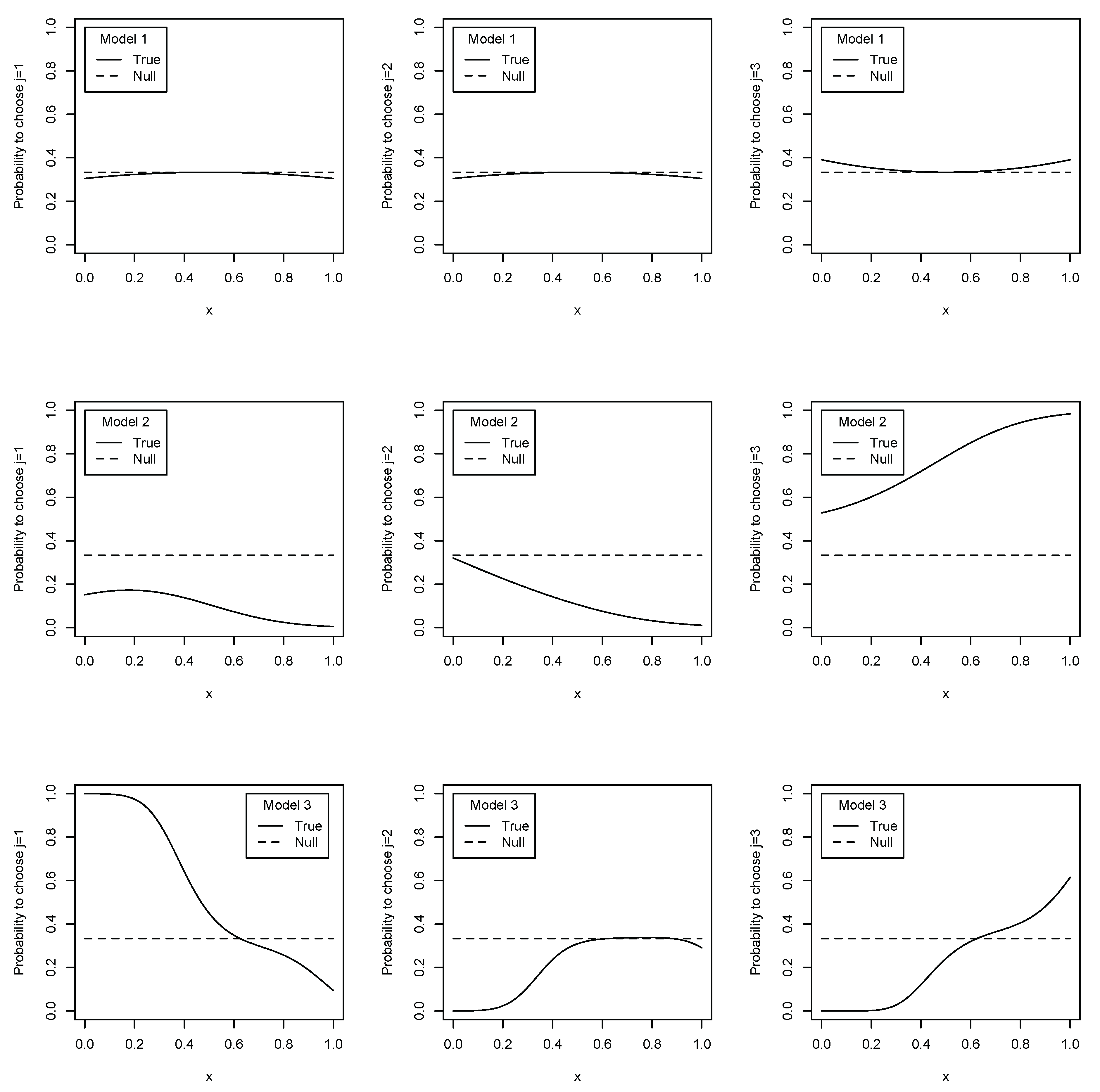
Before beginning to show the simulation results of the power performance of the test statistics, we illustrate the discrepancy between the true and parametric null models. The response probabilities in this simulation are mappings of the unit cube to the unit interval. For illustration simplicity, however, we focus on the domain of the response probabilities, being $\{X_i=(X_{i,1},X_{i,2},X_{i,3}):X_{i,j}\in [0,1]\text{for}\text{all}j\text{and}{X}_{i,1}=X_{i,2}=X_{i,3}\}$. In this setting, the fitted values for the response probabilities of the parametric model under the null hypothesis are always $1/3$ for all j, because the model does not have any alternative-variant coefficients.

Figure 1 shows how the true and null response probabilities react to the covariates. The larger distance between the true and null models with x fixed indicates that the parametric null model does not approximate the true model well. The parametric predictions of response probabilities lie closer to the true response probability in Model 1 than in Models 2 and 3 for all j. For the second and third alternatives, the parametric null response probability appears to lie closer to the true response probability in Model 3 than in Model 2. For the first alternative, however, the distance between the true and null models seems closer in Model 3. In brief, the null model gives the best response probability predictions in Model 1, but the predictions are less accurate in Models 2 and 3. The prediction precision of the null model could reflect the power performance of the test statistics.

Table 2 reports the proportion of rejections of the null hypothesis at the $5\%$ significance level. The first to third rows of the table show the power of the test when the true models are Model 1, Model 2 and Model 3, respectively, where the critical values are obtained by parametric bootstrap. Similarly, the fourth to sixth rows of the table show the power, where the critical values are obtained by the $95\%$ quantile of the chi-squared distribution with two degrees of freedom. The first to fourth columns of the table illustrate the power results obtained with a sample size of $n=50$ and bandwidths h of $0.30$, $0.35$, $0.40$ and $0.45$, respectively. Similarly, the fifth to eighth columns show the result with $n=100$.

The test does not have a decidedly nontrivial power when Model 1 is true. Non-rejection of the null hypothesis does not imply that the null model is true. However, in fact, as the top three figures in Figure 1 show, the parametric model under the null hypothesis may provide a proper approximation for the response probabilities of Model 1. Therefore, the low power of the test statistic may be acceptable. In contrast, the test statistic has more nontrivial power when Model 2 or 3 is true. The greater the sample size, the better the power performance, which depends on the choice of bandwidth.

Figure 1. Discrepancy between true and estimated parametric response probabilities.

Figure 1. Discrepancy between true and estimated parametric response probabilities.

Table 2. Proportion of null hypothesis rejections based on Monte Carlo simulation.

Critical Value	Model\h	$n=50$				$n=100$
		$0.30$	$0.35$	$0.40$	$0.45$	$0.30$	$0.35$	$0.40$	$0.45$
$t_{0.05}^{*}$	Model 1	$0.061$	$0.058$	$0.055$	$0.070$	$0.065$	$0.053$	$0.063$	$0.076$
	Model 2	$0.810$	$0.888$	$0.935$	$0.960$	$0.998$	$1.000$	$1.000$	$1.000$
	Model 3	$0.236$	$0.330$	$0.397$	$0.411$	$0.672$	$0.709$	$0.791$	$0.838$
$t_{0.05}$	Model 1	$0.047$	$0.043$	$0.056$	$0.061$	$0.049$	$0.053$	$0.052$	$0.053$
	Model 2	$0.807$	$0.907$	$0.940$	$0.970$	$0.995$	$1.000$	$0.999$	$1.000$
	Model 3	$0.255$	$0.304$	$0.365$	$0.415$	$0.600$	$0.713$	$0.777$	$0.839$

The significance level is $0.05$.

Table 2. Proportion of null hypothesis rejections based on Monte Carlo simulation.

Critical Value	Model\h	$n=50$				$n=100$
		$0.30$	$0.35$	$0.40$	$0.45$	$0.30$	$0.35$	$0.40$	$0.45$
$t_{0.05}^{*}$	Model 1	$0.061$	$0.058$	$0.055$	$0.070$	$0.065$	$0.053$	$0.063$	$0.076$
	Model 2	$0.810$	$0.888$	$0.935$	$0.960$	$0.998$	$1.000$	$1.000$	$1.000$
	Model 3	$0.236$	$0.330$	$0.397$	$0.411$	$0.672$	$0.709$	$0.791$	$0.838$
$t_{0.05}$	Model 1	$0.047$	$0.043$	$0.056$	$0.061$	$0.049$	$0.053$	$0.052$	$0.053$
	Model 2	$0.807$	$0.907$	$0.940$	$0.970$	$0.995$	$1.000$	$0.999$	$1.000$
	Model 3	$0.255$	$0.304$	$0.365$	$0.415$	$0.600$	$0.713$	$0.777$	$0.839$

The significance level is $0.05$.

Closer inspection of Table 2 reveals that the test performs better in terms of power when the critical values are obtained by parametric bootstrap, especially when the sample size is $n=50$. Too see this, we compare the results of $h=0.35$ when critical values are $t_{0.05}^{*}$ with those of $h=0.30$ when critical values are $t_{0.05}$. We compare the results with different bandwidths because the size of the test is close to its nominal size with these bandwidths ($0.047$ and $0.049$, respectively). When the true model is Model 2, the probability of the rejection of the null hypothesis is $0.888$ for $t_{0.05}^{*}$. The probability of the rejection is $0.807$ for $t_{0.05}$. Similarly, when the true model is Model 3, the probability is $0.330$ for $t_{0.05}^{*}$ and $0.255$ for $t_{0.05}$. It is surprising that the performance of the test is not unreasonable when critical values are obtained by an asymptotic distribution. However, at least in this setting, the test shows higher power when critical values are obtained by parametric bootstrap when the sample size is small.

7. Conclusions

This study proposes a consistent specification test for unordered multinomial choice models. It tests the specifications of multiple response probabilities jointly for all choice alternatives. The test statistic is asymptotically chi-square distributed with $J-1$ degrees of freedom, consistent against a fixed alternative and have nontrivial power against local alternatives approaching the null at the rate of $1/\sqrt{n{h}^{q/2}}$. The rejection region for the test statistic can be calculated through a simple parametric bootstrap procedure, when the sample size is small. In Monte Carlo experiments, we test the specification of the MNL model under three true models to examine the power performance of the test. We find that the test statistic does not have a decidedly nontrivial power when the parametric model under the null hypothesis provides a proper approximation for the response probabilities of the true model. The test statistic has more nontrivial power when the approximation of the null model is less successful. In addition, we find that the test shows higher power performance when critical values are obtained by parametric bootstrap than when they are obtained by the asymptotic distribution of the test statistic. The differences of the power performances are greater when the sample size is small. We can reduce size distortion by choosing an appropriate bandwidth, but this issue remains for future research.

The test proposed in this study can be applied to testing the parametric specifications of response probabilities for any unordered multinomial choice models, including the MNL and MNP models. However, the test is not able to detect local alternatives approaching the null hypothesis at the parametric rate, nor is it rate-optimal. Extending the testing procedure to incorporate such features is left for future research.

References

1. D. McFadden. “Conditional Logit Analysis of Qualitative Choice Behavior.” In Frontiers in Econometrics. Edited by P. Zarembka. New York, NY, USA: Academic Press, 1974, pp. 105–142. [Google Scholar]
2. J.A. Hausman, and D.A. Wise. “A Conditional Probit Model for Qualitative Choice: Discrete Decisions Recognizing Interdependence and Heterogeneous Preferences.” Econometrica 46 (1978): 403–426. [Google Scholar] [CrossRef]
3. S. Berry, J. Levinsohn, and A. Pakes. “Automobile Prices in Market Equilibrium.” Econometrica 63 (1995): 841–890. [Google Scholar] [CrossRef]
4. P.K. Goldberg. “Product Differentiation and Oligopoly in International Markets: The Case of the US Automobile Industry.” Econometrica 63 (1995): 891–951. [Google Scholar] [CrossRef]
5. J.J. Heckman. “The Common Structure of Statistical Models of Truncation, Sample Selection and Limited Dependent Variables and a Simple Estimator for Such Models.” Ann. Econ. Soc. Meas. 5 (1976): 475–492. [Google Scholar]
6. J.A. Dubin, and D.L. McFadden. “An Econometric Analysis of Residential Electric Appliance Holdings and Consumption.” Econometrica 52 (1984): 345–362. [Google Scholar] [CrossRef]
7. W. Härdle, and E. Mammen. “Comparing Nonparametric versus Parametric Regression Fits.” Ann. Stat. 21 (1993): 1926–1947. [Google Scholar] [CrossRef]
8. H.J. Bierens. “Consistent Model Specification Tests.” J. Econ. 20 (1982): 105–134. [Google Scholar] [CrossRef]
9. H.J. Bierens. “Model Specification Testing of Time Series Regressions.” J. Econom. 26 (1984): 323–353. [Google Scholar] [CrossRef]
10. H.J. Bierens. “A Consistent Conditional Moment Test of Functional Form.” Econometrica 58 (1990): 1443–1458. [Google Scholar] [CrossRef]
11. M.A. Delgado. “Testing the Equality of Nonparametric Regression Curves.” Stat. Probab. Lett. 17 (1993): 199–204. [Google Scholar] [CrossRef]
12. R.M. De Jong. “The Bierens Test under Data Dependence.” J. Econom. 72 (1996): 1–32. [Google Scholar] [CrossRef]
13. D.W. Andrews. “A Conditional Kolmogorov Test.” Econometrica 65 (1997): 1097–1128. [Google Scholar] [CrossRef]
14. H.J. Bierens, and W. Ploberger. “Asymptotic Theory of Integrated Conditional Moment Tests.” Econometrica 65 (1997): 1129–1151. [Google Scholar] [CrossRef]
15. W. Stute. “Nonparametric Model Checks for Regression.” Ann. Stat. 25 (1997): 613–641. [Google Scholar] [CrossRef]
16. M.B. Stinchcombe, and H. White. “Consistent Specification Testing with Nuisance Parameters Present Only under the Alternative.” Econom. Theory 14 (1998): 295–325. [Google Scholar] [CrossRef]
17. X. Chen, and Y. Fan. “Consistent Hypothesis Testing in Semiparametric and Nonparametric Models for Econometric Time Series.” J. Econom. 91 (1999): 373–401. [Google Scholar] [CrossRef]
18. Y.J. Whang. “Consistent Bootstrap Tests of Parametric Regression Functions.” J. Econom. 98 (2000): 27–46. [Google Scholar] [CrossRef]
19. R.L. Eubank, and C.H. Spiegelman. “Testing the Goodness of fit of a Linear Model via Nonparametric Regression Techniques.” J. Am. Stat. Assoc. 85 (1990): 387–392. [Google Scholar] [CrossRef]
20. S. Le Cessie, and J.C. van Houwelingen. “A Goodness-of-fit Test for Binary Regression Models, Based on Smoothing Methods.” Biometrics 47 (1991): 1267–1282. [Google Scholar] [CrossRef]
21. J.M. Wooldridge. “A Test for Functional Form Against Nonparametric Alternatives.” Econom. Theory 8 (1992): 452–475. [Google Scholar] [CrossRef]
22. A.J. Yatchew. “Nonparametric Regression Tests Based on an Infinite Dimensional Least Squares Procedure.” Econom. Theory 8 (1992): 435–451. [Google Scholar] [CrossRef]
23. P.L. Gozalo. “A Consistent Model Specification Test for Nonparametric Estimation of Regression Function Models.” Econom. Theory 9 (1993): 451–477. [Google Scholar] [CrossRef]
24. Y. Aït-Sahalia, P.J. Bickel, and T.M. Stoker. “Goodness-of-fit Tests for Kernel Regression with an Application to Option Implied Volatilities.” J. Econom. 105 (2001): 363–412. [Google Scholar] [CrossRef]
25. M.A. Delgado, and T. Stengos. “Semiparametric Specification Testing of non-Nested Econometric Models.” Rev. Econ. Stud. 61 (1994): 291–303. [Google Scholar] [CrossRef]
26. J.L. Horowitz, and W. Härdle. “Testing a Parametric Model Against a Semiparametric Alternative.” Econom. Theory 10 (1994): 821–848. [Google Scholar] [CrossRef]
27. Y. Hong, and H. White. “Consistent Specification Testing via Nonparametric Series Regression.” Econometrica 63 (1995): 1133–1159. [Google Scholar] [CrossRef]
28. Y. Fan, and Q. Li. “Consistent Model Specification Tests: Omitted Variables and Semiparametric Functional Forms.” Econometrica 64 (1996): 865–890. [Google Scholar] [CrossRef]
29. P. Lavergne, and Q.H. Vuong. “Nonparametric Selection of Regressors: The Nonnested Case.” Econometrica 64 (1996): 207–219. [Google Scholar] [CrossRef]
30. J.X. Zheng. “A Consistent Test of Functional Form via Nonparametric Estimation Techniques.” J. Econom. 75 (1996): 263–289. [Google Scholar] [CrossRef]
31. Q. Li, and S. Wang. “A Simple Consistent Bootstrap Test for a Parametric Regression Function.” J. Econom. 87 (1998): 145–165. [Google Scholar] [CrossRef]
32. P. Lavergne, and Q. Vuong. “Nonparametric Significance Testing.” Econom. Theory 16 (2000): 576–601. [Google Scholar] [CrossRef]
33. Y. Fan, and Q. Li. “Consistent Model Specification Tests.” Econom. Theory 16 (2000): 1016–1041. [Google Scholar] [CrossRef]
34. J. Mora, and A.I. Moro-Egido. “On Specification Testing of Ordered Discrete Choice Models.” J. Econom. 143 (2008): 191–205. [Google Scholar] [CrossRef]
35. J. Fan, and L.S. Huang. “Goodness-of-fit Tests for Parametric Regression Models.” J. Am. Stat. Assoc. 96 (2001): 640–652. [Google Scholar]
36. J.L. Horowitz, and V.G. Spokoiny. “An Adaptive, Rate-Optimal Test of a Parametric Mean-Regression Model Against a Nonparametric Alternative.” Econometrica 69 (2001): 599–631. [Google Scholar] [CrossRef]
37. V. Spokoiny. “Data-Driven Testing the fit of Linear Models.” Math. Methods Stat. 10 (2001): 465–497. [Google Scholar]
38. Y. Baraud, S. Huet, and B. Laurent. “Adaptive Tests of Linear Hypotheses by Model Selection.” Ann. Stat. 31 (2003): 225–251. [Google Scholar]
39. C.M. Zhang. “Adaptive Tests of Regression Functions via Multiscale Generalized Likelihood Ratios.” Can. J. Stat. 31 (2003): 151–171. [Google Scholar] [CrossRef]
40. E. Guerre, and P. Lavergne. “Data-Driven Rate-Optimal Specification Testing in Regression Models.” Ann. Stat. 33 (2005): 840–870. [Google Scholar]
41. W. Härdle, M. Müller, S. Sperlich, and A. Werwatz. Nonparametric and Semiparametric Models. Berlin Heidelberg, Germany: Springer, 2004, p. 92. [Google Scholar]
42. J.L. Powell, J.H. Stock, and T.M. Stoker. “Semiparametric Estimation of Index Coefficients.” Econometrica 57 (1989): 1403–1430. [Google Scholar] [CrossRef]
43. P. Hall. “Central Limit Theorem for Integrated Square Error of Multivariate Nonparametric Density Estimators.” J. Multivar. Anal. 14 (1984): 1–16. [Google Scholar] [CrossRef]
• 1.Rate optimal tests are proposed by [36,37,38,39,40,43], among others.
• 2.To be accurate, the MNL model consists of alternative-variant coefficients whose response probabilities are indicated by P ( Y j = 1 | X ) = exp ( X β j ) / [ 1 + j = 1 J exp ( X β j ) ] . However, the models represented by alternative-variant coefficients are able to transform into a model with alternative-invariant coefficients without loss of generality, which is sometimes called a conditional logit model. In this paper, we describe only a model with alternative-invariant coefficients.