Space-Time Variation and Spatial Differentiation of COVID-19 Confirmed Cases in Hubei Province Based on Extended GWR


1
School of Resource and Environmental Sciences, Wuhan University, Wuhan 430079, China
2
School of Resources and Environment Science and Engineering, Hubei University of Science and Technology, Xianning 437100, China
*
Author to whom correspondence should be addressed.
ISPRS Int. J. Geo-Inf. 2020, 9(9), 536; https://doi.org/10.3390/ijgi9090536
Submission received: 30 July 2020
/
Revised: 2 September 2020
/
Accepted: 3 September 2020
/
Published: 8 September 2020
Abstract
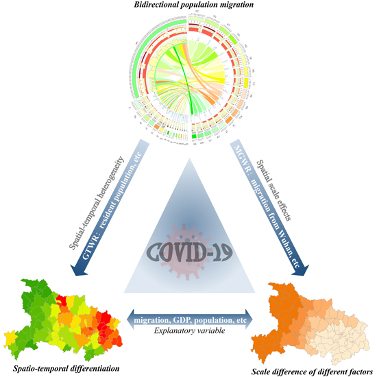
:Clarifying the regional transmission mechanism of COVID-19 has practical significance for effective protection. Taking 103 county-level regions of Hubei Province as an example, and taking the fastest-spreading stage of COVID-19, which lasted from 29 January 2020, to 29 February 2020, as the research period, we systematically analyzed the population migration, spatio-temporal variation pattern of COVID-19, with emphasis on the spatio-temporal differences and scale effects of related factors by using the daily sliding, time-ordered data analysis method, combined with extended geographically weighted regression (GWR). The results state that: Population migration plays a two-way role in COVID-19 variation. The emigrants’ and immigrants’ population of Wuhan city accounted for 3.70% and 73.05% of the total migrants’ population respectively; the restriction measures were not only effective in controlling the emigrants, but also effective in preventing immigrants. COVID-19 has significant spatial autocorrelation, and spatio-temporal differentiation has an effect on COVID-19. Different factors have different degrees of effect on COVID-19, and similar factors show different scale effects. Generally, the pattern of spatial differentiation is a transitional pattern of parallel bands from east to west, and also an epitaxial radiation pattern centered in the Wuhan 1 + 8 urban circle. This paper is helpful to understand the spatio-temporal evolution of COVID-19 in Hubei Province, so as to provide a reference for similar epidemic prevention.

1. Introduction
Viruses are potential threats to human survival. In December 2019, an atypical pneumonia named COVID-19, attributed to a novel corona virus of zoonotic origin, broke out in Wuhan, China [1]. It has been spreading boundlessly all over the world at an uncontrollable fast pace which people need to count the cases daily. Up until 24 July 2020, there have been 15,581,009 confirmed cases and 635,173 deaths in 216 countries [2]. The brutal epidemic has brought unprecedented pressure and challenge to the medical protection system of all countries in the world, and has had a serious impact on the current human business, economy, political relations and geospatial mobility. The effective containment of the epidemic is a top priority for governments and people from all walks of life. COVID-19 is neither the first nor last epidemic that we have been facing or are going to face. Therefore, it is of great practical importance to review the spatio-temporal variation and transmission mechanism of COVID-19 in the epicenter, Hubei Province, for the current and future epidemic prevention of similar viruses, when China’s domestic epidemic prevention has achieved periodic victory.
At the beginning of the COVID-19 outbreak, its rapid and large-scale spread in a short term made the primary task of the epidemic prevention to get timely information about the origin of virus, viral pathogenesis virus transmission, etc. [3]. A large number of scholars made timely insightful studies to find the characteristics of the virus itself and isolated the COVID-19 strains successfully, which laid a solid foundation for vaccine development. Since there is still much unknown knowledge about COVID-19 [4], some scholars have used multiple diffusion models such as dynamic model of infectious disease (SEIR), convLSTM to predict COVID-19 spread in advance [5,6,7], and some scholars have evaluated migration-to-immigration to virus relations and the potential risks in a post-epidemic era [8], in order to enhance the effectiveness of preventive measures. Scholars put much focus on the following factors when they used traditional Pearson’s statistic analytical approach [9], or when they introduced spatial auto-correlated spatial information models such as Moran’s I, LISA [10], or spatio-temporal information models concerning panel date [11], in order to find the related dominant factors of COVID-19 transmission. These are pathological factors directly related to patients themselves (their ages, whether or not they have other diseases, etc.) and factors associated with external environment (travel migration, population density, region GDP, traffic network, temperature and humidity, etc.). Spatial analysis tools and methods such as GIS and spatial statistics play an important role in the exploration process [12]. In view of the pathological characteristics of COVID-19, that it can be transmitted between people, some scholars have carried out studies targeted at the influence mechanism of population migration and transmission [13] and the effectiveness of government intervention measures [14,15], after the conventional factor-selection process. This research focused on different levels from the whole world, nations, provincial and municipal regions [16,17]. The county-level regions directed by the national policy were at the forefront of the epidemic prevention, but there were few studies focused on this level.
The COVID-19 outbreak has no regional stability but regional concentration, as in Hubei Province, with less than 2% of the territory, concentrated more than 80% of the patients [18]. Therefore, the epidemic has its specificity both in scale and transmission mechanisms. One of the problems emerging in the current studies on COVID-19 is that Hubei cases were often separated or excluded from the whole picture in previous studies’ analyses [5] because COVID-19 brought about a significantly higher risk of illness in Hubei Province than in the surrounding areas and there was significant difference between the severity of cases in Hubei province and those of cases from other provinces in China and other parts of the world [19]. Our research focused on the county scale to clarify the epidemic’s variation pattern in spreading and its spatial differentiation pattern. Therefore, it could provide a useful reference for effective protection when facing COVID-19 and other future similar viruses.
2. Materials and Methods
2.1. Overview of the Study Area
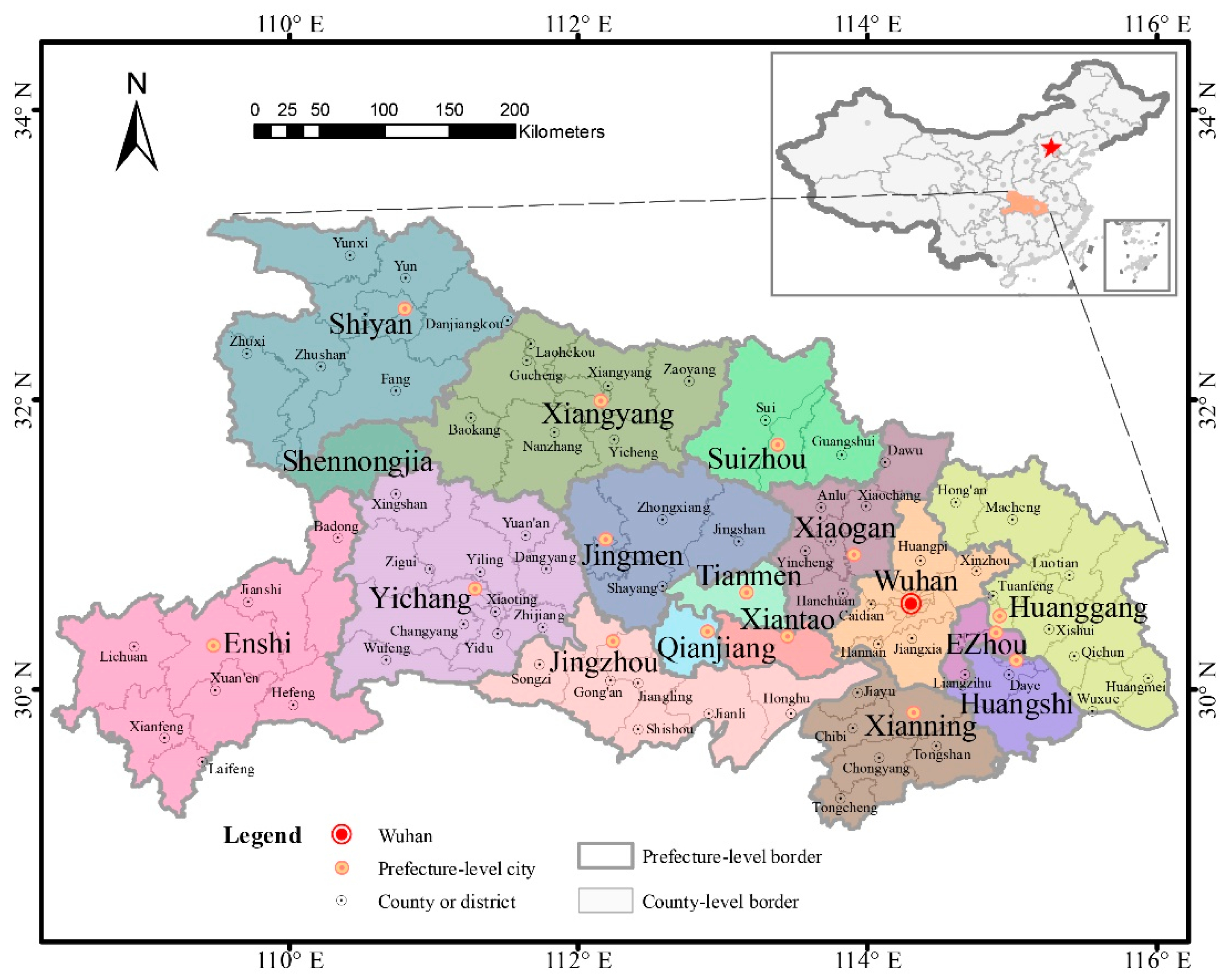
Hubei Province, located in central China (108°21′42″–116°07′50″E, 29°01′53″–33°6′47″N), has various and complex landform types and is surrounded by mountains in the east, west and north. In the middle of Hubei Province is the Jianghan Plain, which is a land of plenty. Hubei Province has an area of 185,900 square kilometers, accounting for 1.94% of the country’s territory and ranking as the 16th biggest province. The average annual temperature of Hubei Province is 15~18 °C. Its winter is cold and summer is hot. In this place, summer and winter are long, while spring and autumn are short. Rain and heat here come in the same season and its climate resources are rich and diverse. Though the precipitation is abundant, with an annual precipitation of 1201 mm, the distribution of the precipitation is not even at the levels of space and time. Hubei province is a transportation junction connecting east to west and south to north. Wuhan, the provincial capital famous for its links to various places since ancient times, is the center of the national high-speed railway network. Wuhan Tianhe International Airport is an important inland airport in China. Hubei Province has 1062 km of the Yangtze River running through it from west to east, passing Wuhan City. The airways, railways, highways and waterways all have tridimensional interchanges with each other. By the end of 2018, the resident population of Hubei Province has been 59.17 million, of which 11.081 million were in Wuhan. Hubei Province had a regional gross domestic product of 3936.655 billion yuan and a total of 987.1970 billion passengers of all kinds of traffic. The number of health institutions, health industry employees and beds was 36,397,521.8 thousand and 393.5 thousand respectively, with the beds’ utilization rate of 92.65% [20].
The spatial composition of administrative districts in Hubei Province includes 12 municipalities (Wuhan, Huangshi, Xiangfan, Jingzhou, Yichang, Shiyan, Xiaogan, Jingmen, Ezhou, Huanggang, Xianning and Suizhou), 1 autonomous prefecture (Enshi Tujia and Miao Ethnic Minority Autonomous Prefecture), 1 forest area (Shennongjia forest area) and 3 administrative units which are under the jurisdiction of Province (Xiantao, Qiangjiang, and Tianmen). In this paper, all 17 districts mentioned above are called city-level regions. These city-level regions can be divided into more elaborate districts or counties, which would be called county-level regions in the paper. The total number of these county-level regions is 103.
To more accurately understand the transmission mechanism of the COVID-19 and factors affecting its transmission, we took 103 county-level regions as the objects of the study. Some areas were re-zoned after examining the latest division of Hubei Province combined with the region in which the official information was published (Figure 1).
2.2. Data Sources
Provincial/prefecture-level/county-level geographic map data (2015) were obtained from the national basic geographic databases (the scale is 1:1 million), which were provided by the National Catalogue Service For Geographic Information (http://www.webmap.cn/). We made a few adjustments to correspond with the spatial scope of the publicly reported COVID-19 confirmed cases, since some administrative areas had been edited and updated according to the latest standard map (2020), which was downloaded from the website of Department of Natural Resources of Hubei Province (http://zrzyt.hubei.gov.cn/). All of the confirmed COVID-19 cases’ data were obtained from the latest bulletin of the official website. Among these, the epidemic data of three municipalities directly under the administration (Xiantao, Qiangjiang, and Tianmen) and one forest area (Shennongjia forest area) were obtained from Health Commission of Hubei Province. The data of the 13 districts in Wuhan City in the early stage were calculated based on the total cases in Wuhan in the early stage in proportion to a scale calculated by combining the partitioned statistical data in the later stage with the resident population, since there was no official partitioned statistical data in the early stage from Wuhan Municipal Health Commission. All the other county-level epidemic data were published on the official website of each municipal government or the website of the affiliated health committees. They were well organized according to the districts and counties, which were partitioned and administered by the cities. The data of railways, expressways, main roads and ordinary roads, etc., were obtained from Baidu Map (http://map.baidu.com/) and Amap (https://www.amap.com/), which were two public map service platforms. The 30-m-resolution impervious surfaces data of urban and rural from satellite remote sensing were downloaded from Finer Resolution Observation and Monitoring-Global Land Cover (http://data.ess.tsinghua.edu.cn/). Baidu migration index data (1 January 2020, to 29 February 2020) was obtained from Smarteye Map (https://qianxi.baidu.com/). The data of population, regional GDP in the county-level (districts, counties) in Hubei Province were obtained from the “Hubei Statistical Yearbook 2019 and 2018” and the Statistical Yearbook 2019 and 2018 of each prefecture-level city.
2.3. Research Methods
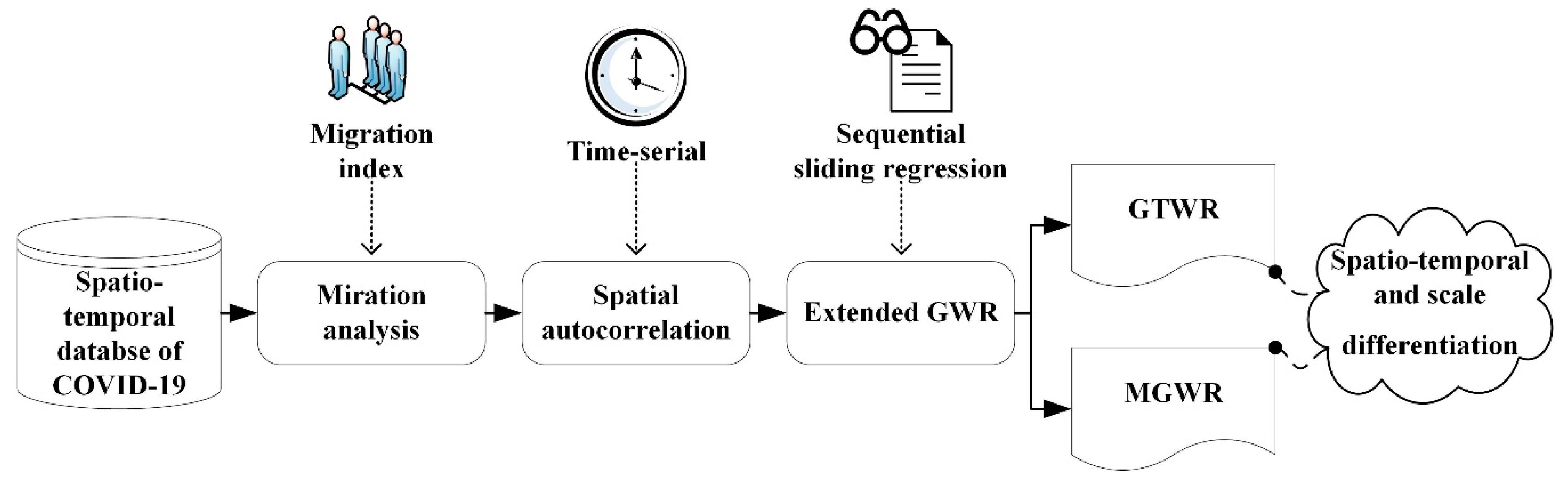
The general idea of the paper is shown in Figure 2. Firstly, the correlation between the migration and COVID-19 is analyzed by calculating the migration index. Secondly, the spatial autocorrelation of COVID-19 confirmed cases is explored by using time-serial data and Global Moran’s I. Finally, with the GTWR and MGWR of extended GWR models, the spatio-temporal and scale differentiation of COVID-19 confirmed cases are analyzed. In the analytical process, sliding analysis was carried out day by day for the time segments covering 32 days. Longer time segments were conducive to avoiding the occasional fluctuation, and sliding day by day was conducive to finding the optimal results due to the uncertain incubation period of COVID-19. The main methods are described below.
2.3.1. Geographically and Temporally Weighted Regression Model (GTWR)
The spread of COVID-19 epidemic in Hubei Province was not only different on the geographical level, but also different in time. Therefore, the rapid change in epidemic situation on a daily basis made the time factors especially important in model analysis, although the geographically weighted regression model (GWR) has the advantage that it extends the traditional regression analysis model by introducing location parameter, so that spatial heterogeneity can be reflected in the COVID-19 analysis, making the analysis results more reasonable. The GTWR model takes both time and spatial heterogeneity into account, and obtains the regression coefficients on each observation point by calculating the space–time distance, making the model theoretically closer to the reality. The GTWR model can be expressed as Formula (1) and the process of parameter-solving is in reference [21].
In this formula, i represents the ith observation (1 ≤ i ≤ n, n is the number of observations); k represents the kth independent variable, such as migration, GDP, population density, etc. (1 ≤ k ≤ m, m is the number of independent variables); Xik is the value of the kth independent variable at the ith observation point; εi represents the residual of the ith observation point; (μi,νi,ti) denotes the coordinates of the point i in spatio-temporal coordinate system; β0(μi,νi,ti) represents the intercept value, and βk(μi,νi,ti) is a set of values of parameters at points i, and it can change corresponding to time and space, which provides a more precise expression of the local effects.
In the GTWR local regression, the calculations of the adjacent points around the observation points depend on the spatial distance and temporal distance. Comprehensive results are obtained by adding operation. To balance the different effects of the methods used to measure the spatial and temporal distance in their respective metric systems, we gave out the spatial distance coefficient and the temporal distance coefficient (Formula 2), respectively. After the appropriate distance coefficient was given, the proximity degree could be measured.
In Formula (2), dST represents the spatial and temporal distance; dS and λ represent the spatial distance and coefficient, respectively; dT and μ represent the temporal distance and coefficient, respectively. If dT is smaller than dS, then it indicates that dST will be dominated by dS; if dT is bigger than dS, then it indicates that dST will be dominated by dT. In order to simplify the model, we defined k = μ/λ and λ = 1 in the actual operations. μ was optimized using cross-validation in terms of R2 or AIC [21].
2.3.2. Multi-Scale Geographically Weighted Regression (MGWR)
Tobler’s first law of geography lays a theoretical foundation for spatial autocorrelation analysis. The spatial range is a typical scale representation for GIS analysis [22]. In GWR, the heterogeneity of all spatial relationships at the same scale is captured by spatial bandwidth, but limiting the same spatial scale for all spatial processes may deviate the estimation results. For example, the temperature may vary little spatially, while the distances between the main roads depend on regional road density, which have obvious differences. MGWR, taking the different spatial scales that may exist between different independent variables into consideration, could allow conditional relationships between independent variables and dependent variables to change on different spatial scales [23] and different independent variables have expressions of different bandwidths in regression results. The following is the MGWR model [24].
In Formula 3, i represents the ith observation (1 ≤ i ≤ n, n is the number of observations); j represents the jth independent variable, such as migration, GDP, population density, etc.; m is the number of independent variables; xij is the value of the jth independent variable at the ith observation point; εi represents the residual of the ith observation point; (μi,νi) denotes the coordinates of the point i in space; bwj in βbwj indicates the bandwidth used for calibration of the jth conditional relationship; βbwj(μi,νi) is a set of values of parameters at points i. The process of parameter solving is in [24].
The bandwidth of the Extended GWR determines the rate at which regression weights attenuate in a given point’s ((u, v, t)/(u, v)) surrounding. The optimal bandwidth is determined by the AICc method [21]. The spatial kernel type is set to be adaptive.
2.3.3. Panel Data Sliding Regression
As our knowledge of COVID-19 is not complete, the result would be deviated from if we only use data from specific regions or at specific moments. However, panel data can provide individuals’ information about the dynamic behavior of individuals. Using cross-section and time, these two dimensions significantly increase the sample size, which can significantly improve the accuracy of the estimated results. According to the previous research, population migration is an important factor affecting the COVID-19 epidemic situation. Therefore, in this research, we collected data on the daily migration of population (the proportion of each city ‘s immigrants every day and the scale index of each city’s daily migration) in 17 city-level regions of Hubei province from 1 January 2020, to 29 February 2020. Considering the custom near the Spring Festival in domestic (that most migrations were for spending the Spring Festival in their hometowns) and the availability of the counties’ immigrant data, we proportioned the cities’ daily immigrant data onto 103 research districts based on every counties’ household registration population. In order to examine Wuhan emigrants’ effect on other districts, we sorted the migration data into two sections; one is on immigrants from Wuhan (Formula (4)) and the other is on immigrants from other regions (Formula (5)).
In these formulas, represents the immigratory index from Wuhan, while represents the immigratory index from other regions; i represents the ith county-level area (1 ≤ i ≤ 103); t represents the day from 1 January 2020 to 29 February 2020; ρit represents the immigrants’ percentage of the time t in area; represents the emigrant scale from Wuhan in t time; Ckt represents the emigrant scale from the kth area of the remaining 16 prefecture-level cities; the scale of emigrants among different prefectural cities in the same day is comparable.
According to the relatively complete official data on COVID-19 since 29 January 2020, the spread trend of the COVID-19 epidemic in Hubei Province in February 2020 was the most obvious. Until 29 February 2020, 85 of 103 county-level cities (82.52%) in the province already had zero newly confirmed cases. In order not to introduce more deviations into the later analyses, we only collected confirmed cases in the county-level from 29 January 2020 to 29 February 2020 in this paper.
The uncertainty of COVID-19′s incubation period made it difficult to accurately figure out the relationship between immigration data and confirmed cases. For example, the early-stage studies showed that the mean incubation period was 5.2 days (95% confidence interval [CI], 4.1 to 7.7.0) [25]. Tanu Singhal calculated the incubation period ranges from 2 to 14 d [26]. Patients who seem normal in the 14-day medical or isolated observation period and patients in the periods from pathogeny to diagnosis can all be potential source of infection. The uncertainty of COVID-19′s incubation period made it difficult to accurately figure out the corresponding relationship between the initial time of the immigration data and confirmed cases in the panel regression. In our analyses, we slid from day to day on the data of the immigrant factor to search for the optimal results. The sliding analyses’ method is in Formulas (6)–(8).
In these formulas, yi is a vector consisting of yi1, yi2,…, yi32 (shape is 1 × 32); and refer to the population migration vector from Wuhan and other regions, respectively, to the ith research area from day t. Since the incubation period of COVID-19 could not be precisely anticipated, the t value starts from 1 January 2020, and will then move on to every single day after that. Every time, population migration data for 32 consecutive days were taken for analysis. After 23 January 2020, due to the government’s strong travel intervention policy, the possibility of transmission caused by population migration was reduced sharply. In order not to let the data after the blocking of population migration have a too-large proportion in a single 32-day sequence analysis, the maximum value of the t was 29 January 2020. f was the statistical analysis method used in our study. Typical methods are GTWR and MGWR, which can be seen in references [9,10,27]. xpop、xGDP、xden were the resident population of each county-level units in 2018, GDP in the year 2018 and the population density of the area, respectively.
To explore the relationship between the change in human settlement environment and COVID-19, we introduced the impervious area variables ximp in various regions from 1978 to 2017 [28]. Levels of roads are the direct embodiment of traffic convenience; the completion of road infrastructure is directly related to the efficiency of population migration, and the carrying capacity of roads of different levels is not the same in population migration. In our study, the distances from each county-level district’s central point to railways, highways, main roads, secondary roads, other roads and subways were calculated, respectively. Since the subways are only in Wuhan City, we used their real distances in Wuhan City, while defined its value in other districts as 26,594 m, which is the same as the nearest district (Xiaogan). This means that subways have the same effect on the other districts. Entropy weight method was used to calculate the weights of all kinds of distance (Table 1), and then the sum of distances’ weights of all regions (xdis) was obtained as the final influence of the distances.
2.4. The Evolution of Population Migration between Prefecture-Level Cities
The reality that COVID-19 is infectious between people reveals that population migration is a non-negligible factor in the prevention and control of the epidemic’s spread [29,30]. We collected the immigrant population data between pairs of cities among the 17 prefecture-level cities of Hubei Province from 1 January to 29 February 2020. We drew circle maps using Circos to express the trend of migration, because it was not obvious after the restriction on travel was implemented. The timespan of the research was from 1 January 2020 to 31 January 2020 [31] (Figure 3).
On the right side of the Figure 3, the source of population migration is shown. We judged that the total amount of emigrants in each of the 17 cities in Hubei Province during 31 days in January was relatively balanced, while the destinations of the population have a significant trend of concentration. According to Table 2, the average population of the other 16 cities moving into Wuhan City is 73.05% when excluding the mutual migration within Wuhan City (Xiaogan has the maximum of 92.20%, while Shennongjia has the minimum of 43.64%). According to the migration destinations on the left side of Figure 3, Wuhan is very prominent in 17 prefectural-level cities. A total of 71.59% of the total migration population of Hubei Province in January 2020 moved to Wuhan, while the population of Wuhan City moving into other regions of the province only accounts for 3.70%. Wuhan is the economic and political center of Hubei Province. Its radiation effect on the surrounding areas is partly realized by the mobile workers whose families and companies are in Wuhan, while they are always or temporarily on business in other regions of the province. The beginning of the COVID-19 outbreak was coincidently close to the Spring Festival. This is the largest traditional festival in China, so many workers outside show an obvious trend of going back to their hometowns. The population’s trend of moving into Wuhan, mentioned above, exactly indicates this.
The migration data mainly decrease as the distance become longer. Wuhan is the migration center in the east of the province. Xiaogan, Ezhou, Xianning, Huanggang and Xiantao rank as the first five sources of the immigrants of Wuhan. The number of immigrants from Enshi is the lowest, only 21.93% of the amount of Xiaogan, which ranks the first. As for the emigrants of Wuhan, they mostly moved into Huanggang, Xiaogan, Jingzou, Xianning and Xiangyang, which rank as the first five destinations. The number of people moving into Huanggang is 6.19 times those into Xiangyang. In the western part of the province, migration circles which appear among cities near each other center on Shennongjia, Qianjiang, Enshi and Yichang. For example, the number of people moving from Shennongjia to Yichang and Xiangyang is, respectively, 13.27 and 4.32 times higher than that from Wuhan. The trend of immigration is the same as the urbanization degree of the regions, so emigrants to Shennongjia from each city account for the smallest population.
2.5. Time-Serial Spatial Autocorrelation of COVID-19
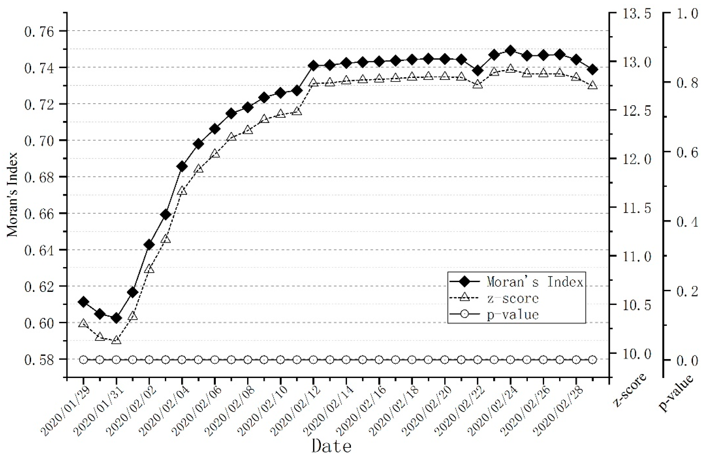
Since the early 1800s, scholars had identified a distance decay effect [32]. There is spatial interaction between the geographic data of one place and its adjacent location in the evolution of the COVID-19 spread. Moran’s I is often used to quantitatively describe the spatial autocorrelation of COVID-19 [33]. Using Global Moran’s I to analyze the COVID-19 confirmed cases of 103 research areas from 1 January 2020 to 29 February 2020, it can reveal the overall distribution of its spatial autocorrelation, which is helpful in quantitatively judging whether COVID-19 agglomeration occurs in space (Figure 4).
Figure 4 demonstrates that COVID-19 confirmed cases in the counties in Hubei Province have significant spatial autocorrelation from 1 January 2020 to 29 February 2020, which is basically consistent with some research results in reference [8]. The correlation degree tends to be stable after rapid growth in the early stage, which can generally be divided into four stages. The first is the decline phase (29 January 2020 to 31 January 2020) when Hubei Province implemented the severest population isolation policy and restriction on travel because of the rapid spread of the epidemic [1]. This led to the effective control of the fast-spread trend of the epidemic in the early stage. The second stage is the rapid growth period (1 February 2020 to 11 February 2020). In this stage, the incubation period of the virus-carrying population gradually ended and the disease gradually emerged after the policy of isolation and restriction. In the meantime, the new fast-detection technology, such as isothermal amplification kit, enhanced the detection ability per unit time. Therefore, a variety of factors resulted in a concentrated outbreak of the COVID-19 confirmed cases and the global spatial autocorrelation increased significantly. The third period is the smooth transition period (12 February 2020 to 23 February 2020). In this period, all the medical and public health teams and medical supplies from other provinces gathered to help out in every districts of Hubei Province. New hospitals for infectious diseases and mobile compartment hospitals were put into use. Isolation measures in the level of communities were strengthened [34]. All these factors contributed to the effective containment of the rapid growth trend of the COVID-19 epidemic. The cumulative number of cases in each county changed slightly, so the time-series spatial autocorrelation curve tends to be steady (the fluctuation on 12 February 2020 and 23 February 2020 are caused by the change in statistical caliber). The fourth period (24 February 2020 to 29 February 2020). In this stage, the comprehensive effect of various epidemic prevention measures had gradually emerged. The confirmed cases in other counties except Wuhan were dominated by stopping the increase. With the continuous increase in cured cases, the COVID-19 confirmed cases will be fewer and fewer, and the time-series spatial autocorrelation curve at the end of this stage showed a downward trend.
2.6. The Results of Extended GWR Sequential Sliding Regression
Spatio-temporal correlation and spatio-temporal heterogeneity are two significant features of spatio-temporal data [35]. Not only will the heterogeneity of spatial effect affect the spread of COVID-19, but the complex temporal effect will lead to the non-stationarity of COVID-19 confirmed cases’ evolution. Figure 5 shows the results of sequential sliding regression under different spatiotemporal patterns. The summaries of the OLS, GTWR and MGWR models are shown in Table 3.
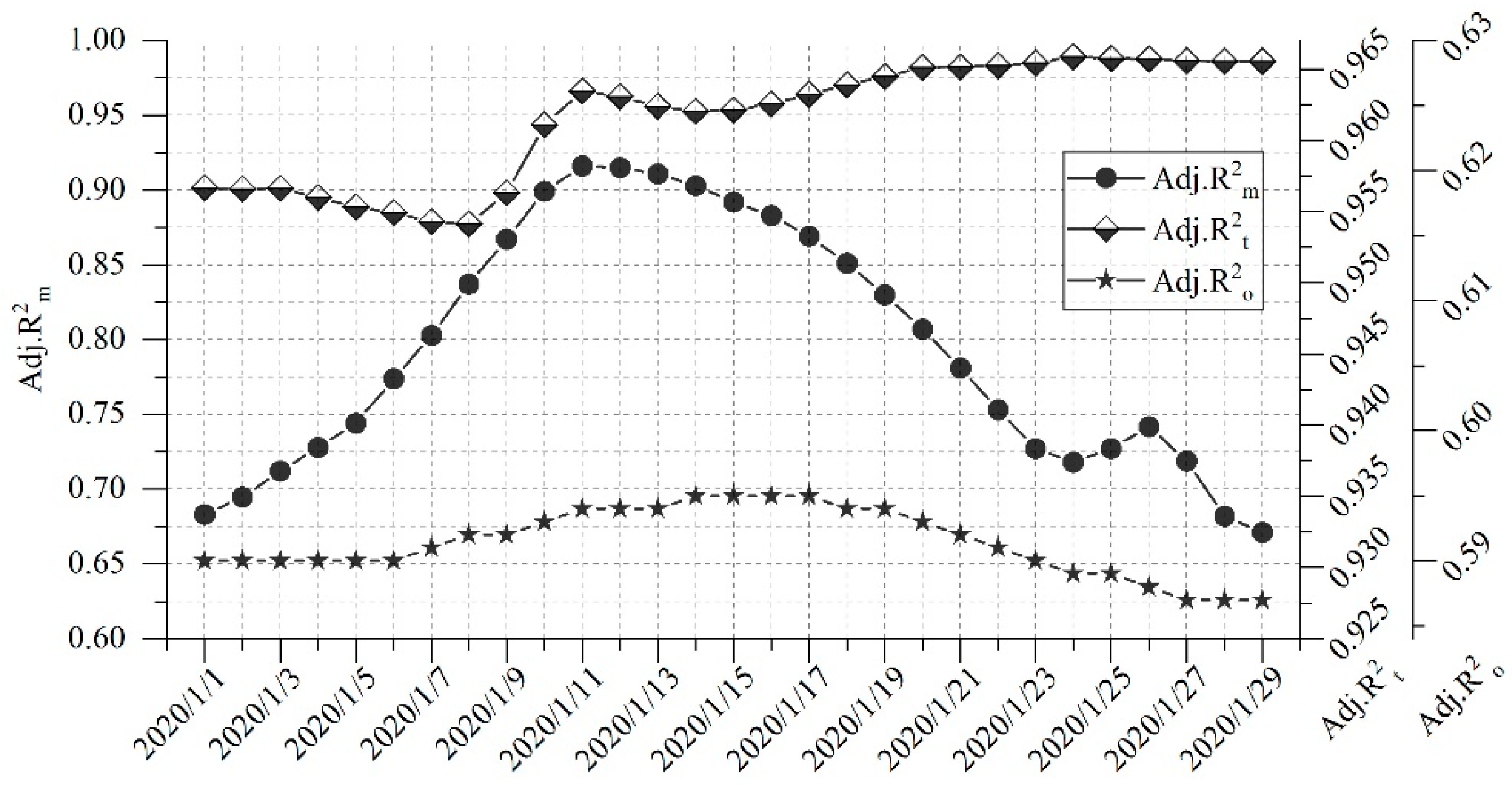
From Figure 5, we can see that OLS had the best regression result from 14 January 2020 to 17 January 2020. This implies that when it comes to COVID-19 confirmed cases in the 103 county-level regions in Hubei Province on the whole (1 January 2020 to 29 February 2020), the regression obtained the optimal results after 12–15 days of population migration when considering the influencing factors of population migration. The maximum of the adjusted R2 is 0.596. In GTWR regression, after considering the spatial and temporal heterogeneity, the adjusted R2 after the sequence regression from 1 January 2020 to 8 January 2020 decreased steadily in general. From 8 January 2020 to 11 January 2020, the adjusted R2 increased fast and the peak value appearing at the last day was 0.963. From 11 January 2020 to 24 January 2020, it decreased slightly and then increased slowly, and reached the overall maximum value of 0.966 at 24 January 2020. After that, due to the all-district severe restriction on travelling from 23 January 2020 and other factors, the adjusted R2 had an overall slow decline from 0.966 to 0.965 from 24 January 2020 to 31 January 2020. The Spatio-Temporal Distance Ratio increased from 0.269 to 0.373 (5 January 2020 to 8 January 2020) and then dropped back to 0.269. This demonstrates that spatial heterogeneity is dominant in spatiotemporal heterogeneity, and temporal heterogeneity fluctuates. MGWR regression, on the basis of spatial heterogeneity, takes spatial scale differences of different variables into consideration. In MGWR sequential sliding results, the adjusted R2 shows a fast climbing trend from 1 January 2020 to 11 January 2020, indicating that the effect of variable scale effect on regression results is enhanced. For example, the spatial scale of Intercept, xWH, xOther, xpop, xGDP, xdis, xden and ximp on 5 January 2020 is 68, 3270, 394, 431, 3270, 137, 68 and 1034, respectively, which is different from GWR, in which all the variables have the same spatial scale. MGWR have optimal regression results on 11 January 2020, at which point the adjusted R2 is 0.916. After that, the downward trend of the adjusted R2 of MGWR regression curve is obvious. Although it fluctuates slightly after 23 January 2020 when the restriction was implemented, the overall trend is still downward.
3. Discussion
3.1. Bidirectional Population Migration
For specific areas, population migration can be divided into two types: emigration and immigration. Assuming that transmission between humans is one of the main transmission routes of COVID-19, its influence pattern is bidirectional. Firstly, the corona virus carriers have a positive effect on the patient population of their destination. Some scholars’ studies on confirmed cases in destinations of Wuhan migration population showed that there is a significant positive correlation between them [36], and the destinations were mainly outside the epicenter, Hubei province (the amount of confirmed cases in and outside the province have a significant difference). Secondly, the migration of the healthy population has a dilution effect on the patient density of the destinations. Wuhan is a city with a population of tens of millions. Before the lockdown of the city, COVID-19 confirmed cases accounted for a very low population, so the density was also low [37] (on 23 January 2020, it was officially announced that 549 people were cumulative infections [1]). In addition, it was near the Spring Festival, so the population migration in the province mainly returned to Wuhan. Therefore, the prediction of the spread of COVID-19 confirmed cases based on large-scale population migration statistics such as mobile phone signaling has limited precision. However, the strict supervision of COVID-19 confirmed patients’ migration trajectory is more efficient and accurate. In the later stage, the reports on immigration at home and abroad were all concentrated on whether specific cases had a Wuhan travel history and there were few predictive reports based directly on migration data.
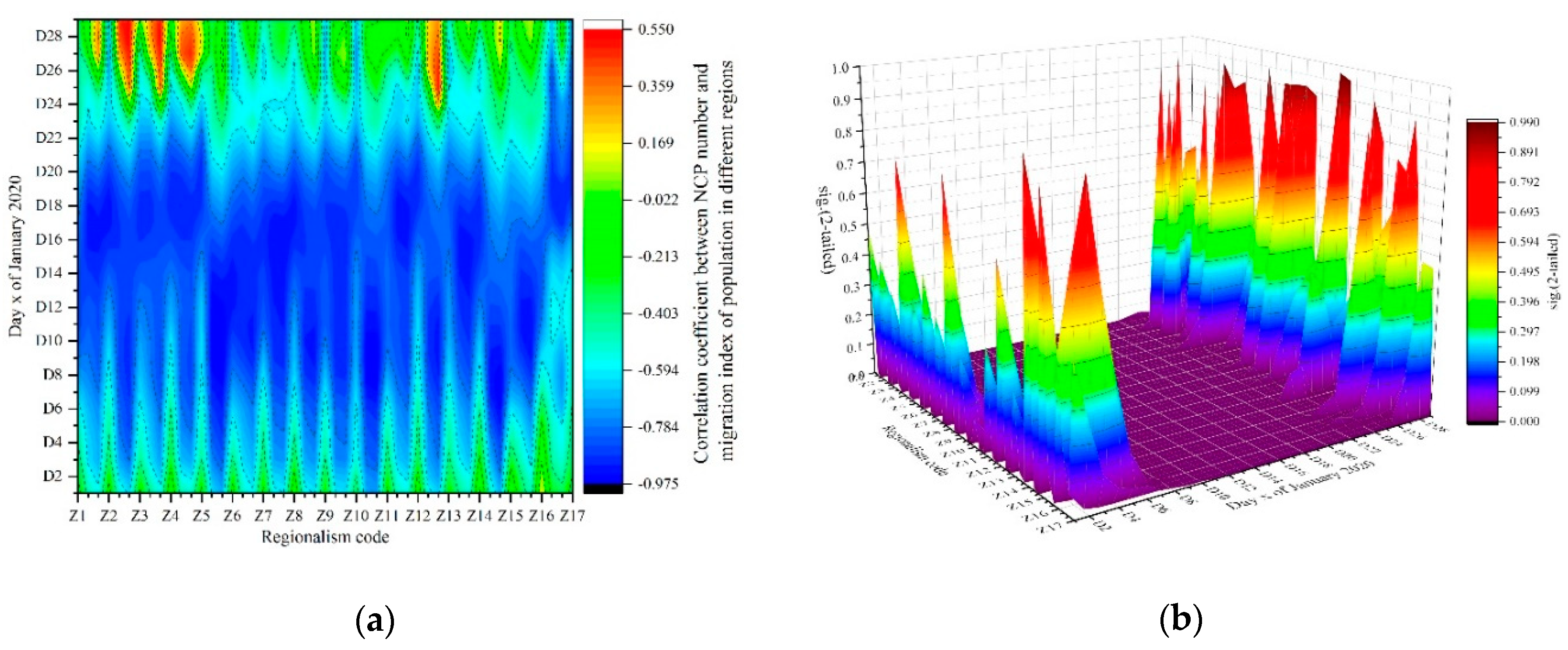
The period between 1 January 2020 and 29 February 2020 was the most typical stage of the COVID-19 concentrated outbreak in Hubei Province. The number of cases had rapid growth at the beginning of the month, while there were no new cases in most areas by the end of the month. The uncertainty of COVID-19′s incubation period made it difficult to accurately figure out the relationship between migration and COVID-19 confirmed cases. We take COVID-19 confirmed cases as the variable being explained and take the other 16 regions’ immigrant index as the variable used to explain from the mentioned 32-day cycle and eliminate the influence of mutation value as far as possible. We calculated the correlation (double tail) between paired cities from the 17 prefecture-level cities in Hubei Province day by day since 1 January 2020. Figure 6 is the correlation result and the corresponding significance.
From Figure 6a,b, we can see that the correlation of all regions shows a trend suggesting that there is positive/negative correlation from the beginning of the month, to the significant negative in middle of the month and the insignificant positive and negative correlation in the end of the month. The maximum correlation value of each district concentrated in the period from 14 January 2020 to 18 January 2020 and the correlation significance concentrated in the period from 8 January 2020 to 22 January 2020. The negative correlation of the main part shows that the migration population of 17 city-level scales was mainly healthy. During this period, the migration mode is mainly that people immigrate into Wuhan, which increases the risk of individual infection in the later stage and the cardinal number of the overall patient. Therefore, the restriction implemented on 23 January 2020 is an effective control measure, not only to prevent the emigrants of Wuhan being the sources of infection but also to prevent the high risk of immigrants of Wuhan getting the disease.
3.2. Co-Effects of Spatial Heterogeneity and Temporal Heterogeneity on COVID-19
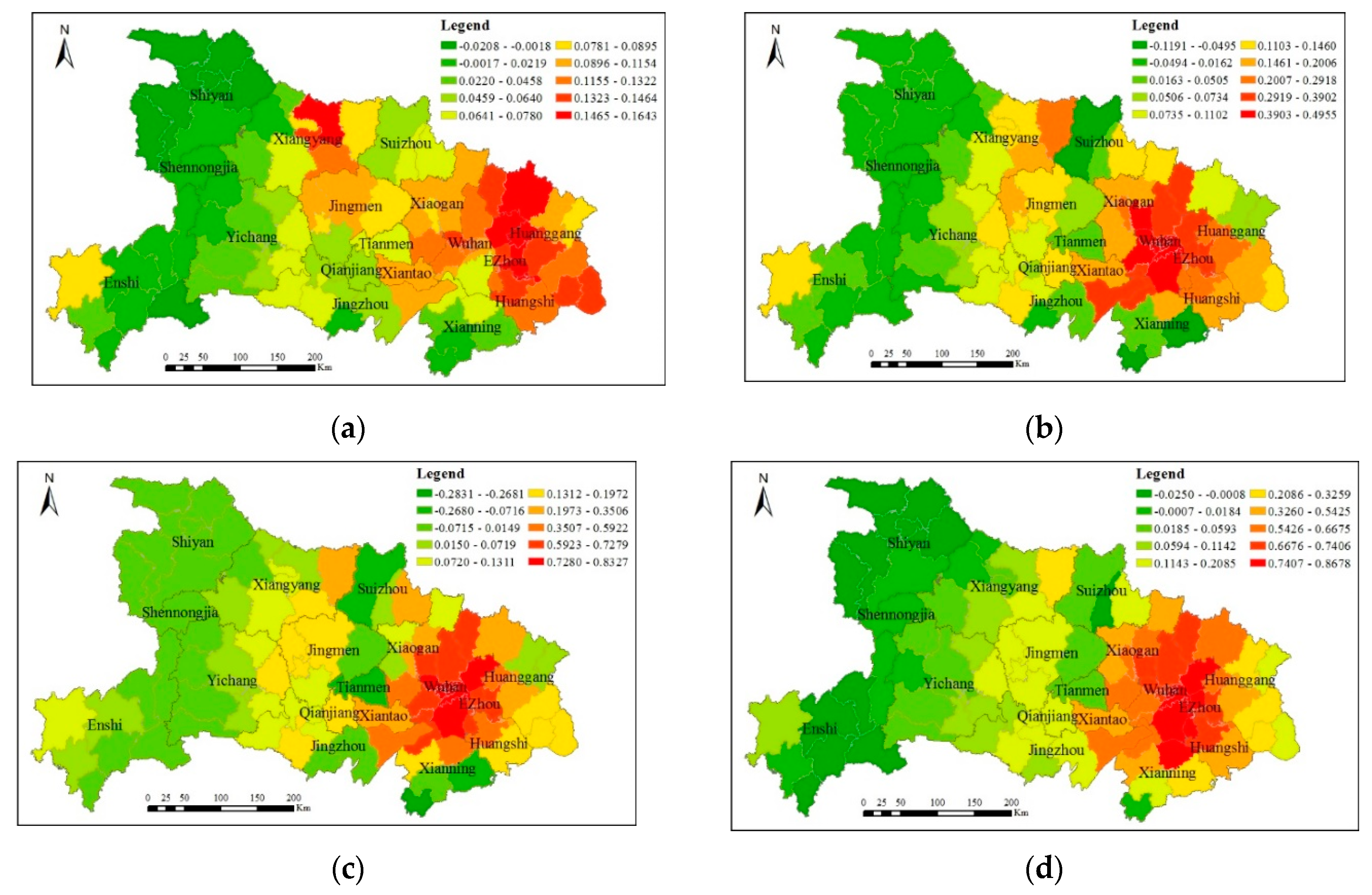
COVID-19′s evolution is closely related to environmental factors, mainly reflected in the two dimensions, which are space and time, respectively, based on the prior knowledge that anything has spatial correlation no matter whether it is strong or weak [38]. Differences in nature, humanities, etc., in different regions potentially affect COVID-19 development [9,39]. Referring to the spatial distance measurement method, the heterogeneity of the time dimension is reflected in the scale of the time-weighted element between observations i and j in the spatio-temporal weight matrix. Using 11 January 2020, when the adjusted R2 is optimal in the GWR time sequence sliding result, we divided the time range of 32 days into four stages and compared their spatio-temporal heterogeneities’ influence. It turned out that all the influencing factors were relatively clear in the first stage (11 January 2020 to 18 January 2020) and the second stage (19 January 2020 to 26 January 2020), while the third stage (27 January 2020 to 3 February 2020) and the fourth stage (4 February 2020 to 11 February 2020) were, relatively, a continuation of the second stage. Taking the resident population factor, which had a relatively big influence, as an example, the fourth stage changes are shown in Figure 7.
In Figure 7, we could see that the effect of resident population on COVID-19 has significant spatial-temporal differentiation. Taking Wuhan 1 + 8 city circle as the center, the influence degree gradually concentrates and shrinks from outside to inside. The Figure 7a shows that in the first stage when people could migrate freely, the impact of resident population on Xiangyang, Huanggang, Ezhou, Huangshi is the most significant. However, the overall impact is relatively extensive; its influence is obvious on cities near and far from Wuhan, such as Lichuan in western Hubei, Huangmei in eastern Hubei and Jingmen. Figure 7b shows that, with the implementation of the restriction on travel in Wuhan on 23 January 2020 and other areas of Hubei later, the center of the spatio-temporal influence of the resident population in the second stage gradually shrinks to the area centered on Wuhan. After the full implementation of the travel restriction, the spatial and temporal heterogeneity of the resident population no longer has great changes. Figure 7c,d presents that, in the third and fourth stages, the spatial and temporal differentiation is basically a continuation of the former stage. Wuhan 1 + 8 city circle concentrated about 52.83% of the province’s population and 60.35% of the GDP [40], and the trend of the spatial and temporal heterogeneity of the resident population centered in this circle became increasingly obvious.
3.3. The Spatial Scale Effects of Different Factors Vary
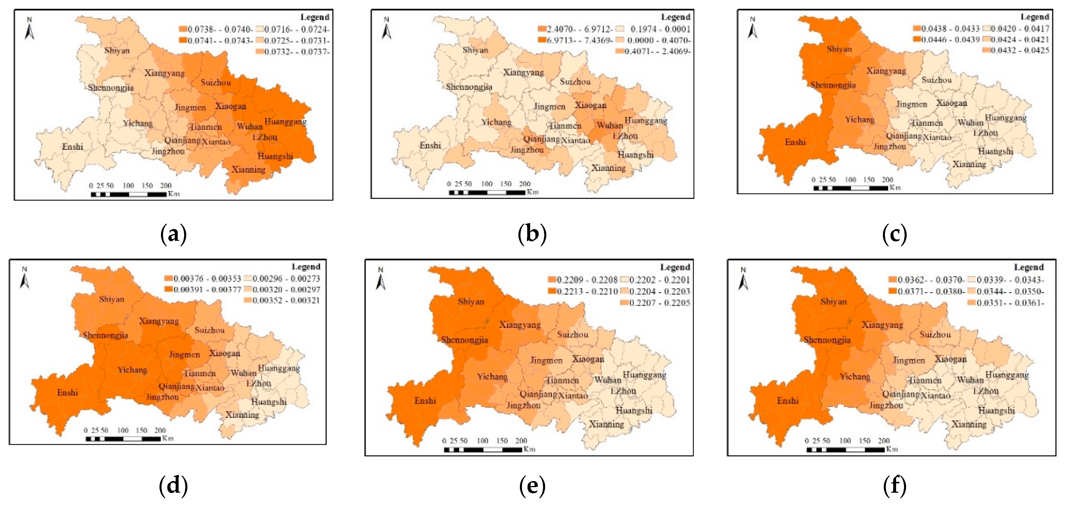
Resolution and extent are two typical scale representations in geographical analysis. Here, the scale means to extend. Ideally, models of physical process would be defined and tested on scale-free data [22], but classical GWR models give different factors the same spatial scale while considering spatial heterogeneity, which means that in COVID-19 evolution analysis, factors such as population density and distances to roads have the same spatial effective scope. However, it is obvious that the same road passing through areas with high-density population or areas with low-density population makes a difference on the spread of COVID-19. Figure 8 provides the scale difference of the other six factors on COVID-19 besides the population density factor which has been mentioned before.
From Figure 8, it could be seen that different factors have different degrees of influence on COVID-19, and factors of the same class show different scale effects. Figure 8a shows that immigrants from Wuhan had a more sensitive influence on the northeast of the province than on the southwest. The transition of the influence range is generally in the pattern of parallel band, and the gradation is very clear. The negative nature of the whole region indicates that within 32 consecutive days since 11 January 2020, the influence of immigrants from Wuhan had decreased due to the migration restriction on the 13th day in the period, and the decrease was more significant in the northeast. It is apparent from Figure 8b that the population migration of other regions has the most significant effect on Wuhan and the scale effect is the most obvious. The negative nature of the number indicates that under the condition that all the other factors were equal, the influence immigrants from other regions had on Wuhan COVID-19 situation was below the regional mean, while their influence on other regions like Enshi, Shennongjia, which are in the western Hubei Province and are far from Wuhan City, was above the regional mean. Figure 8c,e has a similar pattern of scale differentiation. The main part shows a level-by-level transition trend from big to small, from west to east. The ecological environment of the western part of the province is better than that of Wuhan and the eastern part, but the GDP and population density of the western part are far lower than that of the eastern part, so it is more sensitive to the change in GDP and population density. Figure 8d provides that the influence of traffic factors on Enshi, Yichang and other regions is relatively obvious. The geographical environment in this area is complex and diverse, so the traffic is less developed than that around Wuhan. Thus, the heterogeneity of all kinds of traffic is only apparent on a larger scale. Figure 8f implies that there is a negative relationship between the impervious surface and COVID-19. That means the larger the impervious area is, the better the habitat environment is, and the lower the number confirmed cases is. The impervious surface has a smaller impact on Wuhan, Ezhou and their surrounding areas, while it has a relatively big impact on regions like Enshi, Shennongjia and Shiyan. It is probably because impermeable surface construction in Wuhan and its surrounding reached a very high degree compared with the western area. Therefore, relatively speaking, the impact of the change in impermeable surface is less obvious than that in the west.
4. Conclusions
Migration has a bidirectional influence on the spread of COVID-19. The population from other regions in Hubei Province to Wuhan were mainly returning home to spend the Spring Festival before 23 January 2020, when the restrictions were implemented in Wuhan. The impact of the nearby migration in the western part of the province was obvious from 29 January 2020 to 29 February 2020 (slide day by day since 1 January 2020, and 32 days are a single period), the correlation between the accumulated COVID-19 confirmed cases of 103 county-level units in the whole province and the immigrant population showed an inverted U pattern, with a negative correlation in the early stage, and transitioned to a positive/negative correlation in the later stage. There was high significance from 8 January 2020 to 22 January 2020. The correlation maximum of each district appeared in a different time, with 16 January 2020 as the center, and concentrated in the period from 14 January 2020 to 18 January 2020. Potentially, it could be judged that the COVID-19 epidemic outbreak in February had the biggest relation with the population migration 11–15 days ahead of it. The negative correlation of each district’s correlation maximum shows that the effect of population immigration on destinations apart from Wuhan is still obvious, and effective epidemic prevention should not only focus on restricting the migration of the COVID-19 confirmed cases, but also take restriction measures to actively prevent cross-infection of healthy people who move into high-risk areas. As COVID-19 confirmed cases integrated in a dense flow of healthy people, it is an efficient protective way to isolate and restrict travel specifically in order to block the spread based on population migration. Similar population migration measures could be used for the prevention of other viruses or the same virus in other regions.
COVID-19 is significantly spatially auto-correlated. Its evolution in Hubei Province was both influenced by temporal differentiation and spatial differentiation, with the latter one as the main effect. The temporal differentiation is closely related with the population migration. Its influence has obvious stages. Before the travel restriction, the temporal differentiations of immigrant population vary obviously, while after the restriction, the spatio-temporal differences become steady. At each moment of the sliding regression, the adjusted R2 of GTWR is bigger than that of MGWR. The combined effect of spatial differentiation and temporal differentiation is more obvious than the variable scale effect. The evolution of COVID-19 has spatial concentration and temporal continuity, and timely prevention measures are of great significance to combat the further spread of the epidemic.
Different factors affect COVID-19 to different extent and factors of the same class show different variable scale effects. From the spatial aspect, the variable scale effect of COVID-19 confirmed cases in Hubei Province show a transition pattern of parallel bands from east to west and an epitaxial radiation pattern centered on the Wuhan 1 + 8 city circle. In the 32-day timespan, the resident population and population density have a great influence on the COVID-19 confirmed cases in the whole region, followed by factors including Wuhan’s immigration, regional GDPs and the impermeable surface. The traffic conditions have relatively little influence on the COVID-19 confirmed cases. As the Spring Festival approached, the immigration from other regions of Hubei Province had a relatively large influence on Wuhan and other regional economic centers. Therefore, we could conclude that the balanced development of the regions is beneficial to the reasonable migration of the population, thus alleviating the concentrated outbreaks of viruses.
Author Contributions
Zongyi He and Yanwen Liu conceived and designed the experiments, Yanwen Liu and Xia Zhou acquired and analyzed the data; Xia Zhou contributed analysis tools; Yanwen Liu prepared the original draft; Zongyi He and Xia Zhou reviewed and edited the manuscript; Others tasks were completed jointly by all the listed authors. All authors have read and agreed to the published version of the manuscript.
Funding
National Natural Science Foundation of China (No.41071290); Philosophy and Social Science Project of Hubei Province (No.19Q176).
Acknowledgments
The authors acknowledge the contribution of all the anonymous reviewers that improved the quality of the paper.
Conflicts of Interest
The authors declare no conflict of interest.
References
- Yang, Z.F.; Zeng, Z.Q.; Wang, K.; Wong, S.-S.; Liang, W.H.; Zanin, M.; Liu, P.; Cao, X.D.; Gao, Z.Q.; Mai, Z.T.; et al. Modified SEIR and AI prediction of the epidemics trend of COVID-19 in China under public health interventions. J. Thorac. Dis. 2020, 12, 165–174. [Google Scholar] [CrossRef] [PubMed]
- The Latest Statistic of the World Health Organization. 2020. Available online: https://www.who.int/COVID-19 (accessed on 25 July 2020).
- Yuen, K.S.; Ye, Z.W.; Fung, S.Y.; Chan, C.P.; Jin, D.Y. SARS-CoV-2 and COVID-19: The most important research questions. Cell Biosci. 2020, 10, 40. [Google Scholar] [CrossRef] [PubMed] [Green Version]
- Helmy, Y.A.; Fawzy, M.; Elaswad, A.; Sobieh, A.; Kenney, S.P.; Shehata, A.A. The COVID-19 pandemic: A comprehensive review of taxonomy, genetics, epidemiology, diagnosis, treatment, and control. J. Clin. Med. 2020, 9, 1225. [Google Scholar] [CrossRef] [PubMed]
- Chang, R.J.; Wang, H.W.; Zhang, S.X.; Wang, Z.Z.; Dong, Y.Q.; Tsamlag, L.; Yu, X.Y.; Xu, C.; Yu, Y.L.; Long, R.S.; et al. Phase- and epidemic region-adjusted estimation of the number of coronavirus disease 2019 cases in China. Front. Med. 2020, 14, 199–209. [Google Scholar] [CrossRef] [Green Version]
- Paul, S.K.; Jana, S.; Bhaumik, P. A multivariate spatiotemporal spread model of COVID-19 using ensemble of ConvLSTM networks. MedRxiv 2020. [Google Scholar] [CrossRef]
- Giuliani, D.; Dickson, M.M.; Espa, G.; Santi, F. Modelling and Predicting the Spatio-Temporal Spread of Coronavirus Disease 2019 (COVID-19) in Italy. 2020. Available online: https://ssrn.com/abstract=3559569 (accessed on 15 July 2020).
- Wang, Z.H.; Yao, M.Y.; Meng, C.G.; Claramunt, C. Risk assessment of the overseas imported COVID-19 of ocean-going ships based on AIS and infection data. ISPRS Int. J. Geo-Inf. 2020, 9, 351. [Google Scholar] [CrossRef]
- Xiong, Y.Z.; Wang, Y.P.; Chen, F.; Zhu, M.Y. Spatial statistics and influencing factors of the epidemic of novel coronavirus pneumonia 2019 in Hubei province, China. Res. Sq. 2020. [Google Scholar] [CrossRef] [Green Version]
- Cao, Z.D.; Wang, J.F.; Gao, Y.G.; Han, W.G.; Feng, X.L.; Zeng, G. Risk factors and autocorrelation characteristics on severe acute respiratory syndrome in Guangzhou. Dili Xuebao/Acta Geogr. Sinica 2008, 63, 981–993. [Google Scholar]
- Guliyev, H. Determining the spatial effects of COVID-19 using the spatial panel data model. Spat. Stat. 2020, 38, 100443. [Google Scholar] [CrossRef]
- Ivan, F.P.; Brian, M.N.; Fernando, R.V.; Lawal, B. Spatial analysis and GIS in the study of COVID-19. A review. Sci. Total Environ. 2020, 739, 140033. [Google Scholar] [CrossRef]
- Sirkeci, I.; Yucesahin, M.M. Coronavirus and migration: Analysis of human mobility and the spread of COVID-19. Migr. Lett. 2020, 17, 379–398. [Google Scholar] [CrossRef] [Green Version]
- Prem, K.; Liu, Y.; Russell, T.W.; Kucharski, A.J.; Eggo, R.M.; Davies, N.; Jit, M.; Klepac, P. The effect of control strategies to reduce social mixing on outcomes of the COVID-19 epidemic in Wuhan, China: A modelling study. Lancet Public Health 2020, 5, E261–E270. [Google Scholar] [CrossRef] [Green Version]
- Sebastiani, G.; Massa, M.; Riboli, E. Covid-19 epidemic in Italy: Evolution, projections and impact of government measures. Eur. J. Epidemiol. 2020, 35, 341–345. [Google Scholar] [CrossRef] [PubMed]
- Boulos, M.K.N.; Geraghty, E.M. Geographical tracking and mapping of coronavirus disease COVID-19/severe acute respiratory syndrome coronavirus 2 (SARS-CoV-2) epidemic and associated events around the world: How 21st century GIS technologies are supporting the global fight against outbreaks and epidemics. Int. J. Health Geogr. 2020, 19, 8. [Google Scholar] [CrossRef] [Green Version]
- Dorélien, A.M.; Ramen, A.; Swanson, I. Analyzing the Demographic, Spatial, and Temporal Factors Influencing Social Contact Patterns in US and Implications for Infectious Disease Spread. [Unpublished manuscript] Humphrey School of Public Affairs, University of Minnesota. Available online: http://www.audreydorelien.com/wp-content/uploads/2020/04/ATUS_social_contact_latest.pdf (accessed on 25 March 2020).
- The Latest Statistic of the National Health Commission of China. 2020. Available online: http://www.nhc.gov.cn (accessed on 15 July 2020).
- Tetro, J.A. Is COVID-19 receiving ADE from other coronaviruses? Microbes Infect. 2020, 22, 72–73. [Google Scholar] [CrossRef]
- Hubei Provincial Bureau of Statistics; Hubei Survey Team of National Bureau of Statistics. Hubei Statistical Yearbook; China Statistics Press: Beijing, China, 2019. [Google Scholar]
- Huang, B.; Wu, B.; Barry, M. Geographically and temporally weighted regression for modeling spatio-temporal variation in house prices. Int. J. Geogr. Inf. Sci. 2010, 24, 383–401. [Google Scholar] [CrossRef]
- Goodchild, M.F. Scale in GIS: An overview. Geomorphology 2011, 130, 5–9. [Google Scholar] [CrossRef]
- Yang, W.B. An Extension of Geographically Weighted Regression with Flexible Bandwidths. Ph.D. Thesis, University of St Andrews, St Andrews, UK, 2014. [Google Scholar]
- Fotheringham, A.S.; Yang, W.B.; Kang, W. Multiscale geographically weighted regression (MGWR). Ann. Am. Assoc. Geogr. 2017, 107, 1247–1265. [Google Scholar] [CrossRef]
- Li, Q.; Guan, X.H.; Wu, P.; Wang, X.Y.; Zhou, L.; Tong, Y.Q.; Ren, R.Q.; Leung, K.S.M.; Lau, E.H.Y.; Wong, J.Y.; et al. Early transmission dynamics in Wuhan, China, of novel coronavirus-infected pneumonia. N. Engl. J. Med. 2020, 382, 1199–1207. [Google Scholar] [CrossRef]
- Singhal, T. A review of coronavirus disease-2019 (COVID-19). Indian J. Pediatr. 2020, 87, 281–286. [Google Scholar] [CrossRef] [Green Version]
- Briz-Redón, Á.; Serrano-Aroca, Á. A spatio-temporal analysis for exploring the effect of temperature on COVID-19 early evolution in Spain. Sci. Total Environ. 2020, 728, 138811. [Google Scholar] [CrossRef] [PubMed]
- Gong, P.; Li, X.C.; Zhang, W.H. 40-Year (1978–2017) human settlement changes in China reflected by impervious surfaces from satellite remote sensing. Sci. Bull. 2019, 64, 756–763. [Google Scholar] [CrossRef] [Green Version]
- Mallapaty, S. Why does the coronavirus spread so easily between people? Nature 2020, 579, 183. [Google Scholar] [CrossRef] [PubMed] [Green Version]
- Jia, J.S.; Lu, X.; Yuan, Y.; Xu, G.; Jia, J.M.; Christakis, N.A. Population flow drives spatio-temporal distribution of COVID-19 in China. Nature 2020, 582, 389–394. [Google Scholar] [CrossRef] [PubMed]
- Krzywinski, M.; Schein, J.; Birol, I.; Connors, J.; Gascoyne, R.; Horsman, D.; Jones, S.J.; Marra, M.A. Circos: An information aesthetic for comparative genomics. Genome Res. 2009, 19, 1639–1645. [Google Scholar] [CrossRef] [PubMed] [Green Version]
- Getis, A. Reflections on spatial autocorrelation. Reg. Sci. Urban Econ. 2007, 37, 491–496. [Google Scholar] [CrossRef]
- Kang, D.; Choi, H.; Kim, J.H.; Choi, J. Spatial epidemic dynamics of the COVID-19 outbreak in China. Int. J. Infect. Dis. 2020, 94, 96–102. [Google Scholar] [CrossRef]
- Wang, H.W.; Wang, Z.Z.; Dong, Y.Q.; Chang, R.J.; Xu, C.; Yu, X.Y.; Zhang, S.X.; Tsamlag, L.; Shang, M.L.; Huang, J.Y.; et al. Phase-adjusted estimation of the number of coronavirus disease 2019 cases in Wuhan, China. Cell Discov. 2020, 6, 1–8. [Google Scholar] [CrossRef] [Green Version]
- Wang, H.X.; Wang, J.D.; Huang, B. Prediction for spatio-temporal models with autoregression in errors. J. Nonparametr. Stat. 2012, 24, 217–244. [Google Scholar] [CrossRef]
- Chen, Z.L.; Zhang, Q.; Lu, Y.; Guo, Z.M.; Zhang, X.; Zhang, W.J.; Guo, C.; Liao, C.H.; Li, Q.L.; Han, X.H.; et al. Distribution of the COVID-19 epidemic and correlation with population emigration from Wuhan, China. Chin. Med. J. 2020, 133, 1044–1050. [Google Scholar] [CrossRef]
- Peng, Z.H.; Wang, R.S.; Liu, L.B.; Wu, H.Z. Exploring urban spatial features of COVID-19 transmission in Wuhan based on social media data. ISPRS Int. J. Geo-Inf. 2020, 9. [Google Scholar] [CrossRef]
- Tobler, W. On the first law of geography: A reply. Ann. Assoc. Am. Geogr. 2004, 94, 304–310. [Google Scholar] [CrossRef]
- Sajadi, M.M.; Habibzadeh, P.; Vintzileos, A.; Shokouhi, S.; Miralles-Wilhelm, F.; Amoroso, A. Temperature and Latitude Analysis to Predict Potential Spread and Seasonality for COVID-19. SSRN. Available online: https://ssrn.com/abstract=3550308 (accessed on 5 March 2020).
- Li, H.; Liu, Y.L.; He, Q.S.; Peng, X.; Yin, C.H. Simulating urban cooperative expansion in a single-core metropolitan region based on improved CA model integrated information flow: Case study of Wuhan urban agglomeration in China. J. Urban Plan. Dev. 2018, 144, 05018002. [Google Scholar] [CrossRef]
Figure 1.
Sketch map of the research area.

Figure 2.
The flow chart of the analysis about COVID-19.

Figure 3.
Inter-population migration from 1 January 2020 to 31 January 2020. Note: (1) The capital letters and non-capital letters in the outer circles represent the cities people move out of and move into. (2) All scale labels represent the number of migrations in the corresponding area. (Multiply everything by 0.1 except the percentage and the innermost circle scale). (3) The scatter points are distributed at different levels; the line chart and the histogram show the sub-level composition of the migration information of each region. (4) The strips with different color and widths in the center of the circle diagram visually show the migration direction and quantity from move-out areas (Note those with capital letters in the outer circles, such as: EZ) to move-in areas (Note those with non-capital letters in the outer circles, such as: ez.).

Figure 4.
Time-serial spatial autocorrelation of COVID-19.

Figure 5.
Adjusted R2 time-serial sliding. Note: Adj. represents the adjusted R square after MGWR regression; Adj. represents the adjusted R square after GTWR regression; Adj. represents the adjusted R square after Global regression.
Figure 5.
Adjusted R2 time-serial sliding. Note: Adj. represents the adjusted R square after MGWR regression; Adj. represents the adjusted R square after GTWR regression; Adj. represents the adjusted R square after Global regression.

Figure 6.
Time-serial correlation between immigration and COVID-19 confirmed cases: (a) the correlation result; (b) the corresponding significance. Notes: D2 refers to the second day of January, 2020 and the labels can be explained similarly; Z1-Z17 refer to the 17 prefecture-level cities in Table 2; The different colors in Figure 6a, b reveal the degree of correlation at different spatio-temporal points and the significance of each corresponding point.

Figure 7.
The spatio-temporal differentiation of the resident population: (a) from 11 to 18 January 2020; (b) from 19 to 26 January 2020; (c) from 27 January to 3 February 2020; (d) from 4 to 11 February 2020.
Figure 7.
The spatio-temporal differentiation of the resident population: (a) from 11 to 18 January 2020; (b) from 19 to 26 January 2020; (c) from 27 January to 3 February 2020; (d) from 4 to 11 February 2020.

Figure 8.
The scale difference of different factors: (a) Migration form Wuhan; (b) Migration from other area; (c) GDP; (d) Integrated distance; (e) Population density; (f) Impervious areas.
Figure 8.
The scale difference of different factors: (a) Migration form Wuhan; (b) Migration from other area; (c) GDP; (d) Integrated distance; (e) Population density; (f) Impervious areas.


Table 1.
The weights of different roads.
| Road Type | Railway | Expressway | Main Road | Secondary Road | Other Road | Subway |
|---|---|---|---|---|---|---|
| Weight | 0.24 | 0.20 | 0.16 | 0.19 | 0.19 | 0.02 |
Table 2.
The migration index matrix for January 2020 in Hubei province.
| In Out | WH | HS | SY | YC | XY | EZ | JM | XG | JZ | HG | XN | SZ | ES | XT | QJ | TM | SN | Sum |
|---|---|---|---|---|---|---|---|---|---|---|---|---|---|---|---|---|---|---|
| WH | / | 97 | 30 | 67 | 104 | 93 | 52 | 529 | 239 | 644 | 133 | 38 | 41 | 32 | 9 | 19 | 0 | 2127 |
| HS | 2489 | / | 5 | 12 | 18 | 313 | 6 | 35 | 31 | 552 | 101 | 4 | 5 | 3 | 1 | 2 | 0 | 3577 |
| SY | 1642 | 14 | / | 33 | 518 | 4 | 21 | 40 | 51 | 40 | 9 | 15 | 8 | 3 | 2 | 3 | 1 | 2404 |
| YC | 1690 | 15 | 17 | / | 113 | 6 | 82 | 61 | 525 | 55 | 12 | 6 | 215 | 7 | 5 | 8 | 1 | 2818 |
| XY | 1874 | 14 | 159 | 74 | / | 6 | 69 | 60 | 69 | 41 | 11 | 57 | 10 | 3 | 2 | 4 | 0 | 2453 |
| EZ | 4391 | 709 | 4 | 10 | 15 | / | 6 | 40 | 31 | 401 | 36 | 4 | 4 | 3 | 1 | 2 | 0 | 5657 |
| JM | 2423 | 12 | 18 | 135 | 182 | 6 | / | 139 | 349 | 45 | 13 | 18 | 22 | 11 | 22 | 86 | 0 | 3481 |
| XG | 5056 | 15 | 11 | 27 | 48 | 9 | 35 | / | 56 | 101 | 19 | 53 | 6 | 21 | 2 | 25 | 0 | 5484 |
| JZ | 2088 | 10 | 8 | 179 | 31 | 5 | 59 | 61 | / | 34 | 28 | 4 | 20 | 35 | 32 | 9 | 0 | 2603 |
| HG | 3418 | 112 | 7 | 15 | 16 | 40 | 6 | 59 | 35 | / | 16 | 4 | 5 | 2 | 1 | 1 | 0 | 3737 |
| XN | 3461 | 98 | 6 | 17 | 19 | 17 | 8 | 56 | 102 | 71 | / | 4 | 6 | 6 | 1 | 3 | 0 | 3875 |
| SZ | 2843 | 13 | 25 | 23 | 266 | 8 | 31 | 372 | 51 | 52 | 13 | / | 6 | 3 | 1 | 4 | 0 | 3711 |
| ES | 1108 | 12 | 7 | 207 | 23 | 5 | 17 | 23 | 110 | 31 | 10 | 2 | / | 5 | 3 | 3 | 0 | 1566 |
| XT | 3144 | 11 | 8 | 35 | 25 | 5 | 25 | 260 | 431 | 42 | 18 | 4 | 13 | / | 49 | 106 | 0 | 4176 |
| QJ | 2080 | 10 | 10 | 50 | 24 | 4 | 115 | 97 | 933 | 44 | 11 | 4 | 14 | 120 | / | 49 | 0 | 3565 |
| TM | 1980 | 8 | 10 | 36 | 31 | 4 | 195 | 261 | 146 | 31 | 10 | 5 | 10 | 102 | 21 | / | 0 | 2850 |
| SN | 1513 | 8 | 194 | 889 | 449 | 3 | 34 | 50 | 110 | 10 | 6 | 7 | 179 | 6 | 5 | 4 | / | 3467 |
| sum | 41,200 | 1158 | 519 | 1809 | 1882 | 528 | 761 | 2143 | 3269 | 2194 | 446 | 229 | 564 | 362 | 157 | 328 | 2 | 57,551 |
1 WH for Wuhan, HS for Huangshi, SY for Shiyan, YC for Yichang, XY for Xiangyang, EZ for Ezhou, JM for Jingmen, XG for Xiaogan, JZ for Jingzhou, HG for Xianning, XN for Xianning, SZ for Suizhou, ES for Enshi, XT for Xiantao, QJ for Qianjiang, TM for Tianmen, and SN for Shennongjia.
Table 3.
Summaries of OLS, GTWR and MGWR models.
| Name | R2 | Adjusted R2 | AICc | |||||||||
|---|---|---|---|---|---|---|---|---|---|---|---|---|
| Max | Min | Median | Mean | Max | Min | Median | Mean | Max | Min | Median | Mean | |
| OLS | 0.596 | 0.588 | 0.592 | 0.592 | 0.595 | 0.587 | 0.591 | 0.592 | 6448.611 | 6387.235 | 6417.994 | 6413.252 |
| GTWR | 0.966 | 0.954 | 0.963 | 0.962 | 0.966 | 0.954 | 0.963 | 0.962 | 45,206.100 | 44,229.000 | 44,487.700 | 44,603.466 |
| MGWR | 0.920 | 0.681 | 0.793 | 0.804 | 0.916 | 0.671 | 0.781 | 0.795 | 5788.579 | 1384.443 | 4536.313 | 3986.196 |
© 2020 by the authors. Licensee MDPI, Basel, Switzerland. This article is an open access article distributed under the terms and conditions of the Creative Commons Attribution (CC BY) license (http://creativecommons.org/licenses/by/4.0/).
Share and Cite
MDPI and ACS Style
Liu, Y.; He, Z.; Zhou, X. Space-Time Variation and Spatial Differentiation of COVID-19 Confirmed Cases in Hubei Province Based on Extended GWR. ISPRS Int. J. Geo-Inf. 2020, 9, 536. https://doi.org/10.3390/ijgi9090536
AMA Style
Liu Y, He Z, Zhou X. Space-Time Variation and Spatial Differentiation of COVID-19 Confirmed Cases in Hubei Province Based on Extended GWR. ISPRS International Journal of Geo-Information. 2020; 9(9):536. https://doi.org/10.3390/ijgi9090536
Chicago/Turabian StyleLiu, Yanwen, Zongyi He, and Xia Zhou. 2020. "Space-Time Variation and Spatial Differentiation of COVID-19 Confirmed Cases in Hubei Province Based on Extended GWR" ISPRS International Journal of Geo-Information 9, no. 9: 536. https://doi.org/10.3390/ijgi9090536
Note that from the first issue of 2016, this journal uses article numbers instead of page numbers. See further details here.