Article

Nighttime Mobile Laser Scanning and 3D Luminance Measurement: Verifying the Outcome of Roadside Tree Pruning with Mobile Measurement of the Road Environment

1
Department of Built Environment, Aalto University, 02150 Espoo, Finland
2
Department of Remote Sensing and Photogrammetry, Finnish Geospatial Research Institute FGI, 02430 Masala, Finland
*
Author to whom correspondence should be addressed.
ISPRS Int. J. Geo-Inf. 2020, 9(7), 455; https://doi.org/10.3390/ijgi9070455
Submission received: 29 May 2020 / Revised: 30 June 2020 / Accepted: 15 July 2020 / Published: 19 July 2020
(This article belongs to the Special Issue Advanced Research Based on Multi-Dimensional Point Cloud Analysis)

Abstract

:
Roadside vegetation can affect the performance of installed road lighting. We demonstrate a workflow in which a car-mounted measurement system is used to assess the light-obstructing effect of roadside vegetation. The mobile mapping system (MMS) includes a panoramic camera system, laser scanner, inertial measurement unit, and satellite positioning system. The workflow and the measurement system were applied to a road section of Munkkiniemenranta, Helsinki, Finland, in 2015 and 2019. The relative luminance distribution on a road surface and the obstructing vegetation were measured before and after roadside vegetation pruning applying a luminance-calibrated mobile mapping system. The difference between the two measurements is presented, and the opportunities provided by the mobile 3D luminance measurement system are discussed.

1. Introduction

Road lighting is installed mainly to increase traffic safety. Road lighting can reduce the number of collisions and fatalities significantly [1,2,3,4,5,6,7]. For example, in a meta-analysis by Elvik [8], road lighting was concluded to reduce fatal accidents by 65%, accidents with injuries by 30%, and collisions with only property damage by 15%. Moreover, correlations between speeding and lack of installed road lighting have been found [9]. However, lighting installation, maintenance, and use are expenses for municipalities. Furthermore, excess lighting or light pollution is harmful for city dwellers and fauna [10,11]. Hence, proper lighting design is crucial. Road lighting is installed following certain criteria or national regulations that often follow an international technical report such as ANSI/IES RP–8–14 (American National Standards Institute/Illuminating Engineering Society Recommended Practice) or CEN/TR (Comité Européen de Normalisation/Technical Report) 13201:2015 [12,13]. Two important regulated measures are the overall uniformity and longitudinal uniformity of the road surface luminance distribution. Usually, the desired uniformity is present when the road lighting is installed. However, as the neighbouring vegetation grows, the lighting can become occluded and the safety critical uniformity in luminance distribution is compromised.
In urban landscaping, the effects of trees and green areas are considered almost solely positive [14,15]. Green elements most certainly increase the attractiveness of city spaces, reduce stress levels of the city inhabitants, and provide cover from the weather or direct sunlight [16,17,18]. Moreover, trees and vegetation increase the chance of introducing desired urban fauna to the built environment [19]. However, as living things, trees are constantly under change. This can cause problems when the vegetation shares the location with safety-critical infrastructure such as road lighting.
Mobile mapping systems are widely used for the 3D measurement of roads and built environments [20,21,22,23,24], forests and vegetation [25], and especially for collecting data for urban tree inventories [26,27]. Furthermore, luminance measurements have been integrated into point clouds scanned terrestrially and from mobile platforms [28,29,30]. However, mobile luminance mapping systems have not yet been utilised to measure the effect that roadside vegetation pruning has on road surface luminance.
The objective of this study is to demonstrate a workflow in which a mobile mapping system is applied in order to assess the light-occluding effect caused by the roadside vegetation. Moreover, we measure how much the occlusion affects the luminance distribution on the road surface. The occlusion effect is presented by comparing road surface luminance uniformity before and after roadside tree pruning. The measurements were performed applying a mobile laser scanning system, and the road surface luminance uniformities were analysed and compared in three dimensions. Furthermore, the data were georeferenced. Finally, the benefits of measuring the light-occluding effect of roadside vegetation are discussed. This article contributes to the scientific discussion by presenting a novel and interdisciplinary approach to examine the connection between the road surface luminance metrics and light-occluding vegetation, which is an important aspect in traffic safety. This approach is presented with a usability study that was conducted on a part of a suburban street. This paper’s contribution is to ignite scientific discussion about two primary aspects. Firstly, we want to discuss the luminance measurement standard, and how it should be revisited, as novel measurement methods emerge. Secondly, we want to introduce the idea of nighttime measurement to the community of mobile mapping technology. The contribution of this paper is to present useful examples and evidence about these two aspects mentioned above.

2. Materials and Methods

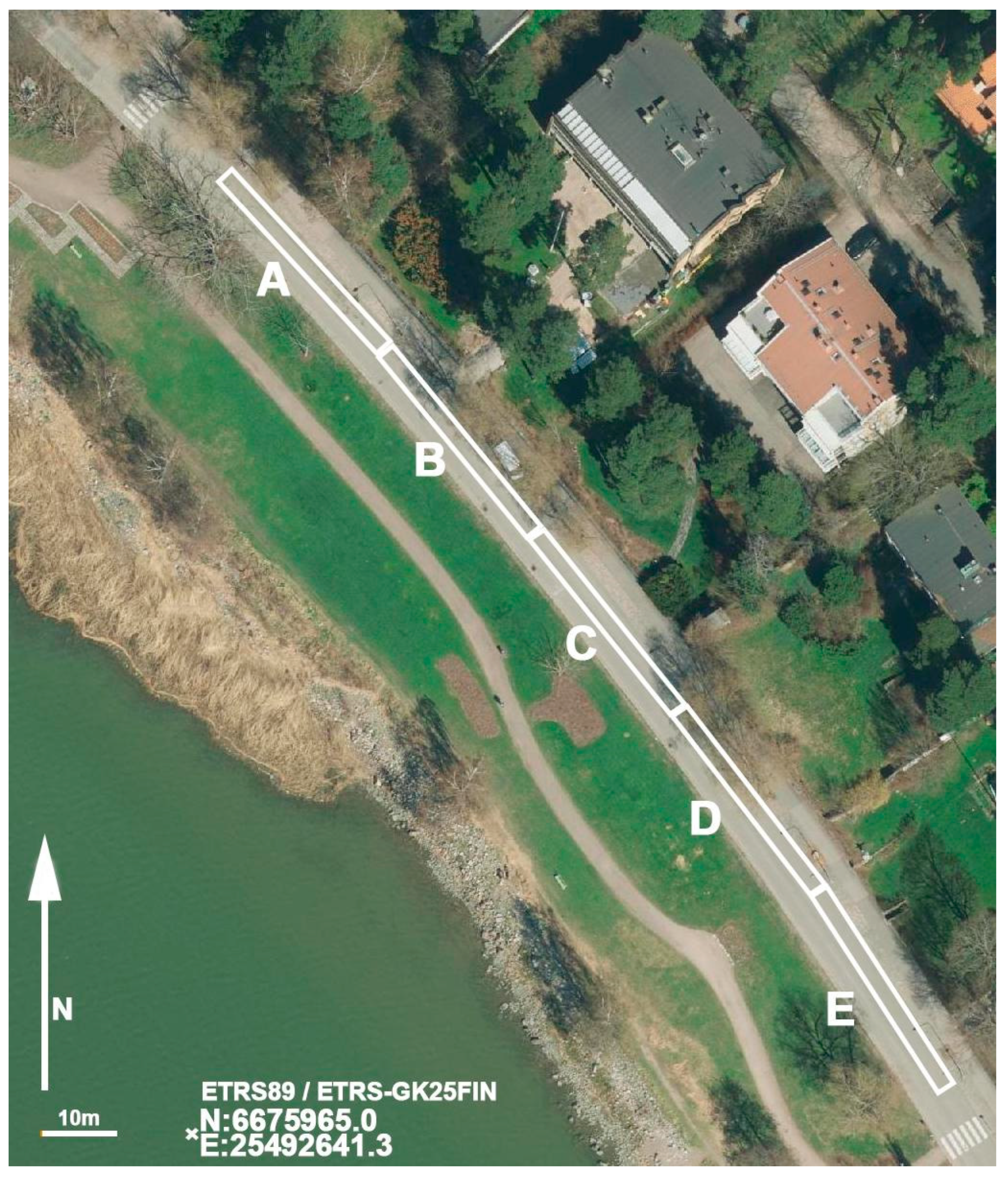
2.1. Measurement Area and Conditions

Mobile measurements were performed two times on a street called Munkkiniemenranta, in Helsinki, Finland. Munkkiniemenranta is a quiet, 1 km long, sub-urban road. When heading northwest, Munkkiniemenranta is sided by a park and the seashore on the left-hand side, and the road lighting instalment and a road verge with trees on the right-hand side. Most of the trees were taller than the mounting height of the luminaires (8.0 m), and in the year 2015, the branches of the trees were severely occluding the road lighting. Both measurements were performed at night when the road surface was illuminated solely by the road luminaires. The measurement vehicle was operated with only the parking lights on. Hence, the vehicle’s effect on the road surface luminance was negligible. As the luminaires were the same luminaires during both of the measurements, there was no measurable change in the spectral power distribution that would have affected the luminance measurement. Furthermore, the measured road surface luminance distributions were compared in relative metrics. Hence, the effect of dimming or aging of the luminaires was also negligible. The conditions on the road surface were dry during both of the measurements, and the effect of background illumination from the surrounding environment was insignificant.
The first measurement was done in September 2015, and the second measurement in April 2019. During the summer of 2018, the trees along Munkkiniemenranta were pruned by the municipality of Helsinki. Five segments of the street were selected for surface luminance analysis. Each segment was the lane on the right-hand side when heading in the northwest direction. Longitudinally, each segment was the area between two adjacent luminaires. The segments were adjacent, creating the area of the right-hand lane between six consecutive luminaires when combined. Figure 1 presents the area of measurement divided into road segments (A–E). The luminaires in the measurement area were 8450 lumen AEC Illuminazione LED luminaires with a longitudinal installation distance of 33 metres.

2.2. Measurement System and Data Processing

The mobile mapping system (MMS) used was a Trimble MX2, which is a vehicle-mounted and geopositioned measurement system that combines panoramic photometry and laser scanning. In Trimble MX2, the geopositioning is performed by the Trimble AP20 GNSS–Inertial System, and the point cloud is scanned with two SLM–250 Class 1 laser heads, which can collect 72,000 points per second. The range of the laser scanning is up to 250 m, and according to the producer, the ranging accuracy of the laser scanning subsystem is ± 1 cm at 50 m for a Kodak white card [32]. However, the range accuracy was not measured or assessed in our experimental environment.
In the first and second measurements, the road surface luminance was measured with Ladybug3 and Ladybug5 panoramic camera systems, respectively. Both camera systems had been radiometrically calibrated under laboratory conditions using an Optronic Laboratories Inc., model 455–6–1 for the reference luminance and a Konica Minolta CS–2000 spectroradiometer as a luminance meter [33]. The luminance values were interpreted from the camera R (red), G (green), and B (blue) values with the factor obtained in the calibration, and Equation (1) from the IEC [34] standard:
Lr = 0.2126R + 0.7152G + 0.0722B
During the measuring, images were captured at 2 metre intervals, and the maximum measurement velocity was 10 m/s. In post processing, the image RGB (red, green, blue) values were registered into the laser scanned point cloud by visually interpreting the point cloud features when superimposed on the images. This is called the interactive orientation method [35,36,37,38]. The interactive orientation method was first applied to data collected during the daytime in order to obtain orientation settings for the nighttime data. Finally, the RGB values were calculated as absolute luminance values applying Equation (1) and a camera-specific calibration constant, and registered as a scalar for each point cloud point. The average point density on the road surface was 1450 points per square metre.
For noise reduction, the analysed road surface areas’ luminance values were median filtered with a diameter of 1.0 metre. Hence, each point had the median luminance value among the points within a 0.5 metre distance of itself. We chose to use the metrics overall uniformity, Uo, and longitudinal uniformity, Ui, to describe the lighting quality. Uo is the ratio between the lowest luminance and the average luminance within the road segment, and Ui is the ratio of the lowest luminance to the highest luminance on the centre line of the measured lane. The descriptions for these measurements are from the European CEN technical report for road lighting, and they are in use in Finnish road lighting regulations [13]. Furthermore, both of these measures are relative measures. Thus, they can be compared despite the age-dependent luminous flux output decrease in luminaires. The measurement area on the Munkkiniemenranta road is classified as road class ME5 according to Finnish road lighting design regulations. In the ME5 class, the target values for Uo and Ui are 0.35 and 0.40, respectively.
The change in the amount of light-occluding vegetation between the years 2015 and 2019 was assessed applying a voxel grid. For each road segment A–E, the space between the road surface and the mounting height of the light sources was sectioned from the point cloud for analysis. For each sub-sectioned point cloud, a voxel grid was created. The voxel grid was created applying a Python program. The program first searched for the boundaries of the sub-sectioned point cloud and created a bounding box. This bounding box was then divided into voxels with a chosen edge length. The voxel grid was populated with the sub-sectioned point cloud, and then the voxel grid was systematically browsed through voxel by voxel. If a voxel contained any number of points it was assigned a binary value 1, and if a voxel contained no points it was assigned a binary value 0. The number of voxels with any number of scanned points in them was considered the measure for the occluding vegetation. In other words, the threshold of occupancy was one for the voxels that were considered light occluding, and the number of occluding voxels between the road surface and the height of the light source was the measure of occlusion. Finally, the numbers of occluding voxels from the year 2015 and the year 2019 were compared. Measuring the volume or biomass of vegetation by laser-scanning is widely studied, and a variety of voxel sizes are suggested depending on the measurement application [39,40,41,42,43,44,45,46,47,48]. In this study, we chose to test cubic voxels with edge lengths of 0.02 m, 0.05 m, 0.10 m, and 0.40 m in order to assess how the voxel cell size affects the calculation of occluding vegetation. When measuring vegetation volume or biomass, the occlusion is often a challenge. In our study, however, the occlusion is exactly the phenomenon we want to measure, and we consider the calculation described above suitable for estimating the layers of occluding vegetation.
In this study, the point cloud sectioning was performed manually in point cloud editing software CloudCompare. We were able to detect every point in the space between the light source and the lane surface as vegetation, since this experimental area was witnessed by us in situ. We identified that the only illumination-blocking features in the measurement area were the tree branches. For large areas, more automated vegetation detection should be considered [49,50,51,52]. For this study, however, this manual method was usable, as our main purpose was to simply identify if there is any sort of correlation between the road surface luminance distribution and the number of occluding voxels between the luminaire mounting height and the road surface. For clarification, luminance values were not calculated to or from the voxel grid at any point. The illumination engineering measures overall luminance uniformity and longitudinal luminance uniformity were calculated from the MMS measurements. Both of these luminance uniformity measures reduce to a single relative value for each road segment, which is the road surface between two adjacent luminaires. The voxel grid was created only for the occluding points, and the number of occluding voxels was considered the measure of occlusion for each road segment, which is the area between two adjacent luminaires. The luminance uniformities and the occlusion measures were then compared.

3. Results

3.1. Overall and Longitudinal Luminance Uniformities

The measured values for Uo and Ui before (2015) and after (2019) roadside vegetation pruning are presented in Table 1.
Figure 2 illustrates the pseudo-coloured luminance values on the road surface for the whole area of measurement before (2015) and after (2019) tree pruning.
Figure 3 presents a visualisation of the measured vegetation directly from the side of the measurement area and from diagonally above the measurement area. In the laser scanned point clouds before the pruning, the lower branches block more laser scans and the canopy was not mapped. Conversely, the laser scans after the pruning penetrate to the upper branches. More obviously, the removed lower branches and full trees can easily be detected when comparing the old and new point clouds.

3.2. Occluding Voxel Analysis

Table 2 presents the number of voxels that encompassed light-occluding vegetation for the measurements conducted before (2015) and after (2019) the roadside tree pruning. Furthermore, Table 2 presents the relative change in the number of voxels that encompassed light-occluding vegetation between the measurements conducted in 2015 and 2019. All of the voxel numbers are presented for road segments A–E, and for cubic voxels with edge lengths of 0.02, 0.05, 0.1, and 0.4 m.
The number of voxels with at least one scanned point of vegetation decreases as the size of the voxel increases.

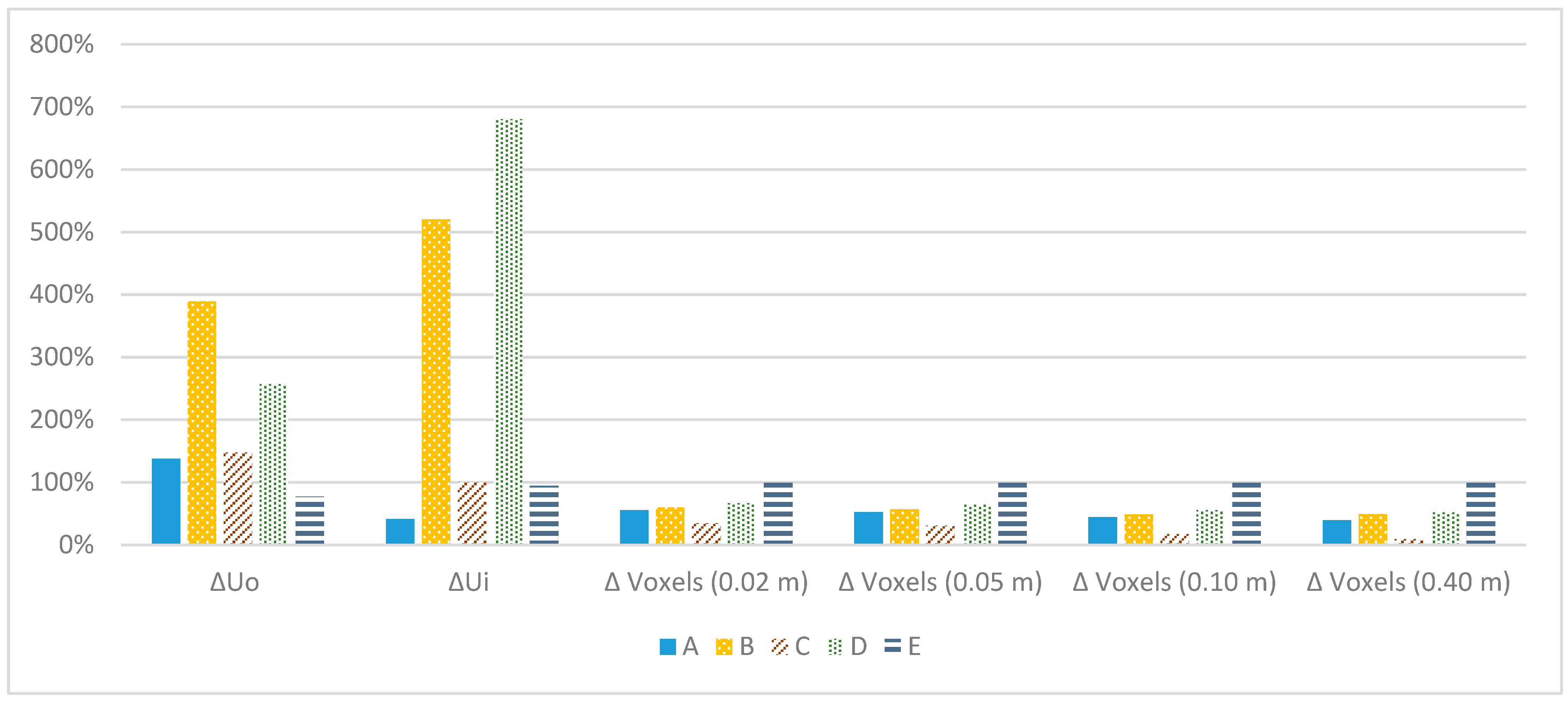
3.3. Occluding Voxels and Luminance Uniformity Comparison

Table 3 presents the absolute value of the change percentage in overall uniformity, longitudinal uniformity, and the number of occluding voxels between the measurements conducted in 2015 and 2019 for each road segment A–E. Figure 4 presents the same values as a column graph.
The decrease in vegetation voxels correlates with improved luminance uniformity values for road segments A–D. For road segment E, vegetation removal also correlates with improved luminance uniformities but not in the same proportion as with road segments A–D. This may be explained by the fact that there was very little occluding vegetation in the 2015 measurement to begin with, and all of it was removed before the 2019 measurement. Hence, the relative number of removed voxels encompassing vegetation was 100% even though there was not that much room for improvement in the luminance uniformity values.

4. Discussion

In this study, we presented a measurement system and a workflow to assess the road lighting-occluding effect of roadside vegetation. In particular, we described a case in which we used a workflow involving a change analysis of the road surface luminance measures for the overall uniformity and longitudinal uniformity measured before and after roadside vegetation pruning. Applying the developed workflow, we verified the improvement in road surface overall and longitudinal luminance uniformities after vegetation pruning.
The authors deem the presented system to be an excellent utility for road lighting measurements. Compared to static measurements, mobile measuring enables fast coverage and data capture of large road or street entireties. With the presented system, the result is a three-dimensional luminance point cloud. The 3D luminance models are undeniably more versatile than the conventional 2D luminance images. Each measured luminance point is geo-referred and in scale, which is not possible with 2D imaging luminance photometry. For the specific case in this study—the verification of improvement in road surface luminance uniformities—the presented measurement system performed very well. Furthermore, the amount of vegetation removed between 2015 and 2019 was analysed applying a voxel grid. The amount of removed vegetation was compared to the improved overall luminance uniformity and longitudinal uniformity values. A correlation was found between these metrics. However, more research is needed to verify the correlation. Moreover, we applied a manual method for point cloud sectioning and occluding voxel detection. The manual method was manageable for our usability study in a limited area. For practical mobile mapping applications, these manual procedures are not feasible, and automation should be considered both for vegetation detection and for the division of measured area. For vegetation detection and feature extraction, machine learning tools such as support vector machines, associative Markov networks, or supervised classification could be applied [48,49,50]. For road area sectioning, classification based on proximity of known road coordinates, and raster image processing techniques could be useful [51].
However, the presented system is not without shortcomings. Firstly, the image capturing of the presented measurement system does not fully follow the guidelines of any road lighting measurement standard. It would naturally be possible to modify the MMS to follow the standards. In this study, this kind of modification would have drastically reduced the point density and accuracy of the point cloud. The authors considered this would have been counter-innovative and decided to use the mobile mapping system at its highest settings possible for the conditions. Likewise, the measurement standard could be updated to include the versatile possibilities of 3D mobile mapping. Secondly, the dynamics and the signal-to-noise ratio of MMS panoramic cameras are not yet optimal and cannot compete with stationary imaging luminance photometry in this respect. However, these technologies are continuously improving. The authors decided that the technology was developed enough to initiate a scientific conversation about mobile luminance measurement. Soon, the difference between mobile and static measurement quality will be negligible in terms of road surface luminance measurements.
In this study, the geometry of the road environment was measured solely with a laser scanner, and the captured digital images were projected onto the geometry. Urban vegetation has also been mapped using solely camera-based photogrammetry [53]. However, the following aspects encourage the use of laser scanning. Firstly, a laser scanner measures absolute distances, whereas camera-based data are only relative in scale. Secondly, laser scanners are active sensors, which means they can measure the geometry in dark conditions, whereas camera-based photogrammetry always requires an external light source to emit light onto the measured surfaces. Especially when measuring under nighttime conditions, the geometry measurement quality would decrease if only camera-based photogrammetry was used. The third option would be a hybrid method in which the geometry is measured using both laser scanners and camera-based photogrammetry. This has been a favoured method for the daytime terrestrial measurement of built environments [54]. The capabilities of this hybrid method should be assessed in future studies for the measurement of artificially lit road environments.
Urban green areas, trees, and vegetation will become even more emphasised and prominent in the future. The shading and temperature-reducing effect of urban vegetation helps to counter the effects of climate change [14,55]. Furthermore, trees increase the property value [56], potentially reduce crime [57,58], and improve air quality [54]. In terms of traffic infrastructure, street lighting obstruction is not the only negative effect of roadside vegetation. Growing trees can also cause damage to the pavement [59]. Conveniently, the measurement system presented in this study could possibly also map pavement damage, and thus, measure these two negative effects caused by urban vegetation with one measurement.
The emergence of low-cost equipment further increases the feasibility of applying MLS in an increasing number of applications. Jaakkola et al [60] have demonstrated the performance of affordable MLS systems. The reduction of the size and weight of MLS systems has also enabled their installation on UAVs, potentially offering a less occluded viewpoint of the urban environment. Highly portable MLS systems can also be utilised by pedestrians, further increasing their flexibility [61]. Systems that rely on the SLAM principle are also able to operate in GNSS-occluded areas. These developments potentially expand the applicability of MLS-based luminance mapping to tunnels, the undersides of bridges, pedestrian areas etc., depending on the performance and suitability of the imaging sensors in these systems. As 3D mapping and imaging have also been demonstrated in near-consumer-level systems, it can also be argued that to some extent luminance mapping could also be carried out via a crowdsourcing-oriented approach in pedestrian areas, for example.
In addition to road lighting assessments, roadside vegetation mapping has various applications. Moose, deer, and elk collisions correlate with roadside vegetation, as they are browsing sites for Cervidae [62]. On the other hand, roadside vegetation has been found to reduce frustration and aggression in drivers [63]. Furthermore, roadside trees have the potential to reduce light pollution from street luminaires [64]. Due to its positive outcome, roadside vegetation is preferred as long as it can be controlled. The measurement system presented in this study is an optimal utility for control.

5. Conclusions

This study demonstrated a novel and specific application for a mobile mapping system. The presented practice can have a direct effect on traffic safety and energy efficiency as the road lighting can be improved and the roadside vegetation reworked according to the measurements. Furthermore, this study is connected to technological trends such as high-definition 3D semantic maps and even autonomous vehicles, as autonomous vehicles could continuously collect the data for vegetation and luminance analysis. Mobile mapping and digital imaging technologies will inevitably improve. Likewise, accelerated urbanization will set higher demands for semantic 3D maps. Most of the mobile mapping is done during the day. Road lighting measurement is one incentive for nighttime mobile mapping. Simultaneously with the lighting measurements, the nighttime urban environment is measured, and this more general measurement can be used to create 3D nighttime models of the urban environment. However, it is important to note that these technological trends could evolve via complementary routes. The ultimate goal for real-time updated 3D city models representing accurate lighting data among the other imaginable semantic information will be achieved gradually.

Author Contributions

Conceptualization, Mikko Maksimainen. Matti Kurkela, Matti T. Vaaja, Juho-Pekka Virtanen, and H.H.; methodology, Mikko Maksimainen Matti Kurkela, Matti T. Vaaja and Juho-Pekka Virtanen; software, Mikko Maksimainen, Matti Kurkela, Matti T. Vaaja and Juho-Pekka Virtanen; investigation, Mikko Maksimainen. Matti Kurkela, Matti T. Vaaja and Juho-Pekka Virtanen; resources, Hannu Hyyppä and Matti T. Vaaja; data curation, Mikko Maksimainen, and Matti Kurkela; writing—original draft preparation, Mikko Maksimainen. Matti Kurkela, Matti T. Vaaja, and Juho-Pekka Virtanen; writing—review and editing, Mikko Maksimainen, Matti Kurkela, Matti T. Vaaja, Juho-Pekka Virtanen, Arttu Julin, Kaisa Jaalama, and Hannu Hyyppä; visualization, Mikko Maksimainen supervision, Hannu Hyyppä, and Matti T. Vaaja; project administration, Hannu Hyyppä; funding acquisition, Hannu Hyyppä, Kaisa Jaalama, Juho-Pekka Virtanen and Matti T. Vaaja; All authors have read and agreed to the published version of the manuscript.

Funding

This research project was funded by the Academy of Finland and the Centre of Excellence in Laser Scanning Research (CoE–LaSR) (No. 272195, 307362). The Strategic Research Council of the Academy of Finland is acknowledged for financial support for the project “Competence Based Growth Through Integrated Disruptive Technologies of 3D Digitalization, Robotics, Geospatial Information and Image Processing/Computing—Point Cloud Ecosystem (No. 293389, 314312)”.

Acknowledgments

We would like to thank Mitaten Oy for cooperation with the luminance measurement equipment.

Conflicts of Interest

The authors declare no conflict of interest.

References

  1. Payne, D.M.; Fenske, J.C. An analysis of the rates of accidents, injuries and fatalities under different light conditions: A Michigan emergency response study of state police pursuits. Policing 1997, 20, 357–373. [Google Scholar] [CrossRef]
  2. Oya, H.; Ando, K.; Kanoshima, H.A. Research on interrelation between illuminance at intersections and reduction in traffic accidents. J. Light Vis. Environ. 2002, 26, 29–34. [Google Scholar] [CrossRef] [Green Version]
  3. Plainis, S.; Murray, I.J.; Pallikaris, I.G. Road traffic casualties: Understanding the night–time death toll. Inj. Prev. 2006, 12, 125–138. [Google Scholar] [CrossRef] [PubMed] [Green Version]
  4. Sullivan, J.M.; Flannagan, M.J. Determining the potential safety benefit of improved lighting in three pedestrian crash scenarios. Accid. Anal. Prev. 2007, 39, 638–647. [Google Scholar] [CrossRef] [PubMed]
  5. Wanvik, P.O. Effects of road lighting: An analysis based on Dutch accident statistics 1987–2006. Accid. Anal. Prev. 2009, 41, 123–128. [Google Scholar] [CrossRef]
  6. Jackett, M.; Frith, W. Quantifying the impact of road lighting on road safety—A New Zealand Study. IATSS Res. 2013, 36, 139–145. [Google Scholar] [CrossRef] [Green Version]
  7. Yannis, G.; Kondyli, A.; Mitzalis, N. Effect of lighting on frequency and severity of road accidents. Proc. Inst. Civ. Eng. Transp. 2013, 166, 271–281. [Google Scholar] [CrossRef]
  8. Elvik, R. Meta–analysis of evaluations of public lighting as accident countermeasure. Transp. Res. Rec. 1995, 1485, 12–24. [Google Scholar]
  9. de Bellis, E.; Schulte–Mecklenbeck, M.; Brucks, W.; Herrmann, A.; Hertwig, R. Blind haste: As light decreases, speeding increases. PLoS ONE 2018, 13, e0188951. [Google Scholar] [CrossRef] [Green Version]
  10. Hölker, F.; Moss, T.; Griefahn, B.; Kloas, W.; Voigt, C.C.; Henckel, D.; Hänel, A.; Kappeler, P.M.; Völker, S.; Schwope, A.; et al. The dark side of light: A transdisciplinary research agenda for light pollution policy. Ecol. Soc. 2010, 15, 13. [Google Scholar] [CrossRef]
  11. Rodríguez, A.; Burgan, G.; Dann, P.; Jessop, R.; Negro, J.J.; Chiaradia, A. Fatal attraction of short–tailed shearwaters to artificial lights. PLoS ONE 2014, 9, e110114. [Google Scholar] [CrossRef]
  12. The Illuminating Engineering Society of North America. ANSI/IES RP-8-14, Roadway Lighting; The Illuminating Engineering Society of North America: NY, USA, 2014; ISBN 978-0-87995-299-0. [Google Scholar]
  13. European Committee for Standardization (CEN). CEN-EN 13201-3, Road lighting—Part 3: Calculation of Performance; European Committee for Standardization (CEN): Brussels, Belgium, 2015. [Google Scholar]
  14. Pitman, S.D.; Daniels, C.B.; Ely, M.E. Green infrastructure as life support: Urban nature and climate change. Trans. R. Soc. S. Aust. 2015, 139, 97–112. [Google Scholar] [CrossRef]
  15. Nieuwenhuijsen, M.J.; Khreis, H.; Triguero–Mas, M.; Gascon, M.; Dadvand, P. Fifty shades of green. Epidemiology 2017, 28, 63–71. [Google Scholar] [CrossRef] [PubMed]
  16. Chang, C.R.; Li, M.H. Effects of urban parks on the local urban thermal environment. Urban For. Urban Green. 2014, 13, 672–681. [Google Scholar] [CrossRef]
  17. Elsadek, M.; Liu, B.; Lian, Z.; Xie, J. The influence of urban roadside trees and their physical environment on stress relief measures: A field experiment in Shanghai. Urban For. Urban Green. 2019, 42, 51–60. [Google Scholar] [CrossRef]
  18. Huang, Q.; Yang, M.; Jane, H.A.; Li, S.; Bauer, N. Trees, grass, or concrete? The effects of different types of environments on stress reduction. Landsc. Urban Plan. 2020, 193, 103654. [Google Scholar] [CrossRef]
  19. Threlfall, C.G.; Williams, N.S.; Hahs, A.K.; Livesley, S.J. Approaches to urban vegetation management and the impacts on urban bird and bat assemblages. Landsc. Urban Plan. 2016, 153, 28–39. [Google Scholar] [CrossRef]
  20. Jaakkola, A.; Hyyppä, J.; Hyyppä, H.; Kukko, A. Retrieval algorithms for road surface modelling using laser–based mobile mapping. Sensors 2008, 8, 5238–5249. [Google Scholar] [CrossRef] [Green Version]
  21. Lehtomäki, M.; Jaakkola, A.; Hyyppä, J.; Kukko, A.; Kaartinen, H. Detection of vertical pole–like objects in a road environment using vehicle–based laser scanning data. Remote Sens. 2010, 2, 641–664. [Google Scholar] [CrossRef] [Green Version]
  22. Cabo, C.; Kukko, A.; García–Cortés, S.; Kaartinen, H.; Hyyppä, J.; Ordoñez, C. An algorithm for automatic road asphalt edge delineation from mobile laser scanner data using the line clouds concept. Remote Sens. 2016, 8, 740. [Google Scholar] [CrossRef] [Green Version]
  23. Javanmardi, M.; Javanmardi, E.; Gu, Y.; Kamijo, S. Towards high–definition 3D urban mapping: Road feature–based registration of mobile mapping systems and aerial imagery. Remote Sens. 2017, 9, 975. [Google Scholar] [CrossRef] [Green Version]
  24. Balado, J.; González, E.; Arias, P.; Castro, D. Novel Approach to Automatic Traffic Sign Inventory Based on Mobile Mapping System Data and Deep Learning. Remote Sens. 2020, 12, 442. [Google Scholar] [CrossRef] [Green Version]
  25. Holopainen, M.; Kankare, V.; Vastaranta, M.; Liang, X.; Lin, Y.; Vaaja, M.T.; Yu, X.; Hyyppä, J.; Hyyppä, H.; Kaartinen, H.; et al. Tree mapping using airborne, terrestrial and mobile laser scanning—A case study in a heterogeneous urban forest. Urban For. Urban Green. 2013, 12, 546–553. [Google Scholar] [CrossRef]
  26. del–Campo–Sanchez, A.; Moreno, M.; Ballesteros, R.; Hernandez–Lopez, D. Geometric Characterization of Vines from 3D Point Clouds Obtained with Laser Scanner Systems. Remote Sens. 2019, 11, 2365. [Google Scholar] [CrossRef] [Green Version]
  27. Holopainen, M.; Vastaranta, M.; Kankare, V.; Kantola, T.; Kaartinen, H.; Kukko, A.; Vaaja, M.T.; Hyyppä, J.; Hyyppä, H. Mobile terrestrial laser scanning in urban tree inventory. In Proceedings of the 11th International Conference on LiDAR Applications for Assessing Forest Ecosystems (SilviLaser 2011), Hobart, Australia, 16–20 October 2011. [Google Scholar]
  28. Wu, J.; Yao, W.; Polewski, P. Mapping individual tree species and vitality along urban road corridors with LiDAR and imaging sensors: Point density versus view perspective. Remote Sens. 2018, 10, 1403. [Google Scholar] [CrossRef] [Green Version]
  29. Vaaja, M.T.; Kurkela, M.; Virtanen, J.-P.; Maksimainen, M.; Hyyppä, H.; Hyyppä, J.; Tetri, E. Luminance–corrected 3D point clouds for road and street environments. Remote Sens. 2015, 7, 11389–11402. [Google Scholar] [CrossRef] [Green Version]
  30. Vaaja, M.T.; Kurkela, M.; Maksimainen, M.; Virtanen, J.-P.; Kukko, A.; Lehtola, V.V.; Hyyppä, J.; Hyyppä, H. Mobile mapping of night–time road environment lighting conditions. Photogramm. J. Finland 2018, 26, 1–7. [Google Scholar] [CrossRef]
  31. Helsingin Karttapalvelu (Helsinki Map Service). Available online: http://kartta.hel.fi (accessed on 18 March 2020).
  32. Trimble MX2 Mobile Mapping System. Available online: http://www.webcitation.org/6sc5p4MvX (accessed on 18 March 2020).
  33. Kurkela, M.; Maksimainen, M.; Vaaja, M.T.; Virtanen, J.-P.; Kukko, A.; Hyyppä, J.; Hyyppä, H. Camera preparation and performance for 3D luminance mapping of road environments. Photogramm. J. Finland 2017, 25, 1–23. [Google Scholar] [CrossRef]
  34. International Electrotechnical Commission. Multimedia Systems and Equipment–Colour Measurement and Management-Part 2-1: Colour Management—Default RGB Colour Space—sRGB; IEC 61966-2-1; International Electrotechnical Commission: Geneva, Switzerland, 1999. [Google Scholar]
  35. Barber, D.; Mills, J.; Bryan, P.G. Laser Scanning and Photogrammetry—21st Century Metrology. Int. Arch. Photogramm. Remote Sens. Spat. Inf. Sci. 2002, 34, 360–366. [Google Scholar]
  36. Rönnholm, P.; Honkavaara, E.; Litkey, P.; Hyyppä, H.; Hyyppä, J. Integration of laser scanning and photogrammetry. Int. Arch. Photogramm. Remote Sens. Spat. Inf. Sci. 2007, 36, 355–362. [Google Scholar]
  37. Abdelhafiz, A.; Riedel, B.; Niemeier, W. Towards a 3D true colored space by the fusion of laser scanner point cloud and digital photos. In Proceedings of the ISPRS Working Group V/4 Workshop 3D–ARCH 2005, Mestre-Venice, Italy, 22–24 August 2005. [Google Scholar]
  38. Rönnholm, P.; Hyyppä, H.; Hyyppä, J.; Haggrén, H. Orientation of airborne laser scanning point clouds with multi-view, multi-scale image blocks. Sensors 2009, 9, 6008–6027. [Google Scholar] [CrossRef] [PubMed] [Green Version]
  39. Moskal, L.M.; Zheng, G. Retrieving forest inventory variables with terrestrial laser scanning (TLS) in urban heterogeneous forest. Remote Sens. 2012, 4, 1–20. [Google Scholar] [CrossRef] [Green Version]
  40. Hauglin, M.; Astrup, R.; Gobakken, T.; Næsset, E. Estimating single–tree branch biomass of Norway spruce with terrestrial laser scanning using voxel–based and crown dimension features. Scand. J. For. Res. 2013, 28, 456–469. [Google Scholar] [CrossRef]
  41. Wu, B.; Yu, B.; Yue, W.; Shu, S.; Tan, W.; Hu, C.; Huang, Y.; Wu, J.; Liu, H. A voxel–based method for automated identification and morphological parameters estimation of individual street trees from mobile laser scanning data. Remote Sens. 2013, 5, 584–611. [Google Scholar] [CrossRef] [Green Version]
  42. Yao, W.; Fan, H. Automated detection of 3D individual trees along urban road corridors by mobile laser scanning systems. In Proceedings of the International Symposium on Mobile Mapping Technology, Tainan, Taiwan, 6 May 2013. [Google Scholar]
  43. Bienert, A.; Hess, C.; Maas, H.G.; Von Oheimb, G. A voxel–based technique to estimate the volume of trees from terrestrial laser scanner data. In Proceedings of the International Archives of the Photogrammetry, Remote Sensing & Spatial Information Sciences Commission V Symposium, Riva del Garda, Italy, 23–25 June 2014. [Google Scholar]
  44. Cifuentes, R.; Van der Zande, D.; Farifteh, J.; Salas, C.; Coppin, P. Effects of voxel size and sampling setup on the estimation of forest canopy gap fraction from terrestrial laser scanning data. Agric. For. Meteorol. 2014, 194, 230–240. [Google Scholar] [CrossRef]
  45. Jalonen, J.; Järvelä, J.; Virtanen, J.-P.; Vaaja, M.T.; Kurkela, M.; Hyyppä, H. Determining characteristic vegetation areas by terrestrial laser scanning for floodplain flow modeling. Water 2015, 7, 420–437. [Google Scholar] [CrossRef] [Green Version]
  46. Liang, X.; Kankare, V.; Hyyppä, J.; Wang, Y.; Kukko, A.; Haggrén, H.; Yu, X.; Kaartinen, H.; Jaakkola, A.; Guan, F.; et al. Terrestrial laser scanning in forest inventories. ISPRS J. Photogramm. Remote Sens. 2016, 115, 63–77. [Google Scholar] [CrossRef]
  47. Grau, E.; Durrieu, S.; Fournier, R.; Gastellu–Etchegorry, J.P.; Yin, T. Estimation of 3D vegetation density with Terrestrial Laser Scanning data using voxels. A sensitivity analysis of influencing parameters. Remote Sens. Environ. 2017, 191, 373–388. [Google Scholar] [CrossRef]
  48. Kükenbrink, D.; Schneider, F.D.; Leiterer, R.; Schaepman, M.E.; Morsdorf, F. Quantification of hidden canopy volume of airborne laser scanning data using a voxel traversal algorithm. Remote Sens. Environ. 2017, 194, 424–436. [Google Scholar] [CrossRef]
  49. Loghin, A.; Oniga, V.E.; Giurma–Handley, C. 3D Point Cloud Classification of Natural Environments Using Airborne Laser Scanning Data. Am. J. Eng. Res. 2018, 7, 191–197. [Google Scholar]
  50. Lucas, C.; Bouten, W.; Koma, Z.; Kissling, W.D.; Seijmonsbergen, A.C. Identification of linear vegetation elements in a rural landscape using LiDAR point clouds. Remote Sens. 2019, 11, 292. [Google Scholar] [CrossRef] [Green Version]
  51. Weinmann, M.; Weinmann, M.; Mallet, C.; Brédif, M. A classification–segmentation framework for the detection of individual trees in dense MMS point cloud data acquired in urban areas. Remote Sens. 2017, 9, 277. [Google Scholar] [CrossRef] [Green Version]
  52. Hůlková, M.; Pavelka, K.; Matoušková, E. Automatic classification of point clouds for highway. Acta Polytech. 2018, 58, 165–170. [Google Scholar] [CrossRef]
  53. Seiferling, I.; Naik, N.; Ratti, C.; Proulx, R. Green streets—Quantifying and mapping urban trees with street–level imagery and computer vision. Landsc. Urban Plan. 2017, 165, 93–101. [Google Scholar] [CrossRef]
  54. Julin, A.; Jaalama, K.; Virtanen, J.-P.; Maksimainen, M.; Kurkela, M.; Hyyppä, J.; Hyyppä, H. Automated Multi–Sensor 3D Reconstruction for the Web. ISPRS Int. J. Geo-Inf. 2019, 8, 221. [Google Scholar] [CrossRef] [Green Version]
  55. Van Renterghem, T.; Hornikx, M.; Forssen, J.; Botteldooren, D. The potential of building envelope greening to achieve quietness. Build. Environ. 2013, 61, 34–44. [Google Scholar] [CrossRef] [Green Version]
  56. Pandit, R.; Polyakov, M.; Tapsuwan, S.; Moran, T. The effect of street trees on property value in Perth, Western Australia. Landsc. Urban Plan. 2013, 110, 134–142. [Google Scholar] [CrossRef]
  57. Kondo, M.C.; Han, S.; Donovan, G.H.; MacDonald, J.M. The association between urban trees and crime: Evidence from the spread of the emerald ash borer in Cincinnati. Landsc. Urban Plan. 2017, 157, 193–199. [Google Scholar] [CrossRef] [Green Version]
  58. Eisenman, T.S.; Churkina, G.; Jariwala, S.P.; Kumar, P.; Lovasi, G.S.; Pataki, D.E.; Weinberger, K.R.; Whitlow, T.H. Urban trees, air quality, and asthma: An interdisciplinary review. Landsc. Urban Plan. 2019, 187, 47–59. [Google Scholar] [CrossRef]
  59. Mullaney, J.; Lucke, T.; Trueman, S.J. A review of benefits and challenges in growing street trees in paved urban environments. Landsc. Urban Plan. 2015, 134, 157–166. [Google Scholar] [CrossRef]
  60. Jaakkola, A.; Hyyppä, J.; Kukko, A.; Yu, X.; Kaartinen, H.; Lehtomäki, M.; Lin, Y. A low-cost multi-sensoral mobile mapping system and its feasibility for tree measurements. ISPRS J. Photogramm. Remote Sens. 2010, 65, 514–522. [Google Scholar] [CrossRef]
  61. Nocerino, E.; Menna, F.; Remondino, F.; Toschi, I.; Rodríguez-Gonzálvez, P. Investigation of indoor and outdoor performance of two portable mobile mapping systems. Proceednings of the Videometrics, Range Imaging, and Applications XIV, Munich, Germany, 26–27 June 2017. [Google Scholar]
  62. Tanner, A.L.; Leroux, S.J. Effect of roadside vegetation cutting on moose browsing. PLoS ONE 2015, 10, e0133155. [Google Scholar] [CrossRef] [PubMed] [Green Version]
  63. Cackowski, J.M.; Nasar, J.L. The restorative effects of roadside vegetation: Implications for automobile driver anger and frustration. Environ. Behav. 2003, 35, 736–751. [Google Scholar] [CrossRef] [Green Version]
  64. Gaston, K.J.; Davies, T.W.; Bennie, J.; Hopkins, J. Reducing the ecological consequences of night-time light pollution: Options and developments. J. Appl. Ecol. 2012, 49, 1256–1266. [Google Scholar] [CrossRef] [PubMed] [Green Version]
Figure 1. The full area of measurement and the analysed road surface segments A, B, C, D, and E. [31] (Orthophotograph © Helsinki City Survey Department, 2017).
Ijgi 09 00455 g001
Figure 2. Pseudo-coloured luminance values on the road surface for the whole area of measurement before (2015) and after (2019) tree pruning.
Ijgi 09 00455 g002
Figure 3. Visual assessment of the roadside vegetation. From the side (a.) and diagonally above (b.). Pseudo-coloured maps of the height (m) or the z-axis in local coordinates.
Ijgi 09 00455 g003
Figure 4. The absolute value of the change percentage in overall uniformity Uo, longitudinal uniformity Ui, and the number of occluding voxels (edge lengths: 0.02; 0.05; 0.10; 0.40 m) between the measurements conducted in 2015 and 2019 for each road segment A–E.
Ijgi 09 00455 g004
Table 1. The overall and longitudinal uniformities in the road segments (A–E) on the road surface before and after the vegetation trimming. Furthermore, the relative (rel.) differences between the 2015 and 2019 measurements for the both uniformity measures are presented in their individual columns.
SegmentUo beforeUo afterUo rel. DifferenceUi beforeUi afterUi rel. Difference
A0.240.57137.5%0.290.4141.4%
B0.090.44388.9%0.050.31520.0%
C0.170.42147.1%0.130.26100.0%
D0.140.50257.1%0.050.39680.0%
E0.300.5376.7%0.170.3394.1%
Average0.190.49157.9%0.140.34142.9%
Table 2. The number of voxels that encompass occluding vegetation for the space between the road surface and the mounting height of the light sources in the 2015 and 2019 measurements. The numbers are presented for road segments A–E and cubic voxels with 0.02, 0.05, 0.1, and 0.4 m long edges. The lowest row cluster presents the average number of occluding vegetation among the road segments for voxel size. For each road segment (A–E) and their average, the relative decrease percentage in the number of occluding voxels is presented.
0.02 m0.05 m0.1 m0.4 m
A (2015)11,97210,3356584634
A (2019)536449493672387
–55.2%–52.1%–44.2%–39.0%
B (2015)79,14868,02343,5033909
B (2019)31,99029,66422,2951999
–59.6%–56.4%–48.8%–48.9%
C (2015)22,41219,60212,412933
C (2019)14,66113,59910,331849
–34.6%–30.6%–16.8%–9.0%
D (2015)91,27278,67746,8083836
D (2019)30,48228,43320,9031864
–66.6%–63.9%–55.3%–51.4%
E (2015)18,06315,85610,233944
E (2019)0000
–100.0%–100.0%–100.0%–100.0%
Average (2015)44,573.438,498.623,908.02051.2
Average (2019)16,499.415,329.011,440.21019.8
–63.2%–60.6%–53.0%–49.6%
Table 3. The absolute value of the change percentage in overall uniformity Uo, longitudinal uniformity Ui, and the number of occluding voxels (edge length: 0.02; 0.05; 0.10; 0.40 m) between the measurements conducted in 2015 and 2019 for each road segment A–E.
ABCDE
ΔUo138%389%147%257%77%
ΔUi41%520%100%680%94%
Δ voxels (0.02 m) 55%60%35%67%100%
Δ voxels (0.05 m)52%56%31%64%100%
Δ voxels (0.10 m)44%49%17%55%100%
Δ voxels (0.40 m)39%49%9%51%100%

