Measuring Accessibility to Various ASFs from Public Transit using Spatial Distance Measures in Indian Cities

Department of Architecture and Planning, Visvesvaraya National Institute of Technology, Nagpur 440010, India
*
Author to whom correspondence should be addressed.
ISPRS Int. J. Geo-Inf. 2020, 9(7), 446; https://doi.org/10.3390/ijgi9070446
Submission received: 8 June 2020
/
Revised: 2 July 2020
/
Accepted: 15 July 2020
/
Published: 17 July 2020
(This article belongs to the Special Issue Measuring, Mapping, Modeling, and Visualization of Cities)
Abstract
:Nowadays, accessibility to facilities is one of the most discussed issues in sustainable urban planning. In the current research, two spatial distance accessibility measures were applied to evaluate the accessibility to amenities, services, and facilities (ASFs) from public transit (PT) by walking distance in six Indian cities. The first stage accounts for distance measures using the Euclidean distance with a new methodical approach derived from the built-up area with a spatial resolution of 30 m from Landsat data, and for the network distance method, the actual road distances using OpenStreetMap (OSM) for different threshold ranges of distances were derived. Meanwhile, in the second stage, indicators such as built-up area, network connectivity, and network density with the percentage of ASFs are evaluated and combined for normalization process for ranking the city. The present study assesses the accessibility to various ASFs from PT at city level and explores whether the actual road network access (by measuring distance) in Indian cities is contributing to a high level of accessibility. It adopts a unique approach using statistical tools while assessing both Euclidean and network distances. It models a framework for overall benchmarking in all six cities by ranking them for their accessibility. The results show various scenarios in terms of the rank of cities, which had been strongly affected by distance metrics (Euclidean vs. network) and thus emphasize the careful use of these measures as supporting tools for planning. This facilitates the identification of the local barriers and problems with network access that affect the actual distance. This unique approach can help policymakers to identify the gaps in PT coverage for reaching ASFs. Furthermore, it helps in crucial implementation by strategic planning that can be achieved using these distance criteria.
1. Introduction
For the past five decades, accessibility has been central to physical planning and spatial modelling. Hansen (1959) defined accessibility as the ease of access to a desirable destination by linking land use and activities with the transport network [1]. Later on, researchers called for a paradigm shift from auto mobility-oriented planning to accessibility-oriented planning [2]. Evidence shows that better access to services by feasible modes with less impact on the environment is an influencing factor in achieving sustainable accessibility [3].
In recent years, public transport has become increasingly focused on improvements in sustainability [4]. Improving access to public transit (PT) can be considered as an effective way to reduce the external cost and negative impacts of motorized vehicles [5]. Better access will encourage people to use more environment friendly transportation modes, including walking and cycling. These features that promote various forms of physical activity (such as walking) can be referred to as ’neighborhood walkability’ and they often consider destinations such as retail stores and parks, and community design features such as street connectivity and sidewalk access [6,7].
1.1. Need for Accessibility in Case of India
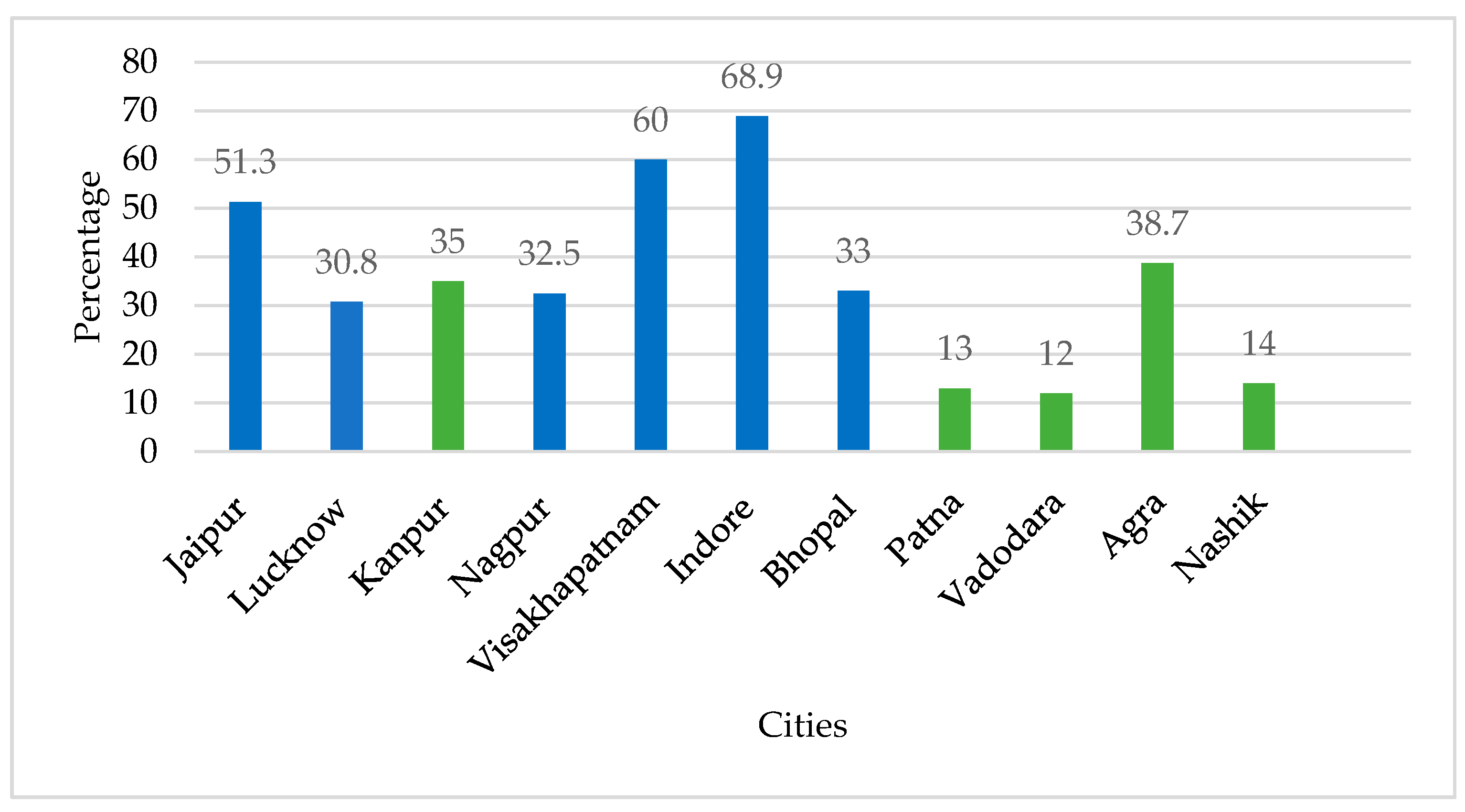
In India over a period of time, despite significant efforts to boost public transport growth in urban areas, the share of buses in total registered vehicles fell from 11.1% in 1951 to 1.1% in 2011 [8]. Similarly, non-motorized transport (NMT) share has declined, and although walking and cycling still account for 33% in most Indian cities, the percentage is declining year after year. On the contrary, in developed nations, with leading examples from London, Berlin and Copenhagen, the renaissance of NMT is taking place, with shares of NMT of about 30% [9]. Focusing on these incumbent issues, policies in India are now highlighting the opportunity to bring people and activities closer to PT [10]; and even targeting the improvement of infrastructure for cycling, walking and the city’s overall network coverage [11]. This will help in improving NMT infrastructure, thereby increasing access to various services to reach PT.
The distance that people walk to bus stops plays a crucial role in allowing the best use of public transport. The higher the percentage of people living or working close to the transit, the greater the probability of them using the service [12]. Studies in developed nations are rapidly focusing on this issue, by measuring accessibility in various cities and metropolitan areas with spatial dimensions in reaching public transit using walk scores [4,13]. A few other studies on urban intervention for access to various kinds of facilities and services for walkable distances have compared cities globally, irrespective of their size [14], and ranked them [15]. Potential spatial accessibility measures evaluating distance to reach PT and other utility services have been little explored in cities in the Global South, especially in India. The pursuit of connecting various services and amenities to PT constitutes an important objective in recent planning in Indian cities.
Previous investigations of several studies of accessibility using geographical information system GIS were conducted at the city level, associated were dealing with accessibility to jobs, connections using public transport, reaching the nearest transit from workplace [15,16,17]. But the focus on other amenities and services connecting to PT is very rare at the city level—these studies have so far focused on the neighborhood-level [18]. Only a few studies have been conducted at the city level, such as the one conducted in Pune metropolitan area in India, which revealed that 41% of school children do not have access to public transit [19]. Many students in India are restricted to their society schools because of inadequate PT services in some parts of the city, as lower-income families cannot afford private transport modes to reach schools at a far distance [20]. Implementing geospatial technologies towards health access in numerous developed nations has become widespread, but the use of these approaches in India has been fairly slow [21]. Only a small amount of research has been carried out in spatially connecting access to health care infrastructure with residents and the road network in India [22].
There are many methods to measure cities’ accessibility, but they cannot be generalized for all cities and towns around the world, since accessibility is affected by the local network, data quality and local context [23]. An alternative approach is needed to tackle unique and specific issues concerning settlements in India. Accessibility is well established at the neighborhood scale, but often a city is not a homogeneous entity in terms of dynamics, considering land-use patterns and network. In this study, a comprehensive cumulative accessibility score and index of cities is conducted. Additionally, spatial mapping of the city network and built-up area is taken into consideration, along with discrete interventions.
The present research is conducted in six Indian cities with a population of more than 1.5 million. Therefore, the scope of the present study is to assess the accessibility to various amenities, services, and facilities (ASFs) from PT at the city level and to explore whether the actual road network access (by measuring distance) in Indian cities is contributing to a high level of accessibility. The method in this study is more flexible and easier to use, and it helps to provide useful information for decision-making on improving accessibility to ASFs from PT. It also provides efficiency from a spatial perspective and thus assists policy makers.
1.2. Research Question and Hypothesis
Access to various services and amenities is recognized as an important facilitator and it becomes a primary concern in any accessibility plans. To integrate various services, geographic access plays an important role worldwide. In order to understand this importance, three research questions were studied: (1) what is the role of various indicators of spatial accessibility? (2) how can spatial accessibility in Indian cities be measured using combination of various indicators? and (3) how is accessibility between ASFs and PT measured? This study is an attempt to understand whether Indian cities have high access level, particularly in cities with a population of more than 1.5 million, i.e., million-plus cities in India. The components that relate to accessibility, such as built-up area and network density, were also included in this study. It is necessary to understand whether cities have better accessibility and whether the accessibility of ASFs to PT is high and can be measured at the entire city level. Indicators such as built-up area, network density and connectivity are combined to know the levels of cities’ accessibility. Two hypotheses were framed to identify levels of spatial accessibility based on distance criteria in the case of Indian cities: (1) distance of ASFs from PT plays a crucial role in defining cities accessibility. (2) Spatial accessibility in a city can be measured and evaluated based on various indicators.
This paper is organized into six parts—introduction, literature review, case selection and data collection, data analysis, results, discussions, and conclusions. The introduction presents the importance of accessibility planning and factors influencing accessibility. It further states the need to conduct the study in Indian cities for measuring accessibility, particularly to ASFs from PT. The second section describes the literature review by identifying various measures of accessibility with reference to cases of developed nations, which helps in the selection of indicators. The third section elaborates on the selection of cities and data collection. The fourth section presents the data analysis based on parameters including a data quality check, measuring accessibility by distance measures, detour index, normalization, etc. In the fifth and sixth sections, the results are presented, followed by a detailed discussion on the output of study. The last section makes the concluding remarks for the study.
2. Literature Review
There are various approaches for achieving sustainable urban development through a city’s form. One of the key aspects of sustainability focused on nowadays is accessibility, namely how accessible green spaces, jobs and services are to communities and how interconnected they are with walking and cycling facilities [24]. Accessibility mostly depends on density and transport linkages, which in turn depend on land use distribution [25]. It is necessary to develop accessibility for reasonable walking distance in cities of developing countries, because of a high level of mixed-use development patterns [26]. Cities which are well designed allow people to have high levels of access to services and facilities, encouraging proximity and social interactions. This permits a range of public transport services and is less consumptive in terms of resource use per person [27]. Evidence shows that better access to services by feasible public transport has a less negative impact on the environment [3]. Therefore, the availability of public transport must be made close to the activities, whereby accessing them becomes much easier [28]. Many cities concentrate on improving access to PT, which often involves some walking or cycling interventions to connect from the origin to destination of the trip, and this leads to improved last-mile connectivity [29]. It interlinks the accessibility of one parameter to another, as shown in Figure 1, for example improving accessibility towards walking and cycling to provide more local access. It will have a direct impact on public transport’s access and indirectly affects commuting distance for jobs, services, and recreation and health facilities. Overall, it requires policies for improving mobility with mode, road and pathway network, design and encouraging non-motorized vehicles in an urban area.
2.1. Measuring Accessibility: Methods and Techniques
Measuring accessibility is an essential component in many transport and accessibility plans, as it gives evidence for preparing guidelines and policies while also creating accessibility index [30]. Accessibility measures often focus primarily on one specific mode or a limited set of destination types, such as jobs. Accessibility measures are classified based on two main aspects, i.e., travel behavior and potential availability of opportunities [31]. These are divided into four important categories of active measures: (i) gravity-based, (ii) topology-based, (iii) distance-based, and (iv) utility-based [32]. All these measures are now currently focusing on the growing interest in spatial data technologies and are expected to have many precise results [33]. Studies are now widely carried out using geographical information system (GIS)-based mapping of accessibility to public transit [13,32,34]. Moreover, studies focusing on access to health care and travel time to hospitals are now widespread, and the distance to shops and cultural facilities were found to be an important factor [35].
Measures are described by a set of parameters concerning (1) a population-based spatial unit, (2) an accessibility measure, and (3) a distance measure chosen for measuring accessibility [36]. While assessing geographic accessibility, the use of these criteria may produce different results depending on the distance measure selected. Some researchers explored the geographical accessibility of health facilities by calculating the accessibility to the nearest facility using the shortest Euclidean distance, (extension of Minkowski distance measures), network distance or a combination of distance types [35,36]. Whereas few studies used the choice of Manhattan distance and Euclidean distances [37], but investigations later concluded that comparing Euclidean distance and network distance is more reliable [38,39]. Moreover, considering network distance measures further helps in the decision-making process for resource location and construction of new facilities [40].
Furthermore, in various countries, accessibility is tested using multiple accessibility instruments (AI). One such is Spatial Network Analysis for Multimodal Urban Transport Systems (SNAMUTS) in Australia, where it uses geographical information systems (GIS) tools to assess the linkage between the public transport network by clustering land use and visualizing its strengths and weaknesses across the metropolitan areas by spatial mapping. Spatial Network Analysis of Public Transport Accessibility Systems (SNAPTA) in the United Kingdom contributes to identifying barriers and creates an accessibility index to integrate NMT with PT. It was developed with an idea to identify "whether, at a reasonable cost and with reasonable ease, one can reach to services and activities". A few studies, such as Isochrones Maps to Facilities (IMaFa) in Spain and Method for Arriving at Maximus Recommendable Size of Shopping Centre (MaReSi) in Norway, measure accessibility to activities such as shopping centres. The IMaFa tool calculates services in a buffer area using Euclidean distance and travel times along a network performed in GIS. MaReSi calculates services by using walking and bicycle distances from dwelling to shopping center within 1–2 km by road distance to the site [41].
Land Use and Public Transport Accessibility Index (LUPTAI), developed in Australia, aims to quantify access by walking and the public transport network to destinations such as education, health shopping, jobs. LUPTAI considers walking in two ways: whether it is a single mode of access for a destination considering walking distances, i.e., (400, 600, 800, 1000 and 1200 m) or a mode of access to public transport i.e., (0–20, 20–40 and 40 plus min) [42]. Tools like Walk Score® (www.walkscore.com) developed in the U.S.A tests access to the nearest public transit and services such as shopping and educational resources (schools and libraries) by walk scores and this tool is available in the public domain [6]. All these instruments are known for interventions that cover the aspects of physical distance, travel time and travel cost.
By comparing all these AI tools irrespective of their strength and weakness, a study showed that instruments using spatial separation measured by an existing network rather than gravity measures have a high level of communication value on ground level, meaning that even non-expert users can easily interpret network flows or link connectivity [43]. Therefore, the presented study adopts spatial accessibility measures used by researchers in the past [36,37,44]. However, these studies have not often been conducted in developing nations like India. Hence, there is little quantitative work on the accessibility of Indian cites done previously. This study uses spatial data for developing an index to compare accessibility in Indian cities, by excluding cost and time factors, as they create complexity for comparing various cities. Here, the distance from ASFs is investigated using both Euclidean and network distance, and we compare both techniques within and among the cities in the Indian context.
2.2. Selection of Indicators
In a few studies, the macro-scale evaluation considered land use and land cover, job density and population density [44,45]. However, Indian demographic information corresponds to the 2011 census, and authoritarian land use plans are more than a decade old. This study, therefore, only includes built-up area extracted from Landsat 8 images, and thus the ASFs mapped are from year 2018–2019.
A comprehensive spatial accessibility assessment would help policymakers to take appropriate actions for improving overall accessibility in cities. Relevant indicators are selected from various literature regarding mobility/walkability [46,47,48], for land cover [49], and for network density, connectivity [50,51], as shown in Table 1.
The selection of diverse and multifold opportunities will provide a viable option to assess accessibility plans in a much better way. Education, health care, leisure, entertainment activities, and commuting capabilities are commonly seen as the leading demands of urban contemporary life. Unlike economic development infrastructures, social infrastructure includes the facilities and places that primarily serve the specific needs of everyday life [52]. With this understanding, various utilities in developed nations were identified as relating to accessibility to a specific infrastructure, such as health [39,52], parks and green spaces [38,53], schools [54,55], transit [32,56,57,58]. A common goal for these studies was to limit the usage of private vehicles and encourage access to public transit by walking and bicycling. Based on this, various sectors are categorized as ASFs (Table 2). In India, as per guidelines, policies and a few research studies have identified recreation activities as “Amenities” in the urban local bodies act, (Government of India, 1992) [59], while police stations and post offices are considered in the category of "Services" [60]. Education and health are considered in the category of "Facilities" in the 83rd Constitutional Amendment Act (Government of India, 2002), which focuses on universal access [61].
2.3. Identifying Reliable Walking Distance
To measure accessibility using distance, researchers used standard walking distances similar to the planners’ thumb rule, i.e., 400 and 800 m [62,63]. Even the World Bank suggests that bus services should be made available for less than 400 m distance to encourage pedestrians [64]. A few other recommended distances from different literature reviews are shown in Table 3.
Indian policies which encourage accessibility specify ideal distances to access urban facilities and services. The Urban and Regional Development Plans Formulation and Implementation-2015 (URDPFI) guidelines [72] dictate that the ideal distance for facilities and transit must be available within 600 to 800 m. The colour code used for mapping and identifying Euclidean and network distances is shown in Table 4.
3. Methodology
This paper introduces a framework to assess accessibility at a macro level with the help of derived indicators from literature studies for various ASFs from PT, as shown in Figure 2.
3.1. Selection of Cities in India
India’s urban population continues to grow at an unprecedented rate. The majority of new development is occurring in major cities such as the metropolitan (over 4 million inhabitants) and million-plus cities (over 1 million inhabitants), popularly known in India as tier-2 cities [73]. As per Wilber Smith Associates’ report, two types of accessibility indices are developed: (i) Public Transport Accessibility Index and (ii) Service Accessibility Index. Public Transport Accessibility Index is formulated as the inverse of the average distance (in km) to the nearest bus stop/railway station (suburban/metro). The Service Accessibility Index is computed as the percentage of work trips accessible within 15 to 30 minutes for each city. For both the indices, medium category cities, i.e., those that fall in Tier 2 cities, have better accessibility compared to low and high category cities [74,75]. However, even this study only addressed a few tier-2 cities, as shown in Figure 4. Moreover, studies in India are very rarely conducted specifically for accessibility to each ASF in a broader perspective and how it influences the city’s accessibility.
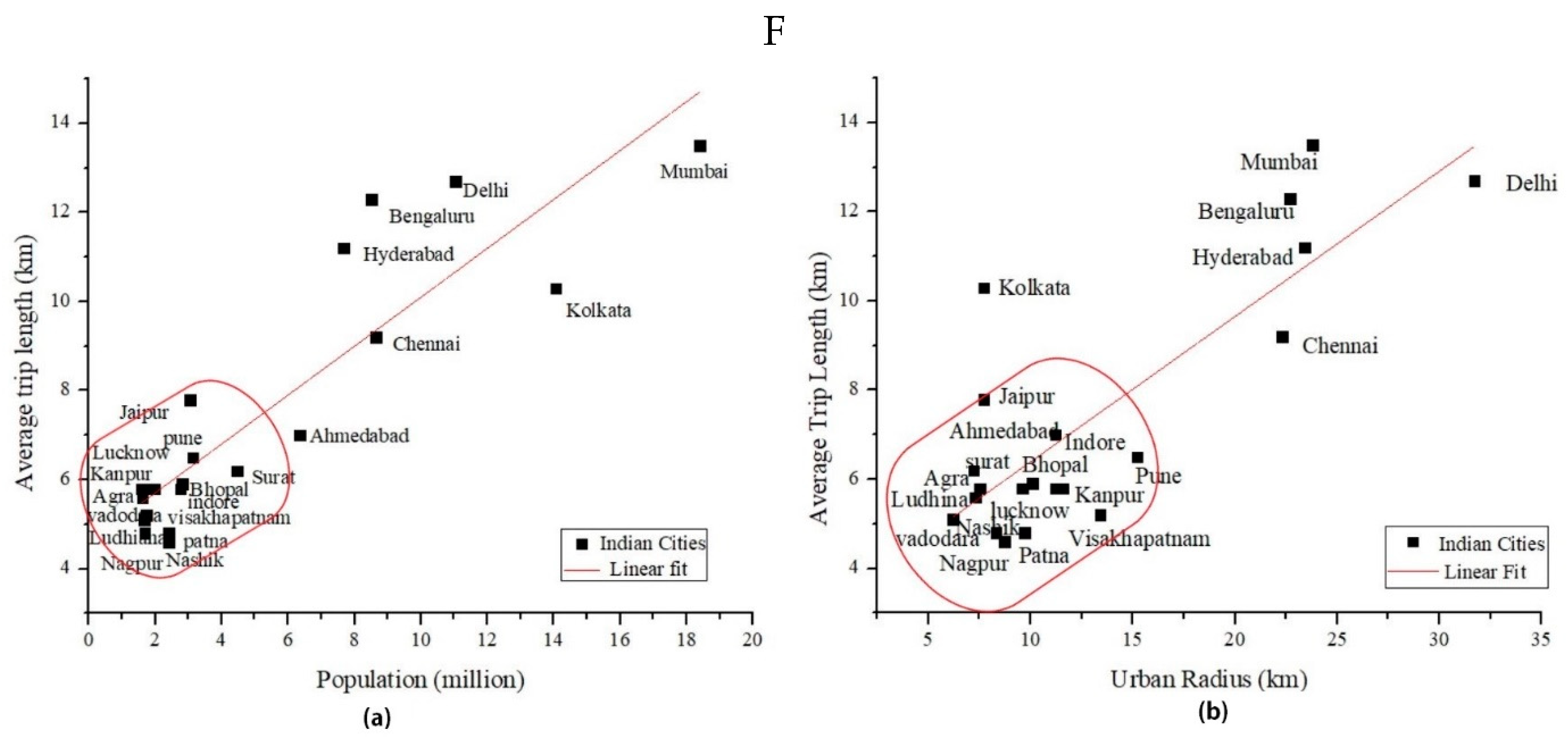
Previously in India, studies conducted at city level focused on accessibility assessment to jobs through public transport. These studies are mostly conducted in tier-1 cities, or cities with a population over 3 million as per the 2011 census, such as Mumbai, Delhi, Kolkata, Chennai, Hyderabad, Bengaluru, Ahmedabad, Surat, and Pune. Only a limited number of studies have focused on issues of access by walking to public transit at the city level to educational facilities [70,76]. However, these studies were limited for tier-2 cities. Most of the Indian tier-2 cities with a population of 1.5 to 3.0 million have an average trip length of less than 6km and the urban radius (which is determined as population distribution by distance from the center of the city) is within 15 km from the center, as shown in Figure 3a,b [77,78].
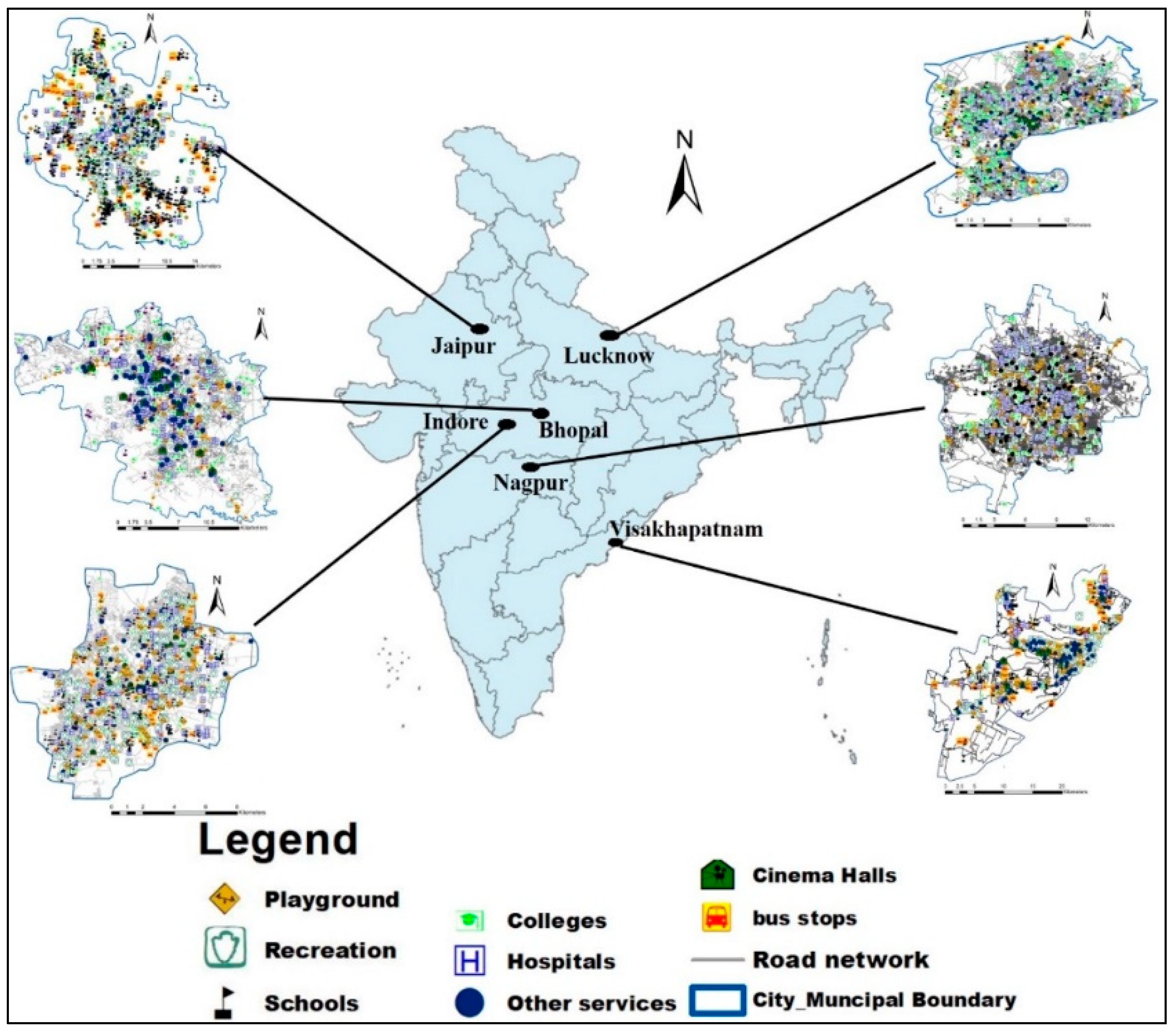
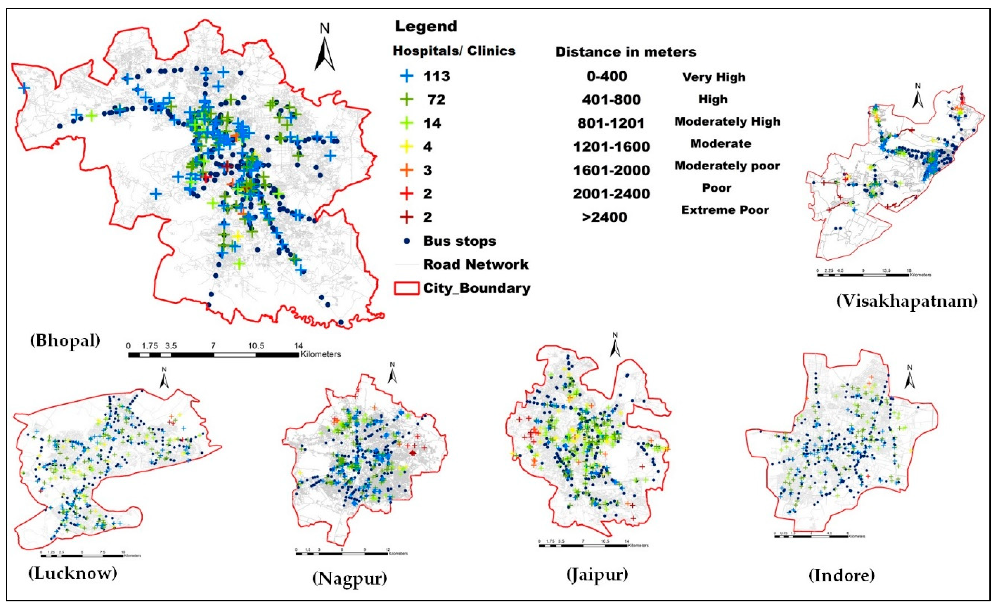
For the current study, large cities with a population of over 3.1 million were ignored, as these cities exhibit unique characteristics in comparison with the million-plus cities in India. Moreover, limited studies were conducted for the shortlisted cities, on the accessibility of PT (PT in this study considers only bus stops). Therefore, confining this scope, the present study attempts to assess the accessibility to various ASFs from bus stops at the city level. All these cities were shortlisted based on population size and presence of a public transportation facility in the city as shown in Figure 4. For this paper, out of the 11 shortlisted cities, only 6 were considered (Visakhapatnam, Nagpur, Bhopal, Jaipur, Lucknow, and Indore), as shown in Figure 4 with blue colour bar, and they are mapped accordingly in Figure 5.
The average mean distance between bus stops in all the selected six cities was almost below 500 m, as calculated using the average neighborhood tool in ArcGIS 10.5.1. This is the reliable distance between bus stops (<500 m) as per the World Banking Group [64]. The shape of the city is identified from a study wherein it considers dynamic growth, density and development patterns along with the road network [77], and is mentioned in Table 5.
3.2. Data Collection
Secondary and spatial data were collected from various sources, as shown in Table A1 in Appendix A. Data are mapped using OpenStreetMap (OSM) in Google Earth (GE) and imported into ArcGIS 10.5.1 for analysis, as shown in Figure 6. For built-up area, the Landsat 8 image of datum WGS84 was used shown in Table 6. Bands 4, 3 and 2 were combined to create true-colour composite images. For analyzing the land cover, supervised classification was performed by a pixel-based supervised classifier, in which other land covers such as forest, agriculture, and water bodies were excluded from this study and only built-up area was delineated and used. The data from OSM in GE were overlapped with built-up area, as accessibility is crucial for identifying geo-located features and labels. The combination of earth observations with OSM features is a tool for large maps and offers significant opportunities for the creation of ideas [81].
4. Data Analysis
The analysis aims at developing a step by step assessment method. Initially, the quality and accuracy of data were checked by testing them for one city and secondly data processing and mapping were carried out by measuring accessibility by Euclidean and network distance for various indicators in six cities. From the literature, network connectivity, network density and detour index were calculated using the relevant equations. Lastly, the cumulative accessibility score (index) was calculated by combining the relevant indicators through the process of normalization.
4.1. Data Quality and Accuracy
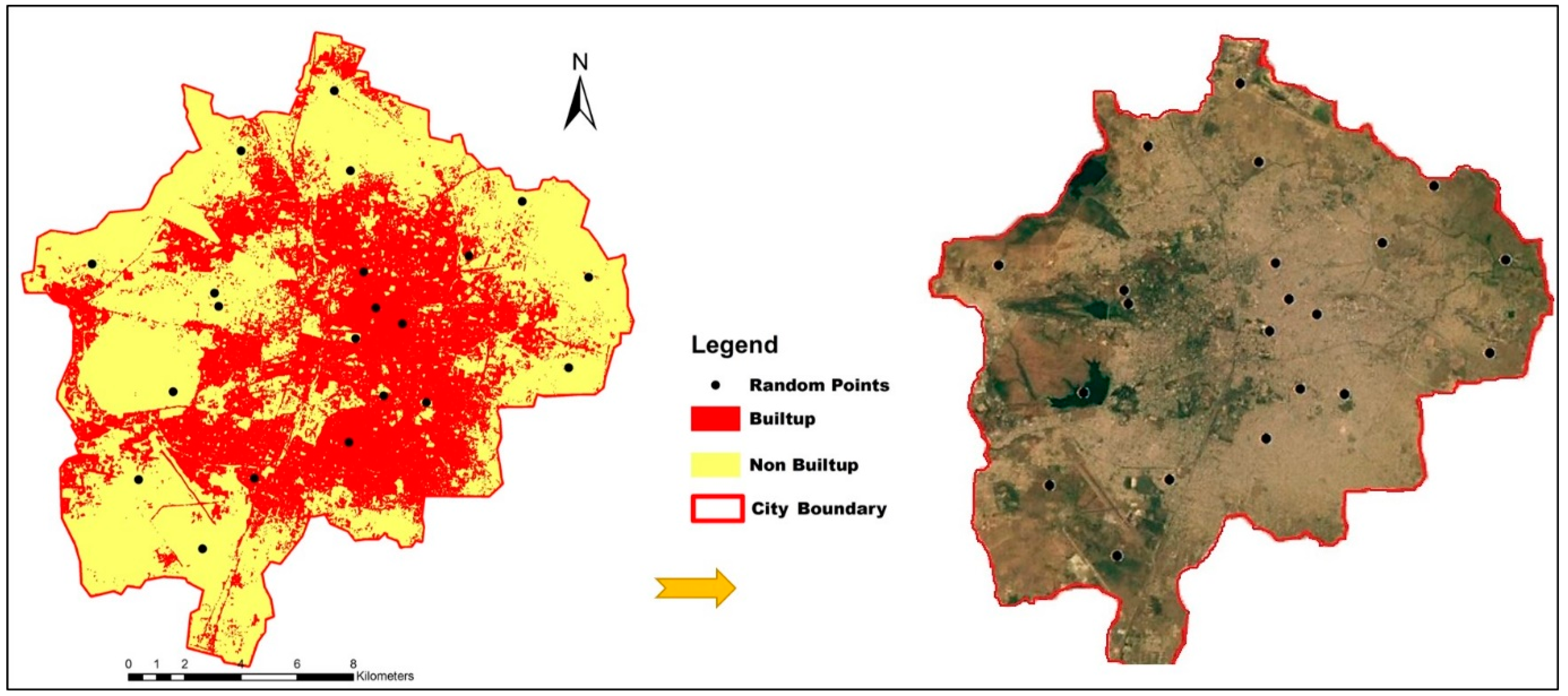
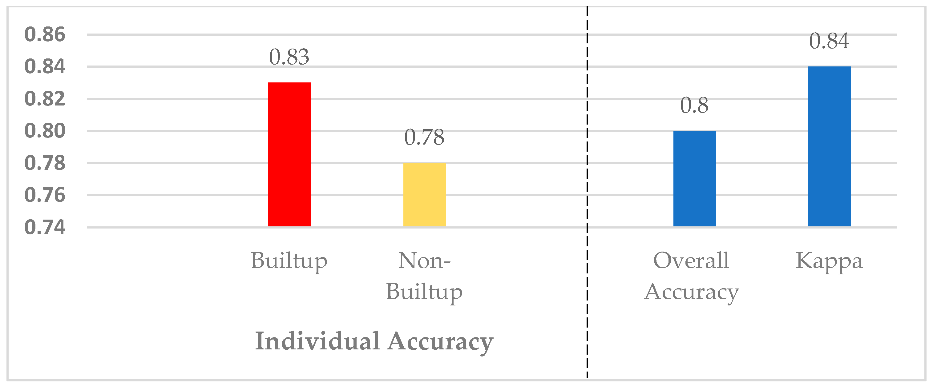
Research quality may be defined by the reliability and credibility of information and data. Precision and error-free data are the key characteristics of data accuracy [82]. This study uses built-up area extracted from Landsat 8. Initially, the study examines the accuracy assessment of land cover classification using GE with Nagpur city for the year 2018. The supervised classification was used to classify the image of Nagpur city for projected coordinate system of “WGS_1984_UTM_Zone_44N”. Under land cover categories, built-up and non-built-up were classified (refer to Figure A1 in Appendix A). After classification of land cover types, 20 random points were generated in ArcGIS 10.5.1 and random points were converted to KML for opening in GE. Each random point’s value was verified from GE for accuracy assessment. GE was used to measure the number of correctly classified ground truth pixels, as shown in Equations (1) and (2). Since GE has a high resolution, it is an important source of information, especially in an urban area where the pattern of land cover is a complex mosaic of different land uses [83]. The source of data is open, and therefore, a manual visual interpretation approach on the GE interface was carried out for 26 November 2018. The result shows that the overall accuracy of land cover for 2018 is 80% and Kappa (K) is 0.84, which is acceptable in both overall accuracy and Kappa accuracy (Refer Figure A2 in Appendix A).
Secondly, data acquired from various government sources were mapped using OSM in GE. To check accuracy, ground truthing was conducted randomly in the city of Nagpur for three areas in the year 2018 with a buffer ring of 800 m from the main bus stop in each area, as shown in Figure A3 in Appendix A. In general, the Kappa coefficient is performed to understand the plots’ mismatch and is mostly used in land cover classification, which was done initially. In this case, the data point for schools, playgrounds and recreation etc. was vpresumed in OSM, and ground truthing was done by directly visiting the site and checking the existence of ASFs by using GPS coordinates. Mismatch is mainly seen in playground and recreational areas, where it is verified by reaching out to the precise location. Where a few locations are rarely inconsistent, and when one or two locations are found, these are drawn into other services in the evaluation process. The results are shown in Table A2 in Appendix A for the individual area, and the overall accuracy within all the areas is shown in Figure A4 in Appendix A. The accuracy results confirm that the overall accuracy is above 90.0% and Kappa (K) is above 0.85 in all the cases. Studies showed that accuracy higher than 75% is reliable and acceptable [83]. Previously, a study in Nagpur conducted on validation georeferenced Google Earth imagery (GEI) with ground truthing for recreation and playgrounds had a confirmed 95% accuracy, with a kappa value of 0.93 (i.e., 93%), which followed the same method [84]. Other studies in Indian cities compared Landsat 8 images with GE and OSM data, resulting in 87 percent total accuracy in large scale land utilization [85]. This shows that OSM data in Indian cities are sufficiently reliable for analysis.
4.2. Data Processing
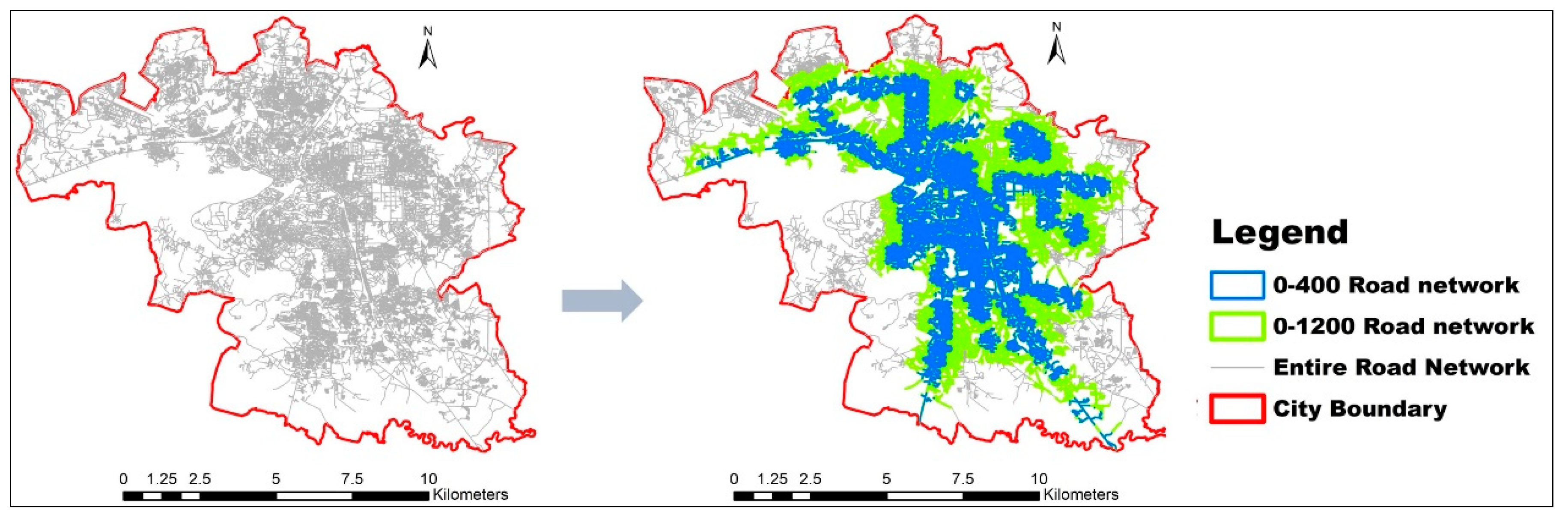
Initially, the distance from bus stops to the grids is considered and as per various levels of accessibility indices distance, colour-coding is assigned to the grid. Furthermore, this grid is overlapped with the existing built-up area (This is done to categorize levels of accessibility as per distance), as shown in Figure 7, for the city of Bhopal. A similar process was adopted for the other five cities and the percentage of built-up area is observed in Figure 8. A high association of built-up area to PT will help in reducing travel distance and vice versa [4].
4.3. Measuring Accessibility
Two measures of accessibility are selected (i) Euclidean distance and (ii) network distance—both of these measures have a single component. The first measure is proximity distance, while the latter one is actual distance calculated using the existing ground network. Furthermore, network connectivity, density and detour index are analyzed accordingly.
4.3.1. Euclidean Distance Measure Using a Near Tool
Near-tool is used to calculate the distance in ArcGIS 10.5.1. This tool calculates the distance from each point in the class to the next point in a different feature class (ESRI, 2018). Here, the origins are ASFs and destinations are bus stops. The process is based on the Pythagoras theorem Equation (3).
from Equation (3) a = shortest distance between two points (ASF and bus stop)
x1, y1 are the geographic coordinates of the centroid of each ASFs.
x2, y2 are the geographic coordinates of each bus stop.
Euclidean distance accessibility levels are considered up to 2400 m; above this range of distance, bus stop facilities are considered not available. Initially, the distance from the bus stop is measured to the nearest ASFs. For example, in Figure 9, for hospitals and clinics, the distance is measured from the bus stops. Depending on the range of distance, every hospital and clinic will be designated a color and symbol, intersecting the built-up area with the same colour (Figure 7). Similarly, this process is repeated for the remaining sectors of ASFs in all the six cities. As all the ASFs are represented as a point, moreover for recreation and playgrounds the points are considered at the entrance. Here, the ASFs percentage for very high access range (0–400 m) is shown in Table 7, and the total percentage of ASFs combined (average of recreational places, playgrounds, cinema halls, other services, hospitals and clinics, schools and colleges), noted for Euclidean distance for entire range (0–2400 m) in all the six cities, is shown Table 8.
4.3.2. Network Distance
A network layer was first created in ArcGIS 10.5.1. Using the Network Analyst tool, the origins and destinations are determined. The shortest part to reach the bus stops from ASFs is measured in network analysts. The ArcGIS network analyst tool makes use of Dijkstra’s algorithm to find the shortest path between two points along a network. One-way restrictions are ignored, while U-turns are permitted at junctions because no mode was considered, and no barriers were assumed restricting movement along the roads. The ArcGIS 10.5.1 Network Analyst allows all points that are used in the analysis to snap to the nearest orthogonal position and measure the distance. Different colour codes are given based on distances from 400 to 2400 m.
In this case, the OSM’s network data are more accurate and up-to-date relative to the available urban development plans in selected cities. A topology analysis tool in ArcGIS 10.5.1 is used for necessary inspections and modifications to OSM’s road system. Accordingly, it modified pseudo nodes and dangles errors.
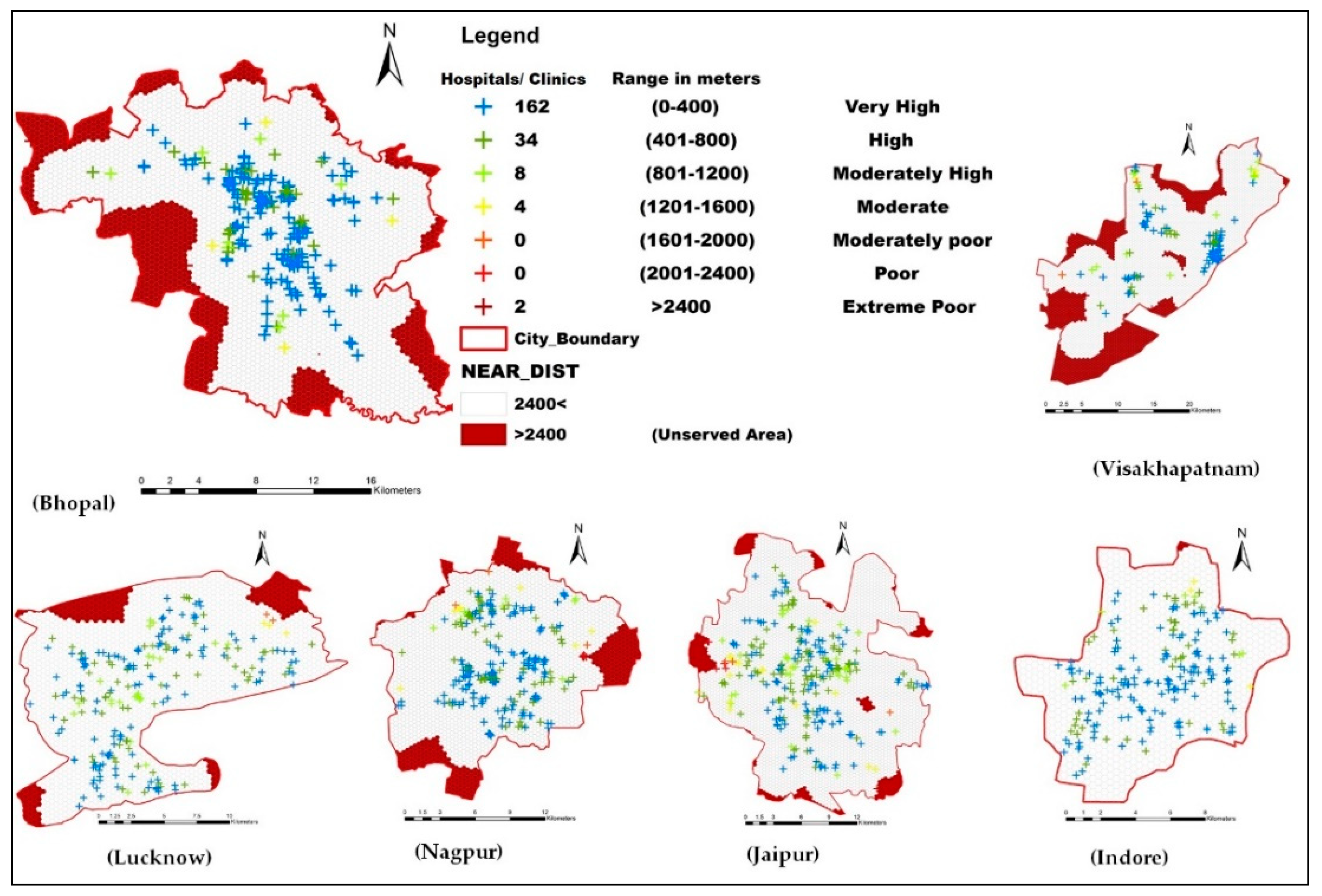
The distance was calculated from the closest bus stop to ASFs. Here, for example, hospitals and clinics are mapped by considering the entire network distance to a bus stop and assigned a different colour according to the range of distance, as shown in Figure 10. Similarly, distance is measured for the remaining sectors of ASFs in all the six cities. Here, the ASFs percentage for very high access range is shown in Table 9, and the total percentage of ASFs combined is noted for network distance in all the six cities, as shown in Table 10.
In all the cases of Table 8 and Table 10 for Euclidean and network distance, it is observed that over 68% of ASFs are in the moderately high level of accessibility. Thus, network connectivity and density have been examined for the very high accessibility range 0–400 m and moderate-high range 0–1200 m. The entire city network is examined to identify the network condition affecting the percentage of accessibility.
4.4. Network Connectivity and Density
“The connectivity of a network may be defined as the degree of completeness of the links between nodes” [86]. The greater the degree of connectivity within a road network, the more efficient that system is. While examining any road network, one should investigate connectivity associations with links and nodes. Studies have shown that in response to the addition of any new links in the future, or the improvement of the existing links, changes to the structure of a road network will have a greater impact on physical accessibility. If there are a greater number of links connecting nodes, the chances of having the shortest part influences accessibility in a better way [51]. Considering the same criteria, this study uses a beta index to identify which city has an efficient ratio of links to nodes that influences connections between ASFs and bus stops.
The beta index is expressed as shown in Equation (4), where E is the total number of edges and V is the total number of vertices in the network. A highly connected transport network will have a high value, and a simple network will have a low value [50]. As the number of edges (links) increases, the connectivity between the vertices (nodes) rises, and the beta index changes progressively.
where E = Edges, V = Vertices.
Here, in this study, the entire city’s edges and vertices are calculated for distance range of 0–400 m and 0–1200 m from bus stops to the network directly. This is done using buffer tool in ArcGIS 10.5.1. The ratio of total edges to vertices is calculated in the segments of 0–400 m and 0–1200 m and likewise for the entire city within the flat buffer area. The edges to vertices ratio is calculated overall and not at a single junction, as shown in Figure 11, for Bhopal city, and similar analysis is done for other cities as summarized in Table 11.
Similarly, network density is calculated using Equation (5), for all six cities at various levels, as shown in Figure 12. The density of the road network is the total amount of the road network length to the size of the city multiplied by 100 [87,88]. Here, in this case, the total area in the range of 0–400 m, 0–1200 m and the entire city is calculated accordingly, the road lengths are considered and summed.
where D is the the density of the roads network, ∑L is the summation of the total road’s length, and S is the city area (square kilometers).
4.5. Detour Index
The detour index (DI) is a measure of the amount of detour from the shortest route that connects two points, as shown in Equation (6) [89]. The detour index sums up a relation in a single index between network distance and the Euclidean distance. A higher detour index value means that the network distance deviates to a greater extent from the Euclidean distance and vice versa.
(Here, road network distance of all ASFs to PT/Euclidean distance of all ASFs to PT and then multiplying by 100).
4.6. Normalization and Benchmarking for Comparing Cities
Different units of indicator values such as distances, density percentages have been standardized as a common unit in a standard form. Such normalization is necessary to prevent inconsistencies, as one indicator value may be between 0 and 200 and other indicator value may be within the range of 0 and 50. In this study, vector normalization is used based on Equation (7). The different dimensions of attributes are transformed into non-dimensional attributes that allow comparisons between criteria [90]. Since different criteria are generally measured in different units, thus it brings into a single unit ranging from 0–1. It creates an evaluation matrix consisting of m alternatives and n criteria, with the intersection of each alternative and criteria given as Xij, therefore, have a matrix (Xij)m × n [91]. Generally, this normalization technique is used in studies of Multiple-Criteria Decision Analysis such as TOPSIS, AHP [92,93]
The matrix (Xij)m × n is normalized to form R = (rij)m × n
where i = 1, 2, ……, m and j = 1, 2, …, n.
Benchmarking is used to compare the level of performance of the indicators that are used to measure the performance of cities. This is further comparable between countries and allows verification for others in the targeted level [21,93].
Sensitivity Analysis
Sensitivity analysis is a study of how uncertainty in the output of a mathematical method or system (numeric or otherwise) can be divided and assigned to unique sources of uncertainty in its inputs. Sensitivity analysis tests the robustness of the results, i.e., whether the results produced using a certain method are accurate and identical to those obtained by other methods, not skewed or affected by a certain phase involved in the above normalization process [94]. Here, this analysis is performed only to check whether the ranks produced by both normalization methods are similar. Although in this study the vector method is adopted to rescale the indicators score, the resultant for all ASFs is also compared with results obtained using another rescaling method (minimum-maximum) of normalization. Here the transformation is based on a range of values Equation (8)
5. Results
The outcomes drawn from the analysis are put into two stages. Initially, in the first stage, the study compares the difference between the Euclidean and network distance for all ASFs from bus stops by evaluating it for all six cities. The first stage includes four assessment criteria—(i) the percentage of ASFs available within the various range of distances 0–400, 401–800 and 801–1200 m, (ii) correlation between Euclidean and network distances for entire city, (iii) mean of Euclidean and network distances for entire city, (iv) difference between Euclidean and network distances within various range of distances for ASFs sector-wise (0–400, 401–800, 801–1200 m). In the second stage, the discussion is carried out by relating the criteria (v) built-up area, network connectivity, network density with the percentage of ASFs in the range of 0–400 m, and the detour index. Finally, (vi) normalization is done by merging the results of the two stages.
- (i)
- The percentage of ASFs available within a various range of distances, 0–400, 401–800 and 801–1200 m
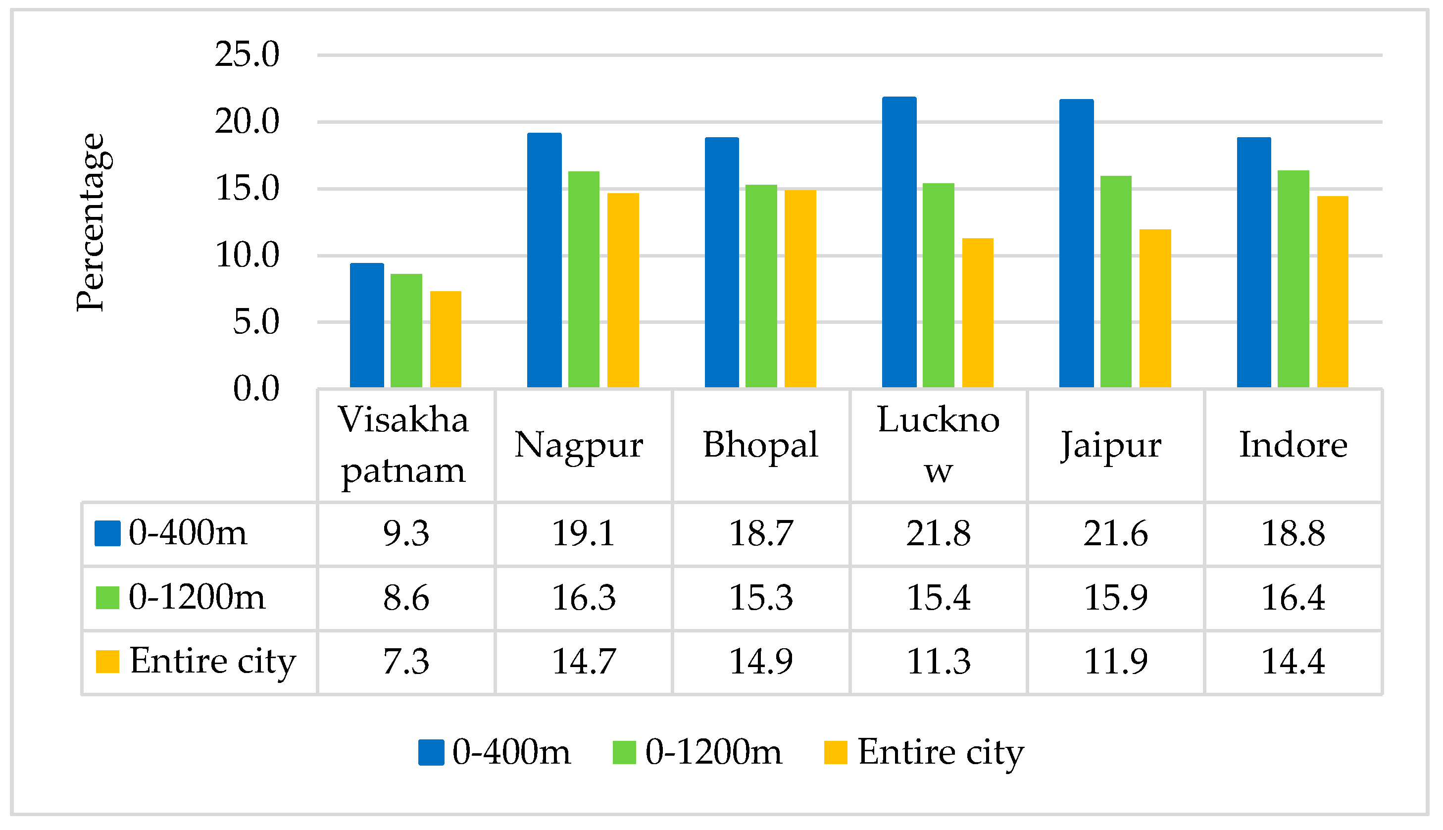
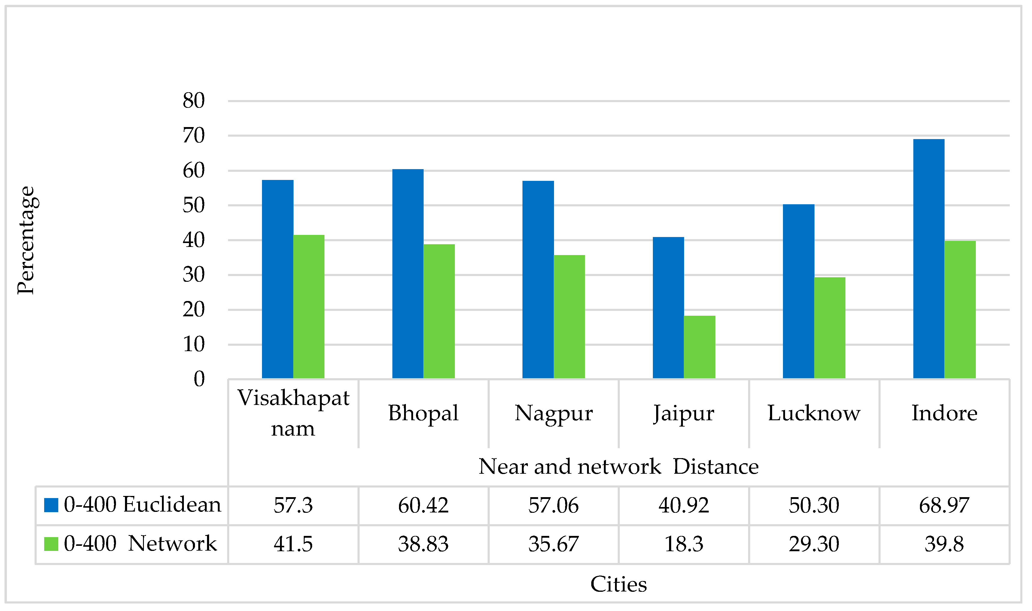
The comparison between Euclidean and network distance (0–400 m) for very high-level ASFs is shown in Figure 14. The result shows 50% to 69% of combined ASFs are easily accessible through Euclidean distance of 0–400 m range, but through network distance, the combined ASFs percentage for the same range is nearly half of the Euclidean distance in all the six cities. This observation suggests the presence of local natural and humanmade physical barriers; undesirable location of bus stops and bus routes; and network issues, which tend to increase the distance and lower the accessibility to ASFs.
The percentage of ASFs across the identified individual sectors (example hospital and clinics) is observed by comparing Table 7 with Table 9 for the (0–400 m) very high accessible range. In Visakhapatnam city, for hospitals and clinics, the low difference (9.77%) between Euclidean and network distance indicates high accessibility by using the network. In Nagpur city, for playgrounds the high difference (26.31%) between Euclidean and network distance indicates low accessibility by using network in 0–400 m range. For other services, the percentage difference is 44.44% between Euclidean and network at a 0–400 m range which is high when compared to other sectors in Bhopal city.
The results from Table 8 and Table 10 are compared for the range of 0–400 m combined ASFs. It is observed that Indore city is having the highest percentage by Euclidean distance while Jaipur city is having the lowest. This scenario is entirely different in case of network distance, where almost 30% of combined ASFs are inaccessible in the case of Indore city as shown in Figure 14. It is observed that almost 70% of combined ASFs are accessible within 1200 m range of network in all the cities (Table 10). Above all, hospitals and clinics, other services have high accessibility to bus stops in all the cities in the range of 0–400 m compared to the rest of the ASFs through Euclidean as well as network distance.
- (ii)
- Correlation between Euclidean and network distance
The overall Euclidean and network distance correlation is performed for entire ASFs in all the cities using Pearson’s correlation method to find the relationship. First, evidence shows high correlation at very similar rates in all the cities except Indore city as shown in Table A3 in Appendix A. It has been verified at a 0.01 (2-tailed) significant level. Since, the R2 variance only shows the relationship between Euclidean and network distance, hence descriptive statistics analysis is performed to identify the difference between Euclidean and network distances in meters.
- (iii)
- Mean of Euclidean and network distance
Descriptive statistics are performed in the Social Sciences Statistical Package (SPSS 16.0) for the selected six cities, and the combined mean average of ASFs for every city is given in Table 12. It provides scope for identifying the average difference in the city. The difference is very less in Nagpur city with 212.4m compared to other cities while it was higher in Jaipur city.
- (iv)
- Difference between Euclidean and network distances within various range of distances for ASFs sector-wise (0–400, 401–800, 801–1200 m)
The correlation, mean difference between Euclidean and network distance for ASFs were observed, as they influence the identification of network connections in the city for reaching bus stops. While considering the entire city, high correlations were found among all the cities as shown in Table 11. Now, by considering it for different threshold ranges 0–400, 401–800, 801–1200 m for ASFs by sector wise in all the six cities, as shown in Table A4 in Appendix A. For the range 0-400 m, the observed correlation is 0.02 to 0.86, p < 0.001, for 401–800 it is 0.09 to 0.79, p < 0.001; and for 801–1200 m it is 0.25 to 0.91, p < 0.001. These values show significant correlations when comparing all sectors of ASFs, and the range varies as high as R2 = 0.91 and as low as R2 = 0.02 in all the six cities. Even in this case, very low correlation is observed in Indore city compared to the other five cities. The average difference between the Euclidean and network distances within each range in all six cities is as high as 50% in each sector for all ASFs. The resultant difference between Euclidean and network distances vary which is very logical as it is based on ground reality.
- (v)
- Relating built-up area, network connectivity and network density with a percentage of AFSs in 0–400 m range:
The relationship between built-up and network connectivity and density is one of the important characteristics for identifying the city’s accessibility [56]. In all six cities, as shown in Figure 15, it is observed that Indore city has the highest built-up area percentage and Visakhapatnam city has the lowest.
Despite less network density and built-up area, Visakhapatnam city has the highest percentage of combined ASFs accessible using network distance from bus stops compared to other five cities. ASFs are accessible using network distance from bus stops. In the case of Jaipur city, even though it has both high network density and better connectivity, as shown in Table 11 but has a low percentage of combined ASFs present in this range which in turn affects accessibility. For Lucknow city, the network density is very high compared to the other five cities.
Visakhapatnam has the lowest detour index for all combined ASFs 0–400 m range of accessibility, as well as for the entire city network, shown in Figure 13. The length of edges within the road network connecting bus stops from ASFs is lower compared to the rest of the cities. While it is upturned in the case of the city of Jaipur, where the edge length is 0–400 m high. In the case of Indore, the detour index is very high, which indicates that the edge length is substantially large in the city connecting bus stops from all combined ASFs compared to rest of the city. It is evident from the findings that a few cities are strong in one dimension and weak in another. To generate consistent results from the different analyses, normalization is done.
- (vi)
- Results of Normalization and Sensitivity analysis
The results of Euclidean and network distances are separately evaluated, and ranks were given to the cities accordingly. The performance was evaluated for the high range of accessibility considering 0–400 m and 0–1200 m for both Euclidean and network distance. For Euclidean distance, the percentage of ASFs accessible (Table 7), built-up area (Figure 8) and the average distance from Appendix A Table A4 were considered and normalized as shown in Table 13 and Table 14. Similarly, for network distance, percentage ASFs accessible (Table 10), network connectivity (Table 11) and the average distance from Appendix A Table A4 were considered and normalized and the results are shown in Table 15 and Table 16.
The results of vector method are compared to the minimum-maximum method for the same indicators as those produced by vector method from Table 13. By rearranging them rank wise, it is observed that scores of both ways vary, but the order of ranks was quite similar, as shown in Table 17. In the vector method, the division of metric units is more precise compared to min-max method.
From the overall results of normalization, it is observed that within 0–400 m and 0–1200 m range of Euclidean distance, Indore city ranks first compared to other cities, as shown in Table 13. However, when considered through the network distance, it is ranked lower. When considered through the network distance, Bhopal city ranks first for network connectivity, and the mean distance to reach ASFs from bus stops is high. In the case of Visakhapatnam city for Euclidean distance, it is poorer because the built-up area is very low in the 0–400 m range. However, when compared by network distance, it ranks second. This is because a large amount of combined ASFs are accessible in this range refer (Table 10) compared to cities of Lucknow, Jaipur, and Indore.
6. Discussions
In this section, the choice of apt indicators to measure accessibility is discussed elaborately. The distance approaches used to evaluate accessibility levels and the ranking of the cities are considered in the following section. Limitations and data constraints for the present study are debated. Overall, how the results can be applied for planning is discussed in detail as follows:
- (i)
- Choice of indicators and methodological concerns
The prime focus is the selection of the most appropriate indicators for defining the accessibility to ASFs from PT. This may depend on several factors, such as the aim of the research or application, the number, and types of data available, the methodological assumptions and the choices (type of distance) made. The evaluation of ASFs is performed as the study aims to understand variation in accessibility in various cities from PT, and particularly which ASFs (such as hospitals and clinics) are more accessible
Using simple distance measures such as Euclidean and network may be most appropriate [38], as they are localized and easy to evaluate ASFs from PT. The choice of built-up area for evaluating the distance in this study becomes crucial for identifying geo-located features and labels. It acts as a background to categorize levels of accessibility as per distance using the grid-based method. In several developed nations, the importance of accessibility instruments in planning practice has increased [41]. But with developing nations, this is still in the commencement stage. However, nowadays, availability of data in OSM has facilitated GIS implementation with the transport module (e.g., ESRI Network Analyst Extension) [39]. The possibility of focusing on city level accessibility using various parameters for spatial assessment in this research became easier in comparing various cities. Hence, the assumption made in the hypothesis was proved, as this study consists of various indicators (based on physical elements such as built up, connectivity and density of ASFs). Although the accessibility of each ASFs differs, grouping as per various accessibility level by evaluating combination of influencing indicators, various scores and ranks are assigned.
- (ii)
- The distance approaches
Euclidean distances are easy to measure in ArcGIS 10.5.1 software and are used in planning applications traditionally [39]. They do not need a network street layer when measuring the distance between ASFs and PT. However, while measuring by network measures, some additional work is normally needed when setting, such as manually snapping points to the network. Euclidean distances do not adequately represent the actual distances. Accessibility can be measured by different methods as discussed in the literature but measuring accessibility by network distance method is an essential tool for any study and at any scale (city, area and neighborhoods) as it focuses on ground reality [48]. This helps to identify the problems at a deeper level, making it easier for both municipal and local authorities to provide recommendations for improvement in preparing a master or regional plan. The network distances used are more accurate and closer to the actual distances. Since they are calculated using road segments, they represent the actual distances that the user has to walk/drive to reach ASFs, which is very well understood from the literature [40]. However, network distances could minimize this effect because, when generating the network in the ArcGIS 10.5.1, ASFs centroids are moved to the nearest element of the street network before the distance is calculated. Although there may be opportunities to use network distance and accessibility points, researchers may prefer Euclidean distance to reduce computation time, when accessibility measures are considered if there is no availability of accurate network data.
- (iii)
- Limitations and data constraints
Data in research play an enormous role while choosing elements for assessment usability, mentioned in the literature analysis, this study uses secondary data. In such cases, there is no choice but to use what one has. However, the quality and accuracy of the data are determined. In all the cities, indicators were measured within the municipal area. Since no spatial data of ASFs outside the city are considered; for this reason, the ’border effect’ may exist and influence the result of Euclidean and network distances which is reported by similar studies of Apparicio [36,37].
- (iv)
- Implications of results in planning
The findings of this study encourage that almost 70% of ASFs are present within 1200 m of bus stops through network distance in all the six cities. However, it is also suggested to increase density of the ASF’s within 400 m in areas nearer to bus stops. This will lead to a higher percentage of ridership by bus. The method of statistical assessment to perform linear regression is easy to understand. The analysis shows a significant correlation for various indicators. In particular, a strong correlation has been found between indicators measured with Euclidean and network distances at the entire overall city level (higher than 0.55, p < 0.001) in all the cities. Significant spatial variations in geographical accessibility were observed across six cities. The analysis demonstrates that regardless of the usage of travel mode and population density, the majority of ASFs in the cities of Lucknow and Jaipur have low access to PT through network distance. Meanwhile, it is high in cities of Visakhapatnam and Indore which is significantly different from results of Euclidean distance. Moreover, the entire data are represented in percentages, which helps in decision making and can be used in further studies that encourage public transportation, NMT infrastructure and high priority bus lanes. The red colour marked on grids and network maps stands out as a challenge, showing the implementation of upcoming bus stops in the future.
There is an uneven distribution of ASFs, where most are concentrated only at the center of the city like for Visakhapatnam. This hampers the availability of the nearest bus stop to a few ASFs at other locations, particularly in newly developed areas. Consideration of built-up area and network density will help to improve the number of additional ASFs within the high access level that are closer to the bus stops and targets in improving the network condition where development would occur in the future. This is provided by the spatial metrics studied in this research.
The location of bus stops used to assess the reliability of bus services have a direct impact on the performance of the transit system and services. However, this study does not evaluate errors in the choice of distance types with aggregation method [36], cost and time [58], and population [38]. Such limited exactitudes could be combined for future studies to automate demand-based bus stop locations which emphasize land use distribution and demand for the service. The results suggest policy and design implications in all the six cities, such that in the initial stage, new regulations of existing guidelines must be implemented at the policy level. The upcoming infrastructure of ASFs must be planned as per consideration by measuring the distance to any nearest PT. Pedestrian planning guidelines in Indian code IRC: 103-2012 should be revised to include distance factor along with the quality of pedestrian infrastructure [95]. The new network should be planned by providing a more significant number of links connecting the nodes. Comparing cities develops a common framework to identify the level of access to each town and issues in those cities [9]. Application of this kind in similar studies will help in comparing cities with benchmarked cities globally and will surely pave a new way. This study focuses on city level assessment, due to its scale/density of activities, it will further hamper the accessibility of the city in future. The ranks are assigned to understand the position of the city by comparing its performance with other cities and to compete to stand as a benchmark and become a target for other cities to achieve and improve PT. Summarizing the nature of ranking in this study shows city of Bhopal, Indore, Visakhapatnam has high rank which stands out as a benchmark, whereas Nagpur, Jaipur, and Lucknow scores low rank for network distance 0–400 m range. In general, the higher the rank, the better it encourages accessibility for ASFs from bus stops.
7. Conclusions
The study adopts a unique approach as it integrates several ASFs and evaluates spatial geographic access to ASFs from bus stops by using both Euclidean and network distance measures in six Indian cities. The study tries to identify the level of accessibility to every ASFs sector-wise connecting the bus stops. Some ASFs from a place of residence may have high accessibility at the neighborhood level but still they do not have a decent bus stop connectivity. Sometimes, people going to the nearest ASFs in a neighborhood may be debated, as they may prefer to move to other ASFs further from home. This study considers the links for the walkable distance between bus stops and ASFs to encourage people to use public transport. The grid map overlapped with the built-up area helps in identifying areas with no transit at all and areas with only a few bus stops. The present work proposes and discusses a set of indicators that can be used in urban planning further. Measures are divided into two major categories: Euclidean and network. First accounts using straight line distance while the second calculates distance by using road network. More precise and accurate results are obtained when using network distance, although using network distance requires more data and analysis (e.g., a network layer). The results obtained by using Euclidean distance overestimate the distance. The results of this research indicate the necessity of land use planning by increasing the density of ASFs in areas close to bus stops, concentrated within 400 m of transit, which in turn leads to a higher percentage of ridership by bus.
In India, current policies on accessibility target on building up new infrastructure, but they do not define how accessibility is achieved in cities and assessment measures required for accessibility planning. In this research, various ASFs are identified based on levels of accessibility and combined with other indicators for ranking. Overall, the percentages at various levels and scores can be considered for further studies and will help researchers and planners in terms of the methodologies used, accepted assumptions, and limitations.
In any context, indicators used for the assessment of the accessibility of ASFs from PT represent very important tool for planning of urban areas in India. They may provide a framework for developing different public transit policies in municipalities and in metropolitan areas (regions, metropolitan areas).
Further research might include the refinement and addition of indicators so that they can further strengthen the integration of various land uses connecting to PT with relevant factors that affect accessibility. A similar methodology can also be adopted in other cities in India for evaluating accessibility. This research explores the possibility of including some of the factors such as slope, elevation and road condition that affects accessibility to reach PT irrespective of shortest distance. These methods can be further applied to other transit such as metros in future, as the choice of origins and destinations may influence interpretation differently for a city.
Author Contributions
Methodology, Pavan Teja Yenisetty; software, Pavan Teja Yenisetty; writing—original draft, Pavan Teja Yenisetty; supervision, Pankaj Bahadure; Writing-review and editing, Pankaj Bahadure. All authors have read and agreed to the published version of the manuscript.
Funding
This research received no external funding.
Acknowledgments
This research is funded by the scholarship awarded to Yenisetty Pavan Teja from Ministry of Human Resource Development (MHRD), Government of India. We also like to thank the editor and two anonymous reviewers for their constructive comments, which helped us to improve the manuscript.
Conflicts of Interest
The authors no conflict of interest.
Appendix A

Table A1.
Data from various government and non-government organizations.
| Sr.No | Data Type | Visakhapatnam | Nagpur | Bhopal | Lucknow | Jaipur | Indore |
|---|---|---|---|---|---|---|---|
| 1 | City base map | Greater Visakhapatnam Municipal Corporation | Nagpur Improvement trust | Bhopal Municipal Corporation | Lucknow Nagar Nigam | Jaipur Nagar Nigam | Indore Municipal corporation |
| 2 | List of hospitals and clinics (GIS shapefile) | Office of the Directorate of Medical Education | Information collected from NMC health office | Information collected from Directorate of Health Services Government of Madhya Pradesh, Smart city cell | Central Government Health scheme list Lucknow. | Department of Medical Health and welfare, Jaipur | Information collected from Directorate of Health Services Government of Madhya Pradesh |
| 3 | List of education Institutes (GIS shapefile) | District Education Officer (Secondary Education) | Information collected from Nagpur divisional education board | Information collected from Madhya Pradesh District School Education Portal, Smart city cell | Basis Education Department (Schoolgis.nic.in) Higher Education Department | Board of Secondary Education, Rajasthan, | Information collected from Madhya Pradesh District School Education Portal |
| 4 | List of parks /gardens and other services (Police station, Post office, community halls) | Information collected from Land use maps (City development plan), smart city maps | |||||
| 5 | Built-up area (GIS shapefile) | Extracted from USGS Landsat Look | |||||
| 6 | Road layer | OpenStreetMap (OSM) | |||||
Figure A1.
Generating random points in ArcMap and opening point in Google Earth.

Figure A2.
Accuracy assessment of land use land cover: 2018.

Figure A3.
Overlapping ASFs on Google Earth; for accuracy assessment in 3 areas by ground truthing.
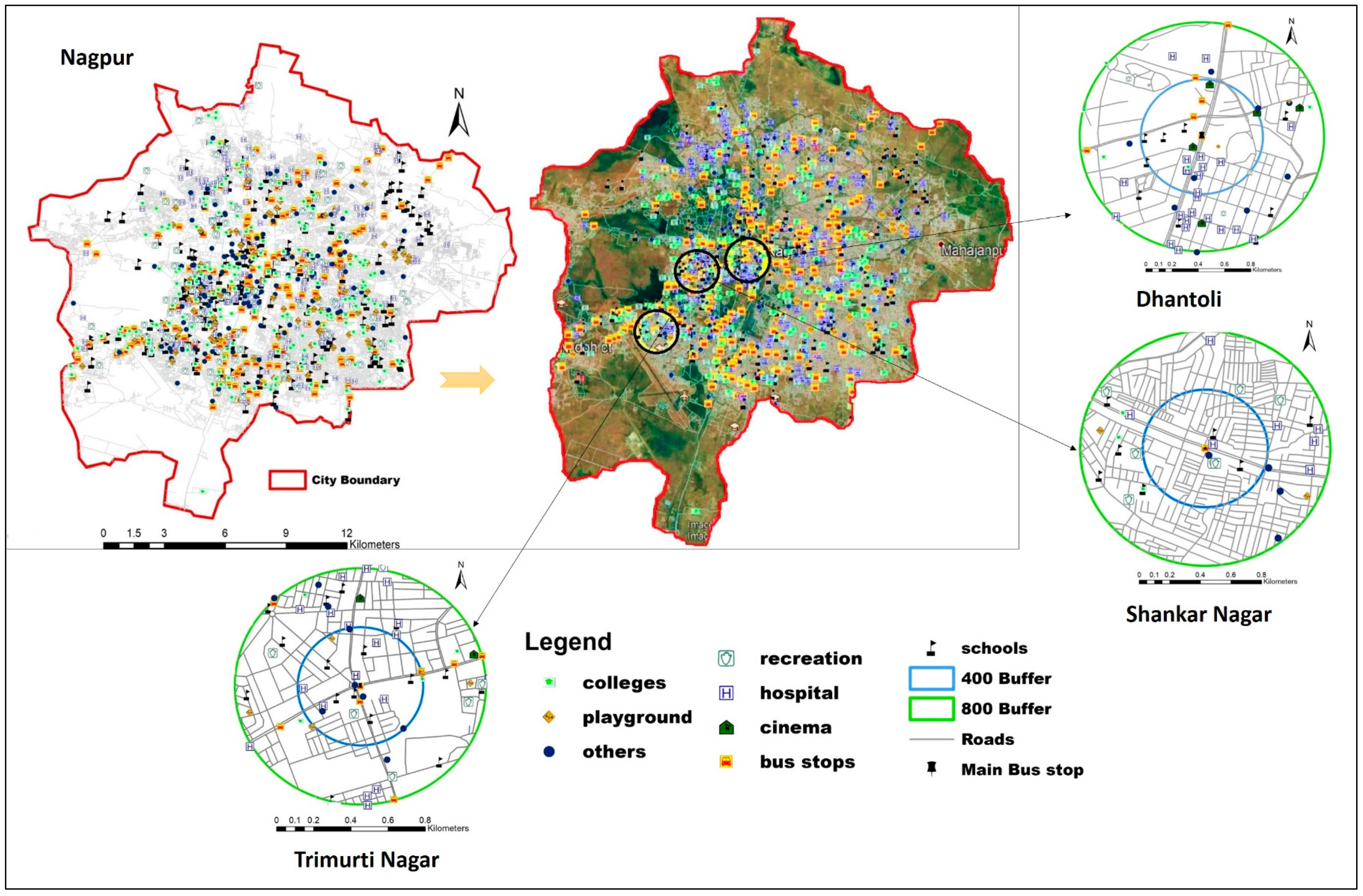
Table A2.
Accuracy assessment and Kappa coefficient for Trimurti Nagar area (ASFs).
| Number of ASFs Mapped in a Particular Area (n) | ASFs | Recreational Places | Playgrounds | Other Services (Post Offices Police Station Community Halls) | Hospital and Clinics | Schools | Colleges | Row Total | Ind. ACC (%) |
|---|---|---|---|---|---|---|---|---|---|
| 5 | Recreational Places | 4 | 1 | 0 | 0 | 0 | 0 | 5 | 80.0 |
| 4 | Playgrounds | 0 | 4 | 0 | 0 | 0 | 0 | 4 | 100.0 |
| 8 | Other services (Post offices Police station Community halls | 0 | 0 | 8 | 0 | 0 | 0 | 8 | 100.0 |
| 14 | Hospitals and clinics | 0 | 0 | 1 | 13 | 0 | 0 | 14 | 92.9 |
| 16 | Schools | 0 | 0 | 0 | 0 | 16 | 0 | 16 | 100.0 |
| 4 | colleges | 0 | 0 | 0 | 0 | 0 | 4 | 4 | 100.0 |
| Total | 4 | 5 | 9 | 13 | 16 | 4 | 51 | 95.5 | |
| (%) | 100.0 | 80.0 | 88.9 | 100.0 | 100.0 | 100.0 | 94.8 | ||
| Overall accuracy | 0.961 | 96.1 | |||||||
| Kappa | 0.92 | 92.6 |
Figure A4.
Overall accuracy assessment and Kappa coefficient results for 3 areas.
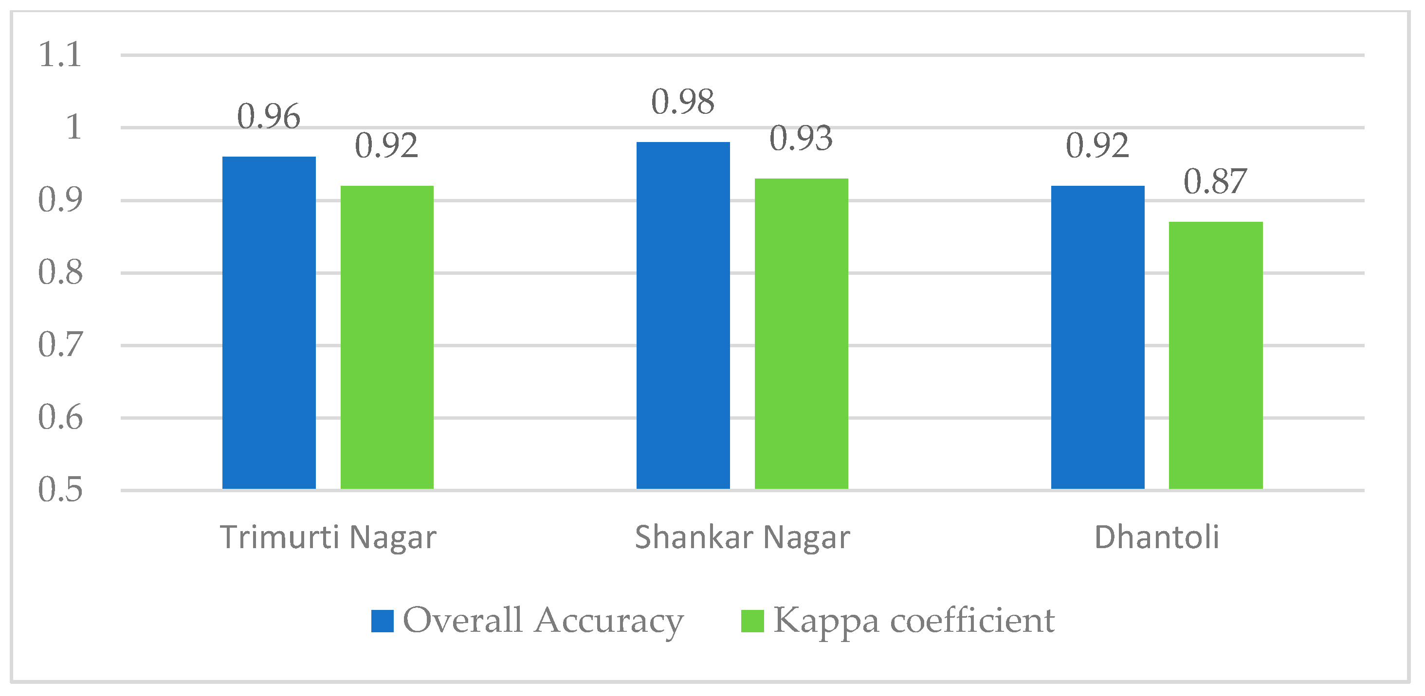
Table A3.
Correlation for overall city Euclidean and network distance.
| ASFs | Visakhapatnam | Nagpur | Bhopal | Lucknow | Jaipur | Indore | ||||||
|---|---|---|---|---|---|---|---|---|---|---|---|---|
| R2 | p-Value | R2 | p-Value | R2 | p-Value | R2 | p-Value | R2 | p-Value | R2 | p-Value | |
| Recreational Places | 0.87 | <0.0001 | 0.8 | <0.0001 | 0.78 | <0.0001 | 0.88 | <0.0001 | 0.87 | <0.0001 | 0.55 | <0.0001 |
| Playgrounds | 0.72 | <0.0001 | 0.84 | <0.0001 | 0.92 | <0.0001 | 0.74 | <0.0001 | 0.81 | <0.0001 | 0.53 | <0.0001 |
| Cinema Halls | 0.9 | <0.0001 | 0.84 | <0.0001 | 0.96 | <0.0001 | 0.86 | <0.0001 | 0.7 | <0.0001 | 0.54 | <0.0001 |
| Other services (Post offices Police station Community halls | 0.74 | <0.0001 | 0.92 | <0.0001 | 0.86 | <0.0001 | 0.78 | <0.0001 | 0.76 | <0.0001 | 0.57 | <0.0001 |
| Hospitals and clinics | 0.9 | <0.0001 | 0.83 | <0.0001 | 0.84 | <0.0001 | 0.75 | <0.0001 | 0.8 | <0.0001 | 0.7 | <0.0001 |
| Schools | 0.71 | <0.0001 | 0.87 | <0.0001 | 0.9 | <0.0001 | 0.78 | <0.0001 | 0.73 | <0.0001 | 0.57 | <0.0001 |
| colleges | 0.89 | <0.0001 | 0.91 | <0.0001 | 0.85 | <0.0001 | 0.86 | <0.0001 | 0.87 | <0.0001 | 0.56 | <0.0001 |
Table A4.
Correlation and average distance difference for ASFs sector-wise in all six cities, for ranges (0–400, 401–800, 801–1200 m).
Table A4.
Correlation and average distance difference for ASFs sector-wise in all six cities, for ranges (0–400, 401–800, 801–1200 m).
| Visakhapatnam | Nagpur | Bhopal | |||||||||||
| ASF’s | Distance in Meters | Average Euclidean Distance | Average Network Distance | Difference in Percentage | R2 | Average Euclidean Distance | Average Network Distance | Difference in Percentage | R2 | Average Euclidean Distance | Average Network Distance | Difference in Percentage | R2 |
| Schools | 0–400 | 193.9 | 310.0 | 62.5 | 0.35 | 214.6 | 379.2 | 56.6 | 0.21 | 223.5 | 353.8 | 63.2 | 0.53 |
| 401–800 | 573.4 | 749.8 | 76.5 | 0.48 | 541.6 | 771.8 | 70.2 | 0.25 | 547.2 | 805.7 | 67.9 | 0.39 | |
| 801–1200 | 1013.9 | 1532.9 | 66.1 | 0.50 | 908.4 | 1509.0 | 60.2 | 0.59 | 935.2 | 1226.2 | 76.3 | 0.16 | |
| Colleges | 0–400 | 240.2 | 339.2 | 70.8 | 0.43 | 319.6 | 670.5 | 47.7 | 0.79 | 223.5 | 353.8 | 63.2 | 0.35 |
| 401–800 | 572.2 | 814.2 | 70.3 | 0.69 | 539.3 | 804.8 | 67.0 | 0.18 | 547.2 | 805.7 | 67.9 | 0.10 | |
| 801–1200 | 953.4 | 1181.4 | 80.7 | 0.59 | 949.2 | 1269.6 | 74.8 | 0.15 | 981.0 | 1594.8 | 61.5 | 0.17 | |
| Hospitals and clinics | 0–400 | 181.6 | 275.9 | 65.8 | 0.30 | 216.0 | 332.1 | 65.0 | 0.39 | 194.1 | 317.4 | 61.2 | 0.35 |
| 401–800 | 524.5 | 675.5 | 77.6 | 0.51 | 537.9 | 714.6 | 75.3 | 0.45 | 525.7 | 750.2 | 70.1 | 0.18 | |
| 801–1200 | 992.4 | 1417.1 | 70.0 | 0.40 | 896.5 | 1125.9 | 79.6 | 0.32 | 494.3 | 764.4 | 64.7 | 0.54 | |
| Other services | 0–400 | 196.7 | 297.3 | 66.2 | 0.10 | 211.0 | 331.4 | 63.7 | 0.48 | 199.6 | 363.1 | 55.0 | 0.28 |
| 401–800 | 571.6 | 853.5 | 67.0 | 0.60 | 545.7 | 734.6 | 74.3 | 0.28 | 547.5 | 830.4 | 66.4 | 0.25 | |
| 801–1200 | 984.3 | 2061.9 | 47.7 | 0.19 | 927.6 | 1317.0 | 70.4 | 0.65 | 1084.5 | 1284.3 | 84.4 | 0.11 | |
| Playground | 0–400 | 279.0 | 879.5 | 31.7 | 0.45 | 231.5 | 427.8 | 54.1 | 0.33 | 234.8 | 420.7 | 55.8 | 0.35 |
| 401–800 | 552.7 | 869.5 | 63.6 | 0.28 | 578.7 | 796.4 | 72.7 | 0.47 | 540.7 | 873.1 | 61.9 | 0.76 | |
| 801–1200 | 1085.1 | 1254.7 | 86.5 | 0.79 | 986.5 | 1234.6 | 79.9 | 0.29 | 387.7 | 646.9 | 59.9 | 0.91 | |
| Recreation | 0–400 | 217.1 | 346.2 | 62.7 | 0.24 | 219.5 | 380.5 | 57.7 | 0.35 | 250.7 | 427.9 | 58.6 | 0.43 |
| 401–800 | 525.6 | 680.6 | 77.2 | 0.63 | 541.0 | 814.3 | 66.4 | 0.19 | 765.1 | 1145.2 | 66.8 | 0.14 | |
| 801–1200 | 899.6 | 1210.4 | 74.3 | 0.22 | 927.6 | 1317.0 | 70.4 | 0.25 | 969.6 | 1336.7 | 72.5 | 0.08 | |
| Cinema | 0–400 | 247.3 | 297.2 | 83.2 | 0.86 | 139.1 | 431.3 | 32.3 | 0.36 | 174.6 | 276.1 | 63.2 | 0.56 |
| 538.9 | 758.7 | 71.0 | 0.10 | ||||||||||
| Lucknow | Jaipur | Indore | |||||||||||
| ASF’s | Distance in Meters | Average Euclidean Distance | Average network Distance | Difference in Percentage | R2 | Average Euclidean Distance | Average Network Distance | Difference in Percentage | R2 | Average Euclidean Distance | Average Network Distance | Difference in Percentage | R2 |
| Schools | 0–400 | 226.7 | 476.7 | 47.6 | 0.12 | 257.5 | 554.7 | 46.4 | 0.14 | 233.4 | 433.3 | 53.9 | 0.3 |
| 401–800 | 590.6 | 880.0 | 67.1 | 0.12 | 579.4 | 875.2 | 66.2 | 0.29 | 545.9 | 864.2 | 63.2 | 0.1 | |
| 801–1200 | 927.0 | 1242.0 | 74.6 | 0.21 | 958.1 | 1310.0 | 73.1 | 0.39 | 967.9 | 1331.7 | 72.7 | 0.3 | |
| Colleges | 0–400 | 227.0 | 405.0 | 56.0 | 0.29 | 224.3 | 434.3 | 51.6 | 0.14 | 204.8 | 416.9 | 49.1 | 0.1 |
| 401–800 | 574.0 | 813.0 | 70.6 | 0.21 | 582.4 | 940.7 | 61.9 | 0.32 | 534.8 | 781.4 | 68.4 | 0.1 | |
| 801–1200 | 932.0 | 1243.0 | 75.0 | 0.20 | 981.5 | 1367.9 | 71.8 | 0.36 | 869.82 | 599.133 | 61.7 | 0.1 | |
| Hospitals and clinics | 0–400 | 200.0 | 394.0 | 50.8 | 0.22 | 235.2 | 511.9 | 45.9 | 0.50 | 195.7 | 388.9 | 50.3 | 0.1 |
| 401–800 | 554.0 | 808.0 | 68.6 | 0.40 | 579.1 | 813.0 | 71.2 | 0.40 | 544.4 | 765.3 | 71.1 | 0.1 | |
| 801–1200 | 939.0 | 1226.0 | 76.6 | 0.25 | 998.8 | 1360.8 | 73.4 | 0.15 | 964.1 | 1274.0 | 75.7 | 0.5 | |
| Other services | 0–400 | 208.0 | 390.0 | 53.3 | 0.29 | 208.0 | 438.1 | 47.5 | 0.18 | 138.9 | 350.4 | 39.6 | 0.0 |
| 401–800 | 571.0 | 798.0 | 71.6 | 0.36 | 579.0 | 808.0 | 71.7 | 0.35 | 567.9 | 764.9 | 74.3 | 0.6 | |
| 801–1200 | 897.0 | 1106.0 | 81.1 | 0.41 | 990.0 | 1452.0 | 68.2 | 0.25 | 1038.5 | 1454.2 | 71.4 | 0.6 | |
| Playground | 0–400 | 267.0 | 513.0 | 52.0 | 0.41 | 266.4 | 522.5 | 51.0 | 0.15 | 210.1 | 455.2 | 46.2 | 0.2 |
| 401–800 | 641.0 | 949.0 | 67.5 | 0.55 | 575.7 | 896.8 | 64.2 | 0.23 | 524.4 | 760.9 | 68.9 | 0.3 | |
| 801–1200 | 963.0 | 1342.0 | 71.8 | 0.50 | 956.9 | 1334.91 | 71.7 | 0.43 | |||||
| Recreation | 0–400 | 238.0 | 465.0 | 51.2 | 0.19 | 286.6 | 496.4 | 57.7 | 0.25 | 247.5 | 453.0 | 54.6 | 0.1 |
| 401–800 | 576.5 | 864.0 | 66.7 | 0.28 | 570.5 | 1016.5 | 56.1 | 0.24 | 536.6 | 805.1 | 66.7 | 0.3 | |
| 801–1200 | 929.0 | 1302.0 | 71.4 | 0.37 | 957.0 | 1334.2 | 71.7 | 0.59 | 940.9 | 1332.3 | 70.6 | 0.8 | |
| Cinema | 0–400 | 174.0 | 315.0 | 55.2 | 0.60 | 210.8 | 417.6 | 50.5 | 0.40 | 166.3 | 362.5 | 45.9 | 0.3 |
| 401–800 | 447.0 | 749.0 | 59.7 | 0.39 | 571.5 | 731.1 | 78.2 | 0.50 | 540.8 | 838.2 | 64.5 | 0.4 | |
| 801–1200 | 1007.0 | 1313.0 | 76.7 | 0.71 | 846.9 | 1002.4 | 84.5 | 0.32 | |||||
References
- Saghapour, T.; Moridpour, S.; Thompson, R.G. Measuring cycling accessibility in metropolitan areas. Int. J. Sustain. Transp. 2017, 11, 381–394. [Google Scholar] [CrossRef]
- United Nations Human Settlements Programme Planning and Design for Sustainable Urban Mobility. Nairobi, Kenya. 2013. Available online: https://unhabitat.org/planning-and-design-for-sustainable-urban-mobility-global-report-on-human-settlements-2013 (accessed on 9 January 2019).
- Le Clercq, F.; Bertolini, L. Achieving Sustainable Accessibility: An Evaluation of Policy Measures the Amsterdam in Area. Built Environ. 2003, 29, 36–47. [Google Scholar] [CrossRef]
- Bok, J.; Kwon, Y. Comparable measures of accessibility to public transport using the general transit feed specification. Sustainability 2016, 8, 224. [Google Scholar] [CrossRef] [Green Version]
- Saghapour, T.; Moridpour, S.; Thompson, R.G. Public transport accessibility in metropolitan areas: A new approach incorporating population densityTayebeh saghapour, Sara Moridpour, Russell G. Thompson. J. Transp. Geogr. 2016, 8, 273–274. [Google Scholar] [CrossRef]
- Duncan, D.T.; Aldstadt, J.; Whalen, J.; Melly, S.J. Validation of Walk Score ® for Estimating Neighborhood Walkability: An Analysis of Four US Metropolitan Areas. Int. J. Environ. Res. Public Health 2014, 8, 4160–4179. [Google Scholar] [CrossRef] [PubMed]
- Lo, R.H. Walkability: What is it? J. Urban 2009, 2, 145–166. [Google Scholar] [CrossRef]
- Chhibber, V. Road Transport Year Book. New Delhi. 2012. Available online: https://morth.nic.in/sites/default/files/Road_Transport_Year_Book_2012_13.pdf (accessed on 9 October 2018).
- Rode, P.; Floater, G.; Thomopoulos, N.; Docherty, J.; Schwinger, P.; Mahendra, A.; Fang, W.; Cities, L.S.E.; Friedel, B.; Gomes, A.; et al. Accessibility in Cities: Transport and Urban Form. LSE Cities Pap. 2014, 3, 1–61. [Google Scholar]
- Singal, B. National Urban Transport Policy. New Delhi. 2014. Available online: https://www.urbantransportnews.com/wpcontent/uploads/2018/08/National_Urban_Transport_Policy_2014.pdf (accessed on 9 October 2018).
- Gurtoo, A.; Williams, C. Developing Country Perspectives on Public Service Delivery; Springer: Berlin, Germany, 2015; ISBN 9788132221609. [Google Scholar]
- García-Palomares, J.C.; Gutiérrez, J.; Cardozo, O.D. Walking accessibility to public transport: An analysis based on microdata and GIS. Environ. Plan. B Plan. Des. 2013, 40, 1087–1102. [Google Scholar] [CrossRef]
- Poelman, H.; Dijkstra, L. Measuring Access to Public Transport in European Cities; DG Regional and Urban Policy: Brussels, Belgium, 2015. [Google Scholar]
- Sen, R.; Quercia, D.; Ruiz, C.V. Scalable Urban Data Collection From The Web. In International Conference on Web and Social Media; Association for the Advancement of Artificial Intelligence (www.aaai.org): California, CA, USA, 2016; pp. 1–6. [Google Scholar]
- Kaufmann, T. A Global Ranking of Cities by Accessibility to Services. Available online: https://web.northeastern.edu/nulab/a-global-ranking-of-cities-by-accessibility-to-services/ (accessed on 25 March 2019).
- Zuidgeest, M.; den Bosch, V.; Brussel, M.; Salzberg, A.; Munshi, T.; Gupta, N.; Maarseveen, V. GIS for multi-modal accessibility to jobs for the urban poor in Ahmedabad. Thirteen. WCTR 2013, 1, 1–20. [Google Scholar]
- Kumar, S. Urban transport in India: Issues, challenges, and the way forward. Eur. Transp. Trasp. Eur. 2012, 52, 1–26. [Google Scholar]
- Bahadure, S.; Kotharkar, R. Assessing Sustainability of Mixed Use Neighbourhoods through Residents’ Travel Behaviour and Perception: The Case of Nagpur, India. Sustainability 2015, 7, 12164–12189. [Google Scholar] [CrossRef] [Green Version]
- Singh, V.; Deshpande, P. People Near Transit, Transit Near People. 2019. Available online: https://www.itdp.in/wp-content/uploads/2019/05/People-Near-Transit-Transit-Near-People.pdf (accessed on 7 February 2019).
- Halder, J. Access to Schooling in West Bengal: A Geo—Social Analysis; Sodhganga: Mysore, India, 2012. [Google Scholar]
- Solanki, H.K.; Ahamed, F.; Gupta, S.K.; Nongkynrih, B. Road Transport in Urban India: Its Implications on Health. Indian J. Community Med. Off. Publ. Indian Assoc. Prev. Soc. Med. 2016, 41, 16–22. [Google Scholar]
- Ruiz, M.O.H.; Sharma, A.K. Application of GIS in public health in India: A literature-based review, analysis, and recommendations. Indian J. Public Health 2016, 60, 51–58. [Google Scholar]
- Drahansky, M.; Paridah, M.; Moradbak, A.; Mohamed, A.; Owolabi, F.; abdulwahab taiwo; Asniza, M.; Abdul Khalid, S.H. Measuring Urban Development and City Performance. Intech 2016, i, 13. [Google Scholar]
- Williams, K.; Burton, E.; Mike, J. Achieving Sustainable Urban. Form; Center for Sustainable Development: London, UK, 1986. [Google Scholar]
- Vaidya, C. URBAN ISSUES, REFORMS AND WAY FORWARD IN INDIA; Department of Economic Affairs, Ministry of Finance, Government of India: New Delhi, India, 2009; pp. 1–12.
- Jafari, F.; Ghorbani, R. Urban Density and Social Sustainable Development on Neighborhoods Case Study: Tabriz, Iran. Geography 2013, 3, 457–467. [Google Scholar]
- Banister, D. Sustainable urban development and transport—A Eurovision for 2020. Transp. Rev. 2000, 20, 113–130. [Google Scholar] [CrossRef]
- Litman, T. Measuring People ’s Ability to Reach Desired Goods and Activities; Victoria Transport Policy Institute: Victoria, BC, Canada, 2016. [Google Scholar]
- Saghapour, T.; Moridpour, S.; Thompson, R.G. Measuring Walking Accessibility in Metropolitan Areas. Transp. Res. Rec. J. Transp. Res. Board 2017, 2661, 111–119. [Google Scholar] [CrossRef]
- Chapman, S.; Weir, D. Accessibility Planning Methods October 2008; New Zealand Transport Agency: Wellington, New Zealand, 2008.
- Breheny, M.J. The measurement of spatial opportunity in strategic planning. Reg. Stud. 1978, 12, 463–479. [Google Scholar] [CrossRef]
- Vale, D.S.; Saraiva, M.; Pereira, M. Active accessibility: A review of operational measures of walking and cycling accessibility. J. Transp. Land Use 2015, 1, 1–27. [Google Scholar] [CrossRef]
- Yawson, D.O.; Armah, F.A.; Okae-Anti, D.; Essandoh, P.K.; Afrifa, E.K.A. Enhancing Spatial Data Accessibility in Ghana: Prioritization of Influencing Factors Using AHP. Int. J. Spat. Data Infrastruct. Res. 2011, 6, 290–310. [Google Scholar]
- Chen, Y.Y.; Wei, P.Y.; Lai, J.H.; Feng, G.C.; Li, X.; Gong, Y. An Evaluating Method of Public Transit Accessibility for Urban Areas Based on GIS. Procedia Eng. 2016, 137, 132–140. [Google Scholar]
- Kompil, M.; Jacobs-Crisioni, C.; Dijkstra, L.; Lavalle, C. Mapping accessibility to generic services in Europe: A market-potential based approach. Sustain. Cities Soc. 2019, 47, 101372. [Google Scholar] [CrossRef]
- Apparicio, P.; Abdelmajid, M.; Riva, M.; Shearmur, R. Comparing alternative approaches to measuring the geographical accessibility of urban health services: Distance types and aggregation-error issues. Int. J. Health Geogr. 2008, 7, 1–14. [Google Scholar] [CrossRef] [PubMed] [Green Version]
- Apparicio, P.; Gelb, J.; Dubé, A.S.; Kingham, S.; Gauvin, L.; Robitaille, É. The approaches to measuring the potential spatial access to urban health services revisited: Distance types and aggregation-error issues. Int. J. Health Geogr. 2017, 16, 1–24. [Google Scholar] [CrossRef] [PubMed]
- La Rosa, D. Accessibility to greenspaces: GIS based indicators for sustainable planning in a dense urban context. Ecol. Indic. 2014, 42, 122–134. [Google Scholar] [CrossRef]
- Azzopardi, J. Effect of Distance Measures and Feature Representations on Distance-Based Accessibility Measures; Lund University: Lund, Sweden, 2018. [Google Scholar]
- Spadon, G.; Brandoli, B.; Eler, D.M.; Rodrigues, J.F.J. Detecting multi-scale distance-based inconsistencies in cities through complex-networks. J. Comput. Sci. 2019, 30, 209–222. [Google Scholar] [CrossRef]
- Hull, A.; Silva, C.; Luca, B. Accessibility Instruments for Planning Practice; Cost Office: Bruxelles, Belgium, 2012; pp. 205–237. ISBN 9789892031873. [Google Scholar]
- Pitot, M.; Yigitcanlar, T.; Sipe, N.; Evans, R. Land Use & Public Transport Accessibility Index (LUPTAI) Tool—The development and pilot applicationfor the Gold Coast Author. In ATRF Forum Papers; Griffith Research Online: Queensland, Australia, 2006; pp. 1–18. [Google Scholar]
- Brömmelstroet, M.; Curtis, C.; Larsson, A.; Milakis, D.; Curtis, C.; Larsson, A.; Milakis, D. Strengths and weaknesses of accessibility instruments in planning practice: Technological rules based on experiential workshops. Eur. Plan. Stud. 2016, 24, 1176–1196. [Google Scholar] [CrossRef] [Green Version]
- Munoz, U.H.; Källestål, C. Geographical accessibility and spatial coverage modeling of the primary health care network in the Western Province of Rwanda. Int. J. Health Geogr. 2012, 11, 40. [Google Scholar] [CrossRef] [Green Version]
- Koohsari, M.J.; Owen, N.; Cerin, E.; Giles-corti, B.; Sugiyama, T. Walkability and walking for transport: Characterizing the built environment using space syntax. Int. J. Behav. Nutr. Phys. Act. 2016, 13, 1–9. [Google Scholar] [CrossRef] [Green Version]
- Ha, P.T.H.; van den Bosch, F.; Quang, N.N.; Zuidgeest, M. Urban Form and Accessibility to Jobs. Environ. Urban ASIA 2011, 2, 265–285. [Google Scholar] [CrossRef]
- Knaap, G.; Ewing, R.; Clifton, K. Seeing the Elephant: Multi-Disciplinary Measures of Urban. Sprawl; University of Maryland: College Park, MD, USA, 2005. [Google Scholar]
- Geurs, K.T.; Ritsema van Eck, J. Accessibility measures: Review and applications. Evaluation of accessibility impacts of land-use transportation scenarios, and related social and economic impact. RIVM Rep. 2001, 787, 1–265. [Google Scholar]
- Coppola, P.; Papa, E. Accessibility Planning Tools for Sustainable and Integrated Land Use/Transport (LUT) Development: An Application to Rome. Procedia Soc. Behav. Sci. 2013, 87, 133–146. [Google Scholar] [CrossRef]
- Agampatian, R. Using GIS to Measure Walkability: A Case Study in New York City; Oyal Institute of Technology (KTH): Stockholm, Sweden, 2014. [Google Scholar]
- Rodrigue, J.P.; Comtois, C.; Slack, B. The Geography of Transport Systems; Routledge: New York, NY, USA, 2016; ISBN 9781317210108. [Google Scholar]
- Sahoo, P.; Dash, R.K. Infrastructure development and economic growth in India. J. Asia Pacific Econ. 2009, 14, 351–365. [Google Scholar] [CrossRef]
- Bowyer, D. Measuring Urban Growth, Urban Form and Accessibility as Indicators of Urban Sprawl in Hamilton, New Zealand; Lund University: Lund, Sweden, 2015. [Google Scholar]
- Fan, P.; Xu, L.; Yue, W.; Chen, J. Accessibility of public urban green space in an urban periphery: The case of Shanghai. Landsc. Urban Plan. 2016, 165, 177–192. [Google Scholar] [CrossRef]
- Yi, L. Evaluation of Accessibility to Primary Schools—The Case of Yuhua, Changsha, China; International Institute for Geo-Information Science and Earth Observation: Enschede, The Netherlands, 2004. [Google Scholar]
- Somenahalli, S.V.C.; Taylor, M.A.P. Road Network Accessibility and Socio-economic Disadvantage Across Adelaide Metropolitan Area. Transp. Dev. Econ. 2016, 2, 1–8. [Google Scholar] [CrossRef] [Green Version]
- Bilek, M.; Amireche, L. GIS-Based Prediction of Metro-Line Impact on Accessibility in Public Transport by Modelling Travel Time: A Case Study of North-Western Zone of Algiers, Algeria. J. Remote Sens. GIS 2017, 6, 1000195. [Google Scholar] [CrossRef]
- Järv, O.; Tenkanen, H.; Salonen, M.; Ahas, R.; Toivonen, T. Dynamic cities: Location-based accessibility modelling as a function of time. Appl. Geogr. 2018, 95, 101–110. [Google Scholar] [CrossRef]
- Bhagat, R.B. Urbanisation and Access to Basic Amenities in India. Urban India 2011, 31, 1–14. [Google Scholar]
- Shankaraling, S.K. Urban Planning for Athani Town: A Spatial Approch; Karnatak University: Dharwad, India, 2012; Available online: https://shodhganga.inflibnet.ac.in/bitstream/10603/21354/12/cover%20page.pdf (accessed on 20 June 2020).
- Ramachandran, V. The Status of Health & Education in India Critical Questions in the Nation ’s Development; Unemployed Dalit Youth Empowerment Mission: Delhi, India, 2015. [Google Scholar]
- Buczkowska, S.; Coulombel, N.; Lapparent, M. De Euclidean versus network distance in business location: A probabilistic mixture of hurdle-Poisson models. HALarchives-ouvertes. Ann. Reg. Sci. 2016, 21. [Google Scholar]
- El-geneidy, A.M. Pedestrian Access to Transit: Identifying Redundancies and Gaps Using a Variable Service Area Analysis Pedestrian access to transit: Identifying redundancies and gaps using a variable service area analysis. In Proceedings of the Transportation Research Board 89th Annual Meeting, Washington, DC, USA, 10–14 January 2010. [Google Scholar]
- Armstrong-Wright, A.; Thiriez, S. Bus. Services Reducing Costs, Raising Standards; The International Bank for Reconstruction and Development, The World Bank: Washington, DC, USA, 2003. [Google Scholar]
- Apparicio, P.; Séguin, A.-M.; Naud, D. The Quality of the Urban Environment Around Public Housing Buildings in Montréal: An Objective Approach Based on GIS and Multivariate Statistical Analysis. Soc. Indic. Res. 2008, 86, 355–380. [Google Scholar] [CrossRef]
- Hirsch, J.A.; Moore, K.A.; Evenson, K.R.; Rodriguez, D.A.; Roux, A.V.D. In the Multi-Ethnic Study of Atherosclerosis. Am. J. Prev. Med. 2013, 45, 158–166. [Google Scholar] [CrossRef] [PubMed] [Green Version]
- Thornton, L.E.; Pearce, J.R.; Macdonald, L.; Lamb, K.E.; Ellaway, A. Does the choice of neighbourhood supermarket access measure influence associations with individual-level fruit and vegetable consumption? A case study from Glasgow. Int. J. Health Geogr. 2012, 11, 1–12. [Google Scholar] [CrossRef] [Green Version]
- Kamruzzaman, M.; Yigitcanlar, T.; Yang, J.; Mohamed, M.A. Measures of transport-related social exclusion: A critical review of the literature. Sustainability 2016, 8, 696. [Google Scholar] [CrossRef] [Green Version]
- Wati, K.; Burke, M.; Sipe, A.P.N.; Dodson, A.P.J. Children’s Cycling Trends, Accessibility to and Utilisation of Urban Facilities in Selected Australian Urban Environments. Children’s Cycling for Transport: Status and Determinants. In Proceedings of the 36th Australasian Transport Research Forum, ATRF 2013, Brisbane, QLD, Australia, 2–4 October 2013; Available online: https://espace.library.uq.edu.au/view/UQ:727069 (accessed on 20 June 2020).
- Bahadure, S.; Kotharkar, R. Framework for measuring sustainability of neighbourhoods in Nagpur, India. Build. Environ. 2018, 127, 86–97. [Google Scholar] [CrossRef]
- Wati, K. Transport Related Social Exclusion in Ahmedabad; International Institute for Geo-Information Science and Earth Observation: Enschede, The Netherlands, 2009. [Google Scholar]
- Gol, M. Urban and Regional Development Plans Formulation and Implimentation (URDPFI) Guidelines. Minist. Urban Dev. 2015, I, 447. [Google Scholar]
- Kotharkar, R.; Bahadure, P. Achieving Compact City Form through Density Distribution: Case of Indian Cities. J. Urban. Plan. Dev. 2020, 146, 1–15. [Google Scholar] [CrossRef]
- Wilbur, S.A. Study on Traffic and Transportation Policies and Stratagies in Urban Areas in India. Minist. Urban Dev. 2008, 105–109. [Google Scholar]
- Kotharkar, R.; Bahadure, P.; Sarda, N. Measuring compact urban form: A case of Nagpur city, India. Sustainability 2014, 6, 4246–4272. [Google Scholar] [CrossRef] [Green Version]
- Shah, J. Public Transport Accessibility Levels for Ahmedabad, India. J. Public Transp. 2016, 19, 19–35. [Google Scholar] [CrossRef] [Green Version]
- Kumar, P. Development Oriented Transit in Indian Cities. School of Planning and Architecture, Delhi UP/1269. 2018. Available online: https://www.metrorailnews.in/transit-oriented-development-development-oriented-transit-indian-cities/ (accessed on 20 June 2020).
- Pai, M. Transport in Cities; Embarq, Centre for Sustainable Transport: New Delhi, India, 2007. [Google Scholar]
- Office of the Registrar General & Census Commissioner. I. Census of India. Available online: https://censusindia.gov.in/ (accessed on 12 July 2019).
- Open Government Data (OGD) Platform National Informatics Centre. Available online: https://data.gov.in/ (accessed on 20 August 2018).
- Yang, D.; Fu, C.S.; Smith, A.C.; Yu, Q. Open land-use map: A regional land-use mapping strategy for incorporating OpenStreetMap with earth observations. Geo-Spat. Inf. Sci. 2017, 20, 269–281. [Google Scholar] [CrossRef] [Green Version]
- Jaya, M.I.; Sidi, F.; Ishak, I.; Affendey, L.S.; Jabar, M.A. A review of data quality research in achieving high data quality within organization. J. Theor. Appl. Inf. Technol. 2017, 95, 2647–2657. [Google Scholar]
- Tilahun, A. Accuracy Assessment of Land Use Land Cover Classification using Google Earth. Am. J. Environ. Prot. 2015, 4, 193. [Google Scholar] [CrossRef]
- Lahoti, S.; Kefi, M.; Lahoti, A.; Saito, O. Mapping methodology of public urban green spaces using GIS: An example of Nagpur City, India. Sustainability 2019, 11, 2166. [Google Scholar] [CrossRef] [Green Version]
- Goldblatt, R.; You, W.; Hanson, G.; Khandelwal, A.K. Detecting the boundaries of urban areas in India: A dataset for pixel-based image classification in google earth engine. Remote Sens. 2016, 8, 634. [Google Scholar] [CrossRef] [Green Version]
- Bamford, C.G.; Robinson, H. Geography of Transport; Grahame, C.G.C., Ed.; MacDonald and Evans: Plymouth, UK, 1978; ISBN 0712107304. [Google Scholar]
- Qtiashat, D.; Makhmreh, Z.; Taleb, H.A.; Khlaifat, A.; E-mail, J. Urban Land Use Pattern and Road Network Characteristics Using GIS in Al Salt City, Jordan. Mod. Appl. Sci. 2018, 12, 128–142. [Google Scholar] [CrossRef] [Green Version]
- Zhao, F.; Chow, L.; Li, M.; Ubaka, I.; Gan, A. Forecasting Transit Walk Accessibility Regression Model Alternative to Buffer Method. Transp. Res. Rec. 2003, 03, 34–41. [Google Scholar] [CrossRef] [Green Version]
- Cubukcu, K.M.; Taha, H. Are Euclidean Distance and Network Distance Related ? Environ. Proc. J. 2016, 1, 167. [Google Scholar] [CrossRef]
- Sa, W. Normalization of Attribute Values in Topsis Method; CreativeTime: Szczecin, Poland, 2014. [Google Scholar]
- Ewa, R. Multi-Criteria Decision Making Models By Applying the Topsis Method To Crisp and Interval Data. Mult. Criteria Decis. Mak. Univ. Econ. Katow. 2011, 6, 200–230. [Google Scholar]
- Łatuszyńska, A. Multiple-Criteria Decision Analysis Using Topsis Method For Interval Data In Research Into The Level Of Information Society Development. Folia Oeconomica Stetin. 2014, 13, 63–76. [Google Scholar] [CrossRef] [Green Version]
- Kotharkar, R.; Pallapu, A.V.; Bahadure, P. Urban Cluster-Based Sustainability Assessment of an Indian City: Case of Nagpur. J. Urban Plan. Dev. 2019, 2, 145–146. [Google Scholar] [CrossRef]
- Dizdaroglu, D.; Yigitcanlar, T.; Dawes, L. A micro-level indexing model for assessing urban ecosystem sustainability. Smart Sustain. Built Environ. 2012, 1, 291–315. [Google Scholar] [CrossRef] [Green Version]
- Indian Road Congress. Guidelines for Pedestrian Facility 2012, 75. Available online: https://go.itdp.org/download/attachments/60296563/IRC%202012%20%28Guidelines%20For%20Pedestrian%20Facilities%29.pdf?api=v2 (accessed on 29 September 2019).
Figure 1.
Interlinking of accessibility parameters.
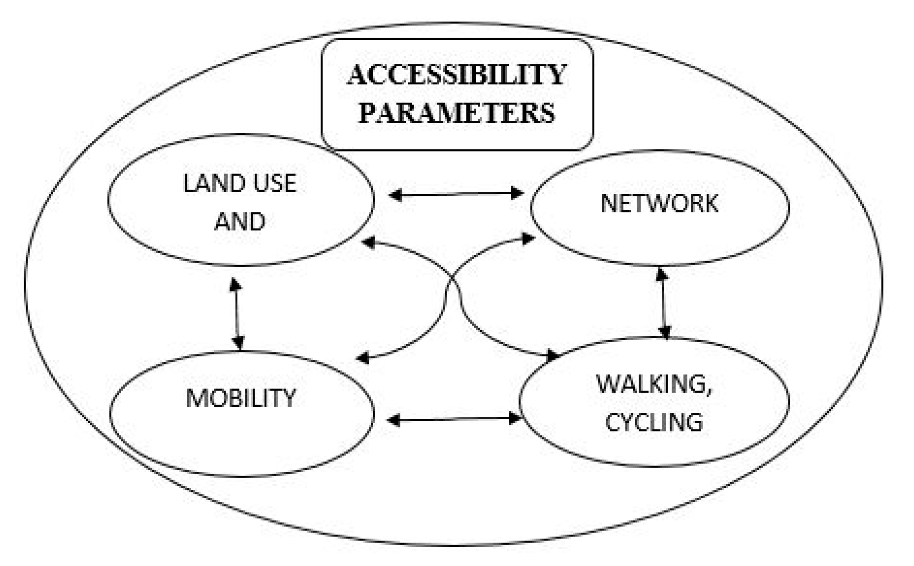
Figure 2.
Framework of the study.
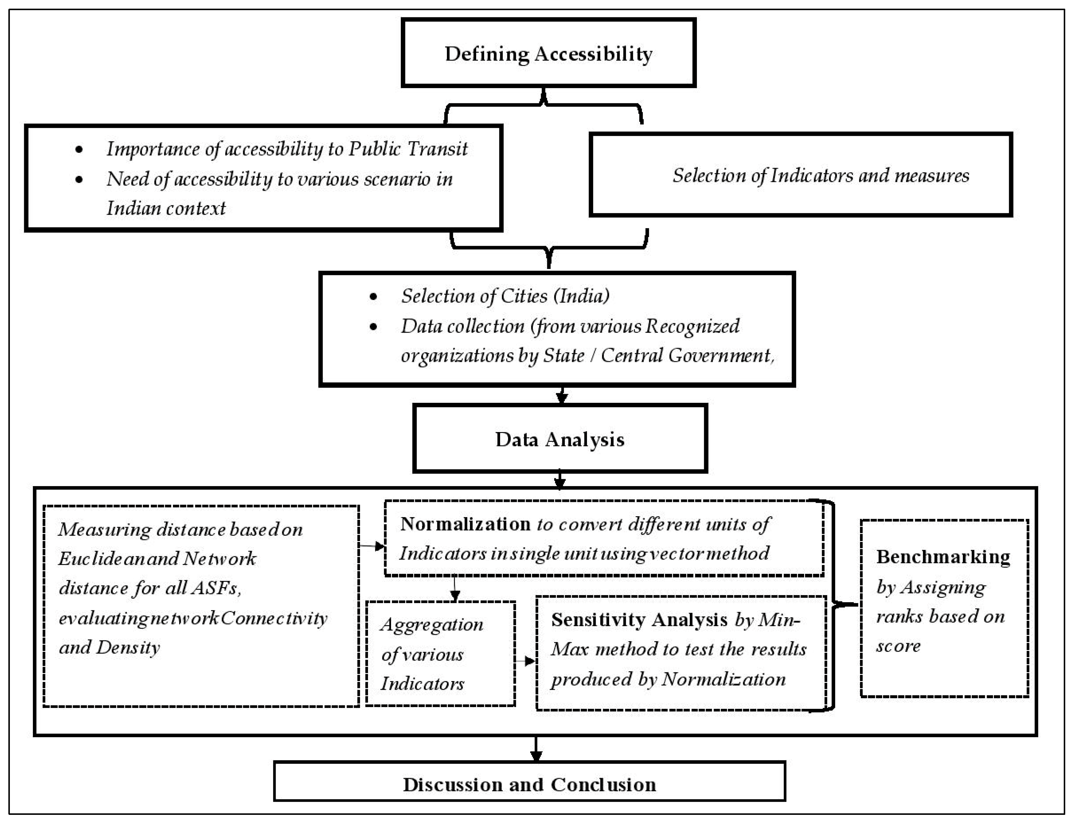
Figure 3.
(a) Average trip length vs. population; (b) Average trip length vs. urban radius. Data source: [77,78].

Figure 4.
Percentage of public transport users in shortlisted cities with population less than 3.0 million according to 2011 census. Data source: [77].
Figure 4.
Percentage of public transport users in shortlisted cities with population less than 3.0 million according to 2011 census. Data source: [77].

Figure 5.
Selected six cities for this study.

Figure 6.
Illustration of methods for data collection.
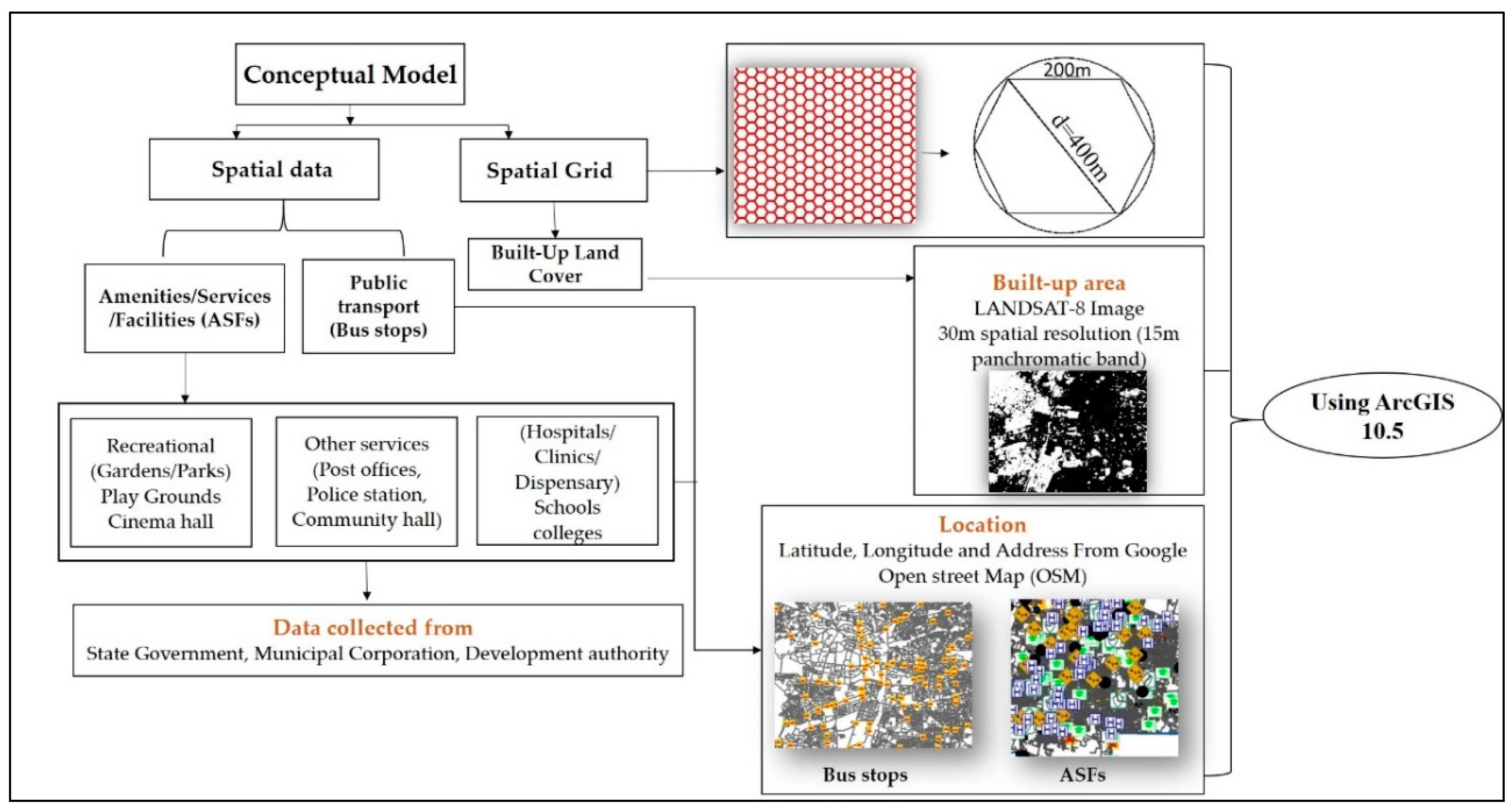
Figure 7.
Overlapping of built-up area with accessibility indices grid.
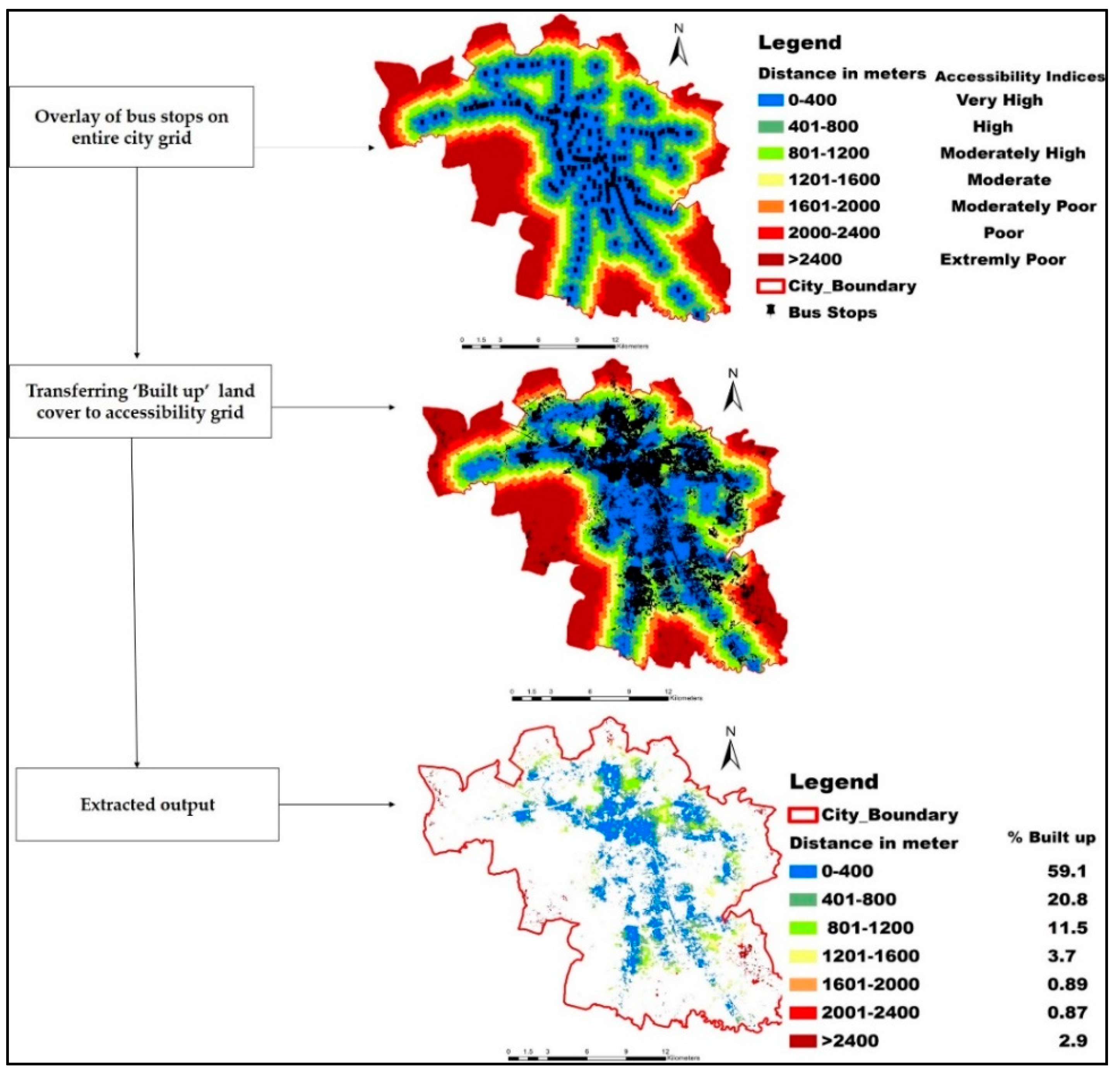
Figure 8.
Built-up area percentage in six cities.
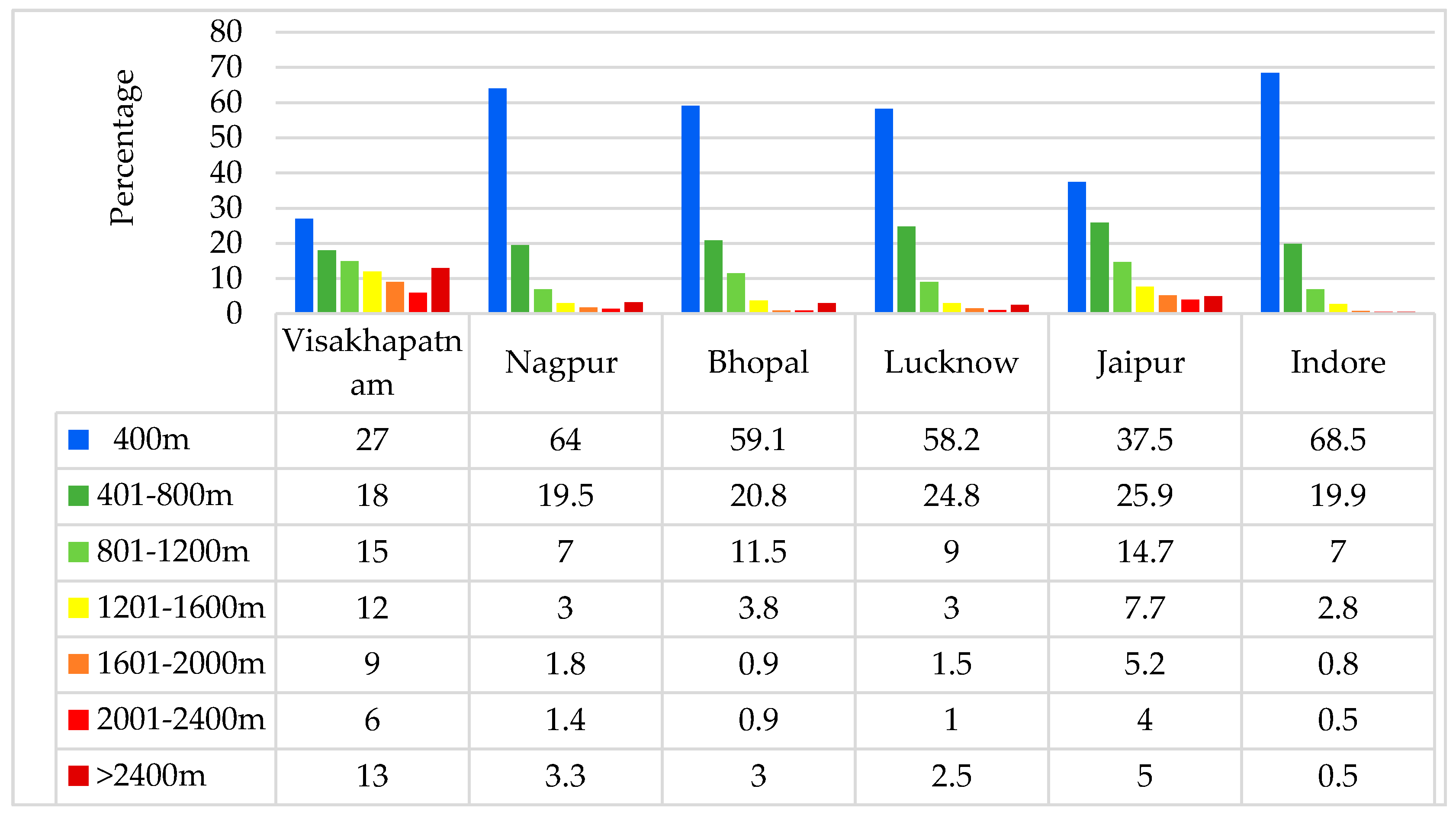
Figure 9.
Spatial evaluation of hospitals and clinics from bus stops using Euclidean distance in six Indian cities.
Figure 9.
Spatial evaluation of hospitals and clinics from bus stops using Euclidean distance in six Indian cities.

Figure 10.
Spatial evaluation of hospitals and clinics from bus stops using network distance in six Indian cities.
Figure 10.
Spatial evaluation of hospitals and clinics from bus stops using network distance in six Indian cities.

Figure 11.
Delineating road network of 0–400 m and 0–1200 m from bus stops in Bhopal city.

Figure 12.
Network density at various levels in all the six cities.

Figure 13.
Detour Index for six cities.
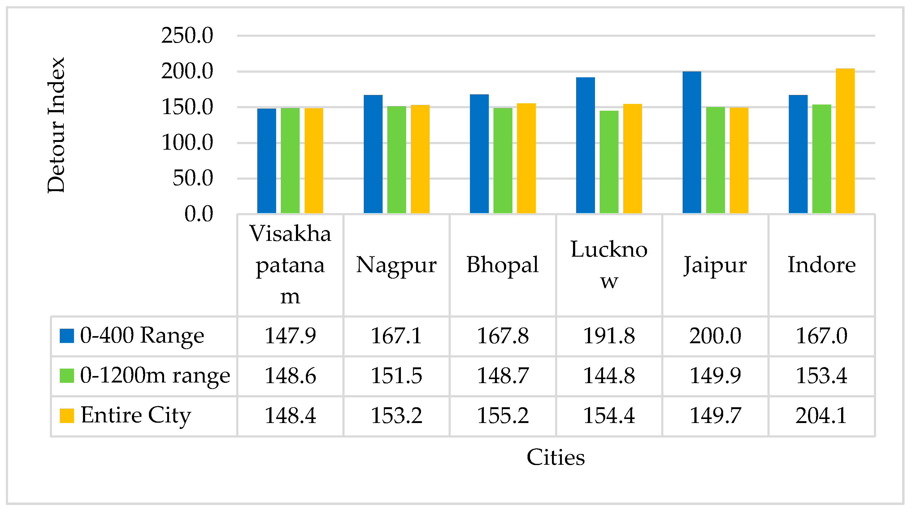
Figure 14.
Comparing ASFs percentage for Euclidean and network distance in 0–400 m range.

Figure 15.
Relating built-up and network density with percentage ASFs.
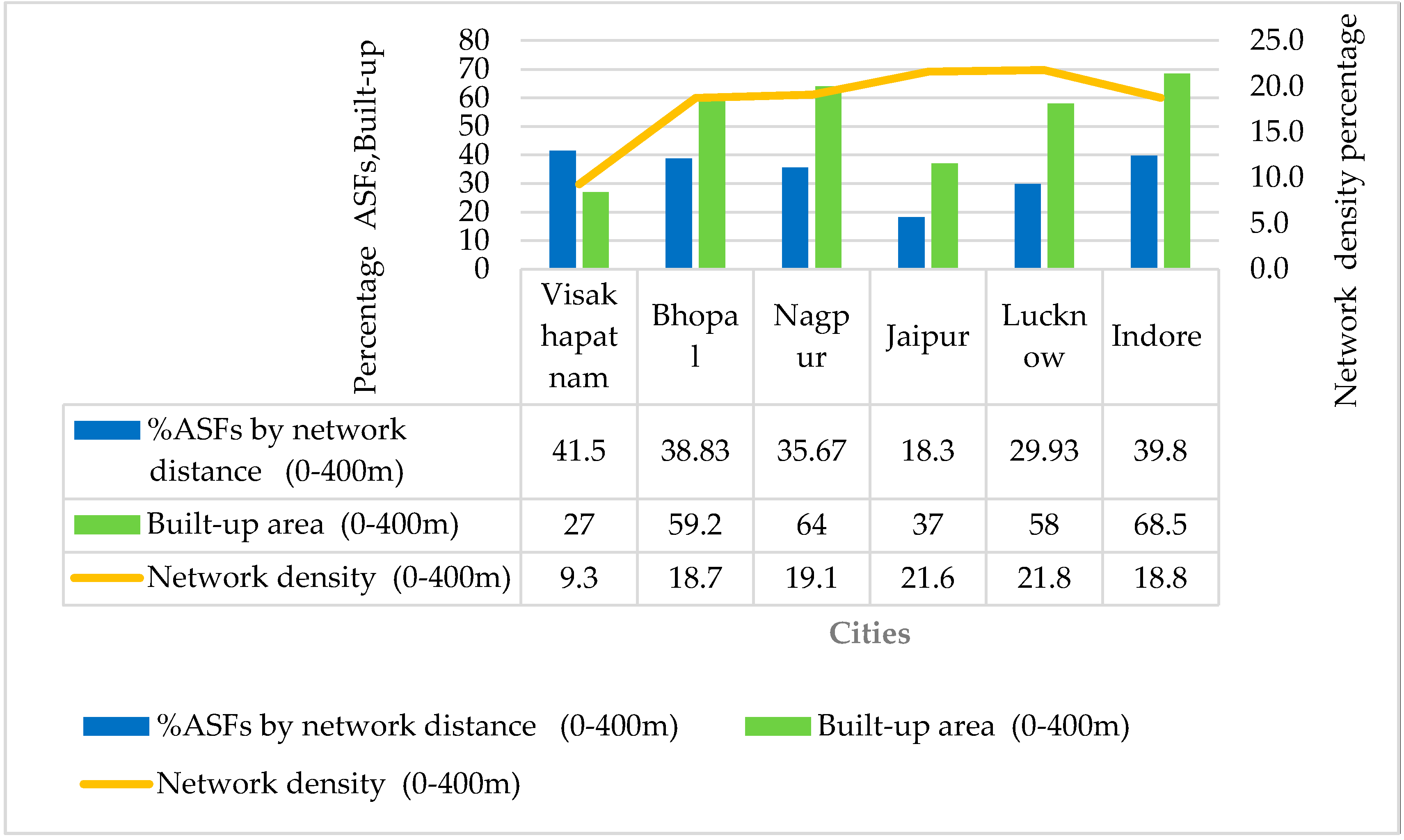
Table 1.
Identified indicators and measures for the study.
| Parameter | Indicator | Measure |
|---|---|---|
| Land cover | Built-up area | The total average percentage of Built-up area in grids |
| The density of ASFs (Amenities, Services, and Facilities) | Number of total opportunities present in the city | |
| Network | Road Network | Length in road network (meters) connecting the closest PT stops to ASFs (shortest path) |
| Network Density | Total road length for each level of accessibility (Square kilometers) | |
| Mobility | Availability of PT | Number of PT stops present in the city |
| Walkability | Proximity | Distance between PT stops from ASFs (Length in meters through road network shortest part, Euclidean distance) |
| Connectivity | Beta Index | Total number of street segments divided by the total number of street nodes |
Table 2.
Identified amenities, services and facilities (ASFs) for the study.
| ASFs | Identified Sectors (Mapping) |
|---|---|
| Amenities | Recreational (Gardens/Parks) Playgrounds Cinema hall |
| Services | Other services (Post offices, Police station, Community hall) |
| Facilities | Hospitals and clinics |
| Schools | |
| colleges |
Table 3.
Summary of studies to identify walking distances.
| City/Country | Distance in Meters For Reaching Amenities/Services | Distance from | Reference |
|---|---|---|---|
| Montreal, Canada | Within 1000 m (preferable) | Resident | [65] |
| New York, Boston, Chicago (U.S.A) | 400, 800, 1600 m | Resident, Transit | [6] |
| Japan | 800, 1600 m | Resident (neighbourhood) | [66] |
| Glasgow, Scotland | 400 m (high-level access) | Resident | [67] |
| Athens, Greece | 500 m < (high-level access) | Resident | [68] |
| Melbourne and Perth Australia | 400 m (high-level bicycle accessibility) | Resident | [69] |
| Catania, south Italy | 300–600 m | Recreational area | [39] |
| Nagpur, India | 400 m (walking Distance) | PT | [70] |
| Ahmedabad, India | 400 m (walking Distance) | PT | [71] |
Table 4.
Colour code used for mapping Euclidean and Network distance.
| Accessibility Indices in Meters | Colour Code for Euclidean/Network Distance | Accessibility Levels |
|---|---|---|
| 0–400 | Very High | |
| 401–800 | High | |
| 801–1200 | Moderate-High | |
| 1201–1600 | Moderate | |
| 1601–2000 | Moderately poor | |
| 2001–2400 | Poor | |
| >2400 | Extremely poor |
Table 5.
Secondary information for six cities.
| Visakhapatnam | Bhopal | Nagpur | Jaipur | Lucknow | Indore | Source | |
|---|---|---|---|---|---|---|---|
| Population In million (2011) | 1.7 | 1.75 | 2.45 | 2.98 | 2.81 | 1.9 | [79] |
| Estimated Population in million (2018) | 1.98 | 1.99 | 2.75 | 3.7 | 3.5 | 2.6 | |
| Density (per Sq. km) | 3364 | 11,057 | 6024 | 11,143 | 8100 | 9718 | |
| Area (Sq. km) | 530.1 | 298.48 | 217.56 | 484.6 | 350 | 135 | [80] |
| The shape of the city | Rayed and Linear | Radial | Ring and Radial | Ring and Radial | Rayed | Ring and Radial | [77] |
| Average Trip length Motor vehicles (Km) | 5.2 | 4.4 | 4.8 | 6.7 | 6 | 4.9 | [78] |
| Distance between bus stops * | 415 * | 395 * | 425 * | 520 * | 391 * | 300 * |
* Authors Calculation.
Table 6.
Extracted Landsat 8 imagery data.
| Scene ID | Path Row | Resolution | Date of Acquisition | |
|---|---|---|---|---|
| Visakhapatnam | LC81410482018112LGN00 | 141/48 | 30 | Oct 2018 |
| Nagpur | LC81440452018325LGN00 | 144/45 | 30 | Nov 2018 |
| Bhopal | LC81450442018332LGN00 | 145/44 | 30 | Nov 2018 |
| Lucknow | LC81440412018261LGN00 | 144/41 | 30 | Oct 2018 |
| Jaipur | LC81470412018362LGN00 | 147/41 | 30 | Oct 2018 |
| Indore | LC81460442019038LGN00 | 146/44 | 30 | Feb 2019 |
Table 7.
Sector-wise Euclidean distance percentage for all six cities within the 0–400 m range.
| ASF’s | Visakhapatnam | Nagpur | Bhopal | Lucknow | Jaipur | Indore |
|---|---|---|---|---|---|---|
| % Accessible (0–400 m) | ||||||
| Recreational Places | 53.1 | 54.5 | 50.0 | 47.2 | 43.8 | 61.5 |
| Playgrounds | 43.3 | 52.6 | 52.9 | 56.9 | 28.8 | 70.6 |
| Cinema Halls | 81.5 | 68.4 | 88.2 | 50.0 | 65.4 | 75.8 |
| Other services (Post offices Police station Community hall) | 53.3 | 63.3 | 68.4 | 53.3 | 46.9 | 74.6 |
| Hospital and clinic | 60.9 | 61.6 | 77.1 | 58.1 | 40.6 | 73.2 |
| Schools | 50.7 | 56.2 | 48.8 | 44.0 | 37.0 | 57.0 |
| colleges | 57.9 | 55.6 | 43.0 | 42.7 | 23.9 | 70.1 |
| average | 57.2 | 58.9 | 61.2 | 50.3 | 40.9 | 69.0 |

Table 8.
Euclidean distance percentage for ASFs combined for the entire range in all six cities.
| % Accessible | % Inaccessible | |||
|---|---|---|---|---|
| Cities | 0–400 m | 401–800 m | 801–1200 m | >1200 m |
| Visakhapatnam | 57.2 | 23.3 | 12.6 | 7.1 |
| Nagpur | 58.9 | 30.9 | 6.8 | 3.4 |
| Bhopal | 61.2 | 25.9 | 9.3 | 3.6 |
| Lucknow | 50.3 | 35.7 | 10.9 | 3.2 |
| Jaipur | 40.9 | 35.8 | 14.6 | 8.7 |
| Indore | 69.0 | 10.0 | 6.6 | 13.5 |
Table 9.
Sector-wise network distance percentage for all six cities within the 0–400 m range.
| ASF’s | Visakhapatnam | Nagpur | Bhopal | Lucknow | Jaipur | Indore |
|---|---|---|---|---|---|---|
| Recreational Places | 38.8 | 31.0 | 28.0 | 29.0 | 25.0 | 27.9 |
| Playgrounds | 23.3 | 26.3 | 48.6 | 22.4 | 12.1 | 33.3 |
| Cinema Halls | 59.3 | 47.4 | 70.6 | 40.0 | 34.6 | 48.5 |
| Other services (Post offices, Police station, Community halls) | 40.1 | 43.9 | 22.8 | 33.3 | 20.4 | 56.4 |
| Hospitals and clinics | 51.1 | 42.1 | 53.8 | 38.4 | 16.3 | 42.4 |
| Schools | 34.5 | 36.5 | 29.6 | 24.6 | 13.0 | 30.7 |
| colleges | 41.1 | 31.8 | 24.3 | 27.1 | 11.0 | 39.4 |
| Average | 41.2 | 37.0 | 39.7 | 30.7 | 18.9 | 39.8 |
Table 10.
Network distance percentage for ASFs combined for the entire range in all six cities.
| % Accessible | % Inaccessible | |||
|---|---|---|---|---|
| Cities | 0–400 m | 401–800 m | 801–1200 m | >1200 m |
| Visakhapatnam | 41.1 | 29.5 | 12.0 | 17.4 |
| Nagpur | 36.9 | 40.1 | 14.0 | 9.0 |
| Bhopal | 39.2 | 32.8 | 13.5 | 14.5 |
| Lucknow | 29.9 | 35.7 | 19.6 | 14.8 |
| Jaipur | 18.9 | 38.2 | 28.4 | 14.5 |
| Indore | 39.8 | 18.5 | 10.3 | 31.5 |
Table 11.
Connectivity index at various levels in all the six cities.
| Cities | Connectivity β = E/V (0–400 m) | Connectivity β = E/V (0–1200 m) | Entire City Network Connectivity β = E/V |
|---|---|---|---|
| Visakhapatnam | 1.49 | 1.45 | 1.43 |
| Nagpur | 1.53 | 1.46 | 1.45 |
| Bhopal | 1.57 | 1.52 | 1.46 |
| Lucknow | 1.57 | 1.4 | 1.39 |
| Jaipur | 1.53 | 1.4 | 1.39 |
| Indore | 1.41 | 1.39 | 1.36 |
Table 12.
Mean Difference between Euclidean and network distance for overall ASFs in selected six cities.
Table 12.
Mean Difference between Euclidean and network distance for overall ASFs in selected six cities.
| (n) | Mean (M) | Standard Deviation (S.D) | Range | |||||
|---|---|---|---|---|---|---|---|---|
| Cities | Euclidean | Network | Difference | Euclidean | Network | Euclidean | Network | |
| Visakhapatnam | 525 | 566.7 | 841.1 | 274.4 | 611.4 | 998.4 | 3170.9 | 5367.1 |
| Nagpur | 1023 | 427.6 | 640 | 212.4 | 386 | 540.3 | 2376.4 | 3548.3 |
| Bhopal | 748 | 501.2 | 777.8 | 276.6 | 591.1 | 871.6 | 3890.9 | 5468.3 |
| Lucknow | 996 | 472.7 | 730.1 | 257.4 | 371 | 525.8 | 2394.8 | 3298.4 |
| Jaipur | 1103 | 596.8 | 914.2 | 317.4 | 435.8 | 616 | 2224.3 | 3380 |
| Indore | 808 | 337.3 | 566.2 | 228.9 | 262.2 | 384.5 | 1391 | 1922.6 |
Table 13.
The normalized score for very high accessibility range 0–400 m Euclidean distance.
| Cities | %ASFSs | %Built-Up | Mean Distance | Average Score | Rank |
|---|---|---|---|---|---|
| Visakhapatnam | 0.409 | 0.203 | 0.536 | 0.383 | 6 |
| Nagpur | 0.423 | 0.480 | 0.559 | 0.487 | 3 |
| Bhopal | 0.440 | 0.444 | 0.625 | 0.503 | 2 |
| Lucknow | 0.359 | 0.435 | 0.615 | 0.470 | 4 |
| Jaipur | 0.294 | 0.278 | 0.578 | 0.390 | 5 |
| Indore | 0.495 | 0.514 | 0.650 | 0.553 | 1 |
Table 14.
The normalized score for moderate-high accessibility range 0–1200 m Euclidean distance.
| Cities | %ASFSs | %Built-Up | Mean Distance | Average Score | Rank |
|---|---|---|---|---|---|
| Visakhapatnam | 0.415 | 0.286 | 0.610 | 0.437 | 5 |
| Nagpur | 0.428 | 0.429 | 0.634 | 0.497 | 2 |
| Bhopal | 0.432 | 0.435 | 0.535 | 0.467 | 4 |
| Lucknow | 0.433 | 0.433 | 0.596 | 0.488 | 3 |
| Jaipur | 0.349 | 0.371 | 0.508 | 0.409 | 6 |
| Indore | 0.387 | 0.469 | 0.695 | 0.517 | 1 |
Table 15.
The normalized score for very high accessibility range 0–400 m network distance.
| Cities | %ASFSs | Connectivity | Mean Distance | Average Score | Rank |
|---|---|---|---|---|---|
| Visakhapatnam | 0.478 | 0.401 | 0.615 | 0.498 | 2 |
| Nagpur | 0.429 | 0.412 | 0.587 | 0.476 | 4 |
| Bhopal | 0.452 | 0.422 | 0.647 | 0.507 | 1 |
| Lucknow | 0.348 | 0.422 | 0.586 | 0.452 | 5 |
| Jaipur | 0.220 | 0.412 | 0.527 | 0.386 | 6 |
| Indore | 0.462 | 0.379 | 0.599 | 0.480 | 3 |
Table 16.
The normalized score for moderate-high accessibility range 0–1200 m network distance.
| Cities | %ASFs | Connectivity | Mean Distance | Average Score | Rank |
|---|---|---|---|---|---|
| Visakhapatnam | 0.401 | 0.412 | 0.581 | 0.465 | 3 |
| Nagpur | 0.443 | 0.415 | 0.608 | 0.488 | 2 |
| Bhopal | 0.416 | 0.432 | 0.642 | 0.496 | 1 |
| Lucknow | 0.414 | 0.398 | 0.557 | 0.456 | 5 |
| Jaipur | 0.416 | 0.398 | 0.550 | 0.454 | 6 |
| Indore | 0.354 | 0.395 | 0.622 | 0.457 | 4 |
Table 17.
Comparison of normalization results between min.
| Min-Max Method | Vector Method | |||||
|---|---|---|---|---|---|---|
| City | Score | Rank | Difference | Score | Rank | Difference |
| Indore | 1.00 | 1 | 0.55 | 1 | ||
| Bhopal | 0.76 | 2 | 0.24 | 0.50 | 2 | 0.05 |
| Nagpur | 0.59 | 3 | 0.18 | 0.49 | 3 | 0.01 |
| Lucknow | 0.58 | 4 | 0.01 | 0.47 | 4 | 0.02 |
| Jaipur | 0.31 | 5 | 0.27 | 0.39 | 5 | 0.09 |
| Visakhapatnam | 0.19 | 6 | 0.12 | 0.38 | 6 | 0.01 |
© 2020 by the authors. Licensee MDPI, Basel, Switzerland. This article is an open access article distributed under the terms and conditions of the Creative Commons Attribution (CC BY) license (http://creativecommons.org/licenses/by/4.0/).
Share and Cite
MDPI and ACS Style
Yenisetty, P.T.; Bahadure, P. Measuring Accessibility to Various ASFs from Public Transit using Spatial Distance Measures in Indian Cities. ISPRS Int. J. Geo-Inf. 2020, 9, 446. https://doi.org/10.3390/ijgi9070446
AMA Style
Yenisetty PT, Bahadure P. Measuring Accessibility to Various ASFs from Public Transit using Spatial Distance Measures in Indian Cities. ISPRS International Journal of Geo-Information. 2020; 9(7):446. https://doi.org/10.3390/ijgi9070446
Chicago/Turabian StyleYenisetty, Pavan Teja, and Pankaj Bahadure. 2020. "Measuring Accessibility to Various ASFs from Public Transit using Spatial Distance Measures in Indian Cities" ISPRS International Journal of Geo-Information 9, no. 7: 446. https://doi.org/10.3390/ijgi9070446
Note that from the first issue of 2016, this journal uses article numbers instead of page numbers. See further details here.