Article

Flash Flood Susceptibility Assessment Based on Geodetector, Certainty Factor, and Logistic Regression Analyses in Fujian Province, China

1
School of Civil Engineering and Geomatics, Southwest Petroleum University, Chengdu 610500, China
2
State Key Laboratory of Resources and Environmental Information System, Institute of Geographic Sciences and Natural Resources Research, CAS, Beijing 100101, China
3
University of Chinese Academy of Sciences, Beijing 100049, China
4
School of Geoscience and Technology, Southwest Petroleum University, Chengdu 610500, China
*
Author to whom correspondence should be addressed.
ISPRS Int. J. Geo-Inf. 2020, 9(12), 748; https://doi.org/10.3390/ijgi9120748
Submission received: 10 November 2020 / Revised: 5 December 2020 / Accepted: 10 December 2020 / Published: 14 December 2020

Abstract

:
Flash floods are one of the most frequent natural disasters in Fujian Province, China, and they seriously threaten the safety of infrastructure, natural ecosystems, and human life. Thus, recognition of possible flash flood locations and exploitation of more precise flash flood susceptibility maps are crucial to appropriate flash flood management in Fujian. Based on this objective, in this study, we developed a new method of flash flood susceptibility assessment. First, we utilized double standards, including the Pearson correlation coefficient (PCC) and Geodetector to screen the assessment indicator. Second, in order to consider the weight of each classification of indicator and the weights of the indicators simultaneously, we used the ensemble model of the certainty factor (CF) and logistic regression (LR) to establish a frame for the flash flood susceptibility assessment. Ultimately, we used this ensemble model (CF-LR), the standalone CF model, and the standalone LR model to prepare flash flood susceptibility maps for Fujian Province and compared their prediction performance. The results revealed the following. (1) Land use, topographic relief, and 24 h precipitation (H24_100) within a 100-year return period were the three main factors causing flash floods in Fujian Province. (2) The area under the curve (AUC) results showed that the CF-LR model had the best precision in terms of both the success rate (0.860) and the prediction rate (0.882). (3) The assessment results of all three models showed that between 22.27% and 29.35% of the study area have high and very high susceptibility levels, and these areas are mainly located in the east, south, and southeast coastal areas, and the north and west low mountain areas. The results of this study provide a scientific basis and support for flash flood prevention in Fujian Province. The proposed susceptibility assessment framework may also be helpful for other natural disaster susceptibility analyses.

1. Introduction

Flash floods are a type of natural disaster that often occurs in mountainous areas and results in tremendous damage to infrastructure, human lives, and property [1]. Mountain areas in China represent more than two-thirds of the total area, and thus, the country is prone to flash floods [2]. A statistic from the National Mountain Flood Disaster Investigation Project shows that China experienced more than 10,000 flash floods between 2010 and 2016, which led to the disappearance or death of at least 4800 people [3]. Fujian is considered to be the province that has experienced the most severe flash flood disasters in China; about 95% of the entire regions and 84% of the population are directly threatened by flash floods [4]. Examples of some recent flash floods in Fujian include Yongtai County in 2003, Liancheng County in 2010, and Changle City in 2015. The flash flood in Yongtai County caused more than 14 million USD worth of damage to roads, buildings, and agricultural land, while the flash flood in Liancheng city affected about 42.3 thousand people and led to the rapid relocation of 14.2 thousand people. Therefore, the recognition and evaluation of regions susceptible to flash floods in Fujian Province are necessary and urgently needed to prevent and alleviate the damage and loss caused by flash floods.
Flash flood susceptibility assessment is a significant tool in flash flood disaster prevention [5]. The most common models of flash flood susceptibility assessment can be broadly classified into three categories: hydrological methods, statistical methods, and machine learning algorithms. In terms of hydrological methods, HYDROTEL [6], SWAT [7], and WetSpa [8] are the three most commonly used models. Although they have many advantages, these models are insufficient in that they require more information about the mechanism and process of flooding and are only applicable to a single flood surface or a small study area. In contrast to the hydrological methods, the statistical methods, such as the frequency ratio (FR) method [9], the multiple criteria decision methods [10], and the weights-of-evidence (WOE) method [11], and the machine learning methods, such as the support vector machine (SVM) [12], the artificial neural network (ANN) [13], the random forest (RF) method [14], and other models, are more frequently used for the quantitative assessment of flash flood susceptibility over large-scale areas (province and country scale).
Although these methods have been successfully applied in many flash flood studies, at present, there are still two common problems in flash flood susceptibility assessments. On the one hand, there is no consensus among hydrologists as to which model has the highest accuracy, due to the complex mechanisms linking flash floods and their conditioning factors [15]. Specifically, almost all of the statistical methods and machine learning methods have their own defects. For example, machine learning methods like the ANN are regarded as a black box and require a large amount of high-precision basic data and enough computational power during designing, building, and verification processes [16]. For statistical methods, strict assumptions need to be made before the research is conducted, which is considered to be the disadvantage of such methods, and it is difficult to use them in practical applications. Moreover, some qualitative approaches, such as the analytic hierarchy process (AHP), need expert judgments and contain many prejudices. On the other hand, we lack a valid method for choosing assessment indicators before establishing a model [17]. Superfluous assessment indicators augment the instability of the model and reduce the accuracy of the prediction [18]. Due to this problem, many researchers have used factor analysis [19], principal component analysis [20], and the optimization technique [21] to screen the factors that have significant influences on floods. There is no doubt that these methods ultimately enhance the reliability of flood susceptibility assessments to some extent. However, it is worth noting that these methods do not consider the spatial pattern characteristics of each conditioning factor or historical flood events, which also decreases their accuracy.
To solve the first problem, multivariate statistical analysis (MSA) models such as logistic regression (LR), which is easy to run and has a similar or better predictive power, can be used as an appropriate replacement [15]. Although multivariate LR is a steady approach compared with other methods, it has some restrictions when executing the bivariate statistical analysis (BSA) because it employs the classifications as an indicator and does not consider them in the regression process [22]. In contrast to LR, the certainty factor (CF) evaluates the impact of the classifications of each assessment indicator on the flash flood, but it overlooks the relationship between the assessment indicators. Tien Bui [15] pointed out that the different classifications of the conditioning factors have a greater influence than the different conditioning factors themselves in natural disaster assessment and mapping. Therefore, to consider the weight of each factor classification and the weights of the factors themselves at the same time, we combined the CF and LR models and applied them into the flash flood susceptibility assessment field for the first time. The highlight of this method is that it uses the CF to perform the BSA in order to acquire the information value of the classifications of each independent variable, and it uses these values as the input data for the LR. This integrated approach not only overcomes the disadvantages of using either the CF or LR alone, but it also avoids the complicated and incomprehensible calculation processes of the ANN and other machine learning methods. To solve the second problem, we used Geodetector to screen the conditioning factors that have a high spatial correlation with the distribution of historical flash floods. Geodetector is a classical spatial statistical method that can be used to evaluate the relative importance of each factor, which promote or cause a geographical phenomenon [23]. In recent years, Geodetector has been widely used in social science [24], natural science [25], human health [26], and other fields to explain the spatial distribution patterns of spatial data.
The main objective of this research is to assess the flash flood susceptibility of Fujian Province using CF, LR, and their ensemble model (CF-LR), and to compare their prediction performances. The specific processes consist of the following aspects: (i) use double standards, including the Pearson correlation coefficient (PCC) and Geodetector, to screen the assessment indicators; (ii) use CF, LR, and CF-LR models to prepare flash flood susceptibility maps; and (iii) use statistical evaluation measures and the receiver operating characteristic (ROC) curve to assess the efficiencies and precisions of the three models.

2. Materials and Methods
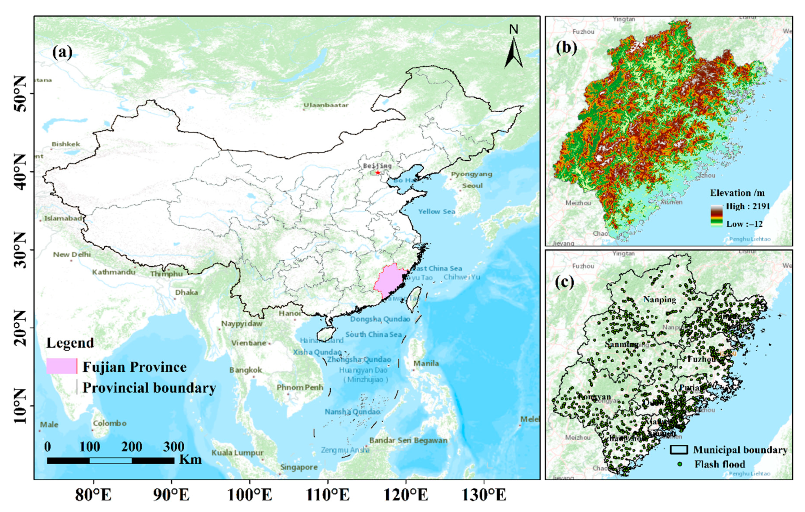
2.1. Study Area

Fujian Province is located in southeastern China (115°40′–120°30′ E and 23°30′–28°20′ N) and covers an area of roughly 120,000 km2 (Figure 1a). Fujian has a population of 39.11 million and a regional gross domestic product of 3.22 trillion RMB at the end of 2017 (http://tjj.fujian.gov.cn/tongjinianjian/dz2018/index-cn.htm) [27]. In terms of climate and hydrology, Fujian Province has a subtropical monsoon climate with abundant rainfall and rich heat. The long-term annual average temperature of Fujian Province ranges from 17 to 21 °C, which increases from northwest to southeast. The annual average rainfall varies from the coastal area and islands to the northwestern mountain areas, increasing from 1200 to 2200 mm, respectively [28]. There are many rivers in Fujian Province, and the density of the river network is 0.1 km/km2. In terms of the landforms and geomorphological characteristics, the study area mainly consists of four types: river valley, basin, mountain, and hill. Among them, the mountains and hills account for more than 80% of the total area. The minimum and maximum elevations are 12 meters below the average sea level and 2191 meters above the average sea level (Figure 1b), respectively. For the geological environment, the strata of Fujian Province are mainly composed of sedimentary rocks, metamorphic rocks, and volcanic rocks, accounting for 59.09% of the total land area [29]. The lithology is mainly granite, but also syenite, gabbro, diabase, amphibolite, mixed granite, and others are present. Furthermore, Fujian Province is situated on the southeast margin of Eurasia plate and adjacent to the Pacific plate. The geological structure is complex, magmatic activity is frequent, and the entire region is located in the second uplift belt of the Neocathaysian giant structural system, and the eastern end of the Nanling latitudinal structural system [30]. These two structural systems constitute the most powerful and active structure in Fujian Province.

2.2. Materials

2.2.1. Flash Flood Inventory Map

Identifying future flash flood susceptible zones requires a complete understanding of historical flash flood events in the study area [31] because the accuracy of historical flash flood information often has a significant impact on the precision of the assessment results [32]. The flash flood inventory maps used in this study were obtained from the National Flash Flood Investigation and Evaluation Project (NFFIEP), which was launched in 2013 by the Ministry of Water Resources of China and the Ministry of Finance of China [33]. This project investigated and recorded on a national scale the flash flood events that occurred from 1949 to 2015. The longitude, latitude, time, casualties, and economic losses of these historical flash flood events all passed strict quality inspection by the experts and scholars of the China Institute of Water Resources and Hydropower [34]. Thus, the accuracy of these data is very reliable and has been verified in several published articles [2,3].
The total number of historical flash flood events in Fujian Province is 1566 (Figure 1c). These historical flash flood points were assigned a value of 1 and were randomly divided into two categories containing 80% and 20% of the events [35], which were used as positive training samples and positive test samples, respectively. Flash flood susceptibility assessment can be thought of as a binary classification; the flash flood exponent is classified into two types: flooding and nonflooding, or existence and nonexistence [36]. Therefore, the inclusion of non-flash flood events would probably improve the precision of assessment results. Based on this assumption, an equal number of non-flash flood points (assigned a value of 0) were chosen as negative training samples and negative test samples using the random selection tool in ArcGIS (version 10.2). Therefore, a total of 2506 training samples and 626 validation samples were obtained.

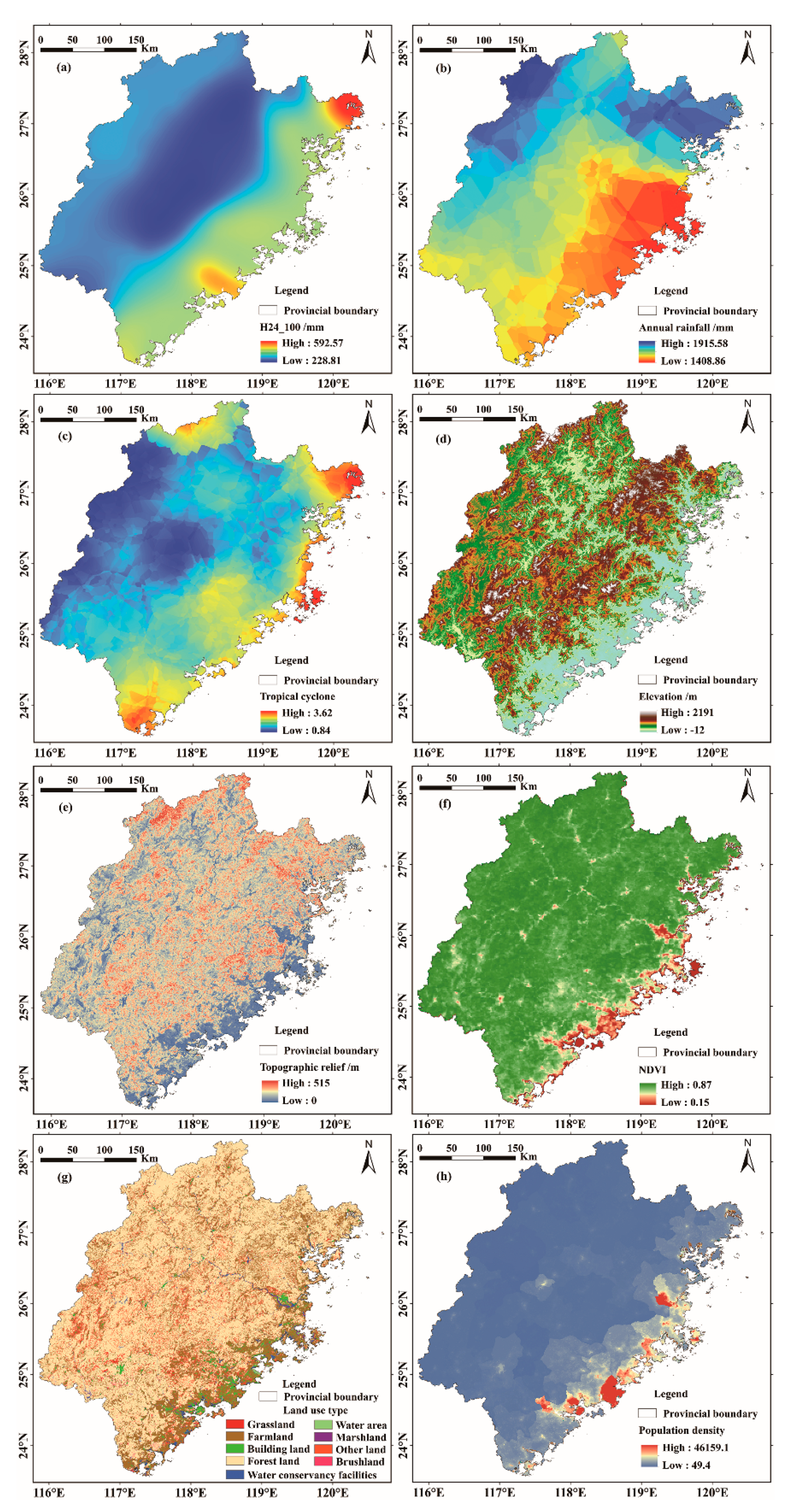
2.2.2. Flash Flood Conditioning Factors

A large number of studies have shown that the formation and occurrence of flash floods are mainly related to three major factors: precipitation, topography and geology, and human activities [37,38,39]. Based on the selection principles (e.g., objectivity, representativeness, and availability) of the conditioning factors and the formation mechanism of the flash floods, a total of 14 conditioning factors were preliminarily selected: (1) elevation, (2) slope, (3) topographic relief, (4) normalized difference vegetation index (NDVI), (5) land use type, (6) soil type, (7) soil depth, (8) distance from rivers, (9) 6 h precipitation (H6_100) within a 100-year return period, (10) 24 h precipitation (H24_100) within a 100-year return period, (11) annual rainfall, (12) tropical cyclone index, (13) population density, and (14) economic density. A concise description of each conditioning factor used in this study is provided in Table 1. Particularly, it should be mentioned that the interpolation analysis, raster conversion, resample, and other tools in ArcGIS 10.2 were applied to process the raw datasets. Ultimately, all of the 14 different types of conditioning factor data were transformed into raster data with a spatial resolution of 30 m × 30 m.
(1)
Elevation
Elevation is one of the most crucial factors that influence flooding [40]. The flow of the flood mainly relies on its own gravity, i.e., transferring from higher to lower elevations, which indicates that lower elevation areas are more prone to flooding. The original elevation data came from the advanced spaceborne thermal emission and reflection radiometer global digital elevation model (ASTER GDEM), which was supplied by the Geospatial Data Cloud (www.gscloud.cn).
(2)
Slope
Slope is a significant physiographic characteristic, and it plays an important role in flash flood susceptibility assessment [41] because it not only controls the flow speeds of floods, but also affects surface runoff and infiltration. Flat areas with lower elevations may have shorter periods of time to form real-time flash floods than steeper areas with higher elevations. The slope map was calculated after the depression areas of the DEM were filled.
(3)
Topographic Relief
Topographic relief is another important topographic factor. It refers to the difference between the altitude of the highest and lowest point in a specific area, which can directly reflect the form of the surface. After DEM depressions were filled, the best statistical unit was calculated by the mean change point analysis method [42], with an 11 × 11 grid size (area of 330 m × 330 m). We calculated the topographic relief from the DEM by using the focal statistics tool in ArcGIS (version 10.2).
(4)
NDVI
Vegetation coverage is deemed to be one of the most significant factors restraining flash floods. Because vegetation can absorb water through roots and leaves, it effectively reduces the erosion of the slope by surface runoff. We used the normalized difference vegetation index (NDVI) to reflect the vegetation coverage in the study area. These data are freely available from the National Earth System Science Data Center (http://www.geodata.cn/).
(5)
Land Use Type
Land use types can directly and indirectly affect the components of hydrological processes (e.g., evapotranspiration, runoff generation, and infiltration) and sediment transport [43]. The land use type data were obtained from the NFFIEP database.
(6)
Soil Type
Different soil types have different structures. When soil interacts with vegetation, the permeability and erosion resistance of the soil will change [16]. The soil type data were also obtained from the NFFIEP database.
(7)
Soil Depth
The soil depth mainly includes the effective soil layer depth and the soil depth, which can more intuitively express the properties of the soil [44]. Generally speaking, the higher the value of soil depth, the more conducive to the infiltration and accumulation of water, which reduces surface runoff. The soil depth map was obtained from the China Dataset of Soil Properties for Land Surface Modeling [45].
(8)
Distance from Rivers
Areas near rivers are seriously influenced by flash floods, and the influence of this factor decreases gradually with increasing distance from the riverbed [46]. The distance from the rivers data layer was calculated by imposing multifarious buffer zones every 2000 m around the four-level river systems.
(9)
Rainstorm Factors
Heavy rainfall over a short period of time is one of the main causes of flash floods. Therefore, based on previous research results [47], we selected the 6 h precipitation (H6_100) and 24 h precipitation (H24_100) within a 100-year return period as rainstorm factors of different intensities. The rainstorm factor data were obtained from the NFFIEP database, and were converted to raster data with a resolution of 30 m × 30 m using the kriging interpolation method in ArcGIS10.2.
(10)
Annual Rainfall
According to Arpita Nandi [31], thirty-year mean annual rainfall was selected as one of the assessment indicators. Similarly, we chose the data of the Annual Data Set of China’s Ground Annual Value (1981–2010) and used the kriging method in the ArcGIS 10.2 software to interpolate the data measured at precipitation stations in the study area to obtain the annual rainfall raster data. The data from each precipitation station are freely available from the National Meteorological Information Center (http://data.cma.cn/).
(11)
Tropical Cyclone Index
A tropical cyclone is a cyclonic eddy that occurs over tropical and subtropical oceans. Tropical cyclone tracks record a sequence of points every 6 h, and the values of these points can be downloaded from the Tropical Cyclone Data Center, China Meteorological Administration (http://www.typhoon.org.cn). The values of these points were also converted into raster data through interpolation.
(12)
Population Density
The population density is the number of people per 1 km2 [48]. Previous studies have shown that human activities have a hysteresis effect on flash floods. Therefore, the population density data from 2010 were selected as one of the human activity factors. The population density data can be downloaded for free from the Resource and Environment Data Cloud Platform (http://www.resdc.cn/).
(13)
Economic Density
Economic density refers to the ratio of the gross domestic product (GDP) to the analytical units, and it indicates the level of socioeconomic development in the area. The economic density can indirectly reflect the intensity of human activities. Therefore, we used the economic density data for 2010 as the second human activity indicator.

2.3. Methods

2.3.1. Pearson Correlation Coefficient

The Pearson correlation coefficient (PCC) is a popular statistical tool for testing the linear correlation between variables x and y. The PPC varies between −1 and +1, and it can be calculated using the following equation:
R = i = 1 n x i y i i = 1 n x i i = 1 n y i n ( i = 1 n x i 2 ( i = 1 n x i ) 2 n ) ( i = 1 n y i 2 ( i = 1 n y i ) 2 n )
where R is the PCC between variables x and y, and n is the number of variables x and y. The PCC value and the specific corresponding correlation levels are presented in Table 2 [33].

2.3.2. Geodetector

Geodetector is a classic statistical method used to explore the spatially stratified heterogeneity and to reveal the correlation between the independent variable x and the dependent variable y [17]. Therefore, it can be used to select conditioning factors. The Geodetector makes few hypotheses about the input data, so it has been widely used in geoscience and remote sensing [17,49,50].
The most important assumption of Geodetector is that if an independent variable x (e.g., the annual rainfall) has a significant effect on a dependent variable y (e.g., the flash floods density), the spatial distribution characteristics of both x and y should be similar. This similarity can be determined by the rate of the local variance to the global variance [51], and the specific principle is as follows:
q = 1 1 N σ 2 h = 1 n N h σ h 2
where n is the number of strata in the layer x; Nh is the number of samples in the hth stratum; N is the total number of samples in the study area; σ h 2 is the variance of variable y in the hth stratum; and σ 2 is the variance of variable y in the entire study area. The value of q is between 0 and 1, and large values of q reflect a large contribution of the layer x to flash flood occurrence.

2.3.3. Certainty Factor

The CF model is one of the most effective strategies for solving the problem of combining different data layers and the heterogeneity and uncertainty of the input data [52]. It is a probability function that was originally proposed by Shortliffe and Buchanan in 1975 and was later improved by Heckerman (1986) [53]. It can be expressed as follows:
C F = { p p a p p s p p a ( 1 p p s ) , p p a p p s p p a p p s p p s ( 1 p p a ) , p p a < p p s
where CF is the certainty factor and PPa is the conditional probability of the flash flood event occurring in category a of the conditioning factor map (e.g., grassland in the land use layer). PPs is the prior probability of the total number of flash flood events in the study area and the value of PPs remains the same when the study area is determined.
The range of the variation in the certainty factor is [−1, +1]. The minimum value of −1 corresponds to completely false and the maximum value of +1 corresponds to completely true. A positive value signifies an increasing certainty of flash flood occurrence, while a negative value signifies a decreasing certainty. When the value is close to 0, the conditional probability is very close to the prior probability. Thus, it is difficult to give any information about the certainty of the occurrence of a flash flood [54].
After obtaining the CF values of the different flash flood conditioning factors, the values were combined pairwise using the CF combination rule. For example, X and Y are two different layers and they can be combined as follows:
Z = { X + Y X Y X , Y 0 X + Y 1 m i n ( | X | , | Y | ) X * Y < 0 X + Y + X Y Y < 0
Using the computation rule in Equation (4), the pairwise combination was calculated repeatedly until all of the CF layers were overlaid to obtain the flash flood susceptibility map.

2.3.4. Logistic Regression

Logistic regression (LR) is one of the most popular methods used in natural hazard susceptibility assessments [55,56,57]. This method has two obvious advantages: ① the data used do not need a normal distribution and ② the data types of the conditioning factors are unrestricted (i.e., they can be discrete, continuous, or any combination of the two types).
LR consists of an independent variable X and dependent variable Y. Among them, the independent variable X can have two or more values, while the dependent variable Y can only have two values. When LR is applied to flash flood susceptibility analysis, flash flood inventories are used as the dependent variable representing the existence (value of 1) or nonexistence (value of 0) of a flash flood. LR can be used to determine the logistic coefficients of all of the assessment indicators, which can be used with the geographic information system (GIS) to predict the future flash flood or non-flash flood status of a study area [32]. Thus, the relationship between the flash flood probability index (P) or the non-flash flood probability index (Q) and the factors can be expressed as follows:
P = 1 1 + e Z = e Z 1 + e Z
Q = 1 P = 1 1 + e Z
Z = B 0 + B 1 X 1 + B 2 X 2 + + B n X n
where B0 is a constant value that represents the intercept of the LR model; B1, B2, , Bn represent the logistic coefficients (i.e., the weights of the conditioning factors); X1, X2, , Xn represent the assessment indicators (e.g., slope, annual rainfall, and elevation); and Z is an intermediate variable.

3. Results

3.1. Screening of the Assessment Indicators

3.1.1. Correlation Matrix of the Conditioning Factors

The correlation matrix between the conditioning factors was generated using SPSS 25, and the results are shown in Table 3. The correlations between most of the conditioning factors are very poor, indicating that these conditioning factors are independent of each other. Nonetheless, a very strong correlation exists between economic density and population density (R = 0.81) and between H6_100 and H24_100 (R = 0.92).

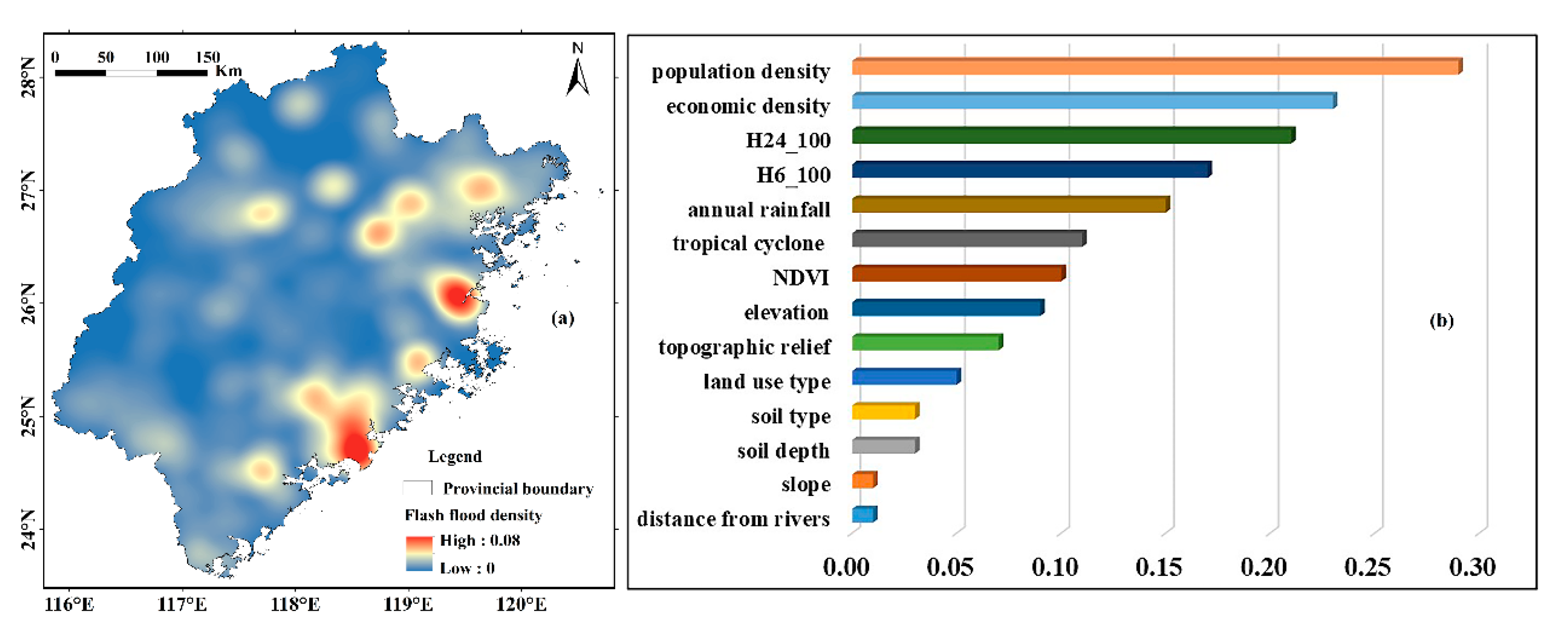
3.1.2. Implementation of Geodetector

To calculate the rate of the local variance to the global variance, we implemented the following steps: (1) 2000 random points were selected in the study area using the random selection tool in ArcGIS, and the specific working principle of random selection tool can be found at https://desktop.arcgis.com/en/arcmap/latest/tools/data-management-toolbox/how-create-random-points-works.htm. (2) The values of each conditioning factor were extracted to all random points and then divided into five categories by using the natural break method. (3) The density of the historical flash flood points (Figure 2a) was calculated and taken as the variable Y. (4) The value of variable Y was extracted at all of the random points. (5) The attribute values of all points were exported as the input table to Geodetector, and the output result of each conditioning factor calculated by Geodetector is presented in Figure 2b. The first 10 variables with q values of greater than 0.05 were selected. These factors were population density (q = 0.29), economic density (q = 0.23), H24_100 (q = 0.21), H6_100 (q = 0.17), annual rainfall (q = 0.15), tropical cyclone (q = 0.11), NDVI (q = 0.1), elevation (q = 0.09), topographic relief (q = 0.07), and land use (q = 0.05).
Finally, based on the analysis results of the PCC and Geodetector, H24_100, annual rainfall, tropical cyclone index, elevation, topographic relief, NDVI, land use type and population density were selected as the final assessment indicators (Figure 3).

3.2. Susceptibility Assessment and Mapping

3.2.1. Implementation of the Certainty Factor

Using Equation (3), the CF values were calculated for the classification levels of each assessment indicator by overlaying and reckoning the flash flood frequency. The CF values of the different classification levels of the eight assessment indicators are presented in Table 4.
The H24_100 classification of 450–550 mm has the maximum CF value (0.74), followed by the 350–450 mm classification (0.37). The minimum CF value (–0.42) is for the H24_100 classification of <250 mm. This indicates that the incidence of flash flood increases with increasing H24_100 to a certain extent. However, in the end, it decreases.
In terms of land use, the CF values of farmland, building land, water conservancy facilities, marshland, and other land are positive, with the highest value (0.93) for building land. In contrast, based on their negative CF values, grassland, forest land, brushland, and water area are less prone to flash floods.
In terms of topographic relief, the CF value is positive (0.76) only for the <50 m classification. As the topographic relief increases, the CF value becomes closer to −1, and the >300 m classification does not induce flash flood in this area.
The CF values of the tropical cyclone index are negative for the ranges of <1.4, 1.4–2, >3.2, with the minimum value (−0.88) occurring for the >3.2 classification, and are positive for the ranges of 2–2.6, 2.6–3.2, with the maximum value (0.41) occurring for the 2–2.6 range. The CF value decreases as the tropical cyclone index increases and decreases.
The effect of vegetation upon the flash flood susceptibility was analyzed using the NDVI. The NDVI classification of <0.5 has the maximum CF value (0.84), the >0.8 classification has the minimum CF value (−0.75). This shows that the flash flood incidence decreases with increasing NDVI.
In the case of population density, the classifications of <410.9 people/km2, 411–2219.2 people/km2 and 2219.3–7463 people/km2 have CF values of −0.3, 0.58, and 0.86, respectively. The CF values of classifications of 7463.1–14,515.1 people/km2 and >14,515.1 people/km2 are both equal to −1. This indicates that when the population density classification is <7463 people/km2, there is a positive correlation between the probability of flash flood occurrence and the population density. However, when the population density is greater than 7463 people /km2, it is hard to determine the certainty of the occurrence of flash floods in the region.
The distribution of the CF values of elevation is similar to that of topographic relief; the CF value is positive (0.36) only for the lowest classification (<500 m), and as the elevation increases, it approaches −1.
For annual rainfall, the highest CF value (0.53) occurs for the classification of <1581.7 mm and the lowest CF value (−0.4) occurs for the classification of 1649.3–1712.8 mm.

3.2.2. Implementation of Logistic Regression

For logistic regression model, the training of the model is conducted to estimate the beta coefficients for all independent variables, which can be used as the weights of each assessment indicator. Therefore, the CF-LR model was established based on the assessment indicators that were reclassified using the weights obtained from the CF approach. The results of the logistic regression analysis are presented in Table 5. Wald represents the Wald chi-square value, which can be used to test the significance level of each independent variable. Sig reflects the significance probability. In this study, the Sig value of each assessment indicator is less than 0.05, indicating that the regression model that we established has statistical significance and all of the assessment indicators have an obvious influence on the flash flood occurrence [58]. Only the tropical cyclone index (Beta = −0.116), annual rainfall (Beta = −0.275), and population density (Beta = −0.349) have a negative relationship with flash flood occurrence, while all other indicators exhibit positive correlations with flash flood occurrence. Land use type, topographic relief, and H24_100 are the three most influential conditioning factors, with values of 1.107, 1.087, and 0.535, respectively.
Based on regression coefficients of all the factors in Table 5, and on Equation (7), the logistic regression equation follows:
Z = 0.144 ( 0.116 × T R O P I C A L   C Y C L O N E C F ) ( 0.275 × A N N U A L   R A I N F A L L C F ) + ( 0.535 × H 24 _ 100 C F ) + ( 0.42 × E L E V A T I O N C F ) + ( 1.087 × T O P O G R A P H I C   R E L I E F C F ) + ( 1.107 × L A N D   U S E C F ) + ( 0.489 × N D V I C F ) ( 0.349 × P O P U L A T I O N   D E N S I T Y C F )
Finally, the calculated Z value was substituted into Equation (5), and the value of the flash flood probability index P1 of each grid unit was determined to range from 0.03 to 0.94. In addition, we used the standalone CF and standalone LR models to calculate flash flood probability indexes P2 and P3, which were 0–0.98 and 0–0.99, respectively.

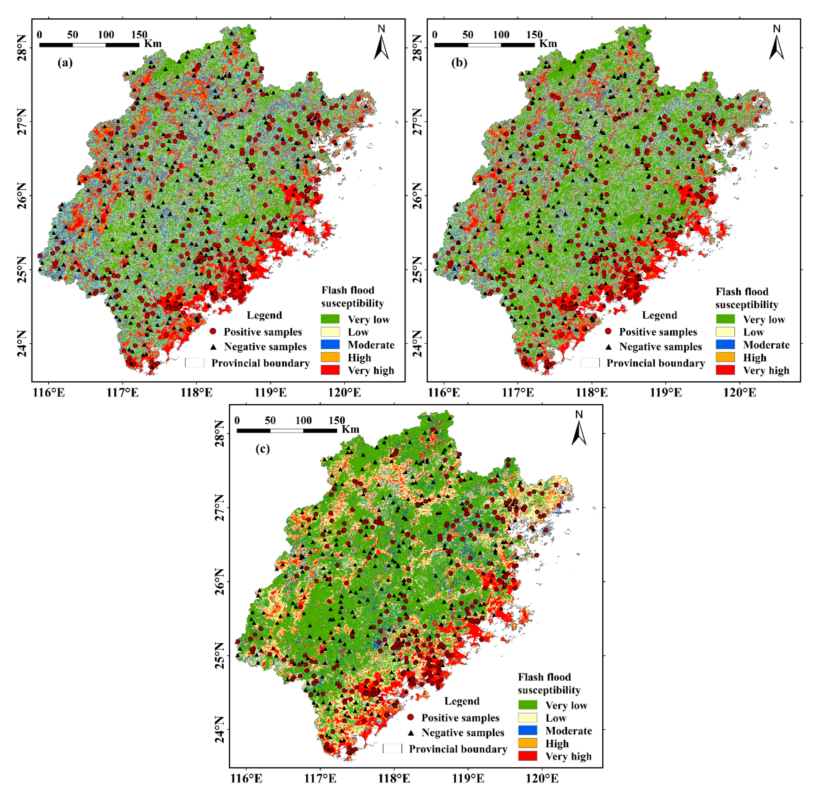
3.2.3. Flash Flood Susceptibility Maps

According to the natural break method, the values of the flash flood probability indexes P1, P2, and P3 were reclassified into five categories: very low, low, moderate, high, and very high. In addition, we calculated the average susceptibility value of each county. Most of the high and very high susceptibility level areas are located in the east, south, and southeast coastal areas, and in the north and west low mountain areas, which is consistent with the susceptibility map. Specifically, Dongshan County, the Longwen district, the Xiangcheng district; Jinmen County, Jinjiang City, Shishi City, the Licheng district, the Fengze district, Hui’an County, the Huli district, the Siming district, the Xiang’an district, the Xiuyu district, the Licheng district, Pingtan County, the Cangshan district, the Taijiang district, and the Gulou district have the highest susceptibility values, which indicates that these areas have the greatest possibility of flash flood occurrence in the future.

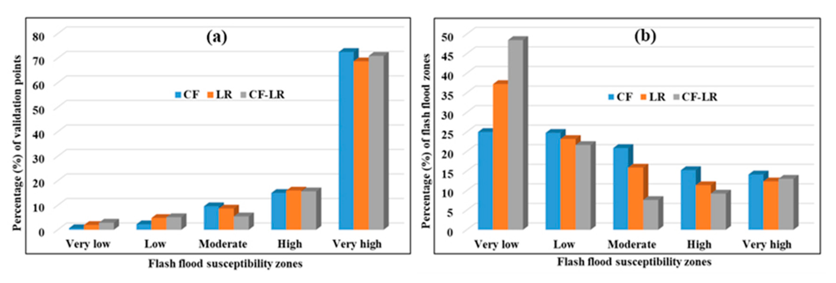
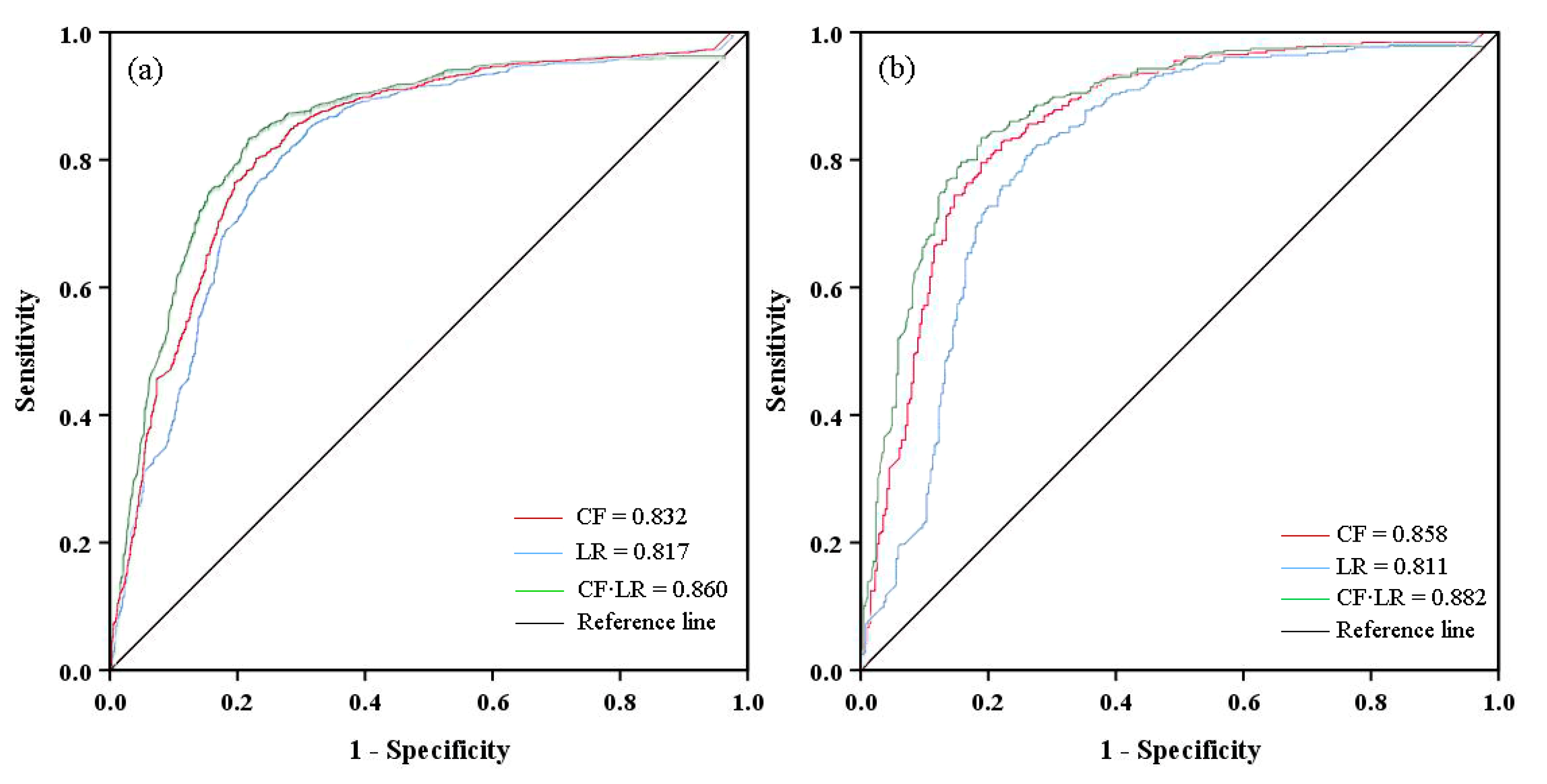
4. Validation of the Susceptibility Assessment Results and Comparison of the Different Models

Validation is very essential for the rationality of susceptibility zoning and the stability of the established model. Therefore, it is necessary to validate the rationality of the susceptibility zoning. On the one hand, the validation points (i.e., 20% of the actual historical flash flood points) and each flash flood susceptibility map were chosen for the overlay analysis. The results indicate that the distribution of the historical flash flood events is consistent with the susceptibility maps (Figure 4).
As can be seen from Figure 5a, for the CF model, 0.64%, 2.24%, 9.58%, 15.02%, and 72.52% of the validation points distributed in very low, low, moderate, high, and very high susceptibility levels. The validation point percentages for the LR model are 1.92%, 4.79%, 8.63%, 15.97%, and 68.69%, respectively, and those for the CF-LR model are 2.88%, 5.11%, 5.43%, 15.65%, and 70.93%, respectively. As can be seen from Figure 5b, for the CF model, the areas of each susceptibility level account for 24.99% (very low), 24.76% (low), 20.9% (moderate), 15.23% (high), and 14.12% (very high) of the total area of the study area. The percentages of the very low, low, moderate, high, and very high susceptibility areas for the LR model are 37.23%, 23.18%, 15.87%, 11.37%, and 12.34%, respectively, and those for the CF-LR model are 48.48%, 21.65%, 7.6%, 9.24%, and 13.03%, respectively. These results indicate that the CF and LR ensemble model overrated the area of the very low susceptibility level and underrated the area of the low, moderate, and high susceptibility levels, compared to the outputs of the standalone CF model and the standalone LR model. All three models estimated the area of the very high susceptibility level very approximately.
According to these three models, the number of validation points in the very high susceptibility level area accounts for the largest proportion of the total number of validation points, and the very low susceptibility level area accounts for the largest proportion of the total area of the study area, which meets the rationality validation standard of susceptibility zoning.
On the other hand, the receiver operating characteristic (ROC) curve was selected to assess the accuracy of the model. The x-coordinate of the ROC curve represents the true positive rate (1 − specificity), and the y-coordinate represents the false positive rate (sensitivity). The range of the area under ROC curve (AUC) is between 0 and 1, with larger values representing a more precise fit. In previous study [44], the AUC value was divided into four categories: weak (<0.6), moderate (0.6–0.7), good (0.7–0.8), and very good (>0.8). The success-rate and prediction-rate curves of the three models are shown in Figure 6a,b. The value of the success-rate curve of the CF-LR model is the maximum (0.860), and the value of the success rate for the LR model is the minimum value (0.817). The AUC for the prediction-rate curve represents the prediction ability of the model; the prediction rate was calculated using the 20% of the flash flood and non-flash flood points that were not used to establish the model. The AUC value of the prediction-rate curves for CF, LR, and CF-LR models are 0.858, 0.811, and 0.882, respectively. Therefore, the CF-LR model has the most precise prediction ability for the flash flood susceptibility map. In contrast, the LR model has the lowest prediction ability. Finally, the CF, LR, and CF-LR models demonstrated reliable prediction abilities in flash flood susceptibility assessment, but compared with the standalone CF and standalone LR models, the ensemble model has a greater flash flood prediction ability.

5. Discussion

The formation of flash floods is controlled by many factors, and it can never be completely predicted [59]. Thus, it is vitally important to choose appropriate assessment indicators, improve the prediction model, and improve the accuracy of susceptibility assessment results. Thus far, multiple flash flood susceptibility assessment methods have been developed by researchers around the world, and each of these models has its own advantages and disadvantages. For example, the lack of effective screening methods for the conditioning factors and the establishment of the model are relatively complex and depend on expert experience. It is worth noting that the model applied should be simple and highly efficient. Thus, in this research, PCC and Geodetector were used to screen the conditioning factors, and a combination of two different methods (CF and LR), along with a geographic information system (GIS) and remote sensing (RS), were used in the flash flood susceptibility assessment of Fujian Province, China. Ultimately, a more credible flash flood susceptibility map was created, which can be applied to provide more precise information for flood risk management.
For natural hazard susceptibility assessment, PCC was used to measure the correlation between the independent variable and with each other in a previous study [60]. However, they did not consider the correlation between the independent variable and the dependent variable. Although some studies have noticed this problem, they neglected the spatial pattern characteristics of the independent and dependent variables [17]. To address this problem, we utilized the PCC to screen the factors for which R < 0.8 and used Geodetector to screen the factors for which q > 0.05, from the 14 preliminary conditioning factors. From the results of the screening, H6_100, distance from rivers, slope, soil depth, soil type, and economic density were not selected as assessment indicators because they do not satisfy the two principles of R < 0.8 and q > 0.05. Ultimately, H24_100, annual rainfall, tropical cyclone index, elevation, topographic relief, NDVI, land use type, and population density were effective and selected as the final assessment indicators. This novel blended screening method not only overcomes the shortcomings of previous methods, but also makes the final assessment indicators more objective and accurate.
In the CF model, the calculation process is simple and easy to understand. For the CF method, the higher the CF value of a classification level, the greater the probability of a flash flood in this classification area. In terms of the CF values, the tropical cyclone index classification of 2–2.6, the annual rainfall classification of <1581.7 mm, the H24_100 classification 450–550mm, the elevation classification of <500 m, the topographic relief classification of <50 m, the land use classification of building land, the NDVI classification of <0.5, and the population density classification 2219.3–7463 people/km2 each have the highest CF values. In other words, the areas with these classifications are most prone to flash floods in the future. However, it should be noted that in some areas with high elevations or high topographic relief, the CF values are very low or even −1. The most likely reason for this is that these areas tend to be sparsely populated; thus, many historical flash flood events were not completely recorded in the early days of the founding of the People’s Republic of China [33].
The second method is LR, which has the main advantage of making full use of the information of every conditioning factor and determining the weight of each assessment indicator objectively. In this study, we connected the CF value of each assessment indicator to the training samples, and these values were used as the input data to train the model. Compared with the traditional standalone LR model, the CF-LR has a higher accuracy because in the standalone LR model the input training data are only the original value of the conditioning factor. Our study further corroborated the conclusions of Chen [61], Hong [62], and Jebur [18], which indicated that ensemble models result in better precision than single models. The outputs of the logistic regression analysis showed that land use, topographic relief, and H24_100 are the three main factors that significantly influence the formation of flash floods, while population density, annual rainfall, and the tropical cyclone index are the three factors that have the least influence on the formation of flash floods, which is consistent with the results of previous studies [32,63,64,65,66]. Generally speaking, the regions receiving higher rainfall with lower vegetation coverage and lower topographic relief are regarded as having a very high degree of susceptibility to flash floods [16]. In this study, an interesting finding was that as one of the rainfall indicators, H24_100 correlates with the formation of flash floods. However, as another rainfall indicator, the annual rainfall to some extent has an inhibitory effect on the formation of flash floods. The main reason for this result may be due to the obstruction of the atmospheric circulation by several mountain ranges; the areas of low-middle hills and the valley region in central Fujian are characterized by a distinct spatial distribution of annual rainfall [67,68]. Moreover, with acceleration of the global atmospheric water cycle [69] and some mountains affecting the movement of the southeastern monsoon, orographic rain is enhanced [70], thus giving rise to more frequent normal rainfall events than coastal regions [71]. Furthermore, inland areas have a lower population density than the coastal region, and this may have led to a lack of historical flash flood information for the more inland areas. In addition to these findings, this study also has certain limitations that are worth mentioning. First, topographic relief and elevation are two relatively important topographic factors affecting flash floods, but both elevation and topographic relief data were extracted from the ASTER GDEM instead of the LiDAR DEM, the latter having higher resolution that may influence the prediction results of the models. Therefore, it is suggested to use LiDAR rather than ASTER GDEM in future studies. Second, as the study area includes a variety of topographic features, we recommend that future studies investigate the flash flood susceptibilities of different physiognomy types to obtain more accurate prediction for flash flood prone areas. Third, the tropical cyclone index is also an important factor. However, Ref. [31] pointed out that tropical cyclones are indirect factors causing flash floods, and the real reason is the rainfall during the development and passage of tropical cyclones. This may be the main reason why the Beta value of the tropical cyclone index is small and negative. Therefore, in future studies, more accurate rainfall and rainfall accumulation indicators (e.g., maximum 6 h precipitation and initial soil moisture) should be selected.
The flash flood susceptibility maps obtained using the three models had a similar distribution pattern, but some differences were identified. Based on the results of the susceptibility maps, the very high susceptibility regions are mainly distributed in the eastern, southern, and southeastern parts of the province. This is generally consistent with the research results of Zhao [1] and Yue [72]. The population, industrial development, and urban expansion in these areas have been increasing at a very fast rate in recent years. These human activities have led to changes in land use and natural water bodies, which has significantly reduced the infiltration and discharge of flash floods. In addition, a large amount of sediment is deposited in the riverbed, which weakens the discharge capability, thereby leading to flash floods due to the river more easily overflowing its banks and causing damage to the buildings and farmland on both sides of the river [73]. Moreover, increasingly more land is being used for housing and infrastructure construction, and the urban drainage systems are underdeveloped, resulting in serious urban waterlogging. For these areas, our recommendations are as follows: (1) Insist on and enforce the “people-oriented” principle and improve people’s awareness of flash flood prevention; specifically, through a web page accessible to all people, post and diffuse information concerning flash flood susceptible regions and safe regions prior to construction [74]. (2) Build more sewers and drains in the cities. (3) Control human activities (e.g., the reasonable planning of land use and the prohibition of arbitrary deforestation). (4) Widen and clean watercourses. (5) Construct detention ponds.

6. Conclusions

The identification of flash flood susceptible areas is crucial for basin management, especially water resource management and flash flood risk reduction [75]. After identifying flash flood prone areas, both structural (“hard”) defenses and nonstructural (“soft”) measures can be suitably applied to mitigate flash flood damage [76]. In this study, we established an objective assessment indicator selection method, and used the CF, LR, and CF-LR models to prepare flash flood susceptibility maps of Fujian Province. We then evaluated the performances of the three models. The main conclusions of our study are summarized as follows.
(1) Based on the comprehensive application of the PCC and Geodetector, the selection of assessment indicators was more objective in that it improved the reliability of the assessment results.
(2) Land use, topographic relief, and 24 h precipitation (H24_100) with a 100-year return period have the most significant effect on the occurrence of flash floods in Fujian Province.
(3) The prediction abilities of the CF, LR, and CF- LR are very good, which is demonstrated by the fact that their AUC values are greater than 0.8. Moreover, the CF-LR model (0.882) had the highest AUC value, followed by the CF (0.858) and the LR model (0.811). In other words, in terms of the AUC value, the CF-LR has a 0.024–0.071 higher predictive ability than the CF and LR models.
(4) The high and very high susceptibility zones accounted for 22.27% to 29.35% of the total study area. Spatially, these areas are mainly located in the east, south, and southeast coastal areas and in the north and west low mountain areas.
Management organizations can combine our research results with the two-dimensional analysis results of numerical models such as the Hydrologic Engineering Center‘s (HEC) River Analysis System (HEC-RAS) in order to make more specific decisions on the prevention and control of flash floods in Fujian Province. Based on the excellent and very good accuracy of the susceptibility assessment method proposed in this study, it can be used in areas with similar environmental conditions and other natural disaster susceptibility analyses.

Author Contributions

Conceptualization, Yifan Cao and Hongliang Jia; formal analysis, Yifan Cao; data and resources, Junnan Xiong and Weiming Cheng; writing—original draft preparation, Yifan Cao and Junnan Xiong; writing—review and editing, Yifan Cao, Kun Li, Quan Pang, and Zhiwei Yong; supervision, Hongliang Jia and Weiming Cheng; funding acquisition, Junnan Xiong and Weiming Cheng. All authors have read and agreed to the published version of the manuscript.

Funding

This research was funded by Strategic Priority Research Program of the Chinese Academy of Sciences (Grant No. XDA20030302), Key R & D project of Sichuan Science and Technology Department (Grant No. 21QYCX0016), and the Science and Technology Project of Xizang Autonomous Region (Grant No. XZ201901-GA-07), National Flash Flood Investigation and Evaluation Project (Grant No. SHZH-IWHR-57), and Southwest Petroleum University of Science and Technology Innovation Team Projects (Grant No. 2017CXTD09).

Conflicts of Interest

The authors declare no conflict of interest.

References

  1. Zhao, G.; Pang, B.; Xu, Z.; Yue, J.; Tu, T. Mapping flood susceptibility in mountainous areas on a national scale in China. Sci. Total Environ. 2018, 615, 1133–1142. [Google Scholar] [CrossRef]
  2. Liu, Y.; Yang, Z.; Huang, Y.; Liu, C. Spatiotemporal evolution and driving factors of China’s flash flood disasters since 1949. Sci. China Earth Sci. 2018, 61, 1804–1817. [Google Scholar] [CrossRef]
  3. Liu, Y.; Yuan, X.; Guo, L.; Huang, Y.; Zhang, X. Driving Force Analysis of the Temporal and Spatial Distribution of Flash Floods in Sichuan Province. Sustainability 2017, 9, 1527. [Google Scholar] [CrossRef] [Green Version]
  4. Xiong, J.; Pang, Q.; Fan, C.; Cheng, W.; Ye, C.; Zhao, Y.; He, Y.-R.; Cao, Y. Spatiotemporal Characteristics and Driving Force Analysis of Flash Floods in Fujian Province. ISPRS Int. J. Geo-Inf. 2020, 9, 133. [Google Scholar] [CrossRef] [Green Version]
  5. Norbiato, D.; Borga, M.; Degli Esposti, S.; Gaume, E.; Anquetin, S. Flash flood warning based on rainfall thresholds and soil moisture conditions: An assessment for gauged and ungauged basins. J. Hydrol. 2008, 362, 274–290. [Google Scholar] [CrossRef]
  6. Ben Aissia, M.-A.; Chebana, F.; Ouarda, T.; Roy, L.; DesRochers, G.; Chartier, I.; Robichaud, É. Multivariate analysis of flood characteristics in a climate change context of the watershed of the Baskatong reservoir, Province of Québec, Canada. Hydrol. Process. 2012, 26, 130–142. [Google Scholar] [CrossRef] [Green Version]
  7. Oeurng, C.; Sauvage, S.; Sánchez-Pérez, J.-M. Assessment of hydrology, sediment and particulate organic carbon yield in a large agricultural catchment using the SWAT model. J. Hydrol. 2011, 401, 145–153. [Google Scholar] [CrossRef] [Green Version]
  8. Bahremand, A.; De Smedt, F.; Corluy, J.; Liu, Y.B.; Poorova, J.; Velcicka, L.; Kunikova, E. WetSpa Model Application for Assessing Reforestation Impacts on Floods in Margecany–Hornad Watershed, Slovakia. Water Resour. Manag. 2007, 21, 1373–1391. [Google Scholar] [CrossRef]
  9. Rahmati, O.; Pourghasemi, H.R.; Zeinivand, H. Flood susceptibility mapping using frequency ratio and weights-of-evidence models in the Golastan Province, Iran. Geocarto Int. 2016, 31, 42–70. [Google Scholar] [CrossRef]
  10. Papaioannou, G.; Vasiliades, L.; Loukas, A. Multi-Criteria Analysis Framework for Potential Flood Prone Areas Mapping. Water Resour. Manag. 2015, 29, 399–418. [Google Scholar] [CrossRef]
  11. Hong, H.; Tsangaratos, P.; Ilia, I.; Liu, J.; Zhu, A.-X.; Chen, W. Application of fuzzy weight of evidence and data mining techniques in construction of flood susceptibility map of Poyang County, China. Sci. Total Environ. 2018, 625, 575–588. [Google Scholar] [CrossRef] [PubMed]
  12. Chang, M.-J.; Chang, H.-K.; Chen, Y.-C.; Lin, G.-F.; Chen, P.-A.; Lai, J.-S.; Tan, Y.-C. A Support Vector Machine Forecasting Model for Typhoon Flood Inundation Mapping and Early Flood Warning Systems. Water 2018, 10, 1734. [Google Scholar] [CrossRef] [Green Version]
  13. Kia, M.B.; Pirasteh, S.; Pradhan, B.; Mahmud, A.R.; Sulaiman, W.N.A.; Moradi, A. An artificial neural network model for flood simulation using GIS: Johor River Basin, Malaysia. Environ. Earth Sci. 2012, 67, 251–264. [Google Scholar] [CrossRef]
  14. Wang, Z.; Lai, C.; Chen, X.; Yang, B.; Zhao, S.; Bai, X. Flood hazard risk assessment model based on random forest. J. Hydrol. 2015, 527, 1130–1141. [Google Scholar] [CrossRef]
  15. Bui, D.T.; Khosravi, K.; Shahabi, H.; Daggupati, P.; Adamowski, J.F.; Melesse, A.M.; Pham, B.T.; Pourghasemi, H.R.; Mahmoudi, M.; Bahrami, S.; et al. Flood Spatial Modeling in Northern Iran Using Remote Sensing and GIS: A Comparison between Evidential Belief Functions and Its Ensemble with a Multivariate Logistic Regression Model. Remote Sens. 2019, 11, 1589. [Google Scholar] [CrossRef] [Green Version]
  16. Tehrany, M.S.; Pradhan, B.; Jebur, M.N. Spatial prediction of flood susceptible areas using rule based decision tree (DT) and a novel ensemble bivariate and multivariate statistical models in GIS. J. Hydrol. 2013, 504, 69–79. [Google Scholar] [CrossRef]
  17. Yang, J.; Song, C.; Yang, Y.; Xu, C.; Guo, F.; Xie, L. New method for landslide susceptibility mapping supported by spatial logistic regression and GeoDetector: A case study of Duwen Highway Basin, Sichuan Province, China. Geomorphology 2019, 324, 62–71. [Google Scholar] [CrossRef]
  18. Jebur, M.N.; Pradhan, B.; Tehrany, M.S. Optimization of landslide conditioning factors using very high-resolution airborne laser scanning (LiDAR) data at catchment scale. Remote Sens. Environ. 2014, 152, 150–165. [Google Scholar] [CrossRef]
  19. Lee, S.; Talib, J.A. Probabilistic landslide susceptibility and factor effect analysis. Environ. Earth Sci. 2005, 47, 982–990. [Google Scholar] [CrossRef]
  20. Zeng, F.; Lai, C.; Wang, Z. Flood Risk Assessment Based on Principal Component Analysis for Dongjiang River Basin. In Proceedings of the 2012 2nd International Conference on Remote Sensing, Environment and Transportation Engineering, South China University of Technology, Guangzhou, China, 1–3 June 2012; pp. 1–4. [Google Scholar]
  21. Shahabi, H.; Bui, D.T.; Yunus, A.P.; Jia, K.; Song, X.; Revhaug, I.; Xia, H.; Zhu, Z. Optimization of Causative Factors for Landslide Susceptibility Evaluation Using Remote Sensing and GIS Data in Parts of Niigata, Japan. PLoS ONE 2015, 10, e0133262. [Google Scholar] [CrossRef] [Green Version]
  22. Pourghasemi, H.R.; Mohammady, M.; Pradhan, B. Landslide susceptibility mapping using index of entropy and conditional probability models in GIS: Safarood Basin, Iran. Catena 2012, 97, 71–84. [Google Scholar] [CrossRef]
  23. Luo, W.; Liu, C.-C. Innovative landslide susceptibility mapping supported by geomorphon and geographical detector methods. Landslides 2018, 15, 465–474. [Google Scholar] [CrossRef]
  24. Wang, J.; Xu, C. Geodetector: Principle and prospective. Acta Geogr. Sin. 2017, 72, 116–134. [Google Scholar]
  25. Zhu, L.; Meng, J.; Zhu, L. Applying Geodetector to disentangle the contributions of natural and anthropogenic factors to NDVI variations in the middle reaches of the Heihe River Basin. Ecol. Indic. 2020, 117, 106545. [Google Scholar] [CrossRef]
  26. Wang, X.F.; Zhang, Y.W.; Ma, J.J. Factors influencing the incidence of bacterial dysentery in parts of southwest China, using data from the geodetector. Chin. J. Epidemiol. 2019, 40, 953–959. [Google Scholar]
  27. China Statistical Yearbook. 2018. Available online: http://tjj.fujian.gov.cn/tongjinianjian/dz2018/index-cn.htm (accessed on 30 November 2020).
  28. Zhang, K.; Hong, W.; Wu, C.; Ding, X. Study on the Spatial Pattern of Rainfall Erosivity Based on Geostatistics and GIS of Fujian Province. J. Mt. Sci. 2009, 27, 5344–5385. [Google Scholar]
  29. Fujian Bureau of Geology and Mineral Resources. Regional Geology of Fujian Province; Geological Publishing House: Beijing, China, 1985. [Google Scholar]
  30. Wang, D.; Zhou, X. Volcanic Petrology; Science Press: Beijing, China, 1982. [Google Scholar]
  31. Nandi, A.; Mandal, A.; Wilson, M.; Smith, D. Flood hazard mapping in Jamaica using principal component analysis and logistic regression. Environ. Earth Sci. 2016, 75, 1–16. [Google Scholar] [CrossRef]
  32. Tehrany, M.S.; Shabani, F.; Jebur, M.N.; Hong, H.; Chen, W.; Xie, X. GIS-based spatial prediction of flood prone areas using standalone frequency ratio, logistic regression, weight of evidence and their ensemble techniques. Geomat. Nat. Hazards Risk 2017, 8, 1538–1561. [Google Scholar] [CrossRef]
  33. Xiong, J.; Ye, C.; Cheng, W.; Guo, L.; Zhou, C.; Zhang, X. The Spatiotemporal Distribution of Flash Floods and Analysis of Partition Driving Forces in Yunnan Province. Sustainability 2019, 11, 2926. [Google Scholar] [CrossRef] [Green Version]
  34. Yuan, X.; Liu, Y.; Huang, Y.; Tian, F. An approach to quality validation of large-scale data from the Chinese Flash Flood Survey and Evaluation (CFFSE). Nat. Hazards 2017, 89, 693–704. [Google Scholar] [CrossRef]
  35. Su, C.; Tian, Q.; Liu, B.; Yang, G.; Huang, K.; Huang, F. Regional Landslide Susceptibility Assessment for Longnan County in Jiangxi Province. Sci. Technol. Eng. 2019, 19, 919. [Google Scholar]
  36. Tehrany, M.S.; Kumar, L. The application of a Dempster–Shafer-based evidential belief function in flood susceptibility mapping and comparison with frequency ratio and logistic regression methods. Environ. Earth Sci. 2018, 77, 490. [Google Scholar] [CrossRef]
  37. Youssef, A.M.; Pradhan, B.; Hassan, A.M. Flash flood risk estimation along the St. Katherine road, southern Sinai, Egypt using GIS based morphometry and satellite imagery. Environ. Earth Sci. 2011, 62, 611–623. [Google Scholar] [CrossRef]
  38. Xiong, J.; Li, J.; Cheng, W.; Zhou, C.; Guo, L.; Zhang, X.; Wang, N.; Li, W. Spatial-temporal distribution and the influencing factors of mountain flood disaster in southwest China. Acta Geogr. Sin. 2019, 74, 1374–1391. [Google Scholar]
  39. Slater, L.J.; Singer, M.B.; Kirchner, J.W. Hydrologic versus geomorphic drivers of trends in flood hazard. Geophys. Res. Lett. 2015, 42, 370–376. [Google Scholar] [CrossRef] [Green Version]
  40. Bui, D.T.; Pradhan, B.; Nampak, H.; Bui, Q.-T.; Tran, Q.-A.; Nguyen, Q.-P. Hybrid artificial intelligence approach based on neural fuzzy inference model and metaheuristic optimization for flood susceptibilitgy modeling in a high-frequency tropical cyclone area using GIS. J. Hydrol. 2016, 540, 317–330. [Google Scholar] [CrossRef]
  41. Meraj, G.; Romshoo, S.A.; Yousuf, A.R.; Altaf, S.; Altaf, F. Assessing the influence of watershed characteristics on the flood vulnerability of Jhelum basin in Kashmir Himalaya. Nat. Hazards 2015, 77, 1531–1575. [Google Scholar] [CrossRef]
  42. Cai, D.; Xiao, X.; Sun, J. Assessment of the Difficulty of Warning Mountain Torrent Disasters: Case Study of the Yangtze River. J. Yangtze River Sci. Res. Inst. 2015, 32, 848. [Google Scholar]
  43. Toosi, A.S.; Calbimonte, G.H.; Nouri, H.; Alaghmand, S. River basin-scale flood hazard assessment using a modified multi-criteria decision analysis approach: A case study. J. Hydrol. 2019, 574, 660–671. [Google Scholar] [CrossRef]
  44. Choubin, B.; Moradi, E.; Golshan, M.; Adamowski, J.; Sajedi-Hosseini, F.; Mosavi, A. An ensemble prediction of flood susceptibility using multivariate discriminant analysis, classification and regression trees, and support vector machines. Sci. Total Environ. 2019, 651, 2087–2096. [Google Scholar] [CrossRef]
  45. Shangguan, W.Y.; Dai, B.; Liu, A.; Zhu, Q.; Duan, L.; Wu, D.; Ji, A.; Ye, H.; Yuan, Q.; Zhang, D.; et al. A China Dataset of Soil Properties for Land Surface Modeling. J. Adv. Model. Earth Syst. 2013, 5, 212–224. [Google Scholar] [CrossRef]
  46. Vojtek, M.; Vojteková, J. Flood Susceptibility Mapping on a National Scale in Slovakia Using the Analytical Hierarchy Process. Water 2019, 11, 364. [Google Scholar] [CrossRef] [Green Version]
  47. Li, H.; Wan, Q. Study on Rainfall Index Selection for Hazard Analysis of Mountain Torrents Disaster of Small Watersheds. J. Geo-Inf. Sci. 2017, 19, 425–435. [Google Scholar]
  48. Ding, M.; Heiser, M.; Hübl, J.; Fuchs, S. Regional vulnerability assessment for debris flows in China—A CWS approach. Landslides 2016, 13, 537–550. [Google Scholar] [CrossRef]
  49. Luo, W.; Jasiewicz, J.; Stepinski, T.F.; Wang, J.; Xu, C.; Cang, X. Spatial association between dissection density and environmental factors over the entire conterminous United States. Geophys. Res. Lett. 2016, 43, 692–700. [Google Scholar] [CrossRef] [Green Version]
  50. Xiong, J.; Li, W.; Cheng, W.; Fan, C.; Li, J.; Zhao, Y. Spatial variability and influencing factors of LST in plateau area: Exemplified by Sangzhuzi District. Remote Sens. Land Resour. 2019, 31, 1641–1671. [Google Scholar]
  51. Wang, J.-F.; Zhang, T.-L.; Fu, B. A measure of spatial stratified heterogeneity. Ecol. Indic. 2016, 67, 250–256. [Google Scholar] [CrossRef]
  52. Chen, Z.; Liang, S.; Ke, Y.; Yang, Z.; Zhao, H. Landslide susceptibility assessment using evidential belief function, certainty factor and frequency ratio model at Baxie River basin, NW China. Geocarto Int. 2017, 34, 348–367. [Google Scholar] [CrossRef]
  53. Arabameri, A.; Pradhan, B.; Rezaei, K. Gully erosion zonation mapping using integrated geographically weighted regression with certainty factor and random forest models in GIS. J. Environ. Manag. 2019, 232, 928–942. [Google Scholar] [CrossRef]
  54. Chen, W.; Li, W.; Chai, H.; Hou, E.; Li, X.; Ding, X. GIS-based landslide susceptibility mapping using analytical hierarchy process (AHP) and certainty factor (CF) models for the Baozhong region of Baoji City, China. Environ. Earth Sci. 2015, 75, 1–14. [Google Scholar] [CrossRef] [Green Version]
  55. Chen, X.; Chen, H.; You, Y.; Chen, X.; Liu, J. Weights-of-evidence method based on GIS for assessing susceptibility to debris flows in Kangding County, Sichuan Province, China. Environ. Earth Sci. 2016, 75, 1–16. [Google Scholar] [CrossRef]
  56. Lim, J.; Lee, K.-S. Flood Mapping Using Multi-Source Remotely Sensed Data and Logistic Regression in the Heterogeneous Mountainous Regions in North Korea. Remote Sens. 2018, 10, 1036. [Google Scholar] [CrossRef] [Green Version]
  57. Trigila, A.; Iadanza, C.; Esposito, C.; Mugnozza, G.S. Comparison of Logistic Regression and Random Forests techniques for shallow landslide susceptibility assessment in Giampilieri (NE Sicily, Italy). Geomorphology 2015, 249, 119–136. [Google Scholar] [CrossRef]
  58. Chauhan, S.; Sharma, M.; Arora, M. Landslide susceptibility zonation of the Chamoli region, Garhwal Himalayas, using logistic regression model. Landslides 2010, 7, 411–423. [Google Scholar] [CrossRef]
  59. Khosravi, K.; Khosravi, K.; Pham, B.T.; Adamowski, J.; Dou, J.; Pradhan, B.; Shahabi, H.; Ly, H.-B.; Gróf, G.; Ho, H.L.; et al. A comparative assessment of flood susceptibility modeling using Multi-Criteria Decision-Making Analysis and Machine Learning Methods. J. Hydrol. 2019, 573, 311–323. [Google Scholar] [CrossRef]
  60. Al-Juaidi, A.E.M.; Nassar, A.M.; Al-Juaidi, O.E.M. Evaluation of flood susceptibility mapping using logistic regression and GIS conditioning factors. Arab. J. Geosci. 2018, 11, 765. [Google Scholar] [CrossRef]
  61. Chen, W.; Shahabi, H.; Zhang, S.; Khosravi, K.; Shirzadi, A.; Chapi, K.; Pham, B.T.; Han, L.; Chai, H.; Ma, J.; et al. Landslide Susceptibility Modeling Based on GIS and Novel Bagging-Based Kernel Logistic Regression. Appl. Sci. 2018, 8, 2540. [Google Scholar] [CrossRef] [Green Version]
  62. Hong, H.; Liu, J.; Zhu, A.-X.; Shahabi, H.; Pham, B.T.; Chen, W.; Pradhan, B.; Bui, D.T. A novel hybrid integration model using support vector machines and random subspace for weather-triggered landslide susceptibility assessment in the Wuning area (China). Environ. Earth Sci. 2017, 76, 652. [Google Scholar] [CrossRef]
  63. Liuzzo, L.; Sammartano, V.; Freni, G. Comparison between Different Distributed Methods for Flood Susceptibility Mapping. Water Resour. Manag. 2019, 33, 3155–3173. [Google Scholar] [CrossRef]
  64. Adiat, K.; Nawawi, M.; Abdullah, K. Assessing the accuracy of GIS-based elementary multi criteria decision analysis as a spatial prediction tool–A case of predicting potential zones of sustainable groundwater resources. J. Hydrol. 2012, 440, 75–89. [Google Scholar] [CrossRef]
  65. Mind’Je, R.; Li, L.; Amanambu, A.C.; Nahayo, L.; Nsengiyumva, J.B.; Gasirabo, A.; Mindje, M. Flood susceptibility modeling and hazard perception in Rwanda. Int. J. Disaster Risk Reduct. 2019, 38, 101211. [Google Scholar] [CrossRef]
  66. Tehrany, M.S.; Kumar, L.; Jebur, M.N.; Shabani, F. Evaluating the application of the statistical index method in flood susceptibility mapping and its comparison with frequency ratio and logistic regression methods. Geomat. Nat. Hazards Risk 2018, 10, 79–101. [Google Scholar] [CrossRef]
  67. Huang, Y.; Duan, Y.; Yu, H. A Study of the Impact of Terrain on the Precipitation of “KROSA”. Meteorol. Mon. 2009, 9, 2. [Google Scholar]
  68. Pang, M.; Si, G. Influence of The Regional Scale Topography on the Climatalogical Distribution of Precipitatio Over Southeastern China. J. Trop. Meteorol. 1993, 9, 370–374. [Google Scholar]
  69. Xue, D.; Lu, J.; Leung, L.R.; Zhang, Y. Response of the Hydrological Cycle in Asian Monsoon Systems to Global Warming Through the Lens of Water Vapor Wave Activity Analysis. Geophys. Res. Lett. 2018, 45, 11904. [Google Scholar] [CrossRef]
  70. Zhang, H.; Sun, J.; Xiong, J. Spatial-Temporal Patterns and Controls of Evapotranspiration across the Tibetan Plateau (2000–2012). Adv. Meteorol. 2017, 2017, 7082606. [Google Scholar] [CrossRef] [Green Version]
  71. King, A.D.; Donat, M.G.; Fischer, E.M.; Hawkins, E.; Alexander, L.V.; Karoly, D.J.; Dittus, A.J.; Lewis, S.C.E.; Perkins, S. The timing of anthropogenic emergence in simulated climate extremes. Environ. Res. Lett. 2015, 10, 094015. [Google Scholar] [CrossRef]
  72. Yue, Q.; Zhang, L.; Liu, C.; Zhang, H. GIS-based Risk Zoning of Flood Disasters in Upstream of the Minjiang River. J. Environ. Eng. Technol. 2015, 5, 2932–2998. [Google Scholar]
  73. Keesstra, S.; Nunes, J.P.; Saco, P.M.; Parsons, A.J.; Poeppl, R.; Masselink, R.; Cerdà, A. The way forward: Can connectivity be useful to design better measuring and modelling schemes for water and sediment dynamics? Sci. Total Environ. 2018, 644, 1557–1572. [Google Scholar] [CrossRef]
  74. Ramesh, V.; Iqbal, S.S. Urban flood susceptibility zonation mapping using evidential belief function, frequency ratio and fuzzy gamma operator models in GIS: A case study of Greater Mumbai, Maharashtra, India. Geocarto Int. 2020, 1–26. [Google Scholar] [CrossRef]
  75. Mahmood, S.; Rahman, A.-U. Flash flood susceptibility modeling using geo-morphometric and hydrological approaches in Panjkora Basin, Eastern Hindu Kush, Pakistan. Environ. Earth Sci. 2019, 78, 43. [Google Scholar] [CrossRef]
  76. Kundzewicz, Z.; Su, B.; Wang, Y.; Xia, J.; Huang, J.; Jiang, T. Flood risk and its reduction in China. Adv. Water Resour. 2019, 130, 37–45. [Google Scholar] [CrossRef]
Figure 1. The study area: (a) the geographical position of Fujian Province in China, (b) the elevation of Fujian Province, and (c) the distribution of flash floods in Fujian Province.
Ijgi 09 00748 g001
Figure 2. (a) Flash flood density of Fujian Province and (b) the q-statistic indices calculated by Geodetector.
Ijgi 09 00748 g002
Figure 3. Eight assessment indicators: (a) H24_100, (b) annual rainfall, (c) tropical cyclone index, (d) elevation, (e) topographic relief, (f) NDVI, (g) land use type, and (h) population density.
Ijgi 09 00748 g003
Figure 4. Flash flood susceptibility map produced using the (a) CF, (b) LR, and (c) CF-LR models.
Ijgi 09 00748 g004
Figure 5. A histogram showing the percentages of (a) the validation points and (b) the flash flood zones obtained using the three models.
Ijgi 09 00748 g005
Figure 6. The success-rate and prediction-rate curves for the flash flood map: (a) success rate and (b) prediction rate.
Ijgi 09 00748 g006
Table 1. Sources and types of raw datasets.
FactorsSubfactorsSource, Resolution, and Type
Flash flood inventory mapHistorical flash flood pointsFlash Flood Investigation and Evaluation Dataset of China (FFIEDC), 1:50,000, vector data
PrecipitationH6_100FFIEDC, vector data
H24_100FFIEDC, vector data
Annual rainfallNational Meteorological Information Center. (http://data.cma.cn/), table data
Tropical cycloneTropical cyclone indexAn overview of the China Meteorological Administration’s tropical cyclone database (tcdata.typhoon.org.cn), text data
Digital elevation modelElevationGeospatial Data Cloud (www.gscloud.cn), 30 m × 30 m, raster data
Slope
Topographic relief
SoilSoil typeFFIEDC, vector data
Soil depthA China Dataset of Soil Properties for Land Surface Modeling, 1 km × 1 km, raster data
Land useLand use typeFFIEDC, vector data
VegetationsNDVINational Earth System Science Data Center (http://www.geodata.cn/), 1 km × 1 km, raster data
River systemDistance from riversFFIEDC, vector data
Human activitiesPopulation densityResource and Environment Data Center (RESDC), Chinese Academy of Sciences (http://www.resdc.cn/), 1 km × 1 km, raster data
Economic density
Table 2. The Pearson correlation coefficient (PCC) value (R) and corresponding correlation levels.
Value of PCC (R)Correlation Levels
|R| = 0No correlation
0 < |R| < 0.2Very weak correlation
0.2 < |R| < 0.4Weak correlation
0.4 < |R| < 0.6Intermediate correlation
0.6 < |R| < 0.8Strong correlation
0.8 < |R| < 1Very strong correlation
|R| = 1Perfect correlation
Table 3. Correlation matrix of the conditioning factors.
X1X2X3X4X5X6X7X8X9X10X11X12X13X14
X11
X2−0.651
X30.81−0.631
X4−0.420.35−0.381
X5−0.320.47−0.320.261
X6−0.180.31−0.170.130.31
X7−0.220.41−0.20.110.450.681
X80.27−0.280.29−0.38−0.23−0.1−0.041
X9−0.020.11−0.050.020.250.060.07−0.051
X10−0.190.25−0.110.120.220.260.34−0.050.041
X11−0.10.17−0.070.02−0.070.040.05−0.030.010.061
X120.3−0.390.28−0.23−0.37−0.21−0.280.19−0.05−0.16−0.281
X130.43−0.380.42−0.23−0.31−0.15−0.140.64−0.05−0.13−0.110.31
X140.42−0.360.41−0.31−0.29−0.12−0.090.7−0.04−0.12−0.080.260.921
Notes: X1—economic density, X2—normalized difference vegetation index (NDVI), X3—population density, X4—annual rainfall, X5—elevation, X6—slope, X7—topographic relief, X8—tropical cyclone index, X9—distance from rivers, X10—land use type, X11—soil depth, X12—soil type, X13—H6_100, X14—H24_100.
Table 4. CF values of the assessment indicators.
FactorClassFlash FloodCFFactorClassFlash FloodCF
Tropical cyclone index<1.4180−0.49Topographic relief (m)<5012400.76
1.4–2662−0.1350–100246−0.54
2–2.66150.41100–15061−0.87
2.6–3.21080.31150–20017−0.92
>3.21−0.88200–3002−0.97
Annual rainfall (mm)<1581.74650.53>3000−1
1581.7–1649.33660.07Land use typeGrassland58−0.52
1649.3–1712.8221−0.4Farmland7310.57
1712.9–1778.4237−0.3Building land5020.93
>1778.4277−0.08Forest land186−0.82
H24_100 (mm)<250125−0.42Brushland2−0.57
250–350561−0.34Water conservancy facilities740.75
350–4507100.37Water area3−0.34
450–5501570.74Marshland50.62
>550130.11Other land50.65
Elevation (m)<50013440.36Population density
(people/km2)
<410.9930−0.3
500–1000212−0.65411–2219.25130.58
1000–150010−0.892219.3–74631230.86
1500–20000−17463.1–14,515.10−1
>20000−1>14,515.10−1
NDVI<0.51890.84
0.5–0.643080.78
0.64–0.743700.59
0.74–0.8493−0.01
>0.8206−0.75
Table 5. The results of the logistic regression analysis.
FactorBetaWaldSigExp(B)
Tropical cyclone index−0.1160.2670.0150.891
Annual rainfall−0.2755.0540.0250.759
H24_1000.5355.680.0171.707
Elevation0.4210.4610.0011.521
Topographic relief1.087156.83502.965
Land use type1.107186.56603.024
NDVI0.48915.90401.631
Population density−0.3493.2320.0020.705
B−0.1446.0920.0140.866
Publisher’s Note: MDPI stays neutral with regard to jurisdictional claims in published maps and institutional affiliations.

