Geographic Information System Technology Combined with Back Propagation Neural Network in Groundwater Quality Monitoring

School of Earth Sciences and Resources, China University of Geosciences, Beijing 100000, China
*
Author to whom correspondence should be addressed.
ISPRS Int. J. Geo-Inf. 2020, 9(12), 736; https://doi.org/10.3390/ijgi9120736
Submission received: 14 October 2020
/
Revised: 20 November 2020
/
Accepted: 4 December 2020
/
Published: 9 December 2020
(This article belongs to the Special Issue The Use of GIS and Soft Computing Methods in Water Resource Planning)
Abstract
:This study was conducted to explore the distribution and changes of groundwater resources in the research area, and to promote the application of geographic information system (GIS) technology and its deep learning methods in chemical type distribution and water quality prediction of groundwater. The Shiyang River Basin in Minqin County was selected as the research object for analyzing the natural components distribution and its preliminary forecast in partial areas. With the priority control of groundwater pollutants, the concentration changes of four indicators (including the permanganate index) in different spatial distributions were analyzed based on the GIS technology, so as to provide a basis for the groundwater quality prediction. Taking the permanganate as a benchmark, this study evaluated the prediction effects of the conventional back propagation (BP) neural network (BPNN) model and the optimized BPNN based on the golden section (GBPNN) and wavelet transform (WBPNN). The algorithm proposed in this study is compared with several classic prediction algorithms for analysis. Groundwater quality level and distribution rules in the research area are evaluated with the proposed algorithm and GIS technology. The results reveal that GIS technology can characterize the spatial concentration distribution of natural indicators and analyze the chemical distribution of groundwater quality based on it. In contrast, the WBPNN has the best prediction result. Its average error of the whole process is 3.66%, and the errors corresponding to the six predicated values are all below 10%, which is dramatically better than the values of the other two models. The maximal prediction accuracy of the proposed algorithm is 97.68%, with an average accuracy of 96.12%. The prediction results on the water quality level are consistent with the actual condition, and the spatial distribution rules of the groundwater water quality can be shown clearly with the GIS technology combined with the proposed algorithm. Therefore, it is of great significance to explore the distribution and changes of regional groundwater quality, and this studywill play a critical role in determining the groundwater quality.
1. Introduction
As the source of life, water is an extremely important resource in daily production and human life, as well as a critical environmental resource that ensures stable survival of various organisms on the earth [1,2]. Groundwater specifically refers to the water located in the crevices of the geological body. As a widespread water type with many excellent properties, groundwater is also an indispensable and significant component of water resources, and it is especially critical for arid or semi-arid regions. At the same time, groundwater becomes an alternative resource when the surface water pollution is severe or aggravated, and its essential role under such conditions is self-evident [3,4]. However, the unreasonable utilization of groundwater has caused many ecological problems in recent years. As a result, the investigation of water quality monitoring and water quality distribution rules is also of great significance for promoting the reasonable utilization of groundwater resources.
Currently, many researchers are working on groundwater resource monitoring and water quality assessment. Taking the Daya Bay as the research object, Kai et al. analyzed and evaluated the water quality of the area through analysis of the changes in the concentration of some major elements including dissolved inorganic phosphorus and silicate, and analyzed and discussed the transfer of groundwater based on the numerical simulation of groundwater flow [5]; Mohana and Velmurugan adopted Gibb’s diagram to evaluate the change mechanism of the chemical composition of the groundwater, revealed the uniqueness of groundwater based on the relationship among the main ions, assessed the hydro-chemical characteristics of the physical and chemical parameters related to groundwater through contour maps, and determined the important geochemical characteristics of groundwater quality evaluation and the influences of monsoon changes on the chemical composition of groundwater [6]; Ostad–Ali-Askari (2017) studied the nitrate pollution of groundwater, and modeled and estimatedthe nitrate pollution of groundwater at the edge of a river in a certain region through the use of water quality and artificial neural network (ANN),concluding after repeated experiments that the network having a hidden layer and 19 neurons had the smallest error in the training, testing, and verification, and the ANN can be applied to the study of water quality parameters [7]; Zanotti (2019) evaluated the quality of groundwater and surface water with the positive matrix decomposition method, thereby determining the key hydrological characteristics and processes for regulation, and found that this method had strong interaction between groundwater and surface water and was applicable in the hydrological system greatly affected by the agricultural activities [8]; Johnny (2018) analyzed the spatial distribution of groundwater by using the inverse distance weight (IDW)-based on geographic information system (GIS) and explored the rationality of groundwater for drinking and irrigation [9]. Therefore, there are many research results on groundwater quality monitoring, and some researches are related to the application of neural network methods and GIS technology. However, there are few studies on the application of the optimized neural network and combination of GIS and neural network algorithms in groundwater monitoring or quality assessment.
Based on this, GIS technology was applied to the analysis of the spatial distribution of groundwater pollutants, and the BPNN method was applied to the monitoring of groundwater quality for better analyzing the groundwater quality in the downstream areas such as Shiyang River in Minqin County. Based on a combination of GIS technology and BPNN method, it is expected to provide a feasible idea and method for monitoring the distribution of groundwater pollutants and water quality. The spatial distribution of groundwater was analyzed and discussed based on the water chemical characteristics of the research area, and the spatial distribution of groundwater was analyzed with the GIS technology. Based on the water chemical characteristics and spatial distribution of the groundwater in the research area, the groundwater was predicted using the neural network method based on the deep learning to provide a reliable reference for determining the groundwater quality level. During the prediction of groundwater, the golden section and wavelet transform were introduced to improve and optimize the back propagation (BP) neural network(BPNN) into wavelet transform (WBPNN) and golden section (GBPNN). The GBPNN was applied to water quality prediction. This is a manifestation of the research that is different from others in related fields. This study creatively proposes the GBPNN algorithm and WBPNN algorithm, and the latter can achieve better prediction results than other classic prediction algorithms.
In summary, this study analyzed the groundwater quality monitoring and spatial distribution through the combination of GIS technology and BPNN method; it was found that the golden section and wavelet transform can significantly improve the predictive performance of BPNN after the BPNN is optimized.
2. Materials and Methods
2.1. Overview of GIS and Research Area
GIS is a tool for spatial data analysis and processing. The earliest application of this system was in the management of water resources. With the rapid development of computer information technology in recent years, the development of GIS in the field of hydrology has become a key focus of the society [10,11]. Specifically, the development of GIS technology is accompanied by the integration of remote sensing and mapping, space technology, and computer information technology. GIS can not only search for relevant spatial data information, but also collect and analyze the image data information. In addition, GIS can analyze and process the spatial data information, which is its biggest feature in contrast to other data analysis systems [12].
Considering the important role of groundwater in arid or semi-arid regions, the Shiyang River Basin in Minqin County in northeast of the Hexi Corridor of Gansu Province was selected as the research object in this study for exploration and analysis. From a climatic point of view, it is located in a temperate arid desert climate zone, which has a typical arid continental climate with obvious characteristics of low precipitation and large evaporation. The temperature difference between morning and evening is large, and the difference between the highest and the lowest temperature sometimes even reaches about 60 °C. At the same time, it has abundant light source resources, and its evaporation is greatly affected by soil salinization and diving mineralization. It can be considered as one of the driest areas in the country. From a hydrogeological point of view, its groundwater storage mainly includes two parts: bedrock fracture water and interstitial water. Based on the different properties of aquifers, bedrock fracture water and interstitial water can be divided into different levels [13]. For example, the interstitial water can be divided into phreatic confined water, deep confined water, and aquifers with different locations. The groundwater level has been greatly reduced due to the over-extraction of groundwater in the past few decades, which has led to the degradation of vegetation in the area. In addition, the continuous increase in groundwater salinity has led toaggravation of soil salinization and desertification, which has accelerated the growth of some xerophytes. Since the 1970s, the basin area in Minqin County has been continuously exploiting groundwater resources, and the surface water resources have been in short supply, so groundwater resources in the region decreased gradually, which in turn led to a series of social and environmental problems. In general, the current main problems of groundwater in Minqin County include serious over-exploitation, deterioration of groundwater quality, and a drop in groundwater level [14]. The geographical location of the study area is shown in Figure 1 below.
Based on the existing problems of groundwater in Minqin, it is essential to predict the groundwater quality and analyze and discuss the distribution of groundwater in this region. Based on abovementioned contents, the water chemical characteristics of the research area were analyzed; the spatial distribution of related water chemical elements was discussed by relying on GIS spatial interpolation technology; and the BPNN method was introduced to evaluate the prediction of groundwater quality [15]. The spatial distribution of different water quality levels in the research area can be obtained based on the GIS technology. The prediction of the spatial distribution and water quality of groundwater play an important role in determining the level of groundwater pollution.
2.2. Analysis of the Temporal and Spatial Evolution of Water Chemical Types
The dynamic evolution of regional groundwater quality was analyzed from time and space aspects. Based on the water chemical information data obtained through actual monitoring of the research area, 2010, 2015, and 2019 were selected as the study years. April was selected for analysis taking into account the impact of seasonal changes. The distribution of spatial interpolation sites in the selected research area under different representative years is shown in Figure 2 below.
The spatial interpolation maps for the key influencing factors affecting the groundwater quality are made under the ArsGis platform. The supply of groundwater in the research area is mainly derived from the recharge of underground runoff, and the groundwater mainly flows from south to north. According to the specific locations of the selected observation wells, water samples were collected from six observation wells, including 176 Hongyashan Reservoir, 167 Xuebai Village, 159 Dam, 142 Datan, 132 Hongshaliang, and 112 West Canal. The key chemical elements in the research area change with the content of the groundwater flow upwards, and the spatial change rules were analyzed by linear fitting. In this way, the proposed method can lay a foundation for groundwater quality prediction and spatial grade distribution analysis.
2.3. Back Propagation Neural Network
Among the many neural network models of deep learning, ANN relies on the information transmission among multiple neurons to realize the analysis and processing of complex data [16]. Through the learning process in the external environment, the internal connection strength of ANN will store the relevant knowledge learned. During the application of the ANN, the analysis of various non-linear data information is realized by relying on neurons. Through the interconnection between many neurons, the ANN can be formed [17]. The connection mode of ANN mainly includes feedforward neural network and feedback neural network. The former generates feedback information during the training process, and the layers in the neural network are connected to each other. There is no backward feedback signal, and the most representative feedforward ANN is the BPNN. The latter can be called a recursive network. Its structure is more complicated than the former, its initial state depends on the input signal, and there is a feedback between the hidden layer in the neural network and the neurons corresponding to the output layer.
Under the ANN, BPNN is a kind of multi-layer feedforward neural network, and its main structure includes an input layer, a hidden layer, and an output layer. The key point in the BPNN is the negative gradient descent, which is also the characteristic of the BPNN. The specific errors are always adjusted in the direction where the error decreases the fastest [18]. For the adjustment of the weight and threshold in the BPNN, the corresponding equations are given as below:
where is the sum of squared errors, is the learning rate, and is the threshold corresponding to the neuron. Besides, is the connection weight between the ith neuron under the input layer and the jth neuron in the hidden layer at the time point , and represents the connection weight between the jth neuron in the input layer and the kth neuron in the hidden layer at the time point . The rest can be treated in the same manner.
According to the above adjustment of the weight and threshold in the BPNN, the BPNN algorithm realizes the adjustment of the output value by adjusting these two parameters in the network. In this study, BPNN is applied to the simulation and monitoring of groundwater quality. All data to be studied has tofirstly be normalized. In a set of data, if the corresponding maximum value is and the corresponding minimum value is , then the normalization of the data can be expressed as Equation (7).
In the above Equation (7), represents the mapped value, so the data can be standardized with the following equation:
where refers to the variance.
The number of nodes in the hidden layer under BPNN can be determined with the following equation:
In Equation (9), m represents the number of nodes in the inputted hidden layer, n represents the number of hidden layer nodes of the output, and corresponds to a constant, which can be used to determine the range corresponding to the number of hidden layer nodes. Moreover, refers to the number of nodes in hidden layer of the neural network.
BPNN has excellent characteristics, such as independent learning ability, strong fault tolerance, and non-linear mapping ability. However, there are still some shortcomings in the application, such as slow convergence speed, large difference in the final output results of the network, and easy to fall into local maximum excellent. For this reason, the BPNN was optimized and modified as GBPNN in this study, so as to improve its performance in the water quality monitoring.
2.4. Optimization of BPNN Based on the Number of Hidden Layer Nodes
For the determination of the number of neurons in the hidden layer under BPNN model, there is currently no unified standard or method. On the contrary, too many neurons will affect the time of learning and training, resulting in poor convergence performance, while too few neurons will also cause the fault tolerance of the neural network to decrease [19]. It is not difficult to see that the determination of the number of hidden layers in the BPNN is a very critical issue. For this reason, the golden section is introduced in this study to optimize the number of hidden layer nodes of BPNN. The specific optimization process is as follows: the range of the number of nodes has to be known. If the range is , then the first section point with this range should be found out, which can be expressed as the equation below:
Then, the mean square error of the first section point can be obtained relying on the running of the program, which can be expressed as ; next, the second section point can be found in the assumed range, which can be expressed as the Equation (11).
With the same method, the mean square error can be obtained and expressed as , then the two obtained mean square errors are compared. If Equation (12) can be met, the scope of the number of hidden layer nodes will be changed into .
If Equation (13) can be met, the scope of the number of hidden layer nodes can be changed into .
If Equation (14) can be satisfied, the scope for number of the nodes in hidden layer will be changed into .
The above steps should be repeated on the basis that the scope can be obtained, and the following equation can be guaranteed:
where , and represent the golden section points in , and represents the optimal point corresponding to the number of hidden layer nodes of the BPNN.
2.5. WBPNN Based on the Groundwater Quality Prediction
Continuous wavelet transform (CWT) can be used to achieve a good analysis of local characteristics related to time and frequency. If the frequency band is low, the time resolution of this transform is relatively low and the frequency resolution is relatively high; if the frequency band is high, the time resolution corresponding to this transformation is relatively high and the frequency resolution is relatively low [20]. The WBPNN analysis combines the common characteristics of wavelet transform and BPNN. Firstly, the WBPNNcan effectively extract local information, and it also has the superior characteristics of self-learning and fault tolerance of the BPNN. Secondly, the primitives of the WBPNNand its comprehensive structure are determined on the basis of wavelet analysis, so it can effectively avoid the shortcomings of the structure of the BPNN such as selecting the number of hidden layer nodes. Thirdly, the WBPNNhas better performance in learning ability and convergence speed. For the realization of WBPNN, the determination of network structure and parameters are two very important aspects. The former mainly depends on the number of hidden layer nodes and the type of wavelet function.
The application of BPNN algorithm mainly includes the forward propagation corresponding to the working signal and the back propagation corresponding to the error signal. In the forward propagation, if the number of samples input by the neural network is equal to , then the number of the model corresponding to the input sample is given as below.
Then, the input of the jth neuron in the hidden layer of the sample can be expressed as the equation below:
Then, the output can be written as Equation (18):
Then, the input of the ith neuron in the output layer of the sample can be expressed as the equation below:
In addition, the output can be written as Equation (20):
In back propagation, the error function corresponding to the neural network can be expressed as below:
In Equation (21), represents the total number of samples, represents the expected output of the ith neuron in the Mthsample corresponding to the output layer, and represents the actual output.
Modification of the parameter for neural network can be expressed as the equation below:
where refers to the learning rate. refers to the parameter to be corrected in the neural network.
Thus, the threshold corresponding to the output layer of the wavelet network can be adjusted to Equation (20).
The weight of the output layer can be adjusted to the Equation (21).
The threshold corresponding to the hidden layer can be adjusted to the following equation.
The weight of the hidden layer can be adjusted to the following equation.
On this basis, the momentum term coefficient and adaptive adjustment learning rate are introduced to optimize the BP algorithm. After these two parameters are utilized, the final adjustments of the parameters of each layer in the WBPNNcan be expressed as the equation below:
2.6. Neural Network Training of Water Quality Level Prediction
The BPNN is adopted for comprehensive prediction and evaluation of water quality, and the data includes the training sample, prediction sample, and prediction and evaluation sample. Among the monitoring indicators of natural component water quality, permanganate could reveal the pollution degree of organic oxides and inorganic oxides in the water body, so permanganate was considered as a relatively comprehensive evaluation indicator. The higher content the permanganate, the greater the degree of pollution of the water body. When the BPNN was applied to predict the water quality, the permanganate was used as the evaluation indicator, and matrix laboratory (MATLAB) was selected for water quality prediction and simulation processing. The network training error was set to 0.0001, the learning rate was set to 0.01, and the number of iterations was set to 15,000 times, so as to train the neural network model. Furthermore, the optimized BPNN is compared with the wavelet neural network algorithm to analyze the effects of several algorithms in water quality prediction. In this study, a total of six years of water quality data from a water quality monitoring site in the research area was selected from 2014 to 2019. Since the data of the selected site was monitored once a month, there were 72 groups of data. The water quality monitoring process was regarded as a single time series, and the fluctuation and change process of the permanganate index were regarded as a function of the time series as an independent variable, respectively. Based on the change of the permanganate concentration, the selected water quality data from 2014 to 2018 was selected as the training sample of the neural network. In addition, the water quality data from January to December 2019 was adopted as the prediction sample of the neural network, so as to calculate the error between the predicted value and the measured value of permanganate concentration in the second half of 2019 for comparison and analysis.The prediction and evaluation sample includes the data of three representative years in the research area shown in below table.
In addition to using permanganate as the evaluation indicator, the total hardness and ammonia nitrogen were determined as the other two key evaluation indicators in the prediction and evaluation of the water quality level of the research area. Besides, the BPNN model is applied forcomprehensive prediction and evaluation of the water quality level of the research area. After that, the spatial distribution of water quality in the research area was analyzed based on GIS.
In order to verify the effectiveness of the GBPNN, the root mean square error (RMSE) was selected as the statistical analysis indicator [21], andgenetic algorithm (GA)-BPNN algorithm [22], particle swarm optimization (PSO)-BPNNalgorithm [23], and differential evolution (DE)-BPNN algorithm were compared with the GBPNN and WBPNN algorithm proposed in this paper.
3. Results
3.1. Statistical Results for Water Chemical Elements of Groundwater
Based on actually monitored data in the research area, the water chemical elements of groundwater in the selected six observation wells in 2010, 2015, and 2019 were collected and analyzed. The statistical results are shown in Table 1.
The statistical results in the above table reveal that the groundwater in the research area is weakly alkaline. The SO42- content in anions is the largest, followed by Cl-, nitrate, and permanganate. In the cations, the content of Na+ and K+ is the largest, followed by Ca2+ and Mg2+. On the whole, the content of nitrates has increased significantly from 2010 to 2019. Combined with the coefficient of variation, several cations and SO42- are relatively stable water chemical components in the research area. In the spatial interpolation and fitting analysis, the key factors affecting groundwater quality were analyzed, including permanganate, total hardness, and ammonia nitrogen.Water quality level and content of permanganate, total hardness, and ammonia nitrogen are shown in Table 2 below.
3.2. Spatial Distribution of Groundwater Quality Based on the GIS
Based on different natural component monitoring indicators, the concentration distribution and change at each sampling point are shown in Figure 3a,b.
Based on the change of concentration, the permanganate, TH, N, and AN were selected to explore the spatial distribution of groundwater.
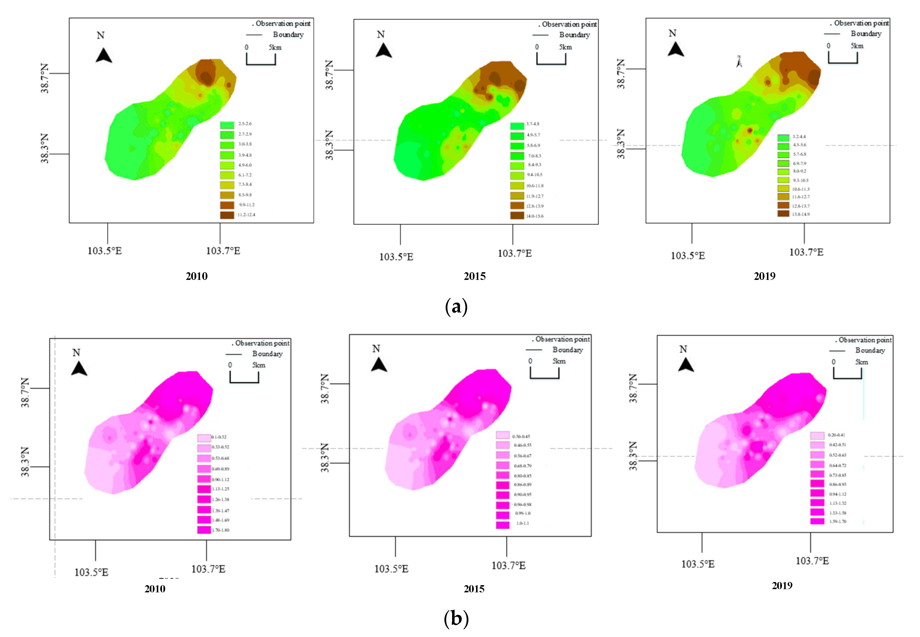
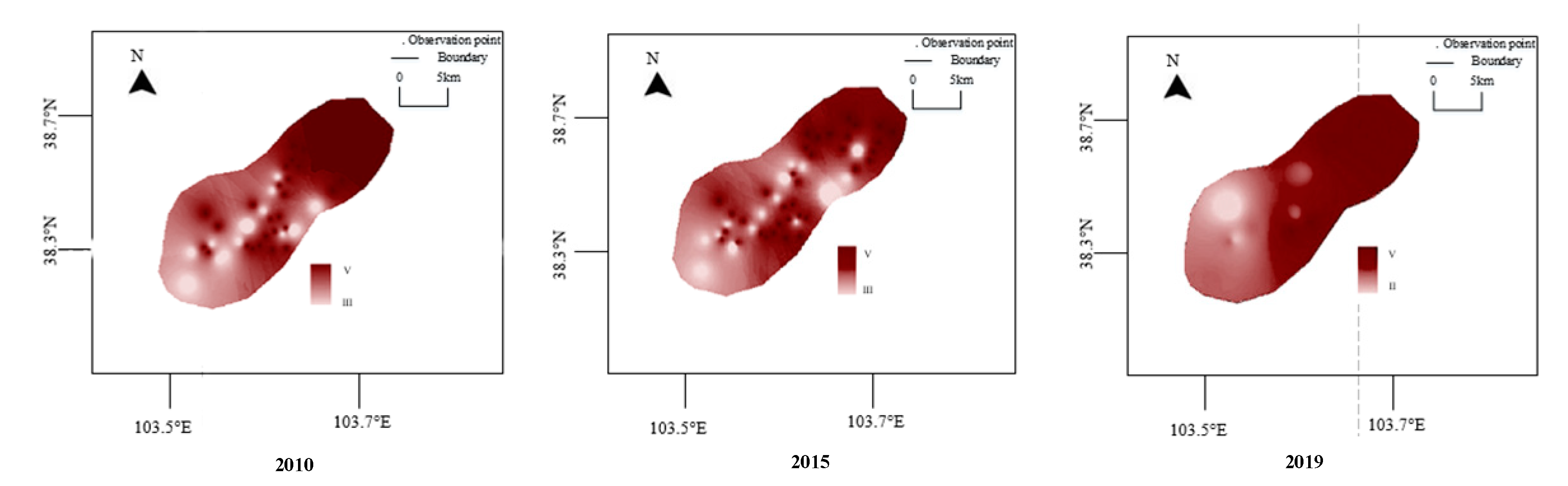
Taking permanganate and ammonia nitrogen as examples, the fitting results of the spatial distribution of the research area in three representative years are shown in Figure 4a,b below.
Based on above statistical results and fitting of spatial interpolation, the groundwater distribution characteristics in the research area could be known generally, so that the relevant characteristics of groundwater could be analyzed more deeply. For example, the overall spatial distribution of permanganate showed an increasing trend from 2010 to 2019, and the location closer to the north, the higher the content. It may be related to the trend of groundwater in the research area. The content of ammonia nitrogen increased from 2010 to 2015, while the content distribution decreased slightly from 2015 to 2019, showing the same spatial changes as permanganate; in addition, the content was higher in the observation wells near to the north.
3.3. Analysis on Predicated Result of Water Quality Based on the BPNN
Permanganate was taken as the benchmark, and the conventional BPNN and the GBPNN based on the gold section were applied to get the fitting process and predicted value in 2019, which is shown in Figure 5a,b.
The data changes in the figure reveal that the fitting result of permanganate of using the conventional NN is basically consistent with the distribution change trend of actual value, but the fitting result in a certain period is not ideal. In contrast, the GBPNN shows better overall prediction results, and its corresponding fitting and prediction accuracy have been improved to a certain extent.
Comparison results of the two algorithms on the predicted value and actual value of permanganate show that the conventional BPNN requires multiple debugging and iterations to reduce the variance to a lower level for the permanganate prediction. The average error corresponding to the conventional BPNN prediction results is about 12.88%, but the overall error distribution range is large, so the stability of water quality prediction has to be further strengthened. In contrast, the GBPNN has an average error of 6.49% among the six predictions. The prediction results in October and December are the best, and the error range of the entire prediction result is also at a lower level, so the overall prediction result is obviously better than the conventional BPNN. The reason is that GBPNN requires no repeated manual test on the network in determining the hidden layer of neurons, so it is more convenient to obtain the optimal solution and to predict water quality changes more accurate and comprehensive.
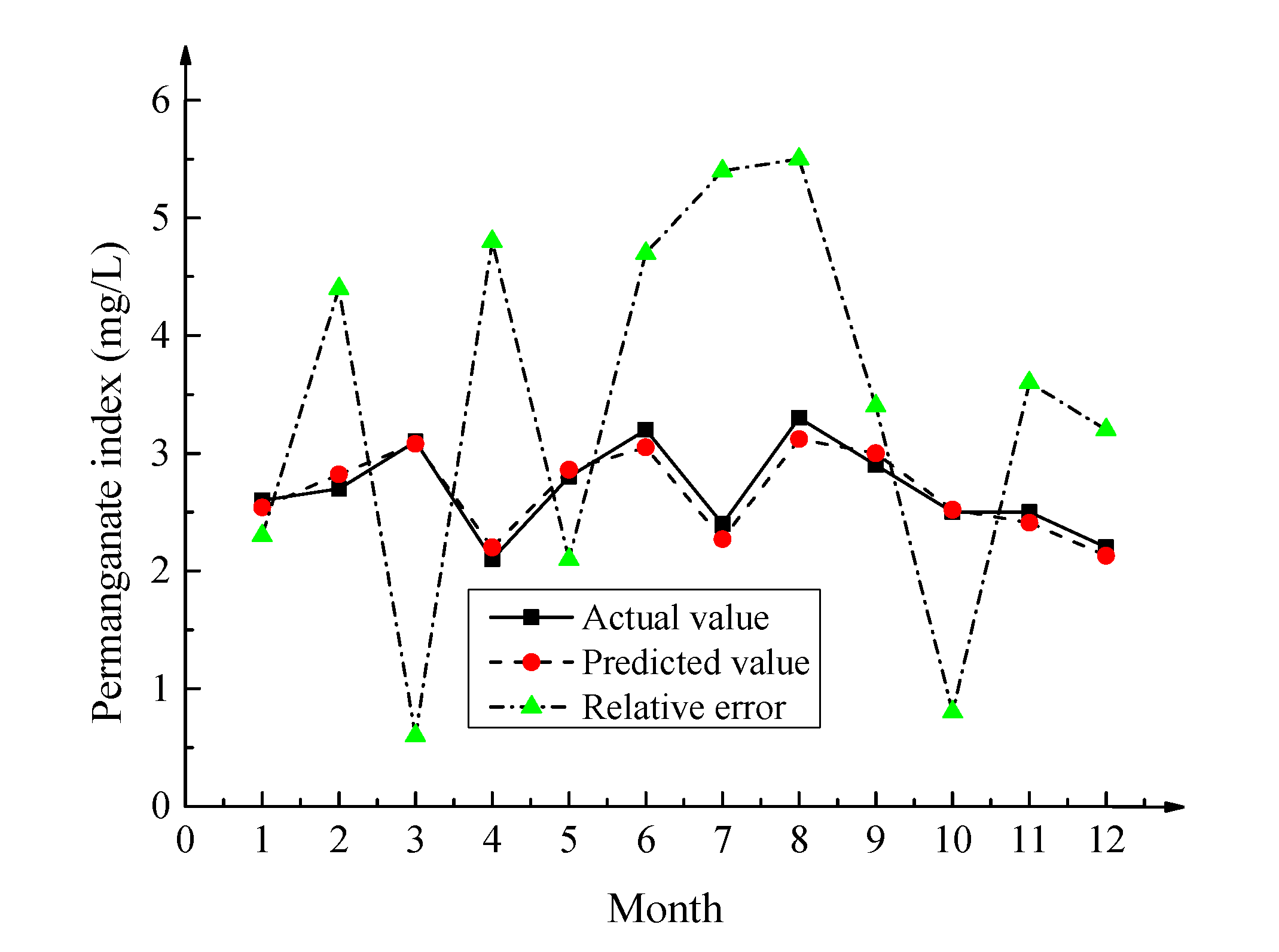
Permanganate was taken as the benchmark, and the WBPNNwas applied to obtain the prediction results for permanganate, as shown in Figure 6.
Figure 6 reveals that the application of the WBPNNhas greatly reduced the deviation between the predicted value and actual value of permanganate, but the overall trend of prediction on water quality is the same as the actual value. It indicates that the WBPNNis superior to the other two methods in the prediction results of water quality. The average error of the whole process is 3.66%, which is smaller than the previous two methods, and the distribution range of the error is relatively small. On the whole, the errors of the six predicted values are all below 10%. Therefore, the WBPNN has the best prediction effect.
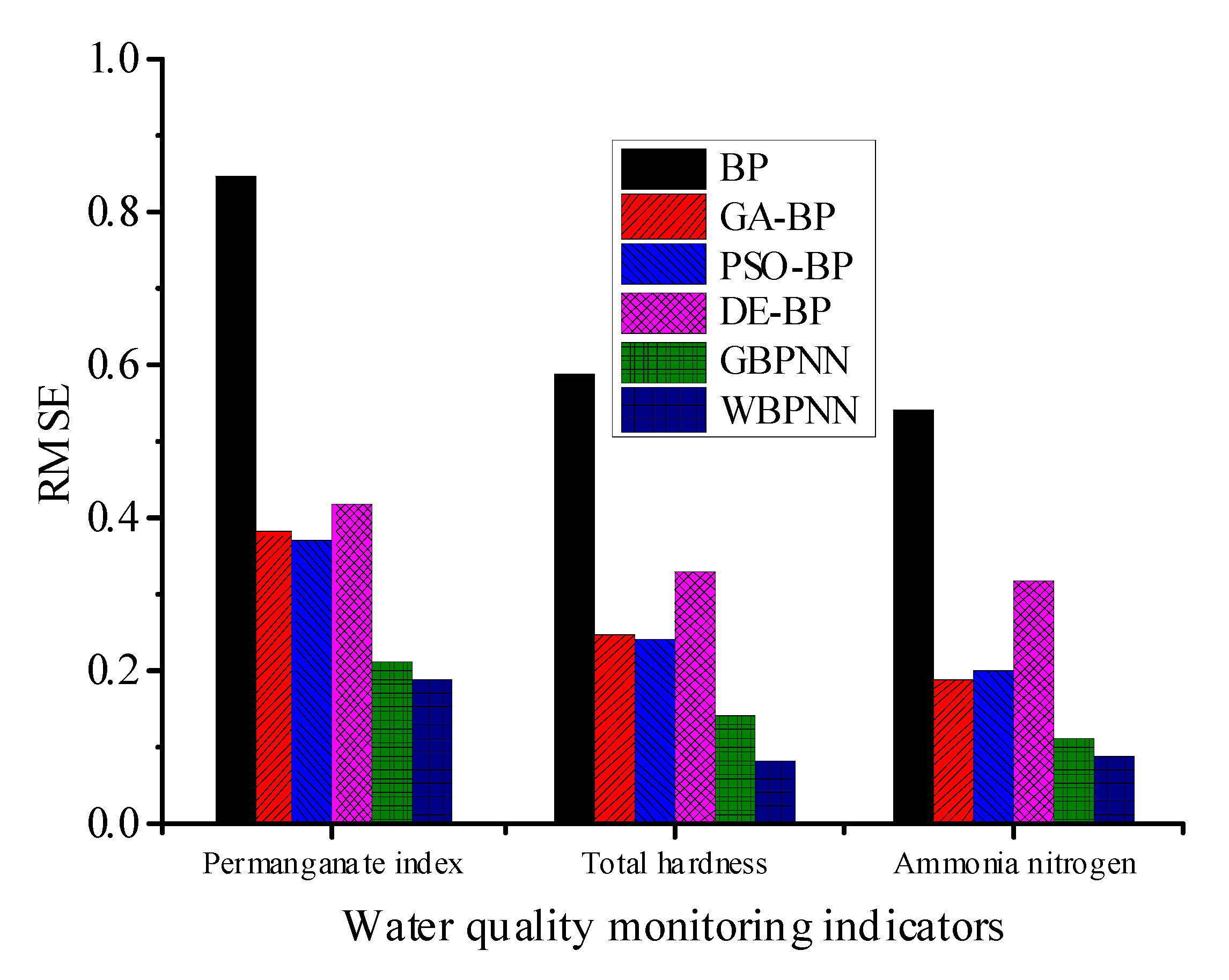
The RMSE of different algorithms based on permanganate, total hardness, and ammonia nitrogen are shown in Figure 7 below.
Figure 7 illustrates that the optimized BPNN has obviously lower error in predicting the key indicators of water quality in contrast to the conventional BPNN; the Genetical Analysis Back Propagation (GA-BP) is not obviously different from the Particle Swarm Optimization Back Propagation (PSO-BP), and Differential Evolutionary Back Propagation (DE-BP) is poorer than the above two algorithms; in addition, the GBPNN and WBPNN show lower RMSEs, and the WBPNN has the lowest RMSE and the best performance.
The prediction evaluation accuracies of different algorithms are shown in Figure 8 as follows.
Figure 8 reveals clearly that the WBPNN algorithm proposed in this study has better performance than other typical prediction algorithms in prediction evaluation accuracy of the water quality in the research area. The maximal prediction accuracy reaches 97.68%, the minimum value reaches 94.55%, so the average prediction accuracy is 96.12%. At this level, the prediction accuracy of the GBPNN algorithm is not significantly improved, which is similar to the DE-BP algorithm, and its performance is slightly inferior to the GA-BP algorithm and the PSO-BP algorithm. The above error statistical analysis results preliminarily prove the applicability and effectiveness of the WBPNN algorithm proposed in this study in water quality prediction.
3.4. Water Quality Level Prediction and Spatial Distribution Based on BPNN
Based on the above statistical analysis and comparison results, the WBPNN algorithm is applied to further verify its effectiveness. Based on the three representative years of 2010, 2015, and 2019 in the research area, the comprehensive prediction results of water quality in permanganate, total hardness, and ammonia nitrogen of six observation wells water quality grade are shown in Table 3 below.
The prediction evaluation results in the above table disclose that the prediction results obtained by using the WBPNN model can achieve basically consistent results except for a small number of differences in adjacent levels. Regarding the prediction results of the permanganate index, more than 80% of the prediction results in the three representative years are level IV; in the water quality prediction results of the total hardness, most of the prediction results in the three representative years are level V; and regarding the water quality prediction results of ammonia nitrogen, most of the prediction results in the three representative years are level III. It can be analyzed from this that from 2010 to 2015 and then to 2019, although the groundwater quality in the research area has been improved, the overall water quality is still poor. This may be related to human activities such as drilling wells and reclaiming wasteland. The decline of water level, the emergence of a series of problems such as soil salinization and intensified desertification, leads to the deterioration of water quality. Combining the statistical results of the key indicators of the three representative years in Table 1, it can be found that the use of the WBPNN model has shown excellent performance in the prediction of water quality.
Figure 9 shows the spatial distribution of groundwater quality level in the research area based on the GIS technology.
The prediction results and water quality spatial distribution prove that the proposed neural network models are effective in the groundwater quality prediction.
4. Discussion
The use of GIS technology can directly reflect the spatial distribution and changes of related things, which is of critical significance for the solution of many practical problems [24]. In the analysis of groundwater, water quality indexes can reveal relevant changes. The concentration changes of permanganate in 2014 and 2019 could reflect the status of organic pollution. Specifically, the higher the index value, the more serious the corresponding organic pollution.
In this study, the concentration of permanganate changes to varying degrees between 2014 and 2019, and the overall concentration of the research area is not high, indicating that the organic pollutants in the surface water and soil system of the research area can be effectively degraded and only a little is penetrated into the groundwater. The amount in the resource system is minimal. The concentration of TH in 2014 and 2019 is relatively high, which is a more obvious index of unqualified water in the research area. It is inseparable from the hydrogeographic characteristics of the research area [25]. In addition, the reason for higher TH concentration is that the rock contains more calcium and magnesium minerals, so that the initial content of the TH of the water layer is at a higher level. In short, the main reason for the higher concentration of TH lies in the lithology characteristics of the starting strata in the research area. Besides, another reason for the higher average concentration of TH is that a series of wastes generated by human activities in the research area infiltrate into the groundwater system through the soil, resulting in higher concentrations of calcium ions, magnesium ions, and other chemical components. The TH of groundwater reflects the degree of agricultural pollution from the side. The greater the TH, the more serious the agricultural pollution. This also reveals the deterioration of groundwater caused by agricultural pollution in the research area [26]. The N concentration is greatly affected by the natural environmental factors such as hydrogeology and precipitation in the research area. At the same time, it has a great relationship with human influence. However, the research area in this study is rich in agricultural resources, so the N content is relatively loose. The rocks have high mobility, which shows that agricultural production in this area has a great impact on the quality of groundwater. The distribution change of AN concentration at different monitoring points is closely related to the main types of production activities at each monitoring point, and the groundwater pollution in the research area in 2019 was more serious than in 2014 due to the sewage plants in the downstream. Therefore, it can realize an overall grasp and perception on the concentration distribution of the groundwater chemical characteristic indicators in the research area by selecting several representative indicators and applying GIS technology [27].
Taking permanganate as a benchmark, the BPNN and GBPNN are applied to the model for groundwater quality prediction for comparison, and the results prove that the WBPNNhas the best prediction result. The reason is that although the conventional BPNN model has some excellent characteristics in water quality prediction, the shortcomings such as slow convergence speed and difficulty in determining the number of hidden layer nodes in the application process cannot be ignored, which are clearly exposed in prediction of permanganate. The GBPNN based on the gold section effectively solves the shortcoming in determining the number of hidden layer nodes. Through the prediction results, it can also be found that whether the accuracy after optimized with the gold section in both data fitting and prediction result is improved to a certain degree. However, the GBPNN still fails to solve the problems of slow convergence and easy to fall into local optimal value. Then, the proposed WBPNNcombines the advantages of CWT and BPNN, and it can effectively solve the problems of slow convergence speed, poor search level, and easy to fall into local optimal value, so the final prediction results are more accurate. Therefore, the WBPNNis more applicable in the prediction of groundwater quality in Minqin County in this study. Analyzing the spatial distribution of groundwater quality based on the GIS technology and predicting the water quality in a targeted manner on this basis are of critical significance for further analyzing the distribution of groundwater resources in a certain area. Besser et al., (2017) analyzed the water chemistry of groundwater samples in southwestern Tunisia and found that natural component monitoring indicators had great impacts on groundwater quality, further confirming the prediction of groundwater quality based on natural component monitoring indicators in this study. The water quality can be determined based on the spatial distribution and prediction results of water chemical characteristics of groundwater. The comparative analysis with classical prediction algorithms proves the effectiveness of the proposed algorithm combined with GIS technology. It can have an overall perception of the spatial and temporal distribution characteristics and laws of groundwater in the research area. It indicates that the combination of neural network model and GIS technology is of great significance to improve the accuracy of groundwater quality prediction.
5. Conclusions
Through the statistics and analysis of the groundwater chemical characteristics in the research area, the spatial distribution of the water chemical key indicators in the research area was analyzed and discussed. Based on this, the BPNN model was introduced to predict and analyze the groundwater permanganate in the research area. The research results reveal the water chemical characteristics and spatial distribution rules of the research area, and theGBPNN has a great application potential in the prediction of groundwater quality. In contrast to several classic algorithms, the proposed WBPNN shows superior performance, and it can explore the spatial distribution rules of groundwater more deeply by combining with the GIS technology. However, there are still some shortcomings in the study. Due to the influence of multiple factors, the indicators selected in the spatial distribution analysis of the groundwater chemical characteristics of the research area are not comprehensive enough. Besides, the groundwater quality level is not evaluated one by one. Therefore, it is necessary to conduct a deep study in the future.
Author Contributions
Conceptualization, formal analysis, writing-Original Draft Preparation: Jing Sun; Writing-Review & Editing, supervision: Genhou Wang. All authors have read and agreed to the published version of the manuscript.
Funding
This research was funded by General Project of the National Natural Science Foundation of China, grant number 41372249.
Conflicts of Interest
The authors declare no conflict of interest.
References
- Jiang, Q.; Wang, T.; Wang, Z.; Fu, Q.; Zhou, Z.; Zhao, Y.; Dong, Y. HHM- and RFRM-Based Water Resource System Risk Identification. Water Resour. Manag. 2018, 32, 4045–4061. [Google Scholar] [CrossRef]
- Kumar, P.; Johnson, B.A.; Dasgupta, R.; Avtar, R.; Chakraborty, S.; Kawai, M.; Magcale-Macandog, D.B. Participatory Approach for More Robust Water Resource Management: Case Study of the Santa Rosa Sub-Watershed of the Philippines. Water 2020, 12, 1172. [Google Scholar] [CrossRef] [Green Version]
- Nistor, M.-M. Climate change effect on groundwater resources in South East Europe during 21st century. Quat. Int. 2019, 504, 171–180. [Google Scholar] [CrossRef]
- Borji, M.; Nia, A.M.; Malekian, A.; Salajegheh, A.; Khalighi, S. Comprehensive evaluation of groundwater resources based on DPSIR conceptual framework. Arab. J. Geosci. 2018, 11, 158. [Google Scholar] [CrossRef]
- Xiao, K.; Li, H.; Shananan, M.; Zhang, X.; Wang, X.; Zhang, Y.; Zhang, X.; Liu, H. Coastal water quality assessment and groundwater transport in a subtropical mangrove swamp in Daya Bay, China. Sci. Total. Environ. 2019, 646, 1419–1432. [Google Scholar] [CrossRef]
- Mohana, P.; Velmurugan, P.M. Geochemical Characterization and Water Quality Assessment of Groundwater in Arani Taluk of Tamil Nadu, South India. Geochem. Int. 2020, 58, 598–612. [Google Scholar] [CrossRef]
- Ostad-Ali-Askari, K.; Shayannejad, M.; Ghorbanizadeh-Kharazi, H. Artificial neural network for modeling nitrate pollution of groundwater in marginal area of Zayandeh-rood River, Isfahan, Iran. KSCE J. Civ. Eng. 2017, 21, 134–140. [Google Scholar] [CrossRef]
- Zanotti, C.; Rotiroti, M.; Fumagalli, L.; Stefania, G.; Canonaco, F.; Stefenelli, G.; Prévôt, A.; Leoni, B.; Bonomi, T. Groundwater and surface water quality characterization through positive matrix factorization combined with GIS approach. Water Res. 2019, 159, 122–134. [Google Scholar] [CrossRef]
- Johnny, J.C.; Sashikkumar, M.C.; Kirubakaran, M.; Mathi, L.M. GIS-based assessment of groundwater quality and its suitability for drinking and irrigation purpose in a hard rock terrain: A case study in the upper Kodaganar basin, Dindigul district, Tamil Nadu, India. Desalin. Water Treat 2018, 102, 49–60. [Google Scholar] [CrossRef]
- Lee, S.; Lee, S.; Lee, M.-J.; Jung, H.-S. Spatial Assessment of Urban Flood Susceptibility Using Data Mining and Geographic Information System (GIS) Tools. Sustainability 2018, 10, 648. [Google Scholar] [CrossRef] [Green Version]
- Daful, M.; Ezeamaka, C.; Ogbole, M.; Sani, H.; Sadiq, Q. The Application of Remote Sensing and Geographic Information System in Assessing Probable Tsetse Flies Habitats in Ikom LGA, Cross River State, Nigeria. Environ. Earth Sci. Res. J. 2019, 6, 19–23. [Google Scholar] [CrossRef]
- Lozano-Jaramillo, M.; Bastiaansen, J.W.M.; Dessie, T.; Komen, H. Use of geographic information system tools to predict animal breed suitability for different agro-ecological zones. Animals 2019, 13, 1536–1543. [Google Scholar] [CrossRef] [PubMed] [Green Version]
- Jiang, Y.; Zhou, L.; Tucker, C.J.; Raghavendra, A.; Hua, W.; Liu, Y.Y.; Joiner, J. Widespread increase of boreal summer dry season length over the Congo rainforest. Nat. Clim. Chang. 2019, 9, 617–622. [Google Scholar] [CrossRef]
- Sun, M.; Ren, A.-X.; Lim, S.Y.; Wang, P.-R.; Mo, F.; Xue, L.-Z.; Lei, M.-M. Long-term evaluation of tillage methods in fallow season for soil water storage, wheat yield and water use efficiency in semiarid southeast of the Loess Plateau. Field Crop. Res. 2018, 218, 24–32. [Google Scholar] [CrossRef]
- Dong, G.; Huang, W.; Smith, W.A.P.; Ren, P. Filling Voids in Elevation Models Using a Shadow-Constrained Convolutional Neural Network. IEEE Geosci. Remote. Sens. Lett. 2020, 17, 592–596. [Google Scholar] [CrossRef]
- Ertin, D.G.; Karakaya, A.B.; Ozyavuz, M. Edirne Saraclar street pedestrian comfort analysis. J. Environ. Prot. Ecol. 2018, 19, 738–751. [Google Scholar]
- Al-Waeli, A.H.; Sopian, K.; Kazem, H.A.; Yousif, J.H.; Chaichan, M.T.; Ibrahim, A.; Mat, S.; Ruslan, M.H. Comparison of prediction methods of PV/T nanofluid and nano-PCM system using a measured dataset and artificial neural network. Sol. Energy 2018, 162, 378–396. [Google Scholar] [CrossRef]
- He, F.; Zhang, L. Prediction model of end-point phosphorus content in BOF steelmaking process based on PCA and BPNN. J. Process Contr. 2018, 66, 51–58. [Google Scholar] [CrossRef]
- Liu, C.; Zhao, Z.; Wen, G. Adaptive neural network control with optimal number of hidden nodes for trajectory tracking of robot manipulators. Neurocomputing 2019, 350, 136–145. [Google Scholar] [CrossRef]
- Li, D.; Cheng, T.; Jia, M.; Zhou, K.; Lu, N.; Yao, X.; Tian, Y.; Zhu, Y.; Cao, W. PROCWT: Coupling PROSPECT with continuous wavelet transform to improve the retrieval of foliar chemistry from leaf bidirectional reflectance spectra. Remote. Sens. Environ. 2018, 206, 14. [Google Scholar] [CrossRef] [Green Version]
- Ince, H.; Cebeci, A.F.; Imamoglu, S.Z. An Artificial Neural Network-Based Approach to the Monetary Model of Exchange Rate. Comput. Econ. 2017, 53, 817–831. [Google Scholar] [CrossRef]
- Gao, Y.; Zhou, X.; Ren, J.; Zhao, Z.; Xue, F. Electricity Purchase Optimization Decision Based on Data Mining and Bayesian Game. Energies 2018, 11, 1063. [Google Scholar] [CrossRef] [Green Version]
- Zuxing, C.; Dian, W. A Prediction Model of Forest Preliminary Precision Fertilization Based on Improved GRA-PSO-BP Neural Network. Math. Probl. Eng. 2020, 2020, 17. [Google Scholar] [CrossRef]
- Lee, M.; Hong, T. Hybrid agent-based modeling of rooftop solar photovoltaic adoption by integrating the geographic information system and data mining technique. Energy Convers. Manag. 2019, 183, 266–279. [Google Scholar] [CrossRef]
- Besser, H.; Mokadem, N.; Redhouania, B.; Rhimi, N.; Khlifi, F.; Ayadi, Y.; Omar, Z.; Bouajila, A.; Hamed, Y. GIS-based evaluation of groundwater quality and estimation of soil salinization and land degradation risks in an arid Mediterranean site (SW Tunisia). Arab. J. Geosci. 2017, 10, 350. [Google Scholar] [CrossRef]
- Chen, C.; Cheng, T.; Zhang, X.; Wu, R.; Wang, Q. Synthesis of an efficient Pb adsorption nano-crystal under strong alkali hydrothermal environment using a gemini surfactant as directing agent. J. Chem. Soc. Pak. 2019, 41, 1034–1038. [Google Scholar]
- Yan, X.; Chen, M.; Chen, M.-Y. Coupling and Coordination Development of Australian Energy, Economy, and Ecological Environment Systems from 2007 to 2016. Sustainability 2019, 11, 6568. [Google Scholar] [CrossRef] [Green Version]
Figure 1.
Geographical location of the study area.
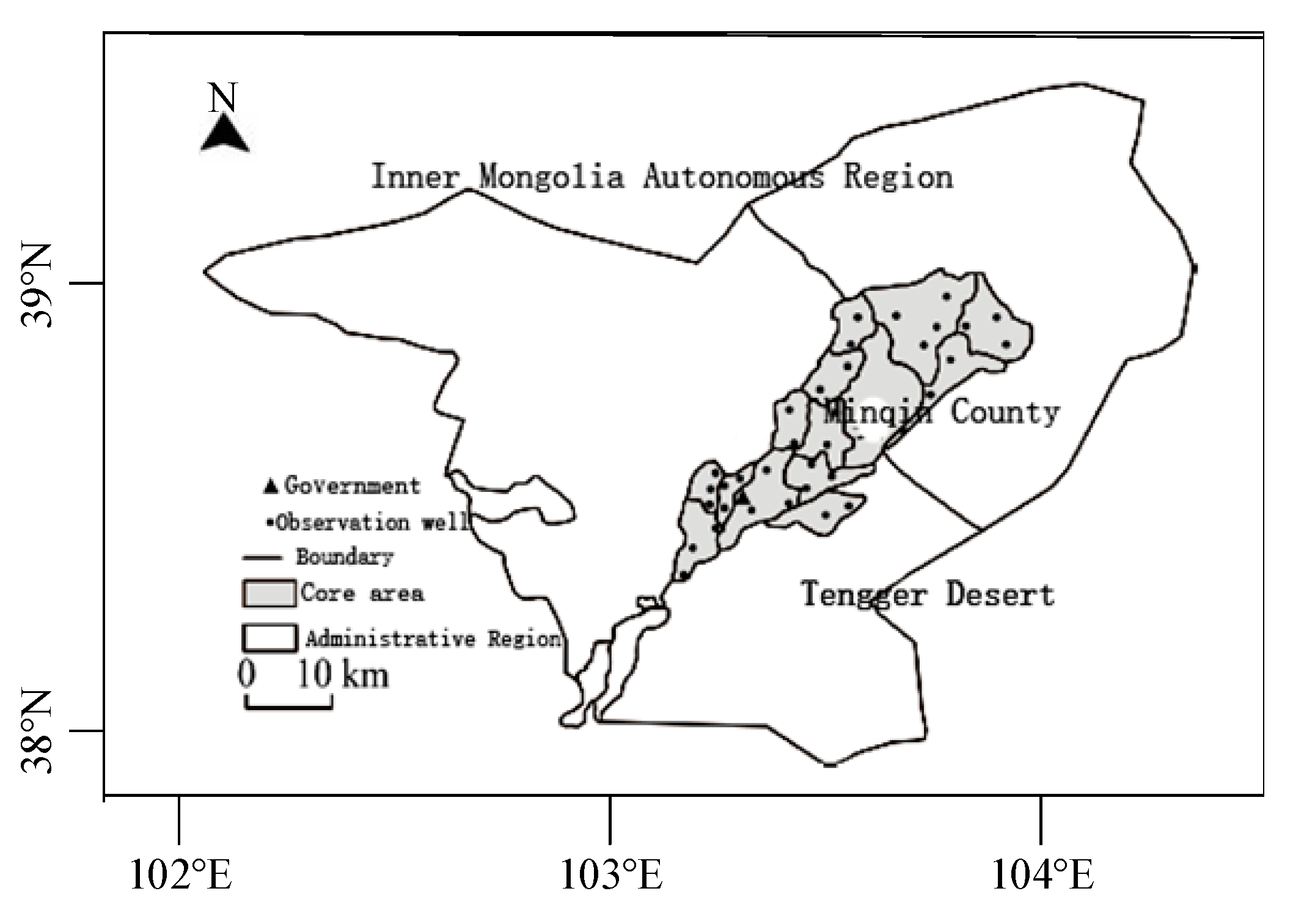
Figure 2.
The distribution of spatial interpolation sites in the selected research area under different representative years.
Figure 2.
The distribution of spatial interpolation sites in the selected research area under different representative years.
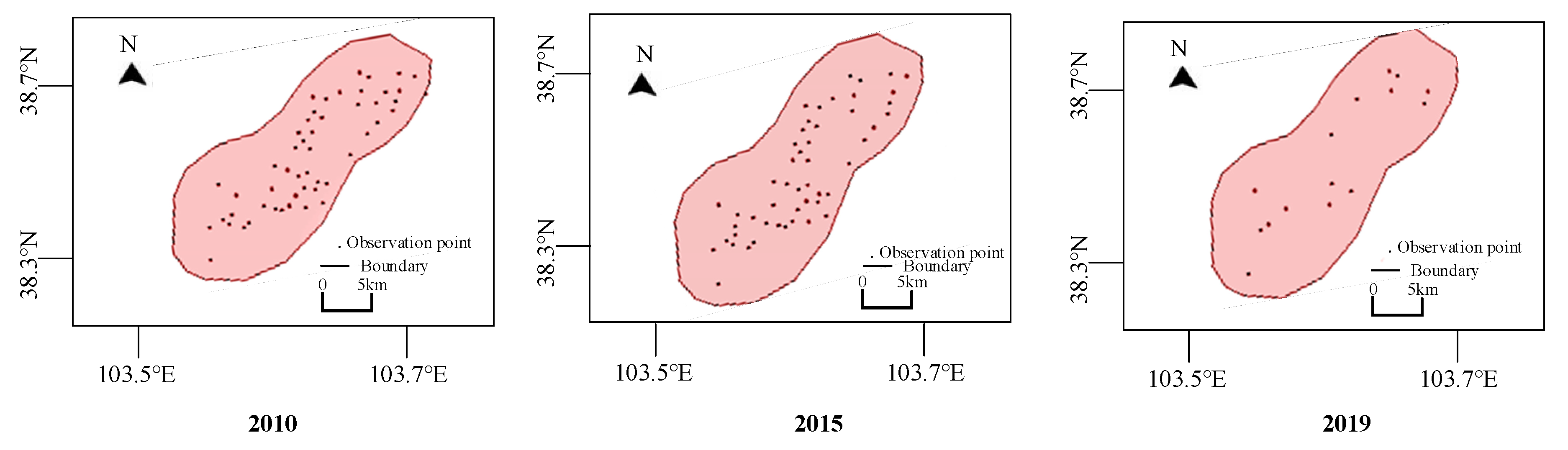
Figure 3.
Distribution and changes on concentrations of monitored indicators. (In the above figures, P, AS, AN, TH, TS, S, Cl, Na, N-1, and F refers to the permanganate, anionic surfactant, ammonia nitrogen, total hardness, total dissolved solids, sulfate, nitrate, chloride, sodium, nitrite, and fluoride, respectively.) Note: considering that there are multiple monitoring indexes, the results are given in two figures.
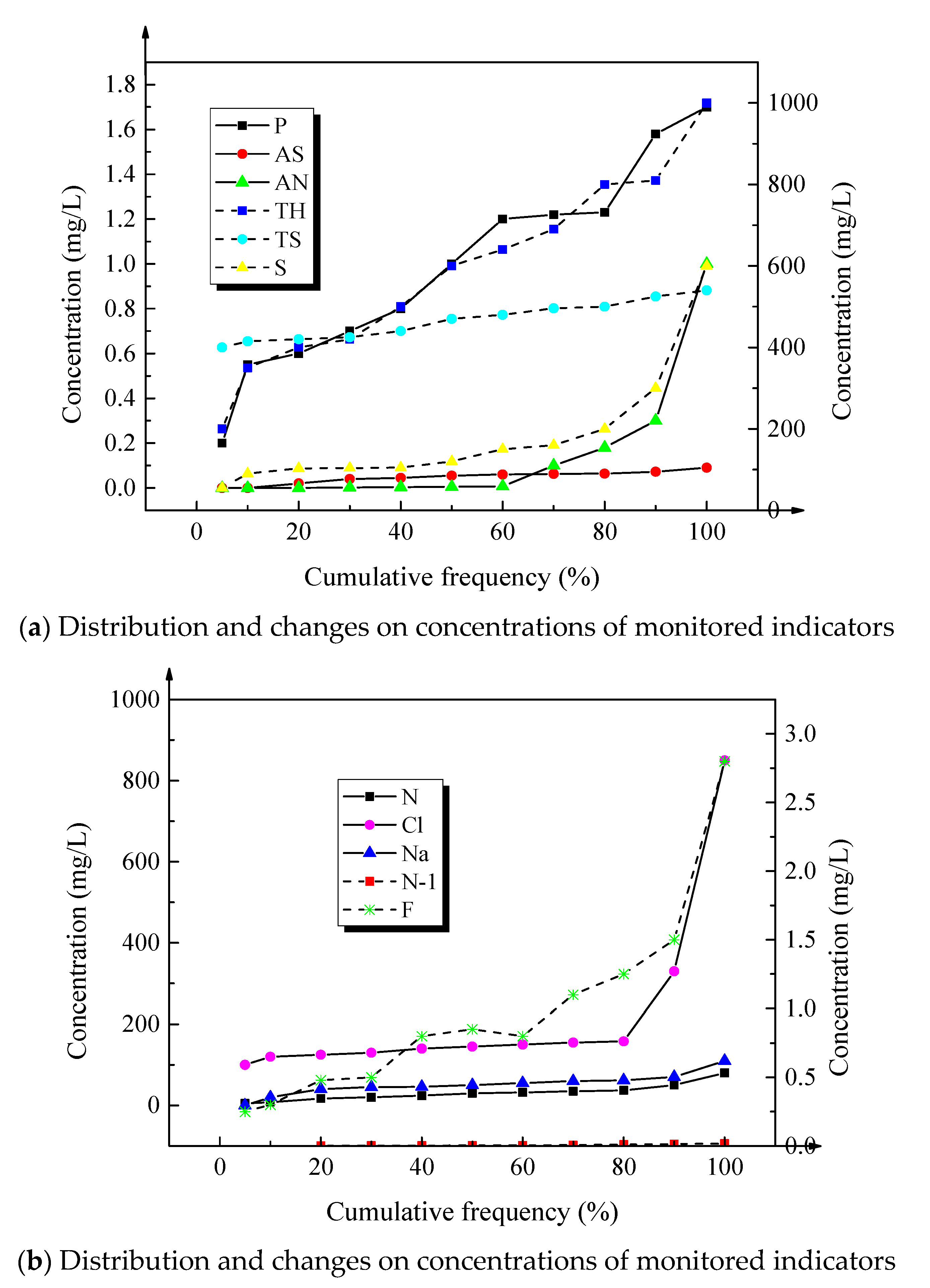
Figure 4.
Fitting results of the spatial distribution of the research area: (a) shows the results based on permanganate, and (b) shows the results based on ammonia nitrogen.
Figure 4.
Fitting results of the spatial distribution of the research area: (a) shows the results based on permanganate, and (b) shows the results based on ammonia nitrogen.

Figure 5.
Comparison on data fitting and predicated value of conventional back propagation (BP) neural network (BPNN) and golden section (GBPNN) to permanganate. (a) data fitting; (b) prediction results.
Figure 5.
Comparison on data fitting and predicated value of conventional back propagation (BP) neural network (BPNN) and golden section (GBPNN) to permanganate. (a) data fitting; (b) prediction results.
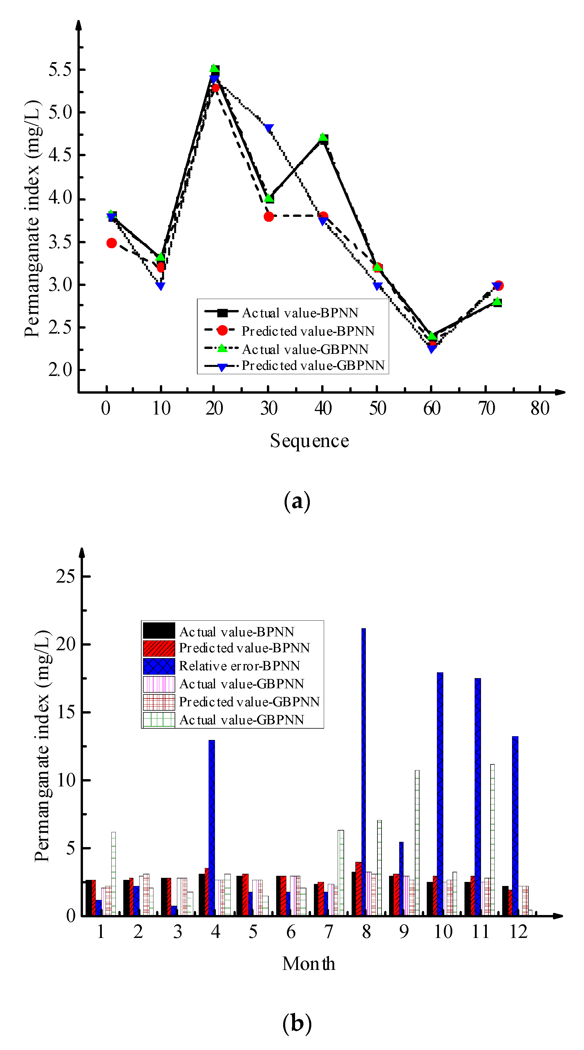
Figure 6.
The prediction results of wavelet transform (WBPNN)for permanganate.

Figure 7.
Statistic results of water prediction based on the RMSE.

Figure 8.
Statistical results of water prediction based on the prediction evaluation accuracy.
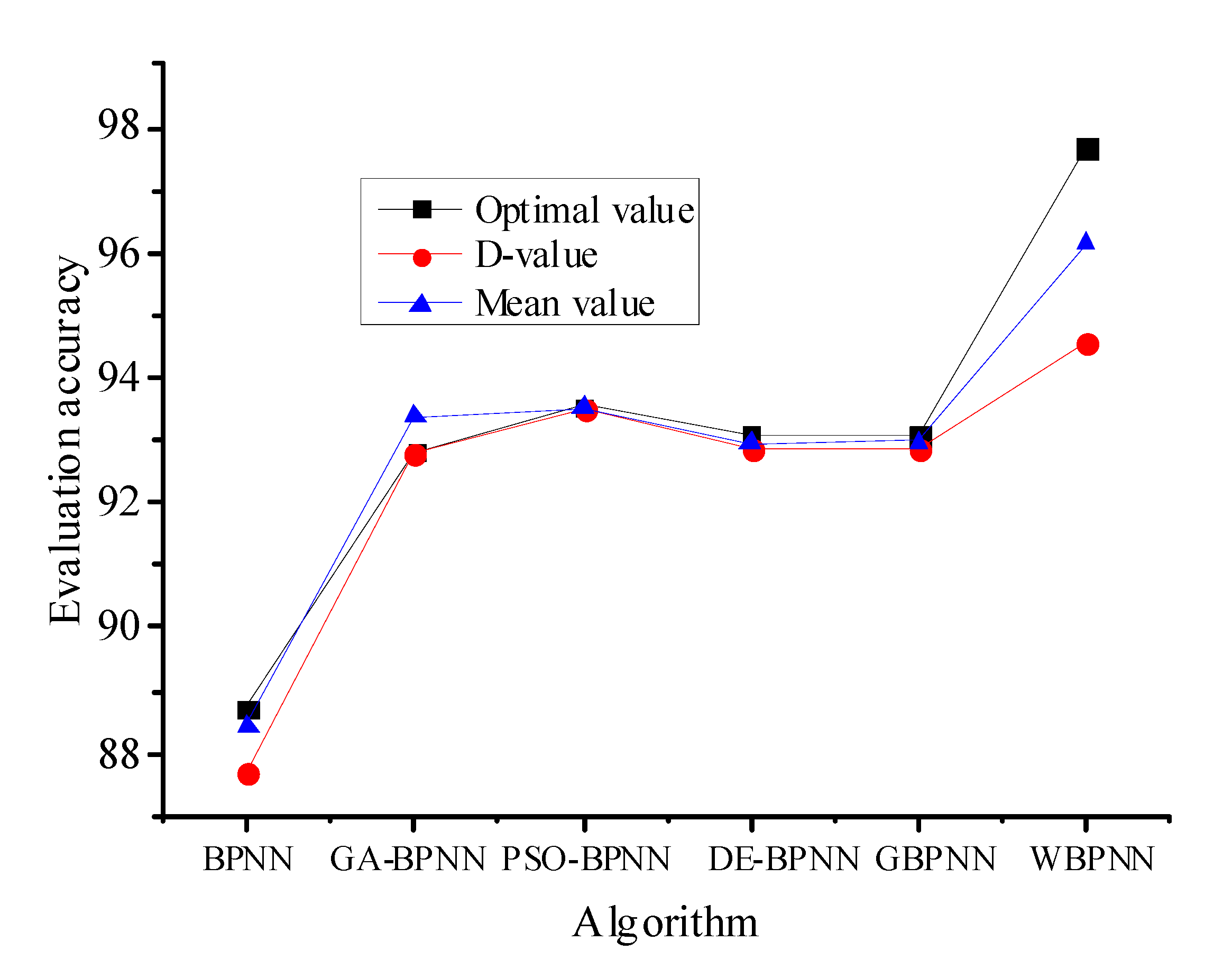
Figure 9.
Spatial distribution of groundwater quality in the research area of the three representative years.
Figure 9.
Spatial distribution of groundwater quality in the research area of the three representative years.


Table 1.
Statistical results for water chemical elements of groundwater in selected representative years.
Table 1.
Statistical results for water chemical elements of groundwater in selected representative years.
| Chemical Element | Maximal | Minimal | Mean | Standard Deviation | Variable Coefficient |
|---|---|---|---|---|---|
| Permanganate | 12.4 (2010) | 2.5 (2010) | 7.5 (2010) | 2.94 (2010) | 1.44 (2010) |
| 15.6 (2015) | 3.7 (2010) | 9.7 (2015) | 1.88 (2015) | 1.51 (2015) | |
| 14.9 (2019) | 3.2 (2019) | 9.1(2019) | 1.55 (2019) | 0.99 (2019) | |
| Ammonia nitrogen | 1.8 (2010) | 0.1 (2010) | 0.9 (2010) | 2.38 (2010) | 1.72 (2010) |
| 1.1 (2015) | 0.3 (2015) | 0.7 (2015) | 2.72 (2015) | 0.99 (2015) | |
| 1.7 (2019) | 0.2 (2019) | 0.9 (2019) | 2.59 (2019) | 1.22 (2019) | |
| SO42- | 3146.2 (2010) | 205.6 (2010) | 979.5 (2010) | 796.3 (2010) | 0.82 (2010) |
| 2253.1(2015) | 85.6 (2015) | 907.9 (2015) | 700.6 (2015) | 0.78 (2015) | |
| 2118.2 (2019) | 102.9 (2019) | 792.2 (2019) | 674.4 (2019) | 0.86 (2019) | |
| Total hardness | 5126.4 (2010) | 227.9 (2010) | 1082.4 (2010) | 70.2 (2010) | 1.16 (2010) |
| 1973.2 (2015) | 152.2 (2015) | 922.2 (2015) | 605.5 (2015) | 1.37 (2015) | |
| 2087.1 (2019) | 156.2 (2019) | 779.9 (2019) | 583.6 (2019) | 0.76 (2019) | |
| Ca2+ | 304.5 (2010) | 36.8 (2010) | 144.6 (2010) | 90.5 (2010) | 0.64 (2010) |
| 279.7 (2015) | 29.8 (2015) | 144.3 (2015) | 80.9 (2015) | 0.57 (2015) | |
| 346.8 (2019) | 6.5 (2019) | 115.6 (2019) | 85.7 (2019) | 0.75 (2019) | |
| Mg2+ | 495.8 (2010) | 32.6 (2010) | 135.4 (2010) | 125.5 (2010) | 0.94 (2010) |
| 330.6 (2015) | 19.1 (2015) | 136.5 (2015) | 107.3 (2015) | 0.78 (2015) | |
| 336.9 (2019) | 7.5 (2019) | 108.4 (2019) | 109.6 (2019) | 1.02 (2019) | |
| Na+ and K+ | 953.7 (2010) | 54.8 (2010) | 394.3 (2010) | 275.2 (2020) | 0.71 (2010) |
| 856.6 (2015) | 44.5 (2015) | 383.8 (2015) | 290.5 (2015) | 0.77 (2015) | |
| 918.2 (2019) | 20.7 (2019) | 356.9 (2019) | 326.8 (2019) | 0.93 (2019) | |
| Nitrate | 1.7 (2010) | 0.01 (2010) | 0.13 (2010) | 0.5 (2010) | 0.75 (2010) |
| 78.2 (2015) | 0.6 (2015) | 19.58 (2015) | 24.1 (2015) | 0.24 (2015) | |
| 95.9 (2019) | 0.0 (2019) | 0.03 (2019) | 0.3 (2019) | 0.62 (2019) |
Note: variable coefficient refers to the ratio between the standard deviation and mean; the unit for maximal, minimal, and mean is mg/L.
Table 2.
Water quality level and content of permanganate, total hardness, and ammonia nitrogen.
| Indicator | I. | II. | III. | IV. | V. |
|---|---|---|---|---|---|
| Permanganate | 0–2.0 | 2.0–4.0 | 4.0–6.0 | 6.0–10.0 | 10.0–15.0 |
| Total hardness | 0–150 | 150–300 | 300–450 | 450–550 | >550 |
| Ammonia nitrogen | 0–0.15 | 0.15–0.50 | 0.50–1.0 | 1.0–1.5 | 1.5–2.0 |
Note: the unit for permanganate, total hardness, and ammonia nitrogen is mg/L.
Table 3.
Prediction results of water quality level based on the WBPNN.
| Observation Well | Predicted Water Quality Level | ||||||||
|---|---|---|---|---|---|---|---|---|---|
| 2010 | 2015 | 2019 | |||||||
| PI | TH | AN | PI | TH | AN | PI | TH | AN | |
| 176 | IV | V | III | V | IV | III | IV | V | III |
| 167 | IV | V | III | IV | V | III | IV | V | III |
| 159 | IV | V | III | IV | V | IV | III | V | II |
| 142 | V | V | IV | IV | V | III | IV | V | III |
| 132 | IV | IV | IV | V | III | III | IV | IV | IV |
| 112 | V | V | III | IV | V | III | IV | V | III |
Note: PI, TH, and AN refer to permanganate, total hardness, and ammonia nitrogen, respectively.
Publisher’s Note: MDPI stays neutral with regard to jurisdictional claims in published maps and institutional affiliations. |
© 2020 by the authors. Licensee MDPI, Basel, Switzerland. This article is an open access article distributed under the terms and conditions of the Creative Commons Attribution (CC BY) license (http://creativecommons.org/licenses/by/4.0/).
Share and Cite
MDPI and ACS Style
Sun, J.; Wang, G. Geographic Information System Technology Combined with Back Propagation Neural Network in Groundwater Quality Monitoring. ISPRS Int. J. Geo-Inf. 2020, 9, 736. https://doi.org/10.3390/ijgi9120736
AMA Style
Sun J, Wang G. Geographic Information System Technology Combined with Back Propagation Neural Network in Groundwater Quality Monitoring. ISPRS International Journal of Geo-Information. 2020; 9(12):736. https://doi.org/10.3390/ijgi9120736
Chicago/Turabian StyleSun, Jing, and Genhou Wang. 2020. "Geographic Information System Technology Combined with Back Propagation Neural Network in Groundwater Quality Monitoring" ISPRS International Journal of Geo-Information 9, no. 12: 736. https://doi.org/10.3390/ijgi9120736
Note that from the first issue of 2016, this journal uses article numbers instead of page numbers. See further details here.