Multifaceted Geometric Assessment towards Simplified Urban Surfaces Built by 3D Reconstruction


1
College of Space Information, Space Engineering University, Beijing 101416, China
2
State Key Laboratory of High Performance Computing, College of Computer, National University of Defense Technology, Changsha 410073, China
*
Authors to whom correspondence should be addressed.
ISPRS Int. J. Geo-Inf. 2019, 8(8), 360; https://doi.org/10.3390/ijgi8080360
Submission received: 14 May 2019
/
Revised: 31 July 2019
/
Accepted: 7 August 2019
/
Published: 14 August 2019
Abstract
:Large-scale three-dimensional (3D) reconstruction from multi-view images is used to generate 3D mesh surfaces, which are usually built for urban areas and are widely applied in many research hotspots, such as smart cities. Their simplification is a significant step for 3D roaming, pattern recognition, and other research fields. The simplification quality has been assessed in several studies. On the one hand, almost all studies on surface simplification have measured simplification errors using the surface comparison tool Metro, which does not preserve sufficient detail. On the other hand, the reconstruction precision of urban surfaces varies as a result of homogeneity or heterogeneity. Therefore, it is difficult to assess simplification quality without surface classification. These difficulties are addressed in this study by first classifying urban surfaces into planar surfaces, detailed surfaces, and urban frameworks according to the simplification errors of different types of surfaces and then measuring these errors after sampling. A series of assessment indexes are also provided to contribute to the advancement of simplification algorithms.
1. Introduction
Mesh surfaces are used universally in computer graphics [1], virtual reality [2], and computer aided design (CAD) [3]. A triangular mesh—in other words, an irregular triangular network (TIN)—is practical because of its simplicity and stable geometry. Traditionally, surfaces have been simplified or subdivided to meet the requirements of high precision for mainframes and low precision for mobile terminals. Simplification is frequently applied in the domains of 3D reconstruction because of the large data volume. Problems such as high power consumption and high cost are among the drawbacks of other 3D modeling methods, such as the use of the bands of infrared spectra [4] or visible light, namely, Light Detection and Ranging (LiDAR) [5]. Moreover, such methods lack transparency, so they are easily detected and intercepted in military operations. The TIN in this study is generated by stereo images photographed by oblique cameras that are on board of airplanes. Oblique photogrammetry can be achieved by many methods, such as Structure-from-Motion (SfM) [6]. Of all the types of surfaces, urban surfaces, which is the topic of this article, are widely used in marketing, disaster relief, and urban planning, among other applications [7].
Surface simplification is of great significance in processing the products generated by 3D reconstruction from stereo aerial photographs. First, it simplifies the large amount of data that result from some methods. For example, the patch-based multi-view stereo algorithm [8] requires at least 32 GB memory from 50 aerial photographs with a resolution of for 3D reconstruction. Such data volume wastes storage facilities or bandwidth, and it places immense pressure on the graphics processing unit (GPU). Second, simplified surfaces are applied in the domains of pattern recognition. The details of simplified urban surfaces are unique traits in pattern recognition, such as saliency detection in Ref. [9]. Therefore, the preservation of traits in simplified surfaces is crucial.
The traits of urban surfaces are detailed, except for planar objects, such as roads and the sides of buildings. Among characteristics of planar surfaces, urban frameworks, which are the sides of planar surfaces such as building borders, are crucial for the semantic recognition of urban surfaces in 3D reconstruction methods, such as plane-based regularization in Ref. [10]. Both of the above-mentioned emphases of urban surfaces are heterogeneous, and their extraction and assessment for purposes such as error measurement are of enormous significance. On the one hand, homogeneous portions such as planar surfaces (eliminated through the extraction of detailed surfaces) and vegetation (eliminated through extraction of urban frameworks) are difficult to reconstruct accurately. For example, a specific study was done to discern the texture of asphalt pavement using a popular method, namely, SIFT (Scale Invariant Feature Transform) [11], and it highlighted the difficulty of distinguishing between objects with similar textures. Therefore, research efforts on the simplification of urban surfaces tend to regard such surfaces above as absolutely planar [10] and focus on the precision of heterogeneous details instead [12,13]. Vegetation is a component of detailed surfaces, potentially making the assessment results lack heterogeneity, which emphasizes the necessity of extracting and evaluating urban frameworks. On the other hand, detailed surfaces and urban frameworks are easily recognized if distortion occurs. Additionally, urban frameworks are applied in many areas, such as archeology [14] and urban planning [15]. They are entirely heterogeneous, so they have high precision. Even corners and edges with similar or the same texture have a homogeneous appearance as a result of different ambient light rejection characteristics, which are easily grasped by SIFT [11], plane-based regularization [10], and other reconstruction methods using stereo images. In sum, detailed surfaces and urban frameworks are key and need to be preserved after simplification, and they contribute to the assessments performed after they are extracted.
Given the above-discussed phenomena of surface simplification, this article focuses on the assessment of urban surfaces after simplification, which is a necessary process after extraction. This article, which reports a method that was developed and performed for the numerical assessment of simplified urban surfaces, is presented as follows. In Section 2, related works are briefly reviewed. Section 3 presents the approach developed in this study for dividing urban surfaces. Section 4 illustrates the sampling techniques used for distance calculations for the measurement of errors. Section 5 describes numerical indexes that are based on surface classification and used in the surface assessment procedure. Section 6 details the experiments performed to assess the quality of simplification algorithms. The aim of these experiments is to further improve the algorithms introduced in Section 2 and to choose the optimal variable parameters for the improved algorithm.
2. Related Work
2.1. Current Surface Assessment Methods
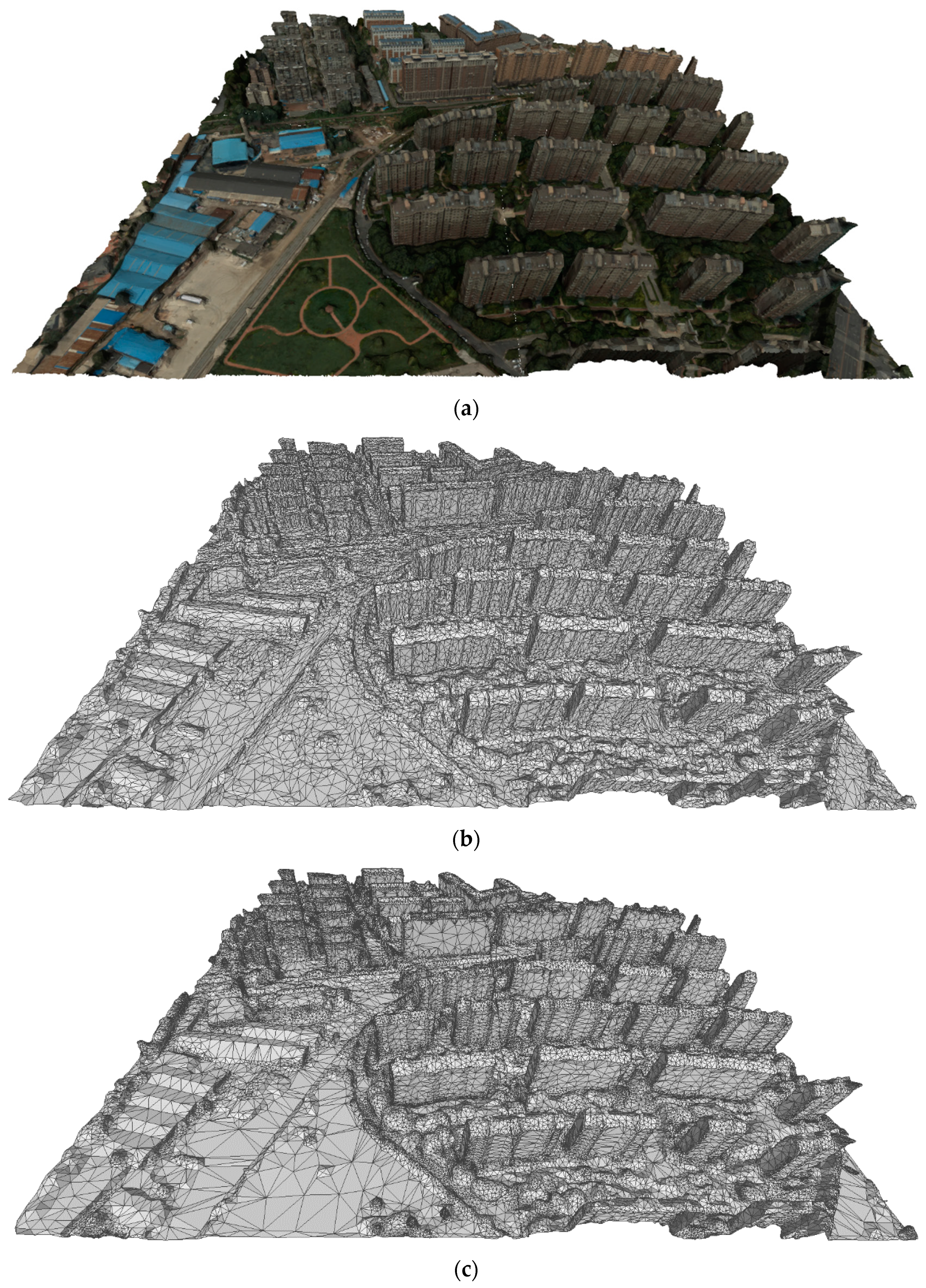
The 3D reconstruction of surfaces is performed using a large-scale reconstruction algorithm—namely, multi-photo geometrically constrained least-squares matching (MPGC) [16], which is already embedded in the MVE software [17]—with the aid of cluster segmentation based on luminosity similarity [18]. Therefore, a scene consists of numerous tiles. After hole-filling [19], surface tessellation is completed. The resulting tiles are the basic material studied in this research.
The assessment of simplified surfaces can be roughly classified into three categories:
- Almost all the research in the literature on surface simplification has focused on describing the effects after limited exhibition of simplified results. However, this approach is too subjective. As illustrated in Figure 1, even without consideration of the uneven precision of 3D reconstruction, the interpretation of results using traditional methods often faces this challenge.
- Another type of assessment is the measurement of comprehensive error, including Hausdorff error, mean error, and RMS error, using a tool called Metro [20], which is lacking in the demonstration of the error of important details, as shown in Figure 2. The series of indexes applied in our work aims to solve this weakness.
- The third method relies on indexes that are related to the simplification algorithms, which can be prone to circular arguments. They also lack robustness, so it is extremely difficult to compare them with other algorithms according to these quantified indexes.
Even the recent studies on surface simplification have performed assessments that mainly rely on Metro. There have been many evaluations of surface simplification [21,22,23,24,25,26,27,28] that measure comprehensive errors, but the results of different studies are contradictory. Some reports on surface simplification have regarded numerical errors as supplementary rather than strict rulers in the case of exaggerated errors, and some have even ignored this procedure. In Ref. [21], three surfaces were studied, and only the Bones model was used for error measurement. Only Hausdorff error was considered in Refs. [22,23], and assessing the overall error using the square volume error is not robust enough for the assessment of details. Of all the simplification algorithms used as references for comparison, Garland’s QSlim [24] is the most popular because of its comparably small value when measured by Metro, but it was ignored in Ref. [25]. The surface Stanford bunny is assumed to possess triangular faces at a number of 35 k (e.g., Ref. [26]), but they were processed into ones with more vertices (219 k) in Ref. [25]. In addition, the algorithm related to centroidal Voronoi tessellation (CVT) [27] is seemingly ineffective for the results of mean error and RMS error, as shown in Ref. [27], so the error comparison results measured by Metro in Ref. [25] are probably erroneous. In Ref. [28], urban surfaces were the research object, but the simplification rate was over 99%.
Indexes related to simplification algorithms are used not only to indicate the superiority of their simplification but also to verify the effectiveness of the algorithms themselves. For example, the authors in Ref. [22] introduced a method of error measurement that was based on square volume error, but the simplification algorithm was the edge collapse algorithm, which uses minimal square volume. Simplification algorithms related to quadric error metrics (QEM) (e.g., Refs. [23,24]) probably introduce accumulated metric cost, but such simplification algorithms are edge collapse based on modification of QEM. The study in Ref. [28] introduced error measurement based on mean proxy distance, but the simplification algorithm was edge collapse based on minimal proxy distance. It is probable that they are all optimal in consideration of such assessment indexes. The methods mentioned above are favorable for elaborate simplification algorithms, but they are less convincing for assessment.
Another index that has been used to evaluate the quality of simplified surfaces is the geometric quality of triangles [29], which can be refined through post-processing techniques, such as Laplacian Mesh Optimization [30]. Because urban surfaces are unpredictable or unsmooth, assessment methods that disagree with the sharp turns of curvature, as elaborated in Ref. [31], are unadaptable.
2.2. Current Surface Classification Methods
Basic strategies for assessment aim to assess the disparity between the input and the simplified surfaces. This also applies to their related indexes that are used to indicate the traits of simplified surfaces on the basis of urban surface classification (detailed traits, urban frameworks, and planar traits).
Since the objective of an assessment method is based on surface classification, before our multifaceted error measurement, this section provides a brief overview of surface classification methods. The methods for classifying surfaces include random sample consensus, Hough transform [32], and setting eigenvalue thresholds for neighbor matrices [33]. They are typically used for pattern recognition. The former two insert recognition into the classification process, which fails to meet our requirements. The eigenvalue threshold, which extracts the planar part of surfaces, is suitable for our needs, and pattern recognition can be realized after this process. In other words, this method can be used for classification without consideration of complex pattern recognition.
2.3. Tested Simplification Algorithms
Examples of algorithms include QSlim [24] and one with modifications called ACVD [27]. Another approach is remeshing through discrete Voronoi diagrams using a curvature indicator (DVDC) [34].
QSlim is a classic simplification algorithm that collapses an edge into a vertex by using the quadric error metrics (QEM). The QEM is modified by
where is the area of a face adjacent to the vertex , and is the area sum of all faces adjacent to . The error of edge collapse was defined in Ref. [6] as:
where and represent the two vertices of the corresponding edge. This modification of QSlim is named aQSlim. By modifying into , it is clear that aQSlim involves the projected area into QEM.
ACVD and DVDC both rely on the Voronoi diagram. ACVD is implemented by remeshing by the approximated discrete centroidal Voronoi diagram. DVDC is also performed in a similar manner but considers a variable parameter, namely, the curvature indicator . Therefore, a variable parameter is included in the following experiments. places a great impact on the percentage of oversampled redistributed vertices, which substantially affects the distribution of vertices and the accuracy of simplification. The initial distribution is found in accordance with the curvature of surfaces, while the redistribution is determined in accordance with the accumulated metric cost [23].
The simplification of the outdoor urban surfaces studied in this article is responsible for LOD1–LOD3 (LOD: level of details) in the CityGML standard [35]. The larger the LOD level, the more concrete or faces the surfaces possess. In the experiments reported in this article, the simplified surfaces that correspond to a lower level were simplified at a rate of 0.4. In other words, level n possesses 60% of the faces or vertices of those at level n + 1. Simplification in this study started at level 8 with a simplification rate of 0.4 relative to the input surfaces, so level n (n ≤ 8) corresponds to a simplification rate of .
3. Classification of Urban Surfaces
3.1. Extraction of Planar Vertices
After the extraction of planar geometric elements, including vertices, edges, and faces, their complementary set consists of detailed surfaces. Dihedral angles formed by a pair of converging adjacent faces are the basis for extracting planar surfaces, and each dihedral angle corresponds to one edge. If the dihedral angles of a surface are close to or even equal to , the surface is considered to be planar. The classification of surfaces in this manner has already been applied in software packages, such as Meshmixer [36].
However, this method does not perform well because of its sensitivity to outliers. In particular, if the threshold of the angles is too large, then small pieces of so-called planar surfaces readily appear and are usually located in vegetation. If the threshold is too small, then the planar surfaces are incomplete. Moreover, both phenomena can occur at the same time. On the other hand, merely referencing dihedral angles fails to guarantee the convergence of a plane, which was called a proxy plane in Ref. [28]. From the analyses above, our classification method was developed as described below.
Suppose the coordinate of a vertex is , and the coordinates of its adjacent vertices are . When the dimension is reduced to 2D or a plane of 3D space, the problem of plane convergence can be solved. The average coordinate of , namely, , is the average of the coordinates of the above-mentioned vertices. Adjacent vertices refer to all vertices directly linked to that constitute triangular edges. The sum of covariance matrices is calculated as
Eigenvalues of matrix are . The least one and their sum are expressed as follows:
where refers to least-squares plane projection of , and is the center of vertices. The normalized eigenvalue represents the plane-fitting property of a cluster of 3D points, as explained in Ref. [37].
Definition 1.
Fluctuation parameter represents the extent of convergence of a cluster of 3D points to a plane.
The fluctuation parameter has a beneficial mathematical property. Consider a rectangle with regular 3 × 3 points at a regular plane ( is the assumed area of the standard rectangle consisting of 3 × 3 points), and is . If each point possesses an equal fluctuation of 0.1 m, and the side length of is 1 m, then becomes 0.0075. When the fluctuation is doubled, becomes quadrupled, which is satisfactory for compressing an angle range when the fluctuation is tiny. However, in contrast to models generated from LiDAR [5], whose vertices are directly obtained from the phase interval of a laser wave, the generation of 3D point clouds obtained from oblique photographs often have many uncertainties. Therefore, the threshold of the fluctuation parameter needs to be established experimentally.
Definition 2.
All triangular faces in a consecutive surface cluster are directly or indirectly lined by edges. The recognition of consecutive surface clusters has already been embedded in the OpenSource Meshlab [38], which was adopted in our research.
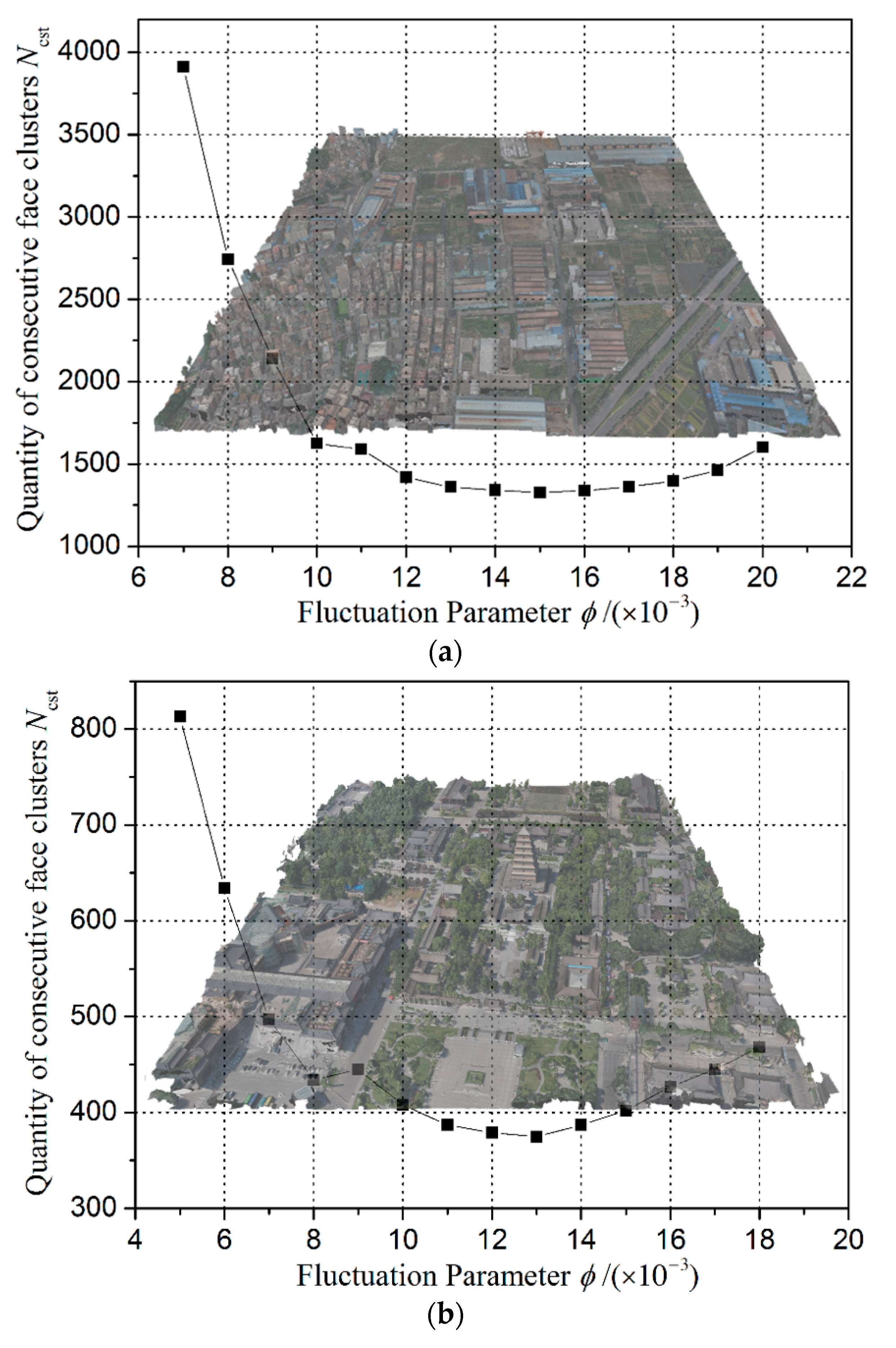
After obtaining the threshold of the fluctuation parameter, confirmation of is divided into two steps. First, the relation between the corresponding vertices and is determined, with as the independent variable, and its corresponding vertices are determined by their weights. The weight of a vertex is calculated by the area sum of the triangular faces , and the calculated vertex is the convergence vertex. Each value of refers to the interval . Similar to the study in Ref. [33], the interval is defined as 0.001. Figure 3 displays the relation between the fluctuation parameter and the weight of the vertices of the input surfaces of scenery 1 (vertices: 1,623,876; faces: 3,145,277) and scenery 2 (vertices: 1,233,187; faces: 2,392,672).
After the extraction of planar vertices, their adjacent faces and edges are recognized as planar. From the relation between weighted vertices and the fluctuation parameter , the threshold of the fluctuation parameter is confined to the second quasi-zero interval.
Ascertaining relies on the second step of this research, which is determining the relation between the quantity of consecutive surface clusters of planar surfaces and . When is less than the proper value, consecutive surface clusters are divided within the planar surfaces. When is larger than the proper value, occasional clusters appear that are mostly located at vegetation. However, the surfaces adopted must be large enough to allow occasional clusters to appear. Otherwise, there will be more than one that corresponds to the minimum , which is . Figure 4 displays this relation for the input surfaces of scenery 1 and scenery 2. Each value of is assumed to have the threshold in Figure 4 to find the corresponding .
In theory, the second step is enough to Figure out , but conformity between the two steps guarantees the reliability of . Supposing quasi-zero intervals are defined when the weight of weighted vertices is , it is not a parameter with strict standards, because the second step provides dual verification. In the experiments of this article, = 0.01. Figure 5 displays of scenery 1 and scenery 2 at all levels of simplification.
3.2. Extraction of Planar Surfaces
In accordance with the above extraction of planar vertices, methods to extract planar surfaces are as follows:
- Dihedral angles of edges: This method is frequently applied when the edges directly link two adjacent faces. When the dihedral angle of edges (maximum: ) is larger than the threshold of the dihedral angle set, the two faces that share the corresponding edge are recognized as planar ones. The calculation of the dot products of normal vectors determines the dihedral angles of edges.
- Recognition of planar vertices: Planar vertices are recognized by using the threshold of fluctuation parameter obtained above.
- Recognition of planar vertices with extension: Building on the basis of the recognition of planar vertices, the average dihedral angle of the edges of the recognized planar surfaces is calculated, and the average angle is regarded as the threshold of dihedral angles. All sub-planar edges are traversed until all the dihedral angles of sub-planar edges are larger than the threshold.
Definition 3.
Sub-planar geometric elements are vertices and edges located at the borders of the consecutive surface clusters of planar surfaces. A vertex is recognized as sub-planar when at least two of its directly linked edges are recognized as sub-planar. They are renewed when implementing the extension.
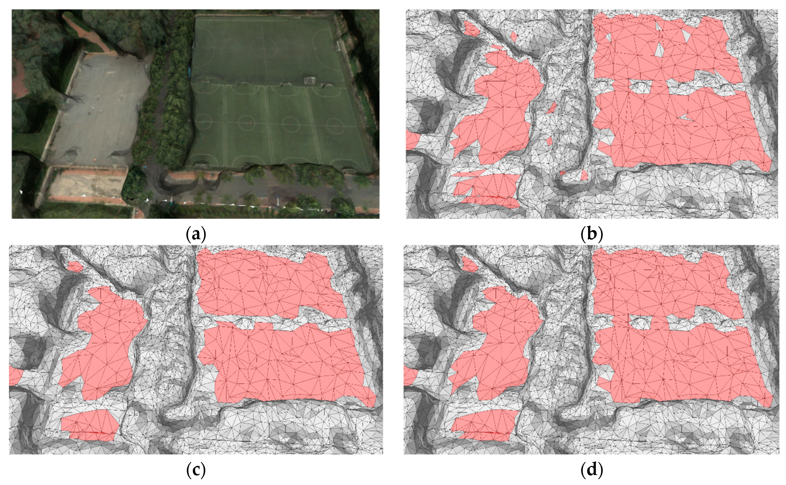
Figure 6 displays the recognition effects resulting from three methods for extracting planar surfaces from input surfaces. It is clear that extracting planar surfaces according to only dihedral angles causes the division of consecutive surface clusters within the planar surfaces and the occasional clusters located at vegetation simultaneously. Without extension, the narrow planar channels of planar surfaces without planar vertices fail to be extracted. It is obvious that the recognition of planar vertices with extension is an optimal choice for extracting planar surfaces. The threshold of dihedral angles is the average of recognized edges’ dihedral angles through the recognition of planar vertices in Figure 6b,d.
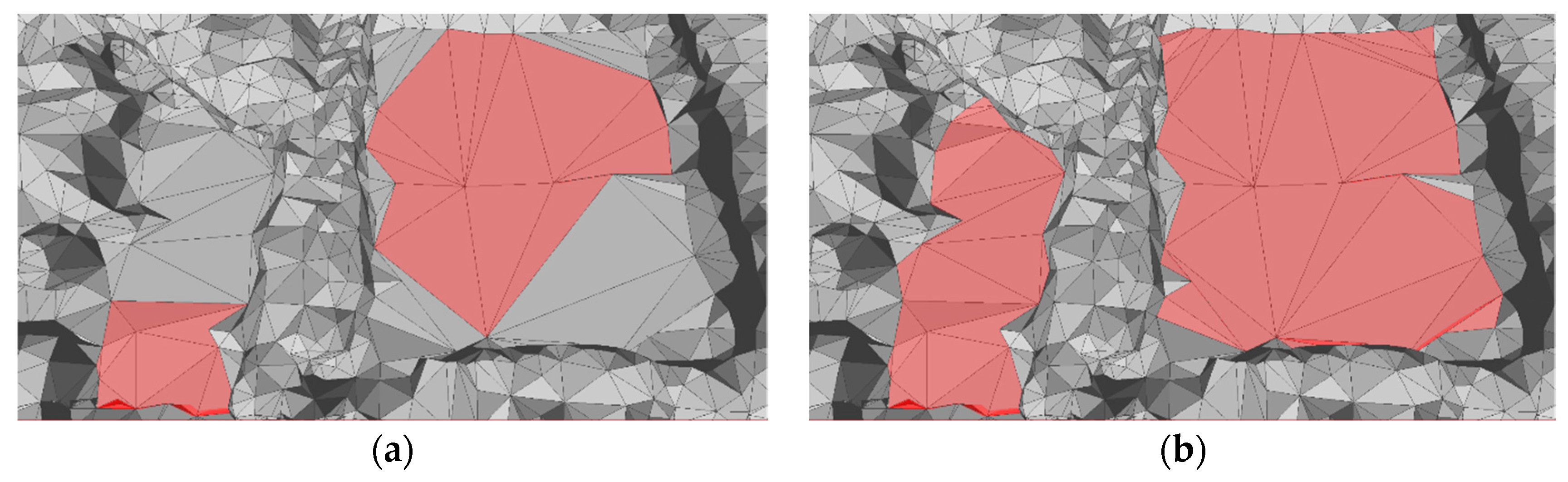
For simplified surfaces, because of the decrease in the threshold , the proportion of planar faces determined through planar vertices decreases, so the faces of consecutive surface clusters without any planar vertices appear much more often, as shown in Figure 7.
Therefore, experiments are needed to determine the most suitable methods for planar surface extraction. The number of consecutive surface clusters of planar surface extraction was compared with the surfaces simplified by using the dihedral angles of edges as rulers. As shown in Figure 4, extracted planar surfaces based on input surfaces, which is the most precise approach, contain 1329 and 375 consecutive surface clusters, respectively. The threshold of dihedral angles is also the average of edges’ dihedral angles recognized through the identification of planar vertices. As shown in Figure 8, when the simplification rate is higher or the LOD level is lower than the elbow points, method 1 is adopted to extract planar surfaces.
In summary, method 3 is suitable for input surfaces and those with a comparably low simplification rate, which can also be determined by the number of consecutive surface clusters. When the simplification rate increases, method 1 is adopted using the average of dihedral angles as the threshold obtained from method 2. Determining the threshold that will be used for identifying the method that ought to be used is also solved in this subsection.
3.3. Extraction of Urban Frameworks
The purpose of the extraction is to measure the ability of simplification algorithms to maintain urban frameworks. This goal can be realized by defining urban frameworks as sub-planar edges and vertices after the extraction of planar surfaces. The extraction focuses on sub-planar edges, of which the most significant are infrastructural borders, especially the borders of buildings. Therefore, the borders of buildings should manifest as edges, rather than low-quality faces [39], but input surfaces and surfaces with a low simplification rate usually manifest as low-quality faces [28]. Therefore, the simplification rate is the basis of such extraction. Here, the concept of the visual face is introduced before discussing the experiments.
In this stage of the extraction, some sub-planar edges may be linked to just one sub-planar vertex. This phenomenon is an outlier, which is eliminated while extracting urban frameworks.
Definition 4.
A Virtual face is not an actual triangular face. It is a portion of a sub-planar edge, thus adding a condition that two faces sharing an edge belong to two different planar consecutive surface clusters. Because such edges are regarded as a face with the sampling method described in Section 4, they are referred to as faces rather than edges.
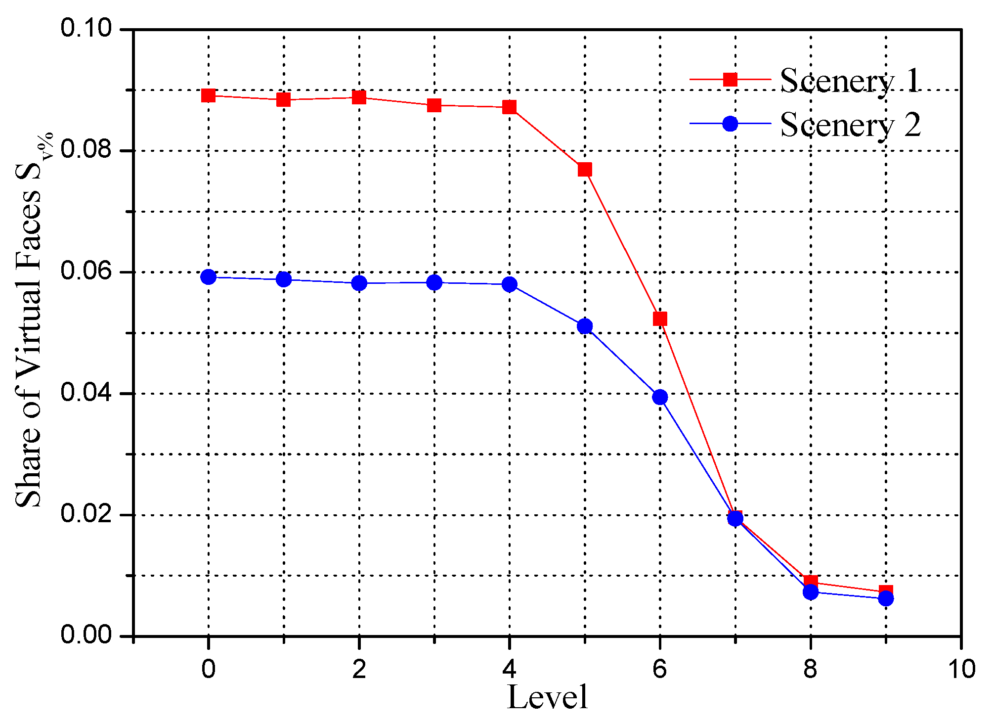
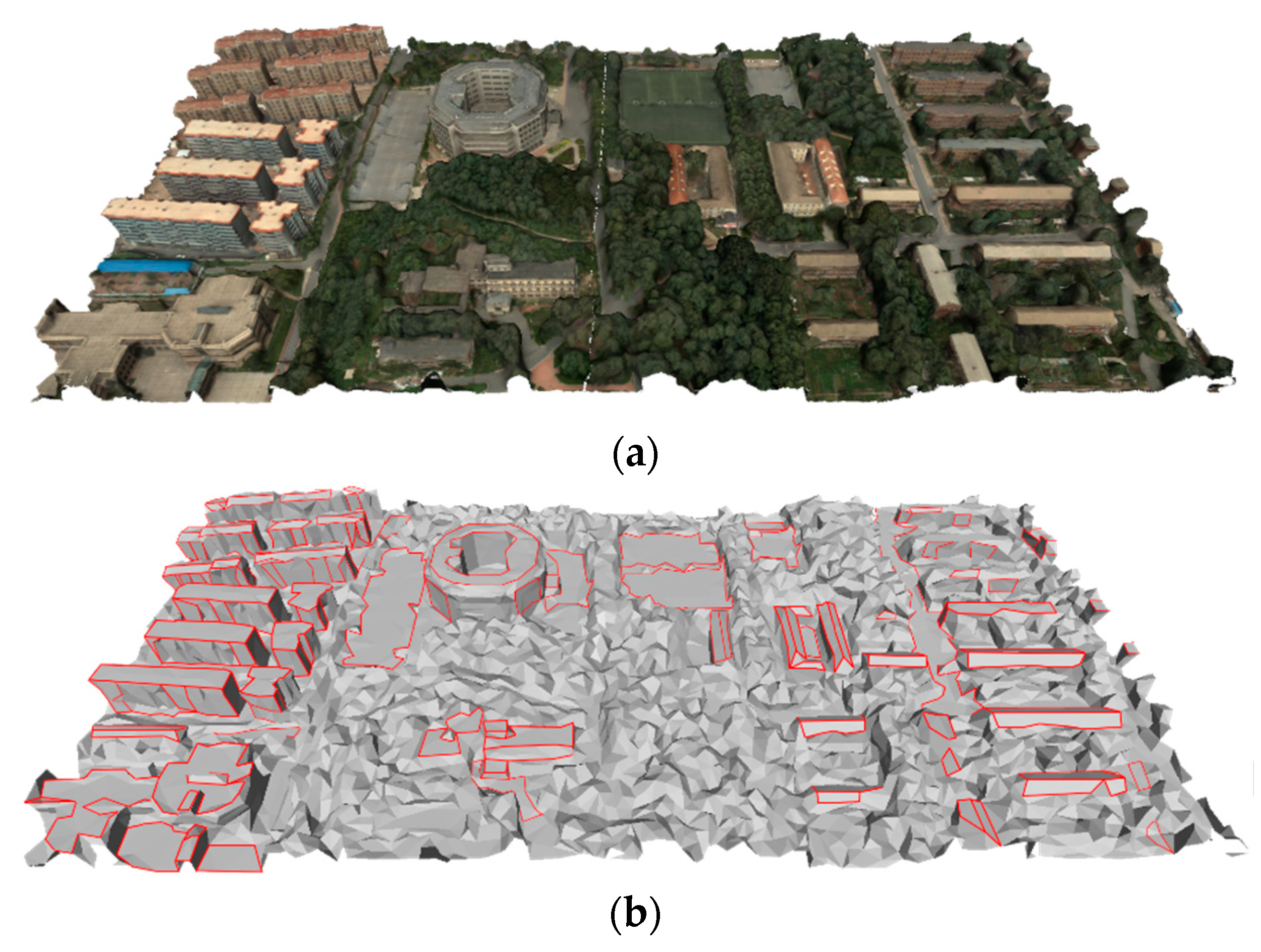
The proportion of virtual faces compared with all detailed surfaces is assumed to be large and stable enough that the borders of buildings can be sufficiently recognized. Figure 9 shows experiments on for scenery 1 and scenery 2. The extraction of urban frameworks is only valid when the simplification rate is higher or the LOD level is lower than the turning points. Figure 10 exemplifies the effect of extracted urban frameworks.
4. Sampling
As in Metro, converting the surface distance measurements (infinite continuous data) into point-to-plane distances (finite discrete data) is the basic approach to such measurements. The tool used in our research is a new version of POV ray-tracer [40], providing an efficient method to measure point-to-surface distances.
The weights of the sampling points are set to be equal for the error measurement of detailed surfaces, while those for the error measurement of urban frameworks visually highlight the conspicuousness. The importance of the frameworks of detailed surface sampling is emphasized by introducing virtual faces.
4.1. Detailed Surfaces
For input surfaces, the urban framework is likely to be TINs with low quality [21]. Detailed surface assessment is assumed to highlight urban frameworks, so our sampling was based on the perimeter of faces, with virtual ones supplemented as an extension.
Architectural borders are also more accurate compared with other objects with similar RGB values, such as vegetation. Even if the RGB values are similar, as a result of partial spectral reflection, the surfaces surrounding such surfaces are fairly accurate. Therefore, the framework is both significant and accurate. Using the perimeter as a sampling index enables the upgrade of the weights of borders.
The balance of sampling was maintained by adopting a method based on the centroid of edges and faces, as shown in Figure 11.
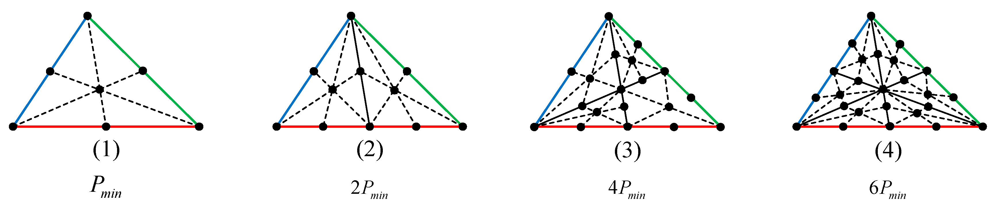
In this operation, sub-planar edges, which are common elements of different planar faces, are of great significance for maintaining the urban framework. Therefore, such edges serve as edges and virtual faces at the same time. The length of these edges is multiplied by a coefficient as the perimeter of virtual faces for face sampling. If the corresponding number of sampling points in a virtual face is , then the sampling points are located at quantiles. Setting is similar to the sampling of low-quality TINs along infrastructural borders. All vertices are part of the sampling, so the decision to be made is the weight of the vertices when conducting error measurement.
A sampling indicator based on perimeters is optimal for detailed surfaces, while sampling planar ones is not ideal because virtual faces are not under consideration. The area of triangular faces is adopted in the sampling of planar surfaces, and this is the approach used in Metro. The error of planar surfaces is not included in our assessment methods, but it highlights the logic of assessment indexes.
4.2. Urban Frameworks
In contrast to detailed surfaces, urban frameworks only consist of edges, and all vertices of urban frameworks are sampled. The sampling points of edges are distributed according to their length, with standardized sampling points. The relation between sub-planar edge length and sampling points is
in which is the edge being sampled, and is the average length of the edges of urban frameworks. A sampling density similar to that in Metro is established by setting to 8.
However, different emphases are placed on different sampling points. More emphasis should be placed on the borders of buildings, which are virtual faces. The larger the curvature of a sub-planar edge, the more emphasized it should be. The weight of the sampling points on the edges is
in which is the dihedral angle of the corresponding edge, and is a coefficient. If the corresponding edge is a virtual face, then is set to 2. Otherwise, it is set as 1. and represent the two emphases mentioned above.
If a sampling point on a vertex is adjacent to just two sub-planar edges, the weight is the average of those on the edges. If it is adjacent to more than two sub-planar edges, the weight is
where the coefficient is set to highlight the corners of buildings. It can be set according to the subjective precision needed for the building corners. In the experiments of this article, was set to 1.
5. Assessment Implementation
5.1. Assessment Indexes
In this context, the errors of planar surfaces, detailed surfaces, and urban frameworks can be measured. In addition, numerical indexes were designed, as listed below.
- Mean error of planar surfaces: The sampled surface serves as the pivot (sampled) surface [20], and the mean error is obtained by measuring the sampling points of different types of surfaces, which are classified in Section 3. For measuring the mean error of detailed and planar surfaces, input surfaces serve as the only pivot surfaces because the aim is to pick a larger error, and this mean error is larger than that in Metro [20]. Metro adopts dual measurement to obtain the Hausdorff distance, which was not used in our studies. For measuring the mean error of urban frameworks, simplified surfaces are used as the pivot surfaces, as explained in Section 4.
- Planarity indicator : Most planar surfaces in urban models can be seen as entirely planar after simplification because of the limited precision of 3D reconstruction [28]. This concept is expressed numerically here. Specifically, the larger the value of , the more satisfactory the planar surfaces.
The length of the planar edge is , and the sum is added as a weight to calculate planarity. and are unit normal vectors of the two adjacent faces of the edge being calculated, and is the number of planar edges.
- Proportion of faces among detailed surfaces : This index is the proportion of the faces among detailed surfaces compared with all the surfaces. A larger value of implies that more geometric elements are located on detailed surfaces, which is likely conducive to the preservation of surface and indicating areas for improvement. A larger also implies fewer geometric elements for planar surfaces, which corresponds to a larger in most cases because planarity is accurately achieved with fewer faces, as illustrated in Figure A1c (Appendix A).
- Error disparity of detailed surfaces : The error disparity is fundamental for exploring areas for improving simplification algorithms, and it is independent of comprehensive errors. Larger numerical errors of detailed surfaces are not equivalent to failures. When the error of detailed surfaces is larger than its own comprehensive error, the simplification algorithm is worth further exploring. If the errors of detailed and planar surfaces are and , respectively, and the comprehensive error measured by Metro is , then
If is small, improvement can be realized by combining with other algorithms, such as aQSlim, or it identifies and area for improvement that is worthy of in-depth studies. Fundamentally, it facilitates an in-depth understanding through self-comparison.
- The gap between errors from different simplification algorithms : This is for more precise analyses when the disparity of different error measurements is too small to conduct accurate analyses. In (8), symbolizes the mean error of the type of surfaces classified at the same simplification rate.
All the numerical indexes above were calculated during the surface division process described in Section 3 and the sampling process in Section 4. All of these indexes are calculated directly on the basis of the length of the scenery. For example, the side length of the pedestal of the Greater Wild Goose Pagoda in scenery 1 is 77.684 m, while the actual length is 25.500 m. Therefore, the unit of error of details and frameworks is the virtual length.
5.2. Implementation
Before the implementation of surface classification, sampling, and the index measurement proposed above, the proper format of 3D surfaces, including the position of vertices, unit normal of every triangular face, and the edges and faces containing two and three vertices, needs to be ensured. The format we adopted is .obj, which meets the demands mentioned above [41]. The implementation is shown in Algorithm 1.
| Algorithm 1. Implementation of multifaceted geometric assessment for simplified urban surfaces built by 3D reconstruction. The process determines the method to use for planar surface extraction and whether to implement extraction and mean error measurement of urban frameworks. | |
| Assessment Based on Surface Classification | |
| 1 | Insert (1x.obj, 2x.obj); bool fluct, frmk /*1x.obj is the input surface */ |
| 2 | 1x.obj, 2x.obj /*Obtain Fluctuation parameter */ |
| 3 | Weight_vt 1x.obj, 2x.obj /*Obtain weight of each vertex */ |
| 4 | [<=] 1x.obj, 2x.obj /*Obtain number of consecutive surface clusters and is the independent variable */ |
| 5 | = findthresholdFluct (, Weight_vt, [<=]) |
| 6 | () 2x.obj /*Test for choice of classification method */ |
| 7 | Obtain proportion of virtual faces compared with all the detailed surfaces |
| 8 | cin >> fluct; cin >> frmk /* Judge the best way to extract planar surfaces and whether to extract urban frameworks, as illustrated in Figure 8 and Figure 9 */ |
| 9 | iffluct == true then /* Recognition of planar vertices with extension is adopted */ |
| 10 | Planar_vt ≤ |
| 11 | Sub_planar_expand () /*Extraction using method 3 */ |
| 12 | end |
| 13 | iffluct == false then /* Dihedral angles of edges are adopted */ |
| 14 | Planar_extract () /* Extraction using method 1 */ |
| 15 | end /* Sub-planar edges and virtual faces are also obtained */ |
| 16 | Obtain planarity of planar surfaces |
| 17 | Obtain face share of detailed surfaces |
| 18 | Sample detailed surfaces (1x.obj) |
| 19 | Measure mean error of detailed surfaces |
| 20 | Obtain error disparity of detailed surfaces |
| 21 | iffrmk == true then /*Implement extraction and mean error measurement of urban frameworks */ |
| 22 | Sample sub-planar edges and calculate weight of sampling points (1x.obj) |
| 23 | Measure mean error of urban frameworks |
| 24 | end |
| 25 | return |
Determination of the method to use is based on and (lines 6, 7), and users are then able to identify the optimal means of extracting planar surfaces and whether to extract and measure the error of urban frameworks (line 8). Lines 9–20 are responsible for obtaining the indexes correlated to the classification of detailed and planar surfaces. The indexes for urban frameworks are implemented in lines 21–24.
6. Experiments and Discussions
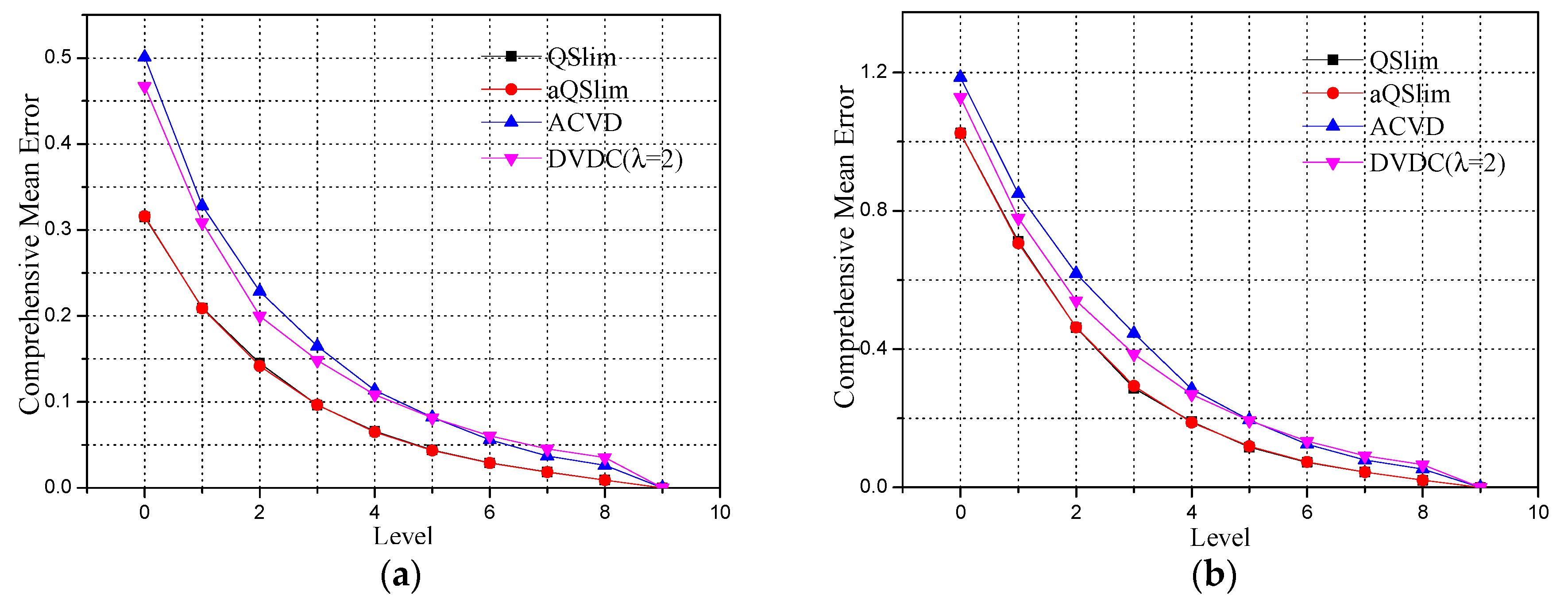
Before the description of the experiments in our methods, the mean error measured by the tool Metro for scenery 1 (a) and 2 (b) is shown in Figure 12. The value measured by Metro is the comprehensive error of the whole surface, and the performance is not satisfactory.
6.1. Error Measurement
Figure 13 displays the error of detailed and planar surfaces. It is noticeable that surface detail preservation is the core of surface simplification. This viewpoint has been stressed in almost all reports on this subject. It is clear that the mean error of detailed surfaces is able to assess simplification algorithms in higher resolution. Logically, the error of planar surfaces is determined in a different manner.
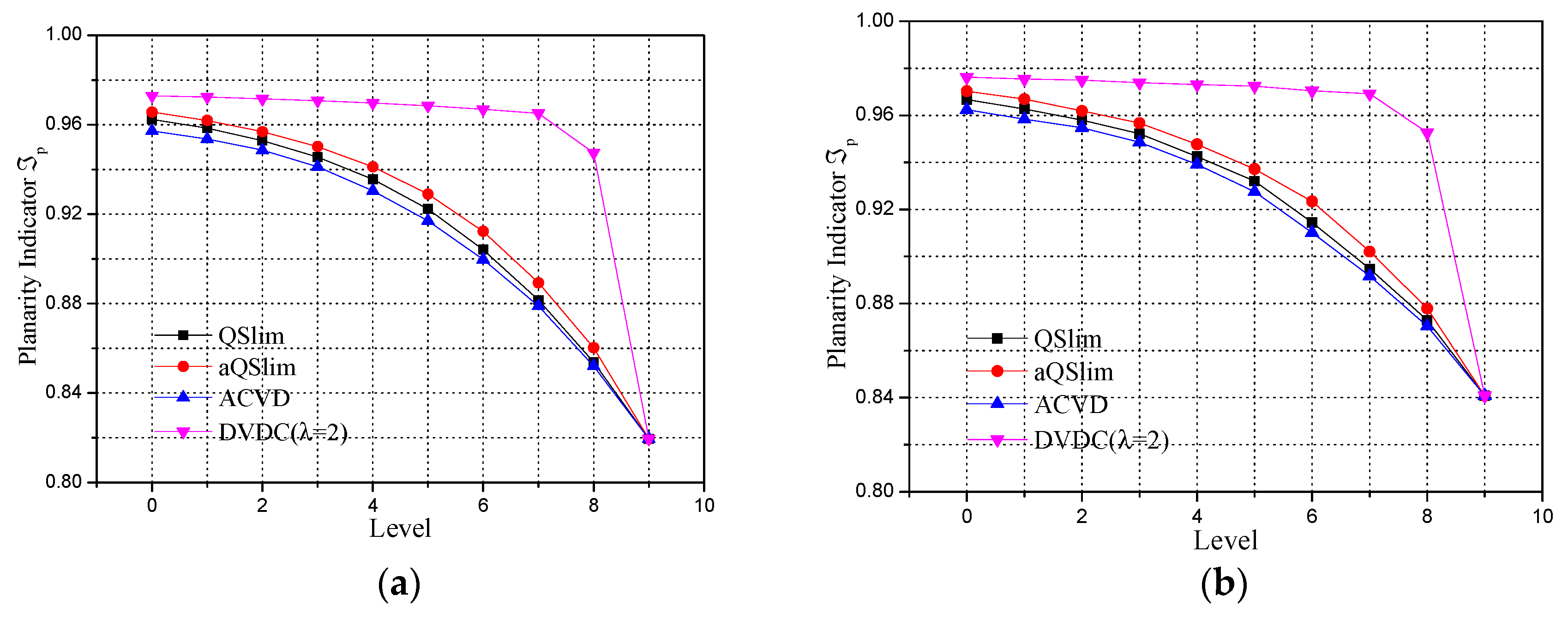
However, as mentioned above, the planarity of planar surfaces represents the quality of our assessment instead of its error relative to input surfaces. Therefore, the planarity of planar surfaces is represented by , as shown in Figure 14.
From the comprehensive error, as well as errors of detailed and planar surfaces, it can be concluded that ACVD and DVDC () are inferior and not worth further studying. However, DVDC () performs much better for the planarity of planar surfaces. The following explorations are based on this observation.
6.2. Improvement through Combination
The planarity of planar surfaces is meaningful only if the errors of simplified surfaces are low. The main considerations for assessing room for improvement of simplification algorithms are whether more geometric elements are placed on detailed surfaces and whether the error of detailed surfaces is low compared with its own comprehensive error. Therefore, the proportion of faces of detailed surfaces and the error disparity of detailed surfaces are incorporated to design a combination of simplification algorithms.
As shown in Figure 15, when there is disagreement between the real value of the mean error and the above two factors, especially the disparity of detailed surfaces, it indicates the area for improvement. Specifically, a higher indicates that more geometric information (faces) is gathered to support detailed surfaces, and lower indicates better preservation of detailed surfaces compared with its own comprehensive error. Both ACVD and DVDC implement the simplification of reorganized surfaces, while the other two simply make modifications based on the input surfaces. The large changes in , , and when the simplification rate is low represent the characteristics of different surface simplification algorithms. The indexes facilitate a more intuitive understanding of the simplification.
It is also revealed that aQSlim and QSlim remain stable in terms of the disparity of detailed surfaces. Therefore, it is logical to assume that the combination of an excellent at a low simplification rate and a stable and relatively small applied throughout the whole simplification rate. Therefore, an improvement scheme is offered as follows:
- Choose the lowest simplification rate at DVDC, which is the same number of vertices as the input surfaces for so-called simplification. This procedure is also named remeshing [42].
- Implement edge collapse through aQSlim.
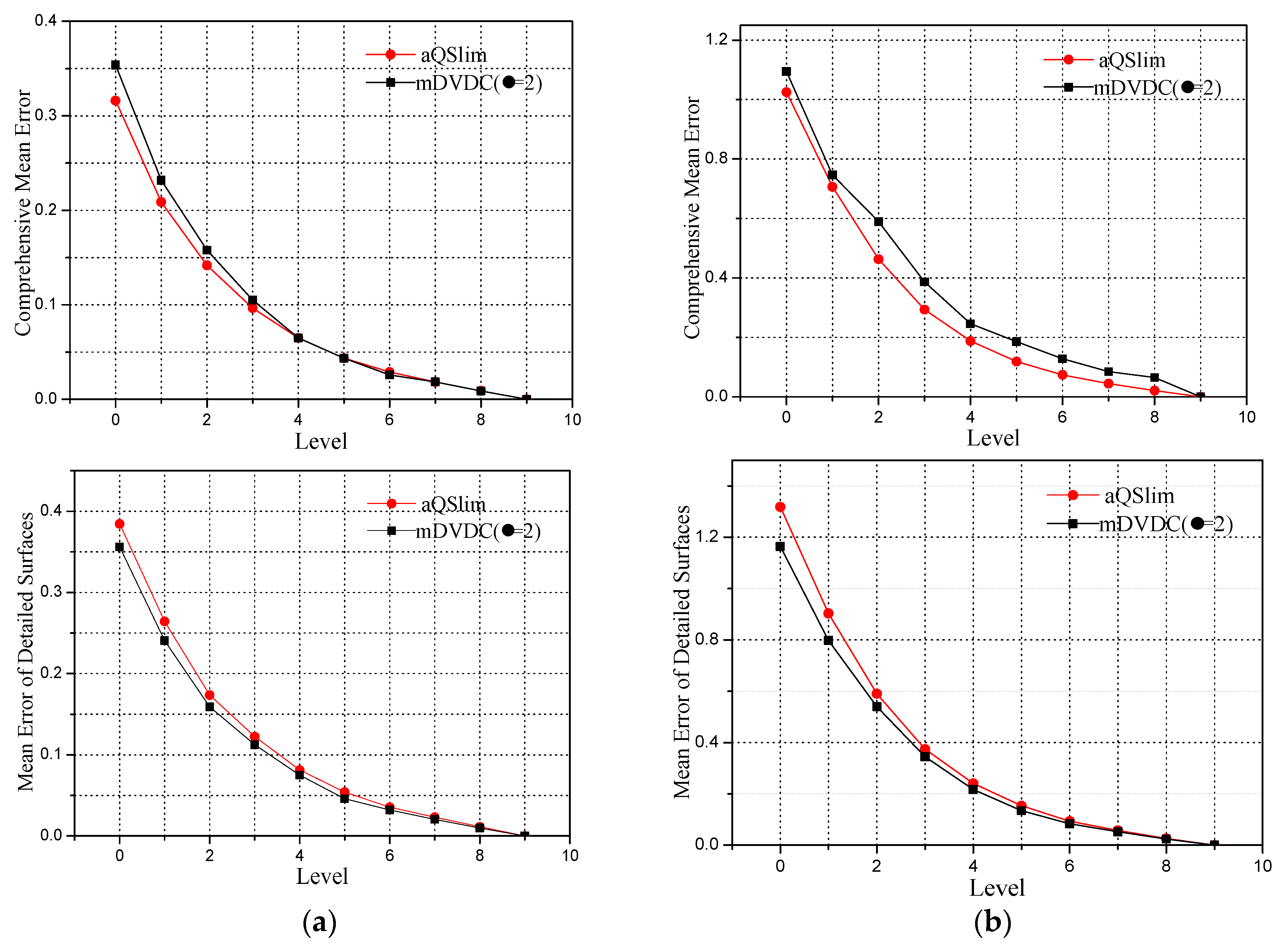
The property of the modified DVDC (mDVDC) is measured in terms of the mean error of all surfaces and detailed surfaces, as shown in Figure 16.
In all the experiments conducted, the error of urban frameworks is consistent with that of detailed surfaces. However, when studying the optimal choice of the curvature indicator , they perform slightly differently, which is explored in the following.
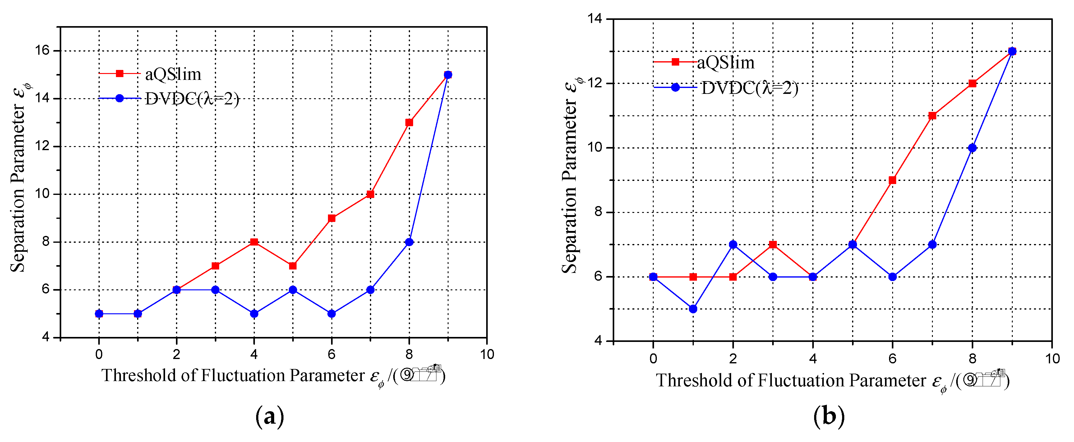
6.3. Choice of Optimal Parameter
As analyzed above, the extraction of urban frameworks is valid from level 4 to 0. Moreover, the effects at a high simplification rate are of greater significance because it indicates that the correct choice of variable parameters does not significantly influence the simplification effects. Experiments on the optimal parameter are limited to levels 4–0. The experiment included the gap of errors for different simplification algorithms to test the errors of detailed surfaces and urban frameworks in terms of selecting the optimal . The default and are mDVDC (optimal ) and mDVDC (second optimal ), respectively. The second optimal corresponding to is the second lowest error of detailed surfaces or urban frameworks. Table 1 and Table 2 show the test results of tile A (Figure A2) and tile B (Figure A3) respectively extracted from scenery 1 and 2.
The improved simplification algorithm mDVDC is still better at preserving detailed surfaces and urban frameworks. Because reorganizing surfaces is much more time-consuming than performing modifications on the basis of input surfaces, such as in edge collapse [43], it is necessary to choose the optimal variable parameters for simplification algorithms using surface reorganization. From the two tables above, although the choice of the optimal is mostly consistent, it can be clearly seen that the mean error of urban frameworks is better at obtaining the optimal choice of . As a result of the extremely small , it is extremely difficult to obtain the optimal variable parameters without numerical error measurement. Moreover, urban frameworks are usually more important for the simplification of urban surfaces, as mentioned above. In sum, the mean error of urban frameworks is more appropriate than that of detailed surfaces for obtaining the optimal variable parameters.
6.4. Time Property
All the results presented in this paper were conducted on a PC with Intel i5-4210M, 2.6 GHz CPU, 8 GB memory, and a 64-bit Windows 7 operating system. This subsection compares the time performance of our method with that of Metro without building a coherent coloring scheme, using simplified surfaces at level 4. Because the error of the urban framework is not always applicable, the time property tests involved measurement without (lines 1–20 of Algorithm 1) and with the error of the urban framework (lines 1–25 of Algorithm 1). The tested surfaces include scenery 1 and 2, as well as tile A and tile B. Time performance testing has been delivered as shown in Table 3.
7. Conclusions
With an aim to assess the common 3D structure of computer graphics of simplified triangular surfaces built by 3D reconstruction using stereo aerial photographs, this article focuses on the quality assessment of simplified surfaces based on the classification of urban surfaces. The basic objective is to maintain the details of urban models, which are detailed surfaces and urban frameworks. The conclusions are listed below.
- Classification was achieved by extracting planar surfaces. For input surfaces, this study adopted weighted vertices and the number of consecutive surfaces, as well as their relations to fluctuation parameters, to determine the threshold of fluctuation parameters. Simplified surfaces based on the estimated number of consecutive surfaces of input surfaces is the proper method selected to extract planar surfaces. Given these comprehensive considerations, urban surfaces were classified accurately.
- The results of sampling the pivot surfaces reveal that the mean errors of detailed surfaces and urban frameworks were more capable of measuring the preservation capacity of simplified surfaces than the commonly used tool Metro.
- This article proposes indexes that are based on classification and go beyond measuring mean errors. Other indexes not only facilitate the in-depth understanding of simplification algorithms but also support the improvement of the quality of simplified surfaces through the easy combination of off-the-shelf simplification algorithms.
- The mean error of urban frameworks extracted from simplified surfaces not only meets the needs of framework preservation but is also stable in its determination of the optimal variable parameter of simplification algorithms for some urban surfaces.
In summary, this article reports the multifaceted geometric assessment for simplified urban surfaces built by 3D reconstruction. Future explorations include an objective assessment of newly developed simplification algorithms for simplifying urban models, as well as examining the almost countless combinations of off-the-shelf algorithms to develop modified simplification methods for urban models in a much easier manner.
Author Contributions
In addition to the overall contribution, S.L. conceived the ideas and concepts and was responsible for the writing. H.Y. helped process the experimental data. X.C. was responsible for the administration and funding of this research. D.W. reorganized the experimental results and expressions in the article. W.J. contributed to the linkage of open-source POV-Ray.
Funding
National 863 Program: 2015AA7031093C.
Acknowledgments
We are grateful to Xi’an Research Institute of Survey and Mapping for providing 3D surfaces, which are the result of the Provincial Exploration Project (project ID: 7131145). This study is funded by National 863 Program (project ID: 2015AA7031093C). This research received no external funding.
Conflicts of Interest
All authors declare no conflict of interest. The material provider declares no financial stake in this research. The funding is a national program that supports research without any financial interest.
Appendix A
The appendix displays samples of experimental results using the simplification algorithms mentioned above. It is shown to prove the surface simplification quality and to highlight the significance of our work. All the content is referenced in the article.
Figure A1.
A tile extracted from scenery one. Simplified surfaces are both at level 7. DVDC () seems better than aQSlim for its high simplification rate and greater planarity at planar surfaces and detailed surfaces with more geometric elements. Therefore, there is an urgent need to create numerical analyses for such observations, based on which we launched the research in this article. (a) Input surface with texture; (b) aQSlim; (c) DVDC ().

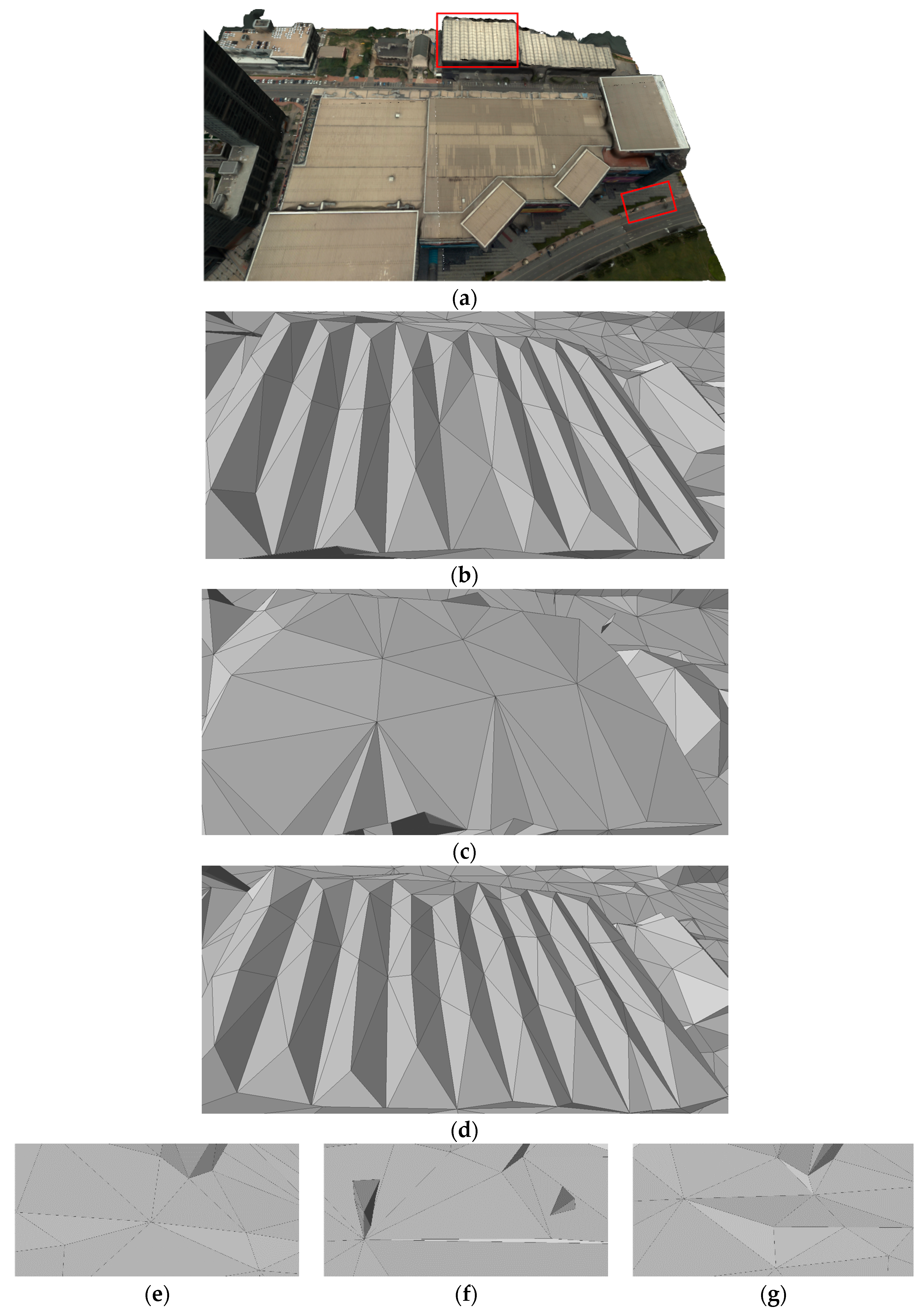
Figure A2.
Simplification results at level 2 of tile A. Both regions circled in red in (a) are simplified, as shown in the others. There are some differences, similar to Figure 1: mDVDC () performs better than (d), while DVDC () performs better than (f). Therefore, this article helps solve the problem of deciding on the best algorithms through observation. (a) Input surface with texture; (b) aQSlim; (c) DVDC (); (d) mDVDC (); (e) aQSlim; (f) DVDC (); (g) mDVDC ().

Figure A3.
Simplification results at level 2 of tile A. The other simplification results are displayed in Figure 1. (a) Input surface with texture; (b) ACVD; (c) DVDC ().
Figure A3.
Simplification results at level 2 of tile A. The other simplification results are displayed in Figure 1. (a) Input surface with texture; (b) ACVD; (c) DVDC ().

References
- Nash, C.; Williams, C.K.I. The shape variational autoencoder: A deep generative model of part-segmented 3D objects. Comput. Graph. Forum 2017, 36, 1–12. [Google Scholar] [CrossRef] [Green Version]
- Jackson, B.; Jelke, B.; Brown, G. Yea Big, Yea High: A 3D User Interface for Surface Selection by Progressive Refinement in Virtual Environments. In Proceedings of the 25th IEEE Conference on Virtual Reality and 3D User Interfaces (VR), Reutlingen, Germany, 18–22 March 2018; pp. 320–326. [Google Scholar]
- Jung, J.W.; Lee, J.S.; Cho, D.W. Computer-aided multiple-head 3D printing system for printing of heterogeneous organ/tissue constructs. Sci. Rep. 2016, 6, 21685. [Google Scholar] [CrossRef] [PubMed]
- Gong, J.; Cui, K.; Zhang, W.; Ding, Y.; Huang, B.; Lu, Y.; Wang, J. Design and realization of active infrared imaging system based on power-over-fiber technique. Opt. Rev. 2018, 25, 517–522. [Google Scholar] [CrossRef]
- El-Asha, S.; Zhan, L.; Iungo, G.V. Quantification of power losses due to wind turbine wake interactions through SCADA, meteorological and wind LiDAR data. Wind Energy 2017, 20, 1823–1839. [Google Scholar] [CrossRef]
- Arashpour, M.; Heidarpour, A.; Akbar Nezhad, A.; Hosseinifard, Z.; Chileshe, N.; Hosseini, R. Performance-based control of variability and tolerance in off-site manufacture and assembly: Optimization of penalty on poor production quality. Constr. Manag. Econ. 2019, 1–13. [Google Scholar] [CrossRef]
- Biljecki, F.; Stoter, J.; Ledoux, H.; Zlatanova, S.; Çöltekin, A. Applications of 3D City Models: State of the Art Review. ISPRS Int. J. Geogr. Inf. 2015, 4, 2842–2889. [Google Scholar] [CrossRef] [Green Version]
- Wang, A.; An, N.; Zhao, Y.; Iwahori, Y.; Kang, R. 3D Reconstruction of Remote Sensing Image Using Region Growing Combining with CMVS-PMVS. Int. J. Multimed. Ubiquitous Eng. 2016, 11, 29–36. [Google Scholar] [CrossRef]
- Zhao, Y.; Liu, Y. Patch based saliency detection method for 3D surface simplification. In Proceedings of the 21th International Conference on Pattern Recognition, Tsukuba, Japan, 11–15 November 2012; pp. 845–848. [Google Scholar]
- Holzmann, T.; Maurer, M.; Fraundorfer, F.; Bischof, H. Semantically Aware Urban 3D Reconstruction with Plane-Based Regularization. In Proceedings of the 15th European Conference on Computer Vision (ECCV), Munich, Germany, 8–14 September 2018; pp. 468–483. [Google Scholar]
- Ran, M.; Xiao, S.; Zhou, X.; Xiao, W. Asphalt Pavement Texture 3D Reconstruction Based on Binocular Vision System with SIFT Algorithm. In Proceedings of the International Conference on Smart Grid & Electrical Automation, Changsha, China, 27–28 May 2017; pp. 213–218. [Google Scholar]
- Bacharidis, K.; Sarri, F.; Paravolidakis, V.; Ragia, L.; Zervakis, M. Fusing Georeferenced and Stereoscopic Image Data for 3D Building Façade Reconstruction. ISPRS Int. J. Geogr. Inf. 2018, 7, 151. [Google Scholar] [CrossRef]
- Islam, M.B.; Wong, L.K.; Low, K.L.; Wong, C.O. Warping-based Stereoscopic 3D Video Retargeting with Depth Remapping. In Proceedings of the 2019 IEEE Winter Conference on Applications of Computer Vision (WACV), Hilton Waikoloa Village, HI, USA, 7–11 January 2019; pp. 1655–1663. [Google Scholar]
- Biasotti, S.; Thompson, E.M.; Barthe, L.; Berretti, S.; Giachetti, A.; Lejemble, T.; Tortorici, C. Recognition of geometric patterns over 3D models. In Proceedings of the 11th Eurographics Workshop on 3D Object Retrieval, Eurographics Association, Delft, The Netherlands, 16 April 2018; pp. 71–77. [Google Scholar]
- Wang, X.; Burghardt, D. A Mesh-Based Typification Method for Building Groups with Grid Patterns. ISPRS Int. J. Geogr. Inf. 2019, 8, 168. [Google Scholar] [CrossRef]
- Goesele, M.; Snavely, N.; Curless, B.; Hoppe, H.; Seitz, S.M. Multi-view stereo for community photo collections. In Proceedings of the IEEE 11th International Conference on Computer Vision, Rio de Janeiro, Brazil, 14–21 October 2007; pp. 1–8. [Google Scholar]
- Fuhrmann, S.; Langguth, F.; Goesele, M. MVE: A multi-view reconstruction environment. In Proceedings of the 12th Eurographics Workshop on Graphics and Cultural Heritage, Eurographics Association, Darmstadt, Germany, 6–8 October 2014; pp. 11–18. [Google Scholar]
- Furukawa, Y.; Curless, B.; Seitz, S.M.; Szeliski, R. Towards Internet-scale multi-view stereo. In Proceedings of the 23th Computer Vision and Pattern Recognition, San Francisco, CA, USA, 13–18 June 2010; pp. 1434–1441. [Google Scholar]
- Altantsetseg, E.; Khorloo, O.; Matsuyama, K.; Konno, K. Complex hole-filling algorithm for 3D models. In Proceedings of the 34th Computer Graphics International Conference, Yokohama, Japan, 27–30 June 2017; pp. 1–6. [Google Scholar]
- Cignoni, P.; Rocchini, C.; Scopigno, R. Metro: Measuring Error on Simplified Surfaces; Computer Graphics Forum: Oxford, UK; Blackwell Publishers: Hoboken, NJ, USA, 1998; Volume 17, pp. 167–174. [Google Scholar]
- Yao, L.; Huang, S.; Xu, H.; Li, P. Quadratic Error Metric Mesh Simplification Algorithm Based on Discrete Curvature. Math. Probl. Eng. 2015, 2015, 1–7. [Google Scholar] [CrossRef]
- Zhou, Y.F.; Zhang, C.; He, P. Feature preserving mesh simplification algorithm based on square volume measure. Chin. J. Comput. 2009, 32, 203–212. [Google Scholar] [CrossRef]
- Liu, S.; Ferguson, Z.; Jacobson, A.; Gingold, Y.I. Seamless: Seam erasure and seam-aware decoupling of shape from mesh resolution. ACM Trans. Graph. 2017, 36, 1–216. [Google Scholar] [CrossRef]
- Garland, M.; Heckbert, P.S. Surface simplification using quadric error metrics. In Proceedings of the 24th Annual Conference on Computer Graphics and Interactive Techniques, Los Angeles, CA, USA, 3–8 August 1997; ACM Press/Addison-Wesley Publishing Co.: New York, NY, USA, 1997; pp. 209–216. [Google Scholar] [Green Version]
- Liu, Y.J.; Xu, C.X.; Fan, D.; He, Y. Efficient construction and simplification of Delaunay meshes. ACM Trans. Graph. 2015, 34, 174. [Google Scholar] [CrossRef]
- Uccheddu, F.; Servi, M.; Furferi, R.; Governi, L. Comparison of Mesh Simplification Tools in a 3D Watermarking Framework. In International Conference on Intelligent Interactive Multimedia Systems and Services; De Pietro, G., Gallo, L., Howlett, R., Jain, L.C., Eds.; Springer: Gold Coast, Australia, 2018; pp. 60–69. [Google Scholar]
- Valette, S.; Chassery, J.M. Approximated Centroidal Voronoi Diagrams for Uniform Polygonal Mesh Coarsening; Computer Graphics Forum: Oxford, UK; USA Blackwell Publishing Inc.: Hoboken, NJ, USA, 2004; Volume 23, pp. 381–389. [Google Scholar]
- Salinas, D.; Lafarge, F.; Alliez, P. Structure-Aware Mesh Decimation; Computer Graphics Forum: Oxford, UK; USA Blackwell Publishing Inc.: Hoboken, NJ, USA, 2015; Volume 34, pp. 211–227. [Google Scholar]
- Nealen, A.; Igarashi, T.; Sorkine, O.; Alexa, M. Laplacian mesh optimization. In Proceedings of the International Conference on Computer Graphics & Interactive Techniques in Australasia & Southeast Asia, Kuala Lumpur, Malaysia, 29 November–2 December 2006; pp. 381–389. [Google Scholar]
- Wang, K.; Torkhani, F.; Montanvert, A. A fast roughness-based approach to the assessment of 3D mesh visual quality. Comput. Graph. 2012, 36, 808–818. [Google Scholar] [CrossRef]
- Zeineldin, R.A.; El-Fishawy, N.A. Fast and accurate ground plane detection for the visually impaired from 3D organized point clouds. In Proceedings of the 2016 IEEE SAI Computing Conference, London, UK, 13–15 July 2016; pp. 373–379. [Google Scholar]
- Maltezos, E.; Ioannidis, C. Automatic Extraction of Building Roof Planes from Airborne LIDAR Data Applying AN Extended 3d Randomized Hough Transform. ISPRS Ann. Photogramm. Remote Sens. Spat. Inf. Sci. 2016, 3, 209–216. [Google Scholar] [CrossRef]
- Sampath, A.; Shan, J. Segmentation and Reconstruction of Polyhedral Building Roofs from Aerial Lidar Point Clouds. IEEE Trans. Geosci. Remote Sens. 2010, 48, 1554–1567. [Google Scholar] [CrossRef]
- Valette, S.; Chassery, J.M.; Prost, R. Generic remeshing of 3D triangular meshes with metric-dependent discrete Voronoi diagrams. IEEE Trans. Vis. Comput. Graph. 2008, 14, 369–381. [Google Scholar] [CrossRef] [PubMed]
- Löwner, M.O.; Gröger, G.; Benner, J.; Biljecki, F.; Nagel, C. Proposal for a new LOD and multi-representation concept for CityGML. ISPRS Ann. Photogramm. Remote Sens. Spat. Inf. Sci. 2016, 4, 3–12. [Google Scholar] [CrossRef]
- Schmidt, R.; Singh, K. Meshmixer: An Interface for Rapid Mesh Composition. ACM SIGGRAPH 2010 Talks; ACM: Los Angeles, CA, USA, 2010; p. 6. [Google Scholar]
- Shuchat, A. Generalized Least Squares and Eigenvalues. Am. Math. Mon. 1985, 92, 656–659. [Google Scholar] [CrossRef]
- Cignoni, P.; Callieri, M.; Corsini, M.; Dellepiane, M.; Ganovelli, F.; Ranzuglia, G. Meshlab: An open-source mesh processing tool. In Proceedings of the Eurographics Italian Chapter Conference, Salerno, Italy, 2–4 July 2008; pp. 129–136. [Google Scholar]
- Frey, P.J.; Borouchaki, H. Surface mesh quality assessment. Int. J. Numer. Methods Eng. 1999, 45, 101–118. [Google Scholar] [CrossRef]
- POV-Ray-The Persistence of Vision Raytracer. Available online: http://www.povray.org/ (accessed on 17 August 2018).
- Isoda, Y.; Tsukamoto, A.; Kosaka, Y.; Okumura, T.; Sawai, M.; Yano, K.; Tanaka, S. Reconstruction of Kyoto of the Edo era based on arts and historical documents: 3D urban model based on historical GIS data. Int. J. Humanit. Arts Comput. 2009, 3, 21–38. [Google Scholar] [CrossRef]
- Pellerin, J.; Lévy, B.; Caumon, G.; Botella, A. Automatic surface remeshing of 3D structural models at specified resolution: A method based on Voronoi diagrams. Comput. Geosci. 2014, 62, 103–116. [Google Scholar] [CrossRef]
- Nießner, M.; Zollhöfer, M.; Izadi, S.; Stamminger, M. Real-time 3D reconstruction at scale using voxel hashing. ACM Trans. Graph. 2013, 32, 169. [Google Scholar] [CrossRef]
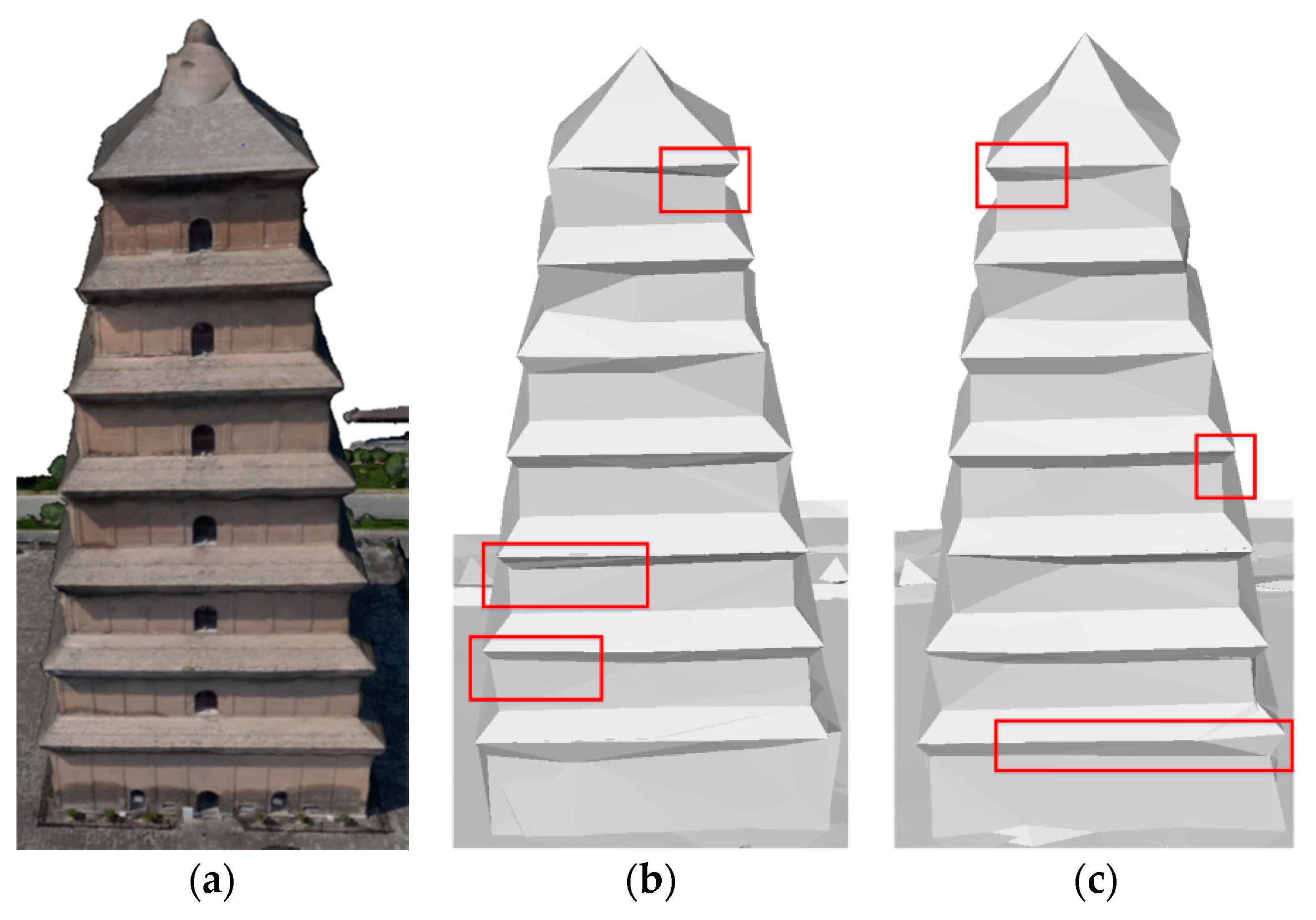
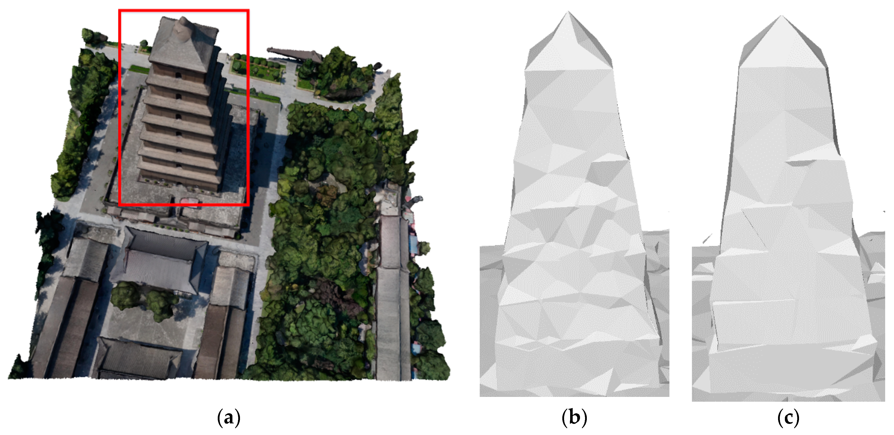
Figure 1.
The surface representation of the Greater Wild Goose Pagoda: (a) original surface with texture; simplified surface at level 0 simplified by (b) aQSlim and (c) mDVDC () (all explained in Section 2.3). The parts in the red rectangles perform better, so choosing which one is better is a dilemma.

Figure 2.
Effect of color mapping, a function of Metro [20]. It is clearly seen that major error is located on nonplanar surfaces for sharp features, such as the edges and corners of buildings. However, these urban frameworks are essential for the applications of urban surfaces, as mentioned above. (a) Input surfaces with texture; (b) Simplified surfaces after error mapping.
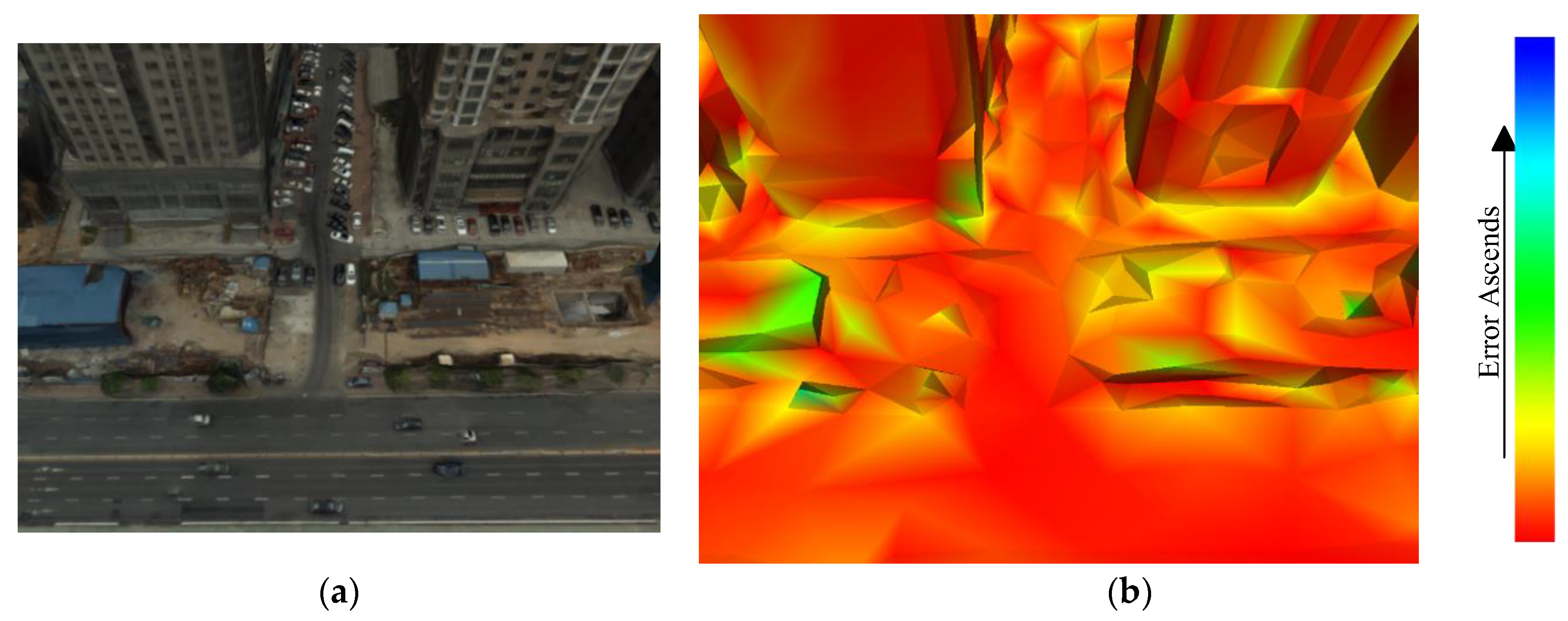
Figure 3.
Two intervals with values of approximately zero appear. The first is located at the start, indicating that an entirely planar surface does exist. The interval between the two quasi-zero intervals represents a planar surface. Therefore, is located in the second quasi-zero interval.
Figure 3.
Two intervals with values of approximately zero appear. The first is located at the start, indicating that an entirely planar surface does exist. The interval between the two quasi-zero intervals represents a planar surface. Therefore, is located in the second quasi-zero interval.
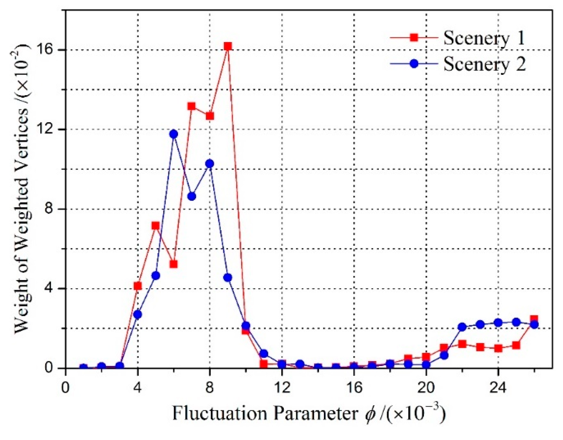
Figure 4.
As expected, that corresponds to the minimum is located in the second quasi-zero interval in Figure 3. This dual mechanism used to find is conducive to identifying the outlier of the judgment that is not located in the second quasi-zero interval. (a) Scenery 1; (b) Scenery 2.
Figure 4.
As expected, that corresponds to the minimum is located in the second quasi-zero interval in Figure 3. This dual mechanism used to find is conducive to identifying the outlier of the judgment that is not located in the second quasi-zero interval. (a) Scenery 1; (b) Scenery 2.

Figure 5.
In most cases, the threshold of the fluctuation parameter decreases as the simplification rate increases or the level of LOD decreases, initially indicating higher planarity of planar surfaces after the simplification of urban surfaces. (a) Scenery 1; (b) Scenery 2.
Figure 5.
In most cases, the threshold of the fluctuation parameter decreases as the simplification rate increases or the level of LOD decreases, initially indicating higher planarity of planar surfaces after the simplification of urban surfaces. (a) Scenery 1; (b) Scenery 2.

Figure 6.
Different methods for detecting planar surfaces (in red). (a) Input 3D model with texture. (b) Recognition of planar surfaces according to the dihedral angles of edges. (c) The planarity of vertices without extension based on the threshold of dihedral angle. (d) The planarity of vertices with extension (our method). It is apparent that (d) better matches the continuity of the playground.

Figure 7.
Planar face extraction compared with simplified ones at level 6 (simplification rate: 0.784) by DVDC (). Recognition of planar surfaces on the basis of (a) recognition of planar vertices with extension and (b) the dihedral angles of edges. It is evident that (b) better matches the continuity of the playground.

Figure 8.
The number of consecutive surface clusters using the extraction of planar surface extraction compared with simplified surfaces using dihedral angles of edges as rulers. It is seen that different simplification algorithms and different input surfaces influence the appropriate simplification rate that can use dihedral angles as rulers. For example, it is suitable for scenery 2 below level 4 with aQSlim as the simplification algorithm. (a) Scenery 1; (b) Scenery 2.
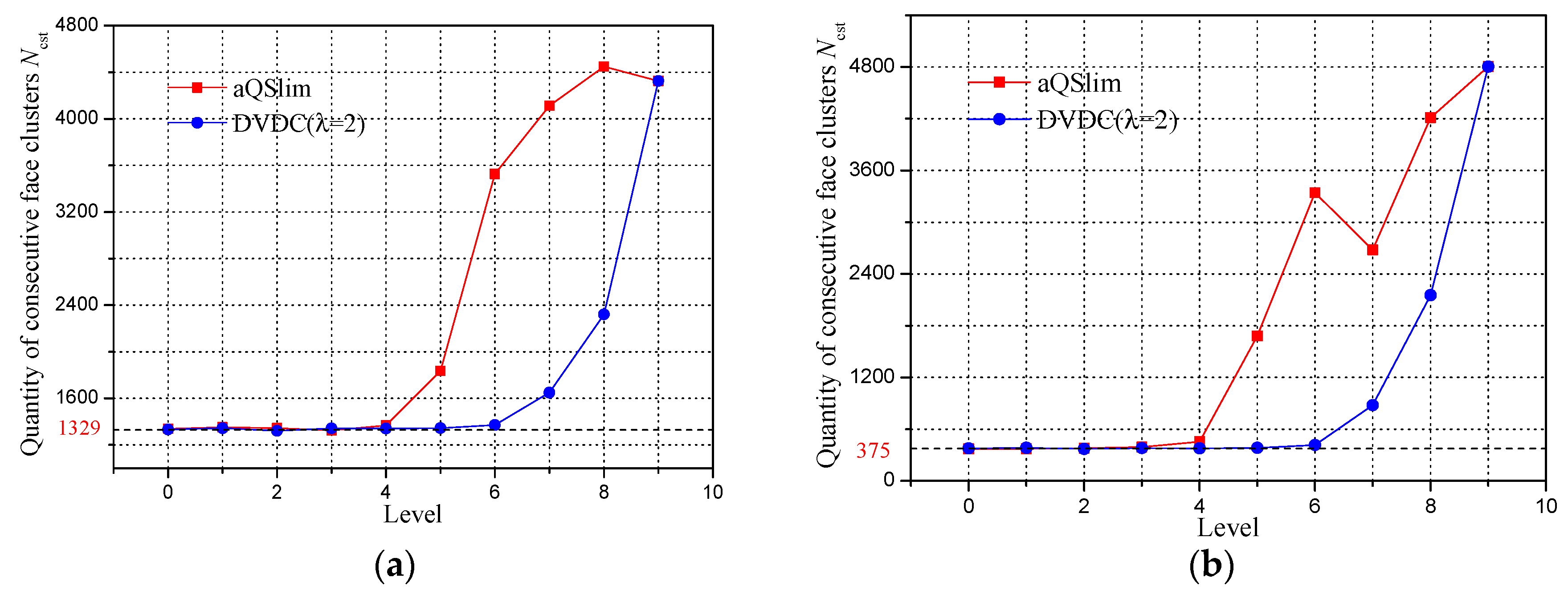
Figure 9.
When the LOD level is not larger than 4, the proportion of virtual faces is stable and close to the largest values, as expected. Emphasis on virtual faces is described for the stage of sampling in Section 4.
Figure 9.
When the LOD level is not larger than 4, the proportion of virtual faces is stable and close to the largest values, as expected. Emphasis on virtual faces is described for the stage of sampling in Section 4.

Figure 10.
(a) Input surfaces with texture; (b) sub-planar edges (red borders) extracted with 0.9 simplification by QSlim. Sub-planar edges are approximately consistent with our subjected image of urban infrastructure.
Figure 10.
(a) Input surfaces with texture; (b) sub-planar edges (red borders) extracted with 0.9 simplification by QSlim. Sub-planar edges are approximately consistent with our subjected image of urban infrastructure.

Figure 11.
Every line in this figure is a median of triangular faces. When the perimeter of a triangle exceeds double, use the next sampling method. The lengths of the edges in this illustration are red > green > blue. Triangle (3) is set as standardized sampling, which is the average perimeter of all faces on surfaces, and triangle (4) represents a rearrangement of a triangular face into six individuals.

Figure 12.
Comprehensive mean error measured by Metro. QSlim and aQSlim appear to perform much better than the other two simplification algorithms. The difference between QSlim and aQSlim fails to be represented in terms of comprehensive error. (a) Scenery 1; (b) Scenery 2.
Figure 12.
Comprehensive mean error measured by Metro. QSlim and aQSlim appear to perform much better than the other two simplification algorithms. The difference between QSlim and aQSlim fails to be represented in terms of comprehensive error. (a) Scenery 1; (b) Scenery 2.

Figure 13.
Mean error of detailed and planar surfaces. aQSlim clearly performs much better in terms of the mean error of detailed surfaces because aQSlim involves projecting the area into the QEM, which enhances the simplification rate for planar surfaces in urban surfaces. As expected, aQSlim performs worse in terms of the mean error of planar surfaces. ACVD and DVDC () still perform worse in terms of both aspects because of the much higher comprehensive error. (a) Scenery 1; (b) Scenery 2.
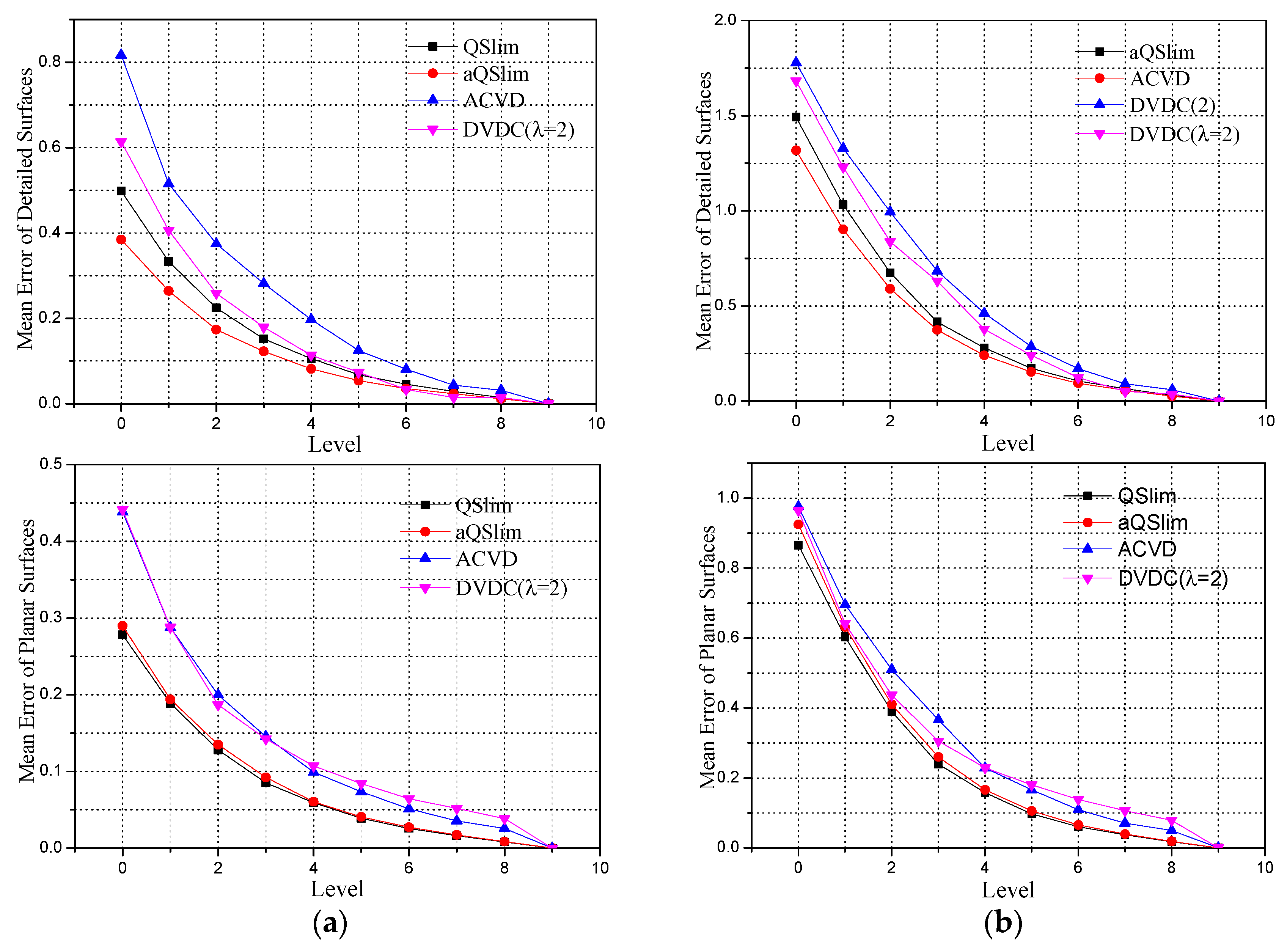
Figure 14.
As expected, aQSlim also performs better than QSlim in terms of the planarity of planar surfaces. However, DVDC () unexpectedly makes planar surfaces more planar, even when the simplification rate is low (the level of LOD is high). (a) Scenery 1; (b) Scenery 2.
Figure 14.
As expected, aQSlim also performs better than QSlim in terms of the planarity of planar surfaces. However, DVDC () unexpectedly makes planar surfaces more planar, even when the simplification rate is low (the level of LOD is high). (a) Scenery 1; (b) Scenery 2.

Figure 15.
Experiments on the proportion of faces of detailed surfaces and the error disparity of detailed surfaces . It is clear that DVDC () performs well in terms of and . It can also be concluded that aQSlim and QSlim perform stably in terms of . (a) Scenery 1; (b) Scenery 2.
Figure 15.
Experiments on the proportion of faces of detailed surfaces and the error disparity of detailed surfaces . It is clear that DVDC () performs well in terms of and . It can also be concluded that aQSlim and QSlim perform stably in terms of . (a) Scenery 1; (b) Scenery 2.
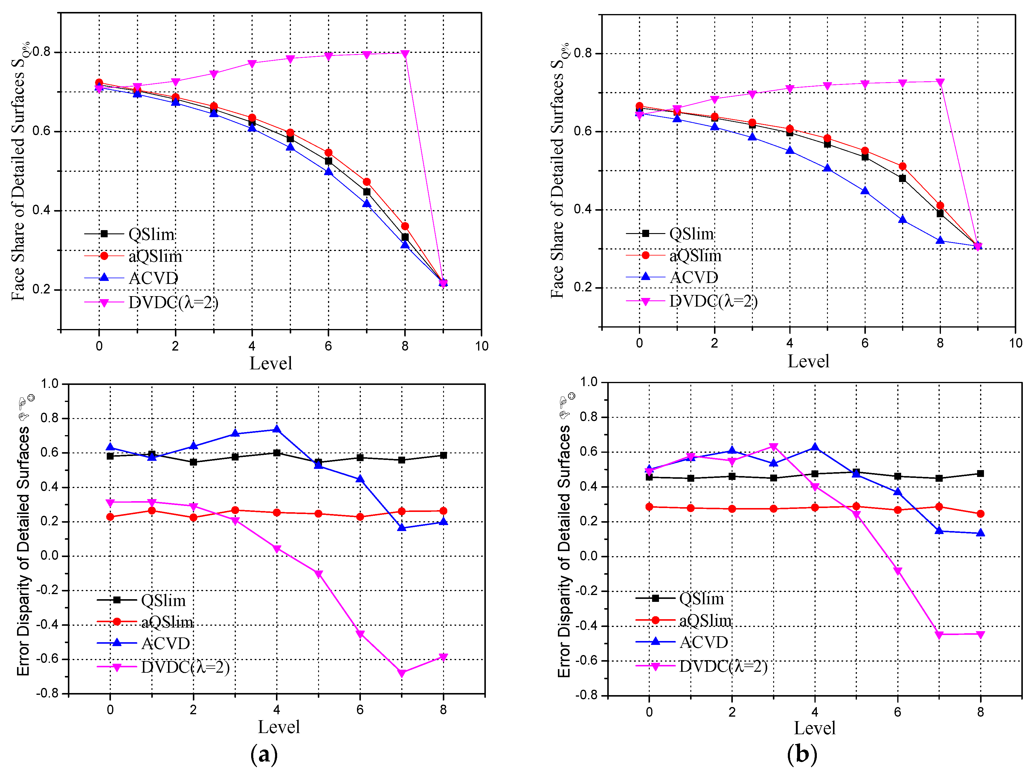
Figure 16.
Error measurement and comparison of the modified simplification algorithm. Given the weakness of Metro pointed out above, the mean errors of all surfaces and detailed surfaces are not consistent. A better property in terms of the error of detailed surfaces proves that mDVDC () better preserves details, which is the core target of surface simplification. (a) Scenery 1; (b) Scenery 2.


Table 1.
Optimal choice of curvature indicator of mDVDC for tile A.
| Mean Error of | Level | ||||
|---|---|---|---|---|---|
| Detailed Surfaces | 4 | 2.2 | 2.3 | 0.027 | 0.088 |
| 3 | 2.3 | 2.4 | 0.015 | 0.093 | |
| 2 | 2.4 | 2.3 | 0.011 | 0.094 | |
| 1 | 2.3 | 2.4 | 0.012 | 0.101 | |
| 0 | 2.3 | 2.4 | 0.017 | 0.082 | |
| Urban Frameworks | 4 | 2.3 | 2.2 | 0.018 | 0.073 |
| 3 | 2.2 | 2.3 | 0.011 | 0.101 | |
| 2 | 2.3 | 2.2 | 0.013 | 0.081 | |
| 1 | 2.3 | 2.4 | 0.012 | 0.078 | |
| 0 | 2.3 | 2.4 | 0.014 | 0.075 |
Table 2.
Optimal choice of curvature indicator of mDVDC for tile B.
| Mean Error of | Level | ||||
|---|---|---|---|---|---|
| Detailed Surfaces | 4 | 1.9 | 1.7 | 0.014 | 0.164 |
| 3 | 2.0 | 1.8 | 0.013 | 0.137 | |
| 2 | 1.7 | 1.8 | 0.016 | 0.147 | |
| 1 | 1.8 | 2.0 | 0.020 | 0.187 | |
| 0 | 1.7 | 1.8 | 0.012 | 0.186 | |
| Urban Frameworks | 4 | 1.8 | 1.7 | 0.017 | 0.142 |
| 3 | 1.8 | 1.9 | 0.015 | 0.161 | |
| 2 | 1.7 | 1.8 | 0.013 | 0.139 | |
| 1 | 1.9 | 1.8 | 0.018 | 0.118 | |
| 0 | 1.8 | 1.9 | 0.016 | 0.158 |
Table 3.
Comparison of time performance between Metro and our methods. From the Table, the time performance is close to and even better than that of Metro.
Table 3.
Comparison of time performance between Metro and our methods. From the Table, the time performance is close to and even better than that of Metro.
| Surface | Face No | Metro (/s) | Without Framework Measurement (/s) | With Framework Measurement (/s) |
|---|---|---|---|---|
| Scenery 1 | 3145277 | 167.26 | 149.17 | 173.14 |
| Scenery 2 | 2392672 | 141.51 | 127.99 | 145.63 |
| Tile A | 109936 | 7.2891 | 10.318 | 12.346 |
| Tile B | 160834 | 9.8672 | 13.911 | 14.713 |
© 2019 by the authors. Licensee MDPI, Basel, Switzerland. This article is an open access article distributed under the terms and conditions of the Creative Commons Attribution (CC BY) license (http://creativecommons.org/licenses/by/4.0/).
Share and Cite
MDPI and ACS Style
Liu, S.; Yi, H.; Chen, X.; Wang, D.; Jin, W. Multifaceted Geometric Assessment towards Simplified Urban Surfaces Built by 3D Reconstruction. ISPRS Int. J. Geo-Inf. 2019, 8, 360. https://doi.org/10.3390/ijgi8080360
AMA Style
Liu S, Yi H, Chen X, Wang D, Jin W. Multifaceted Geometric Assessment towards Simplified Urban Surfaces Built by 3D Reconstruction. ISPRS International Journal of Geo-Information. 2019; 8(8):360. https://doi.org/10.3390/ijgi8080360
Chicago/Turabian StyleLiu, Sheng’en, Hui Yi, Xiangning Chen, Decheng Wang, and Wei Jin. 2019. "Multifaceted Geometric Assessment towards Simplified Urban Surfaces Built by 3D Reconstruction" ISPRS International Journal of Geo-Information 8, no. 8: 360. https://doi.org/10.3390/ijgi8080360
Note that from the first issue of 2016, this journal uses article numbers instead of page numbers. See further details here.