Modeling Words for Qualitative Distance Based on Interval Type-2 Fuzzy Sets


1
School of Geographic and Environmental Sciences, Tianjin Key Laboratory of Water Resources and Environment, Tianjin Normal University, Tianjin 300387, China
2
Institute of Remote Sensing and GIS, Peking University, Beijing 100871, China
*
Author to whom correspondence should be addressed.
ISPRS Int. J. Geo-Inf. 2018, 7(8), 291; https://doi.org/10.3390/ijgi7080291
Submission received: 22 May 2018
/
Revised: 10 June 2018
/
Accepted: 20 July 2018
/
Published: 24 July 2018
Abstract
:Modeling qualitative distance words is important for natural language understanding, scene reconstruction and many decision support systems (DSSs) based on a geographic information system (GIS). However, it is difficult to establish the relationship between qualitative distance words and quantitative distance for special applications since the meanings of these words are influenced by both subjective and objective factors. Some existing methods are reviewed, and the Hao–Mendel approach (HMA) is improved to model qualitative distance words for four travel modes by using interval type-2 fuzzy sets (IT2 FSs), aiming at addressing the individual and interpersonal uncertainty among qualitative distance words. The area of the footprint of uncertainty (FOU), fuzziness (entropy), and variance are adopted to measure the uncertainties of qualitative distance words. The experimental results show that the improved HMA algorithm is better than the original HMA algorithm and can be used in spatial information retrieval and GIS-based DSSs.
1. Introduction
Spatial relations are important for geographical information systems (GISs), artificial intelligence (AI), decision support systems (DSSs) and image analysis [1,2,3,4,5]; and they are usually classified as topological relations, directional relations, and distance relations which are further divided into quantitative and qualitative distance relations. The qualitative distance relations describe the proximity between spatial objects using natural language [6], such as “The Tianjin Binhai International Airport is far away from the Tianjin Railway Station” and “Many hotels are near the Tianjin Railway Station”. In these statements, “far” and “near” are vague words that describe qualitative distance relations. From a linguistic point of view, a large number of linguistic distance concepts are available to qualitatively describe distance [7,8]. In some knowledge-based geospatial analysis and mining systems, the number of the required qualitative distance words depends on the level of granularity; e.g., using “far” and “near” at a rough level and “very close”, “close”, “medium”, “far”, and “very far” at a relatively fine level. In addition, another key issue is to determine the semantics of each qualitative distance variable, which is important for natural language understanding, scene reconstruction and many GIS-based DSSs [2,3]. Although natural language is gradually becoming an important data source for GISs [9] and some studies interpreted fuzzy semantics of natural language spatial relation (NLSR) terms using the fuzzy random forest (FRF) algorithm and fuzzy sets [5,10], most GISs currently cannot handle natural language effectively, and most linguistic descriptions about spatial relations cannot be used in current GISs. This issue has not yet been solved; therefore, how to integrate the spatial relationships described in natural language into a GIS is a challenge in the field of GIS [11]. The relationship between qualitative distance words in natural languages and quantitative distance must be established [12].
In the past 20 years, many scholars have performed much work to study the connotation of qualitative distance words, including “near”, “close to”, “adjacent”, and “surrounding” [13,14,15]. Different methods are used to establish the relationships between qualitative distance words and quantitative distance, and to build context-contingent translation mechanisms and computational models between linguistic proximity descriptors and metric distance measures [16]. However, establishing such a relationship is a very difficult task because it is influenced by many factors, such as the application scene (environment), context, psychological and physiological characteristics of the subject, culture, travel destination and travel mode [6,11,13,15,16,17]. From the psychometric testing of perceived proximity, Gahegan noted that the definition of proximity is related to five aspects [13]. Clementini et al. emphasized that the concept of proximity is context dependent [6]. Yao and Thill classified the context factors of proximity perception into objective and subjective factors [11]. Overall, the factors that affect the connotation of qualitative distance are very complex.
Due to the ambiguity of qualitative distance words, many people adopt fuzzy sets to establish the relationships between qualitative distance words and quantitative distance, and these methods generally fall into three types. The first type establishes the distance membership functions directly for the decision system based on the experience of experts [18]. In actual operation, the parameters of the distance membership functions should be adjusted according to the effect of the decision systems; thus, this type of method is very subjective. The second type establishes the connotation expression of the qualitative distances by mining Web text resources related to the qualitative distance descriptions [14,19]. The advantage of this approach is that the resources of the sampling are very rich, but it is difficult to define valid membership functions because different application scenarios may require different definitions. Another issue is that guaranteeing the authenticity and objectivity of Web text is difficult. For example, when real estate agents are advertising houses, the location of the house relative to other locations of importance can be falsified to promote sales. Therefore, even if a supermarket or school is four kilometers away from a house, the agents may say that the supermarket or the school is near the house. The third type investigates a specific population using questionnaires and obtains knowledge regarding their qualitative distances; a mapping relationship between qualitative distance words and quantitative distance is then established by means of statistics and regression [11,16,20,21,22]. Compared to the methods mentioned earlier, the methods of this type allow for the dynamic construction of context-contingent proximity models based on sample data. These methods are more suitable for GIS-based DSSs, as these systems are often oriented toward a particular population and a specific task. One problem that exists in the method of Yao and Thill [11,16] is that it is difficult to quantify these factors because many factors themselves are vague. At the same time, how these factors affect the meaning of qualitative distance words, which may involve the mechanism of cognition, is difficult to determine.
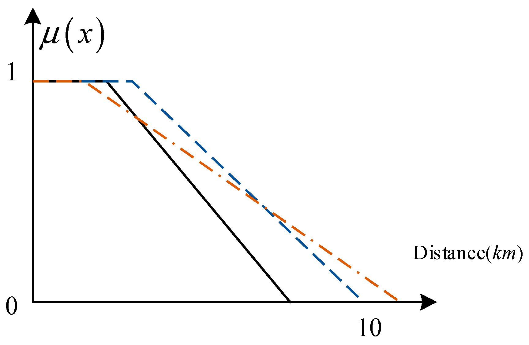
From the perspective of the semantic meaning of spatial vocabulary, the semantics of words that describe the spatial locations and spatial relationships of crisp or fuzzy objects are typically uncertain. Usually, a linguistic distance measure implies a different spatial range for different people. Figure 1 shows three classical fuzzy sets (i.e., type-1 fuzzy sets, T1 FSs) for the distance word “near” perceived by three people, indicating that the same words may have different meanings for different people in the real world. Moreover, there is some semantic uncertainty between these T1 FS models, i.e., interpersonal uncertainty of words [23,24]. Mendel [25] introduced six principles associated with evaluation methods used to obtain FS models for a word in computing with words (CWW). The T1 FS models of words violate principle three: “Words contain linguistic uncertainties, i.e., words mean different things to different people, and so the FS model that is used to represent a word must be able to incorporate both of these uncertainties”. The T1 FS has no ability to handle this kind of semantic uncertainty because the membership degree of a T1 FS is a single value.
The main goal of this study is oriented towards CWW; that is, the direct use of natural language words as objects of computation, based on interval type-2 fuzzy set (IT2 FS), is adopted to model qualitative distance words, and then the semantic uncertainty of distance words can be addressed. The Hao–Mendel approach (HMA) [25,26] is an effective means to estimate the fuzzy set after collecting data related to the words because it is the only method to-date that leads to normal interval type-2 fuzzy sets. However, HMA considers only the uncertainty of the upper membership function of an IT2 FS, not the entire uncertainty of the IT2 FS. To address this, the HMA algorithm is first improved by the entire uncertainty of IT2 FS, called the improved HMA, and then the IT2 FSs for distance words are established by the improved HMA in this study. The remainder of this article is organized as follows. In the second section, some basic concepts related to this article are introduced, such as IT2 FS and CWW. In the third section, the HMA algorithm is improved for distance words. In the fourth section, an experiment is conducted to verify the improved HMA algorithm and then the improved HMA algorithm is compared with the original HMA algorithm using three uncertainty indices. The results show that the improved HMA algorithm is better than the original algorithm. The characteristics of the qualitative distance models established using the improved HMA algorithm are then analyzed based on these three indices. Conclusions are presented in the fifth section. Appendix A is the questionnaire and all Abbreviations and their definitions used in this paper are listed in Appendix B.
2. Background
In this study, IT2 FSs are used to model distance words. This section introduces concepts such as CWW and IT2 FS. In addition, several uncertain indices related to qualitative distance words are introduced.
2.1. CWW
CWW is a methodology in which the objects of computation are words and prepositions drawn from a natural language. CWW was first introduced by Zadeh [27,28] and has been widely used in market investments, decision-making analyses, automatic control designs, fuzzy queries, data mining, and other fields. According to the existing literature, CWW techniques fall into three categories: membership-function-based models, symbolic linguistic computing models and 2-tuple linguistic models. Each category of models is unique in its advantages and limitations [29,30,31]. Li et al. proposed a new CWW framework based on the 2-tuple linguistic model [32]. Such a CWW framework allows people to address personalized individual semantics (PIS) to allow CWW to maintain the idea that words mean different things to different people.
2.2. IT2 FS
The T1 FS theories have been applied to many domains because of their ability to model fuzziness. However, the membership degree of a T1 FS is a single value, so T1 FS cannot manage the errors associated with the membership values of fuzzy objects, as shown in Figure 2a. Zadeh introduced the type-2 fuzzy sets and type-N fuzzy sets to overcome this flaw of T1 FS [28]. The primary membership function of a common type-2 fuzzy set (T2 FS) is a type-1 fuzzy set, which makes computation extremely difficult. Thus, the application of the T2 FS to a real task is comparatively difficult.
The IT2 FS is a special case of T2 FS and it uses an interval to express the primary membership value (Figure 2b). The IT2 FS is better than the T2 FS in complexity and computation, so it is adopted in this study. Many authors refer to interval type-2 fuzzy sets as type-2 fuzzy sets and add the qualifying term ‘generalized’ only when discussing non-interval type-2 fuzzy sets [33,34]. Fuzzifying the spatial data that contain certain types of errors is necessary and can achieve error containment. For example, geological, topographical and environmental parameters are required to assess regional debris flow hazards, and some parameters have vague boundaries. Therefore, the IT2 FS is a more reasonable choice to solve fuzzy geographical problems. The interval-valued fuzzy set (IVFS) is a special case of the IT2 FSs [35]. In this paper, the definition of IT2 FS introduced by Mendel is adopted.
Definition 1.
(Interval type-2 fuzzy set) [26]: an IT2-FSin the universeis given by:
whereis the universe of discourse for the secondary variable. Note thatis a subset of [0, 1].
For the sake of convenience, the IT2 FS is represented as , and and are the lower membership function (LMF) and upper membership function (UMF), respectively. The footprint of uncertainty (FOU) of an IT2 FS is the uncertainty in the primary memberships , and it has always had the connotation of a geometric object bounded by a UMF and an LMF, as shown in Figure 2b.
The interval type-2 fuzzy set is adopted to model qualitative distance words as shown in Figure 2c. It is a normal, trapezoid interval type-2 fuzzy number that can be expressed as:
where and are the LMF and UMF, respectively. They can be expressed as:
and
2.3. IT2 FS Uncertainty Measures
Three uncertainty indices of IT2 FSs are used in this study to measure the uncertainties of IT2 FS models corresponding to qualitative distance words: area of the FOU, fuzziness (entropy) and variance [36]. The fuzziness (entropy) is an uncertainty measure of the membership domain, and variance is an uncertainty measure of the Euclidean space domain.
2.3.1. Fuzziness (Entropy) of an IT2 FS
The fuzziness (entropy) of an FS can quantify the amount of ambiguity of a fuzzy set. Many definitions of fuzziness for IT2 FSs have been proposed [36,37,38].
Definition 2.
Definition 3.
The fuzziness of an IT2 FSproposed by Wu and Mendel [36], denoted by, is the union of all cardinalities of its embedded T1 FSs, i.e.,:
where,, and. To computeand, letbe defined as:
and letbe defined as:
Then,, and.
2.3.2. Variance of an IT2 FS
The variance in a T1 FS measures its compactness; i.e., a smaller (larger) variance means that is more (less) compact.
Definition 4.
The varianceof an IT2 FSis the union of relative variance of all its embedded T1 FSs; i.e.,:
whereis the relative variance of an embedded T1 FSrelative to the IT2 FS, andis the average centroid of, which can be calculated using the KM algorithms [39,40].are the minimum and maximum relative variances of all, respectively.
3. Modeling Qualitative Distance Words
The HMA algorithm is used to model adverbs as IT2 FSs in the interval [0, 10], such as “very little” and “moderately”. It is composed of two parts: data processing and fuzzy sets. As discussed before, the semantic connotation of distance words may be affected by the travel mode; that is, different travel modes may have different spatial ranges. For example, generally, we estimate that the spatial range of the walking distance of ordinary human subjects is [0, 3] km, and the spatial range of the cycling distance is [0, 10] km. A spatial distance larger than 20 km may be very far for the two travel modes. The upper limit of “very far” is uncertain and can even be infinitely large. Therefore, the HMA algorithm is not suitable for modeling qualitative distance. In addition, the HMA algorithm calculates the parameters of an IT2 FS by using only the standard deviation intervals and the standard deviation of the UMF of the IT2 FS, but ignores the standard deviation of the LMF of the IT2 FS. In other words, this algorithm does not consider the entire uncertainty of the IT2 FS. As a result, the HMA algorithm must be improved to model qualitative distance. For the sake of discussion, the qualitative distance linguistic variable consists of five words in this study, i.e., “very near (Vnear)”, “near”, “medium”, “far”, and “very far (Vfar)”. The membership functions of each word can be determined using the improved HMA algorithm.
3.1. Collecting Data
Four travel modes are considered in this study: walk, bicycle, public transportation and train. The first three are interurban travel modes, whereas the fourth is a travel mode between cities. Via questionnaires, the distance interval sets corresponding to the five qualitative distance words for each travel mode are obtained. As mentioned in Section 1, the factors affecting the qualitative distance relationships are very sophisticated, and the impact of each factor is impossible to quantify. Therefore, the data uncertainty should be reduced by the following assumptions: (1) The scope of the survey is limited to grade 3 and 4 university students, as most of them are aged 21 to 23 years old and are familiar with the city environment; (2) the geographical environment is normal; i.e., mountains, deserts or other special environments are not considered; (3) the physical condition of each respondent is normal, and the weather is also normal. Some special physical conditions are not considered, including illnesses and hunger or special weather conditions such as snow, low temperatures and strong winds; (4) For the four travel modes, the lower limit is 0, and the upper limits are 5 km, 10 km, 30 km and 2000 km, respectively; (5) the intervals obtained from one person for the five words cannot overlap, and there is no gap between them; (6) a normal goal is set for each travel mode, as urgent tasks affect our perception of distance. The questionnaire used in this study is attached in Appendix A.
3.2. The Improved HMA Algorithm
As discussed previously, the original HMA algorithm does not consider the entire uncertainty of the IT2 FS; in this section it is improved by the entire uncertainty of the IT2 FS, and called the improved HMA. This improved HMA is still based on the questionnaire, and five interval sets corresponding to the five distance words for each travel mode are obtained. For the j-th word, the i-th subject provides interval endpoints and , and the group of n subjects provides . In this study, the variables are normalized by the upper limit value to l = 0 and r = 10.
3.2.1. Data Processing
During data processing, statistics and probability are used to handle these interval sets and to reduce model uncertainty corresponding to distance words. This part involves five steps:
- (1)
- Correcting and removing bad data. As not everyone takes a survey seriously, some bad data may seriously pollute the interval sets and affect the statistics. To ensure the correctness of the statistical results, the intervals of the i-th subject should be removed if one of the following four conditions is true: (1) The data intervals of the i-th subject overlap with each other; (2) there is some gap between these intervals; (3) the value of the interval that corresponds to “very far” is greater than the threshold; (4) all intervals of the i-th subject are much larger or smaller than others. If the value of the interval corresponding to “very far” is greater than the threshold (different thresholds for four travel modes are set in Section 3.1), then should be set as the threshold. If the value of the interval corresponding to “very near” is greater than 0, then should be set to 0. subject intervals will remain.
- (2)
- Normalizing the data. As mentioned previously, the thresholds for the four travel modes are different. For the sake of convenience, these data should be normalized into a unified range. All subject intervals are normalized into the same range using the threshold value, and l = 0 and r = 10 are set.
- (3)
- Performing outlier processing. To remove some of the noise in the data set, outlier processing is necessary. In this section, the box and whisker tests [41] are performed for the remaining intervals, i.e., only the intervals satisfying Equation (10) are keptwhere (, ) and (, ) are the quartile and interquartile ranges for the left (right) endpoints and the interval length, with .
After outlier processing, data intervals will remain for which the following data statistics will then be computed: , , , , , (mean and standard deviation of the left endpoints, right endpoints and the lengths of these intervals).
- (4)
- Performing tolerance limit processing on the remainingintervals simultaneously. The goal of this stage is to guarantee that the data intervals fall within an acceptable two-sided tolerance limit. Only intervals satisfying Equation (11) are kept.where is the tolerance factor (refer to Reference [32] for detailed information). After tolerance limit processing, data intervals will remain, and the data statistics , , , , , will then be recomputed.
- (5)
- Performing reasonable interval processing. The goal of this stage is to remove data intervals that do not overlap or overlap only slightly with other data intervals. First, the point that best separates the left and the right endpoints set must be found.where . Then, only intervals satisfying Equation (13) are kept. This step reduces the interval endpoints to interval endpoints. The data statistics , , , are then recomputed.
Therefore, the original n data intervals are reduced to a set of m data intervals via this data pre-processing.
3.2.2. Establishing IT2 FSs for Distance Words
As mentioned previously, the original HMA uses the upper membership function to estimate the IT2 FS parameters of words; that is, the standard deviation of a sample is equal to the standard deviation of the UMF in the original HMA, but it does not consider the LMF uncertainty. Consequently, this measurement is unilateral, and the uncertainties of these IT2 FSs may be exaggerated. As we know, the FOU of an IT2 FS is constructed by the LMF and UMF, and it is a description of the overall uncertainty of an IT2 FS. The uncertainties of an IT2 FSs may not be exaggerated if the FOU is considered for estimating its parameters. Therefore, in this study, the entire uncertainty (the FOU area) is adopted to estimate the parameters of IT2 FSs of words. First, the type of FOU of each word must be determined. Next, the overlap interval in () must be found. Then, the parameters of the IT2 FS should be determined. The improved HMA consists of the following four steps:
- (1)
- Determining the type of FOU of each word. Three kinds of FOU exist: left-shoulder, right-shoulder and interior FOU, as shown in Figure 3. For an interval set , the one-sided tolerance intervals are computed first, namely, and . , , and are calculated in the last step of the data processing step, and is a one-sided tolerance. Detailed information can be found in Reference [42]. Next, the types of FOU that correspond to each word can be classified as follows:
- (2)
- Determining the overlap interval of the interval set .
- (3)
- (4)
- Determining the parameters of the IT2 FS. As shown in Figure 4, the unknown parameters for the left-shoulder FOU (or right-shoulder FOU) are and ( and ). For the interior FOU, four unknown parameters exist: , , and . The set is used to determine and and is used to determine and .
Let be a right-shoulder FOU or the left-hand portion of an interior FOU. The corresponding small interval set is . The mean length of the interval set is . The mean and the sample standard deviation of the set are and , respectively.
The centroid of , and the average centroid, , are induced by the mean of T1 embedded set of (more information refers to the “Appendix A” of literature [14]) and expressed as:
In Reference [14], the standard deviation of the UMF is used to calculate unknown parameters. Obviously, this value cannot represent the uncertainty of the FOU, while the area of the FOU can reflect the global uncertainty of the membership degree of this FOU. Thus, the area of the FOU is adopted here and is computed as:
Then, and can be calculated as:
such that
The operation prevents and from being negative. Similarly, and can be calculated as:
where and are the mean and sample standard deviation of a left-shoulder FOU or the right-hand portion of an interior FOU, respectively, and .
Thus, the IT2 FS that corresponds to the qualitative distance word can be expressed as:
4. Experimental Results and Analysis
A questionnaire survey was conducted at the School of Geographic and Environmental Sciences, Tianjin Normal University in October 2017. The subjects of this questionnaire survey are grade 3 and 4 university students, and the hometown of most of these subjects is Tianjin City, so they are familiar with the city. The language of this questionnaire is Chinese, and the language used in the questionnaire listed in the Appendix A is the second language of these subjects. During the survey, six assumptions or conditions regarding the respondents were stressed and 86 valid questionnaires were collected and analyzed using four Excel forms. Then, based on the improved HMA algorithm, the parameters of IT2 FSs corresponding to the five qualitative distance words for the four travel modes were calculated (Table 1). These IT2 FSs are presented in Figure 4, Figure 5, Figure 6 and Figure 7.
4.1. General Description of the Qualitative Distance Model
The results were independently reviewed by an entirely separate group of 10 adults, and they all agreed that the results were consistent with actual situations. Regarding the IT2 FSs for each travel mode, the membership value is equal to 1 in the interval [, ] ([, ]), and the length of these intervals is . The interval [, ] is the supporting interval, with the length being . These two intervals have direct directives. Using walking distance as an example, the membership function of the IT2 FS that corresponds to “medium” takes the value of 1 for the distance interval [0.70, 0.80] km, indicating that when most people consider a distance within this interval, they estimate that it is suitable for walking. The interval [1.50, 1.60] km can be estimated to belong to the range of “far”, for which people are likely to choose other transportation modes. When the distance is longer than 3 km, the corresponding range is “very far”; at these distances, people generally forego walking and choose other travel modes. For cycling, the distance interval [2.00, 2.20] km is certainly suitable, but when the distance is approximately [3.50, 4.00] km, people may hesitate to ride a bicycle. In general, when the distance is greater than 6 km, people choose public transportation, such as buses, subways and taxis.
For travel between cities, the distance interval [120, 150] km is estimated to correspond to “near”, as more than 20 thousand km of high-speed railways have been built in China, covering almost all the major cities in China. The speed of these railway trains is approximately 300 km/h; thus, people often say that Beijing is close to Tianjin. When the distance is greater than 1000 km, people may hesitate to travel along the high-speed railway, as the time spent and cost of traveling by train may be greater than those when traveling by airplane.
Figure 4, Figure 5, Figure 6 and Figure 7 and Table 1 show that the IT2 FSs are asymmetrical. For the four travel modes, and gradually increase as the distance increases from very near to very far, with a more obvious increase in than that in . This result intuitively illustrates that the words “far” and “very far” are more ambiguous than “near” and “very near” for all four travel modes.
4.2. Comparison with HMA
In Euclidean space, the domain of quantitative distance is a semi-closed set, i.e., . Thus, it is difficult to determine the upper limit of “Vfar” in real applications, and different upper limits of “Vfar” can yield different IT2 FSs, which may lead to different measures of uncertainty. Consider the train travel mode as an example. If its upper limit is less than 1800 km, the FOU, cardinality, fuzziness and variance of the IT2 FSs may be different for different upper limits. If its upper limit is larger than 1800 km, the FOUs of different IT2 FSs, which are modeled using different upper limits, are equal; in contrast, their cardinality and variance are not equal. Notably, the values of the LMF and UMF of the IT2 FSs corresponding to “Vfar” for the four travel models are equal to 1 when the quantitative distance is larger than . Thus, the upper limits of “Vfar”, , should be set for convenience of analysis. Then, the area of the FOU, cardinality, fuzziness, and variance of these IT2 FSs, modeled using the improved HMA and the original HMA, are calculated, as shown in Table 2. The two rows, Fuzziness 1 and Fuzziness 2, are computed based on the definitions in References [36,38] respectively, and the value in the Total column is the sum of the columns Vnear, Near, Medium, Far and Vfar.
As mentioned previously, the FOU is the uncertainty measure of the primary memberships of a T2 FS. Thus, a small FOU area indicates low uncertainty regarding the IT2 FS; in geometric terms, an IT2 FS with a smaller FOU area is thinner than that with a larger FOU area. Table 2 shows that the total area of the FOU of these IT2 FSs modeled by the improved HMA is smaller than that obtained by the original HMA. Moreover, the fuzziness (entropy) and variance of these IT2 FSs modeled by the improved HMA are smaller than those by the original HMA, having a strong correlation with the area of the FOU. Therefore, in terms of uncertainty, the improved HMA is better than the original HMA.
4.3. Compactness and Fuzziness Analysis
As introduced earlier, the quantity variance is an uncertainty measure in the spatial domain. For the four travel modes, from “Vnear” to “Vfar”, the variance increases; for example, the variance of the IT2 FS of “Vnear” is 867, whereas that of “Vfar” is 145,663. The variances of IT2 FSs for traveling by train and walking experience the most significant increases, followed by bicycle travel. Particularly, for bicycle and public transportation, the variance value of the IT2 FS of “Vnear” is larger than that of “near”. This shows that for these four travel modes, people’s cognitive ambiguity regarding “very far” or “far” is larger than that of “near”, whereas for bicycle and train modes, the cognitive ambiguity of “Vnear” is larger than that of “near”. The variation tendency of fuzziness is similar to that of variance, especially for Fuzziness 2. The values of the IT2 FS of “Vfar” in the row of Fuzziness 2 are significantly larger than those of “Vnear”.
In summary, no matter what the travel mode is, the semantic uncertainty of “Vfar” is the greatest, whereas the uncertainty of “near” (“Vnear”) is the smallest. In other words, the spatial scope of “near” is easy for people to agree on, but there is a large difference in the spatial ranges of “far” and “Vfar”.
4.4. Comparison with Other Methods
In Section 4.3 and Section 4.4, we present a full comparison of the improved and original HMAs and show that the improved HMA is better than the original. As discussed in the Introduction, there are three types of methods typically used to establish the relationships between qualitative distance words and quantitative distances. In this section we present a comparison with these methods.
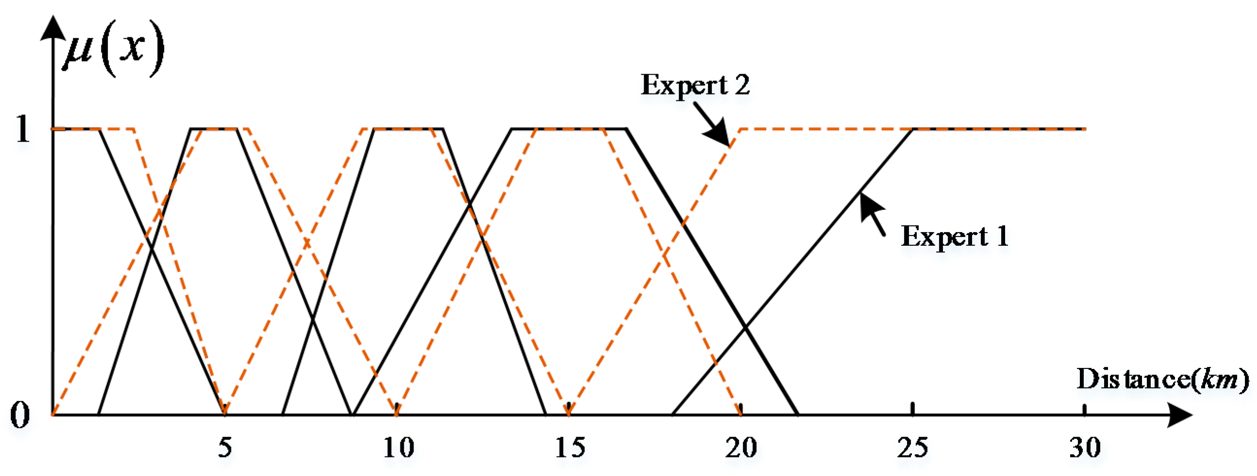
The parameters of the distance membership functions in the first type directly depend on the experience of the experts and are extremely subjective. In addition, a complex decision support application often involves multiple experts, and these experts have different understandings of qualitative distance words. As Yao and Thill [11] noted, a linguistic distance measure, e.g., near, implies different trip distances for different people. Therefore, the fuzzy membership functions of distance words based on their personal cognitive habits are likely to be inconsistent, as shown in Figure 8. In other words, membership functions established by this method do not reflect the semantic uncertainty among experts. The data used in the proposed method are from multiple subjects, and the semantic uncertainty of subjects can be expressed through the upper and lower membership functions, thereby yielding a more objective method. The second type method discussed in section one involves establishing membership functions by collecting data from Web text. The context of a distance word in Web text may be different, and the semantics of qualitative distance words depend on context [11,16,21]. Therefore, it is difficult to establish membership functions of distance words for a specific context or specific task based on this method. Additionally, the membership functions established in this manner are type 1; therefore, they cannot express the semantic uncertainty of words among different people.
The third type methods discussed in section one are used to establish fuzzy sets corresponding to qualitative distance words through questionnaires. In the spatial relation acquisition station (SRAS) [9,28], subjects answer questions as YES or NO based on a map, such as “Is the city of Blackshear close to Douglas?”, then the fuzzy distance relation between geographical features can be derived by fuzzy logic method. While Robinson’s effort is worthwhile in many respects, it does not incorporate the influence of the context of the query on the mapping of proximity spatial relations [11]. But beyond that, it has no ability to establish fuzzy sets for distance words. Yao and Thill [16] highlighted the importance of context and noted that considering the relationship between the context and the metric properties of data is necessary. Additionally, the Adaptive Neurofuzzy Inference System (ANFIS), a Takagi-Sugeno fuzzy inference system, was adopted, and the linguistic proximity measure was predicted based on the metric distance and contextual factors and expressed as based on fuzzy rules. The prediction is affected by the number of factors, types of factors, fuzzification method, and the rules and reasoning of the model. For example, as previously noted, it is difficult to fuzzify these factors, and unsuitable fuzzification methods may introduce new uncertainty. However, the translation from metric distance to linguistic distance in Reference [16] is inexplicit. Grütter et al. [43] claimed that this process does not support the translation of local prepositions, such as “near” or “far”, into distance measures processed in metric systems and that the information required to link the numerous contextual variables may not be available in practical applications. Hence, it is often difficult to implement these processes on large scales. In Yao and Thill’s other method [11], namely the Ordered Logit Regression approach, probability functions of distance words are induced by Ordered Logit Regression; however, the maximum value of the first four functions is less than 1, which is contrary to human cognition, because in general, we can always determine a spatial range and the distance between this range to the reference object is near or far away.
Although many methods abovementioned could be used to establish FS models for distance words, to the best of our knowledge, they are related to T1 FS models and violate principle three introduced in Section 1. Because the membership function of a type-1 FS does not provide flexibility for simultaneously incorporating both types of linguistic uncertainty, it is therefore scientifically incorrect to model a word using a T1 FS [23]. Our method uses an IT2 FS to model distance words, can handle both types of linguistic uncertainty, and is context dependent. Overall, the proposed method is better than the other methods discussed.
4.5. Practical Application
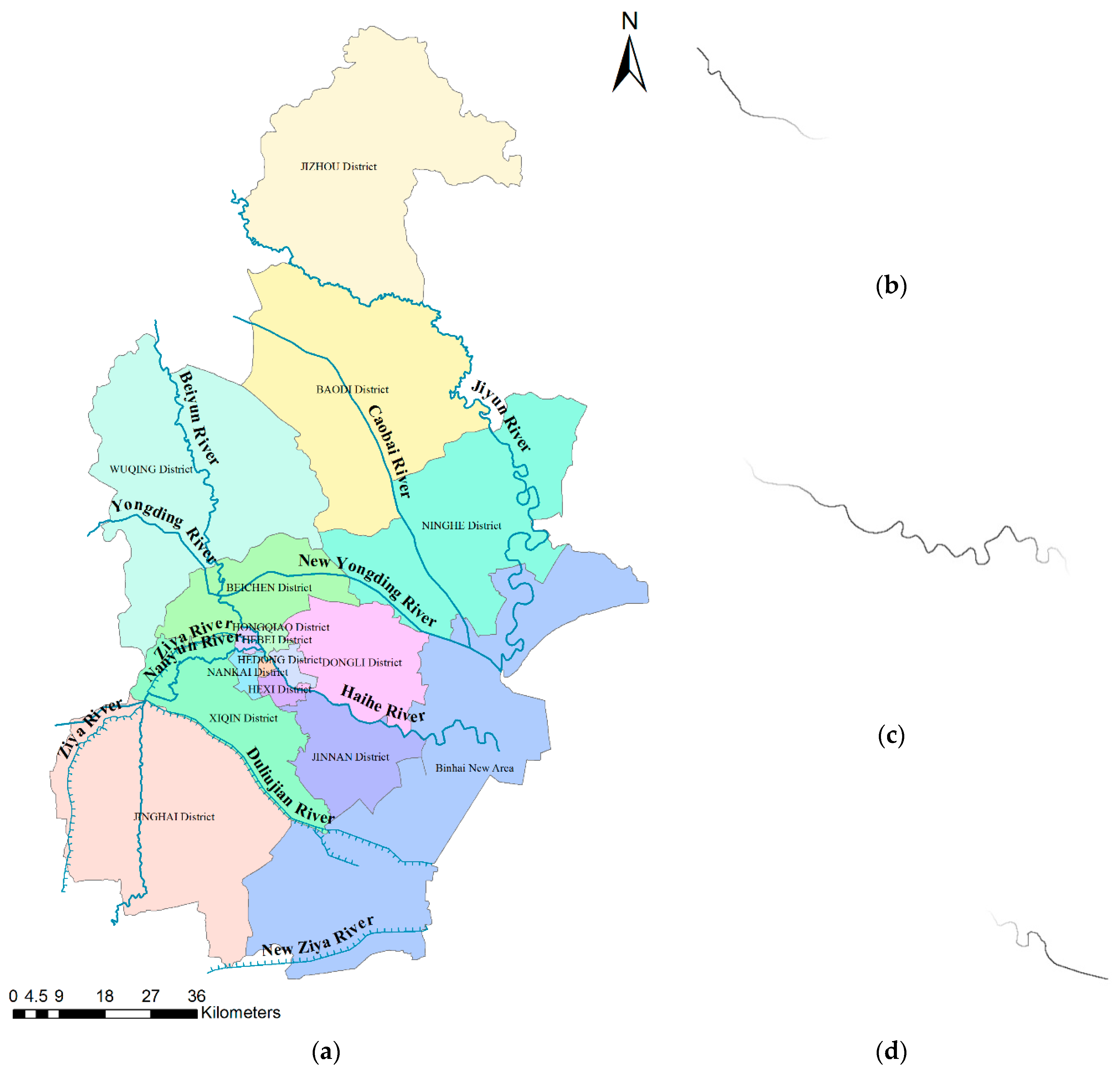
In this section, a case study on natural language spatial queries was used to illustrate the usefulness and effectiveness of our presented methods. The Haihe River is the main river in Tianjin City, and the surrounding area of the upstream part of the Haihe River is the city center. The infrastructure in this region is very mature. There are many famous and desirable primary schools in this region. If a school is too close to the river, children will sneak off to the riverside to play. This is very dangerous for children, so parents tend not to favor such schools. As a result, it is useful to determine which primary school is a medium distance from (not too near) the upstream section of the Haihe River, and the results can provide advice for parents’ guidance to choose primary schools. In Reference [33], we divided the river into upstream, midstream and downstream sections by using the fuzzy partition method as shown in Figure 9.
In Section 4.1, the IT2 FS corresponding to “medium” distance by cycle is . The region with medium distance to the Haihe River by bicycle can be determined by the fuzzy logic method [33], shown in Figure 10a,b. Schools located in the medium distance, which is modeled as IT2 FS to the upstream of the Haihe River, are listed in Table 3, we can see that the membership degree of each school belonging to the “medium” distance to the upstream of Haihe River is an interval value, i.e., the membership grade of “KUN MING LU XIAO XUE” is [0.9568, 0.9767], and error of membership grade is 0.0199. When the upper membership grade decrease from 1 to 0.5, the error of membership grade increases from 0 to 0.4219. It means that when the upper membership grade is near to 0.5, the semantic uncertainty is great. On the contrary, when the distance words are modeled as T1 FS, the membership grade is a singleton and the error of membership grade cannot be measured. So, modeling distance words as IT2 FS is more reasonable and flexible than modeling as T1 FS.
On the other hand, we obtain 71 primary schools in this region by optimistic query when the upper membership grade is greater than 0.5, shown in Figure 10c. and we can obtain 50 primary schools by pessimistic query when the lower membership grade is greater than 0.5, shown in Figure 10d. So, there are 21 difference between the optimistic and pessimistic query. However, when the distance word is modeled as T1 fs, due to it not being able to express the semantic uncertainty, users can only query in one way, and the result of the query is more arbitrary and monotonous than the method proposed in this paper.
5. Conclusions
People use qualitative distance words to describe the approximate positions of objects relative to one another in natural languages. The meanings of qualitative distance words depend on objective factors. If these words are used by people in different contexts, their connotations will be different. Therefore, a unified fuzzy set representation of qualitative distance words is impossible to establish for all GIS-based decision support systems. In other words, the fuzzy set representation of distance words can be obtained for specific tasks. First, aiming at the shortcomings of the original HMA algorithm, the HMA method is improved by introducing the area of the FOU. Then, the improved HMA algorithm is used to establish the IT2 FS representation of qualitative distance words. Three uncertainty indices, i.e., the area of the FOU, fuzziness (entropy), and variance, are used to measure the uncertainties of these IT2 FSs. Experimental results show that the values of these indices for the IT2 FSs obtained by the improved HMA algorithm are smaller than those obtained by the original HMA algorithm. This indicates that the improved HMA algorithm is better than the original algorithm. In addition, it shows that the semantic uncertainty of “Vfar” is the greatest, while that of “very near” (“Vnear”) is the smallest, no matter which travel mode is considered. Hence, the cognitive fuzziness of “far” is larger than that of “near”. In other words, the spatial scope of “near” is easy for people to agree on, but there is a large difference in the spatial range of “far”.
The qualitative distance, topological relationship and direction relationship are often used together to describe a spatial position in natural languages. Therefore, in a follow-up study, the IT2 FS representation of the qualitative distance established in this study will be used to study the semantic spatial relationship by being combined with topological and direction relationships.
Author Contributions
J.G. conceived and designed the research, implemented the improved HMA algorithm in Java and wrote the manuscript. S.D. analyzed results and revised the manuscript.
Funding
This work was supported by the Chinese National Nature Science Foundation (No. 41101352), the Key Project of the Tianjin Natural Science Foundation of China (17JCZDJC39700) and the Innovation Team Training Plan of the Tianjin Education Committee (TD13-5073).
Acknowledgments
The authors wish to thank the anonymous reviewers who provided helpful comments on earlier drafts of the manuscript.
Conflicts of Interest
The authors declare that they have no conflicts of interest to disclose.
Appendix A
Questionnaire
- (1)
- If you are at home or at school and you have to walk to eat or go shopping, what distance do you regard as far (within 5 km)? Please fill in the following blanks:From m to m is Very near; from m to m is Near;From m to m is Medium; from m to m is Far;From m to m is Very far;
- (2)
- If you are at home or at school and you have to ride a bike to eat or go shopping, what distance do you regard as far (within 10 km)? Please fill in the following blanks:From m to m is Very near; from m to m is Near;From m to m is Medium; from m to m is Far;From m to m is Very far;
- (3)
- If you are at home or at school and you have to take a bus or a subway to eat or play, what distance do you regard as far (usually in the inner city; using Tianjin as an example, from Tianjin Normal University to the Huayuan village is 3 km, to Binjiang Road is 9 km, to Binhai New Area is 30 km, etc.)? Please fill in the following blanks:From km to km is Very near; from km to km is Near;From km to km is Medium; from km to km is Far;From km to km is Very far;
- (4)
- If you are going to travel by train or bus on National Day, what distance do you regard as far (usually between cities; for example, from Tianjin to Jizhou District is approximately 100 km, to Beijing is approximately 120 km, to Shanghai is approximately 1000 km, to Guangdong is approximately 2000 km, to Xi’an is approximately 1600 km, to Harbin is approximately 1000 km, etc.)? Please fill in the following blanks:From km to km is Very near; from km to km is Near;From km to km is Medium; from km to km is Far;From km to km is Very far.
Appendix B

Table A1.
Abbreviations and their definitions.
| Abbreviation | Full Name |
|---|---|
| GISs | geographical information systems |
| AI | artificial intelligence |
| DSSs | decision support systems |
| NLSR | natural language spatial relation |
| FRF | the fuzzy random forest |
| T1 FS | type-1 fuzzy set |
| T2 FS | type-2 fuzzy set |
| IT2 FS | interval type-2 fuzzy set |
| IVFS | interval-valued fuzzy set |
| CWW | computing with words |
| HMA | The Hao–Mendel approach |
| PIS | personalized individual semantics |
| Per-C model | perceptual computer model |
| GPC model | geographic perceptual computing model |
| KM algorithm | the Karnik-Mendel (KM) algorithm |
| UMF | upper membership function |
| LMF | lower membership function |
| FOU | footprint of uncertainty |
| SRAS | spatial relation acquisition station |
| ANFIS | the Adaptive Neurofuzzy Inference System |
References
- Bloch, I. Fuzzy spatial relationships for image processing and interpretation: A review. Image Vis. Comput. 2005, 23, 89–110. [Google Scholar] [CrossRef]
- Chang, K.T. Introduction to Geographic Information Systems, 8th ed.; McGraw-Hill: New York, NY, USA, 2006. [Google Scholar]
- Dube, M.P. Algebraic Refinements of Direction Relations through Topological Augmentation. Ph.D. Thesis, University of Maine, Orono, ME, USA, 2016. [Google Scholar]
- Kuipers, B. Modeling spatial knowledge. Cogn. Sci. 1978, 2, 129–153. [Google Scholar] [CrossRef]
- Vanegas, M.C.; Bloch, I.; Inglada, J. Fuzzy constraint satisfaction problem for model-based image interpretation. Fuzzy Sets Syst. 2016, 286, 1–29. [Google Scholar] [CrossRef]
- Clementini, E.; Di Felice, P.; Hernandez, D. Qualitative representation of positional information. Artif. Intell. 2016, 95, 317–356. [Google Scholar] [CrossRef]
- Jackendoff, R.; Landau, B. Spatial language and spatial cognition. In Languages of the Mind: Essays on Mental Representation; MIT Press: Cambridge, MA, USA, 1992. [Google Scholar]
- Levinson, S.C. Space in Language and Cognition: Explorations in Cognitive Diversity; Cambridge University Press: Cambridge, MA, USA, 2003. [Google Scholar]
- Lu, F.; Zhang, H. Big Data and Generalized GIS. Geomat. Inf. Sci. Wuhan Univ. 2014, 39, 645–654. [Google Scholar]
- Wang, X.; Du, S.; Feng, C.C.; Zhang, X.; Zhang, X. Interpreting the Fuzzy Semantics of Natural-Language Spatial Relation Terms with the Fuzzy Random Forest Algorithm. Int. J. Geo-Inf. 2018, 7, 58. [Google Scholar] [CrossRef]
- Yao, X.; Thill, J. How Far Is Too Far?—A Statistical Approach to Context-contingent Proximity Modeling. Trans. GIS 2005, 9, 157–178. [Google Scholar] [CrossRef]
- Du, S.; Wang, X.; Feng, C.C.; Zhang, X. Classifying natural-language spatial relation terms with random forest algorithm. Int. J. Geogr. Inf. Sci. 2017, 31, 542–568. [Google Scholar] [CrossRef]
- Gahegan, M. Proximity operators for qualitative spatial reasoning. In Spatial Information Theory: A Theoretical Basis for GIS; Lecture Notes in Computer Science Frank; Frank, A.U., Kuhn, W., Eds.; Springer: Berlin, Germany, 1995; Volume 988, pp. 31–44. [Google Scholar]
- Schockaert, S. Reasoning about Fuzzy Temporal and Spatial Information from the Web. Ph.D. Thesis, Ghent University, Ghent, Belgium, 2008. [Google Scholar]
- Worboys, M.F. Metrics and topologies for geographic space. In Advances in Geographic Information Systems Research II: Proceedings of the International Symposium on Spatial Data Handling; Kraak, M.J., Molenaar, M., Eds.; Taylor and Francis: London, UK, 1996; pp. 365–376. [Google Scholar]
- Yao, X.; Thill, J. Neurofuzzy Modeling of Context–Contingent Proximity Relations. Geogr. Anal. 2007, 39, 169–194. [Google Scholar] [CrossRef]
- Hall, M.; Smart, P.; Jones, C. Interpreting spatial language in image captions. Cogn. Process. 2011, 12, 67–94. [Google Scholar] [CrossRef] [PubMed]
- Jamshidi-Zanjani, A.; Rezaei, M. Landfill site selection using combination of fuzzy logic and multiattribute decision-making approach. Environ. Earth Sci. 2017, 76, 448. [Google Scholar] [CrossRef]
- Tezuka, T.; Lee, R.; Takakura, H.; Kambayashi, Y. Models for Conceptual Geographical Prepositions Based on Web Resource. J. Geogr. Inf. Decis. Anal. 2011, 5, 83–94. [Google Scholar]
- Fisher, P.F.; Orf, T.M. An investigation of the meaning of near and close on a university campus. Comput. Environ. Urban Syst. 1991, 15, 23–35. [Google Scholar] [CrossRef]
- Robinson, V.B. Individual and multipersonal fuzzy spatial relations acquired using human-machine interaction. Fuzzy Sets Syst. 2000, 113, 133–145. [Google Scholar] [CrossRef]
- Worboys, M.F. Nearness relations in environmental space. Int. J. Geogr. Inf. Sci. 2001, 15, 633–651. [Google Scholar] [CrossRef]
- Mendel, J.M.; Wu, D. Perceptual Computing: Aiding People in Making Subjective Judgments; Books in the IEEE Press Series on Computational Intelligence; IEEE Press: New York, NY, USA, 2010. [Google Scholar]
- Mendel, J.M. Fuzzy sets for words: A new beginning. In Proceedings of the 2003 12th IEEE International Conference on Fuzzy Systems, St. Louis, MO, USA, 25–28 May 2003; Institute of Electrical and Electronics Engineers: Piscataway, NJ, USA, 2003; pp. 37–42. [Google Scholar]
- Mendel, J.M. A comparison of three approaches for estimating (synthesizing) an interval type-2 fuzzy set model of a linguistic term for computing with words. Granul. Comput. 2016, 1, 59–69. [Google Scholar] [CrossRef]
- Hao, M.; Mendel, J.M. Encoding Words into Normal Interval Type-2 Fuzzy Sets: HM Approach. IEEE Trans. Fuzzy Syst. 2016, 24, 865–879. [Google Scholar] [CrossRef]
- Zadeh, L.A. Computing with Words: Principal Concepts and Ideas. Studies in Fuzziness and Soft Computing; Springer: Berlin/Heidelberg, Germany, 2012. [Google Scholar]
- Zadeh, L.A. From computing with numbers to computing with words-from manipulation of measurements to manipulation of perceptions. IEEE Trans. Circuit Syst. I: Fundam. Theory Appl. 1999, 45, 105–109. [Google Scholar] [CrossRef]
- Rodríguez, R.; Labella, M.Á.; Martínez, L. An Overview on Fuzzy Modelling of Complex Linguistic Preferences in Decision Making. Int. J. Comput. Intell. Syst. 2016, 9 (Suppl. 1), 81–94. [Google Scholar] [CrossRef] [Green Version]
- Wang, J.H.; Hao, J. A new version of 2-tuple fuzzy linguistic representation model for computing with words. IEEE Trans. Fuzzy Syst. 2006, 14, 435–445. [Google Scholar] [CrossRef]
- Wu, D. A reconstruction decoder for computing with words. Inf. Sci. 2014, 255, 1–15. [Google Scholar] [CrossRef]
- Li, C.C.; Dong, Y.; Herrera, F.; Herrera-Viedma, E.; Martínez, L. Personalized individual semantics in computing with words for supporting linguistic group decision making. An application on consensus reaching. Inf. Fusion 2017, 33, 29–40. [Google Scholar] [CrossRef] [Green Version]
- Guo, J.F.; Shao, X.D. A fine fuzzy spatial partitioning model for line objects based on computing with words and application in natural language spatial query. J. Intell. Fuzzy Syst. 2017, 32, 2017–2032. [Google Scholar] [CrossRef]
- Mendel, J.M. Uncertain Rule-Based Fuzzy Systems Introduction and New Directions, 2nd ed.; Springer Publishing Company: New York, NY, USA, 2017. [Google Scholar]
- Sola, H.B.; Fernandez, J.; Hagras, H.; Herrera, F.; Pagola, M.; Barrenechea, E. Interval Type-2 Fuzzy Sets are Generalization of Interval-Valued Fuzzy Sets: Toward a Wider View on Their Relationship. IEEE Trans. Fuzzy Syst. 2015, 23, 1876–1882. [Google Scholar] [CrossRef] [Green Version]
- Wu, D.; Mendel, J.M. Uncertainty measures for interval type-2 fuzzy sets. Inf. Sci. 2007, 177, 5378–5393. [Google Scholar] [CrossRef]
- Burillo, P.; Bustince, H. Entropy on intuitionistic fuzzy sets and on interval-valued fuzzy sets. Fuzzy Sets Syst. 1996, 78, 305–316. [Google Scholar] [CrossRef]
- Cornelis, C.; Kerre, E. Inclusion measures in intuitionistic fuzzy set theory. In Lecture Notes in Computer Science LNCS; Springer: Berlin, Germany, 2004; Volume 2711, pp. 345–356. [Google Scholar]
- Karnik, N.N.; Mendel, J.M. Centroid of a type-2 fuzzy set. Inf. Sci. 2001, 132, 195–220. [Google Scholar] [CrossRef]
- Karnik, N.N.; Mendel, J.M. Applications of type-2 fuzzy logic systems to forecasting of time-series. Inf. Sci. 1999, 120, 89–111. [Google Scholar] [CrossRef]
- Walpole, R.E.; Myers, R.H.; Myers, S.L.; Ye, K. Probability Statistics Engineers Scientists, 9th ed.; Prentice-Hall: Upper Saddle River, NJ, USA, 2012. [Google Scholar]
- Wu, D.; Mendel, J.M.; Coupland, S. Enhanced interval approach for encoding words into interval type-2 fuzzy sets and its convergence analysis. IEEE Trans. Fuzzy Syst. 2012, 20, 499–513. [Google Scholar]
- Grütter, R.; Scharrenbach, T.; Waldvogel, B. Vague spatio-thematic query processing: A qualitative approach to spatial closeness. Trans. GIS 2010, 14, 97–109. [Google Scholar] [CrossRef]
Figure 1.
Different fuzzy sets for the qualitative distance word “near” perceived by different people.
Figure 1.
Different fuzzy sets for the qualitative distance word “near” perceived by different people.

Figure 2.
Type-1 fuzzy set, interval type-2 fuzzy set and normal, trapezoid interval type-2 fuzzy number.
Figure 2.
Type-1 fuzzy set, interval type-2 fuzzy set and normal, trapezoid interval type-2 fuzzy number.
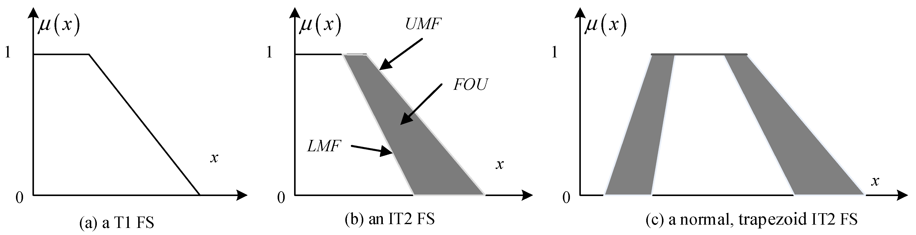
Figure 3.
Three types of FOUs and their parameters: (a) left-shoulder FOU; (b) interior FOU; and (c) right-shoulder FOU, adapted from [42].
Figure 3.
Three types of FOUs and their parameters: (a) left-shoulder FOU; (b) interior FOU; and (c) right-shoulder FOU, adapted from [42].

Figure 4.
IT2 FSs of five qualitative distance words for walk (unit: km).
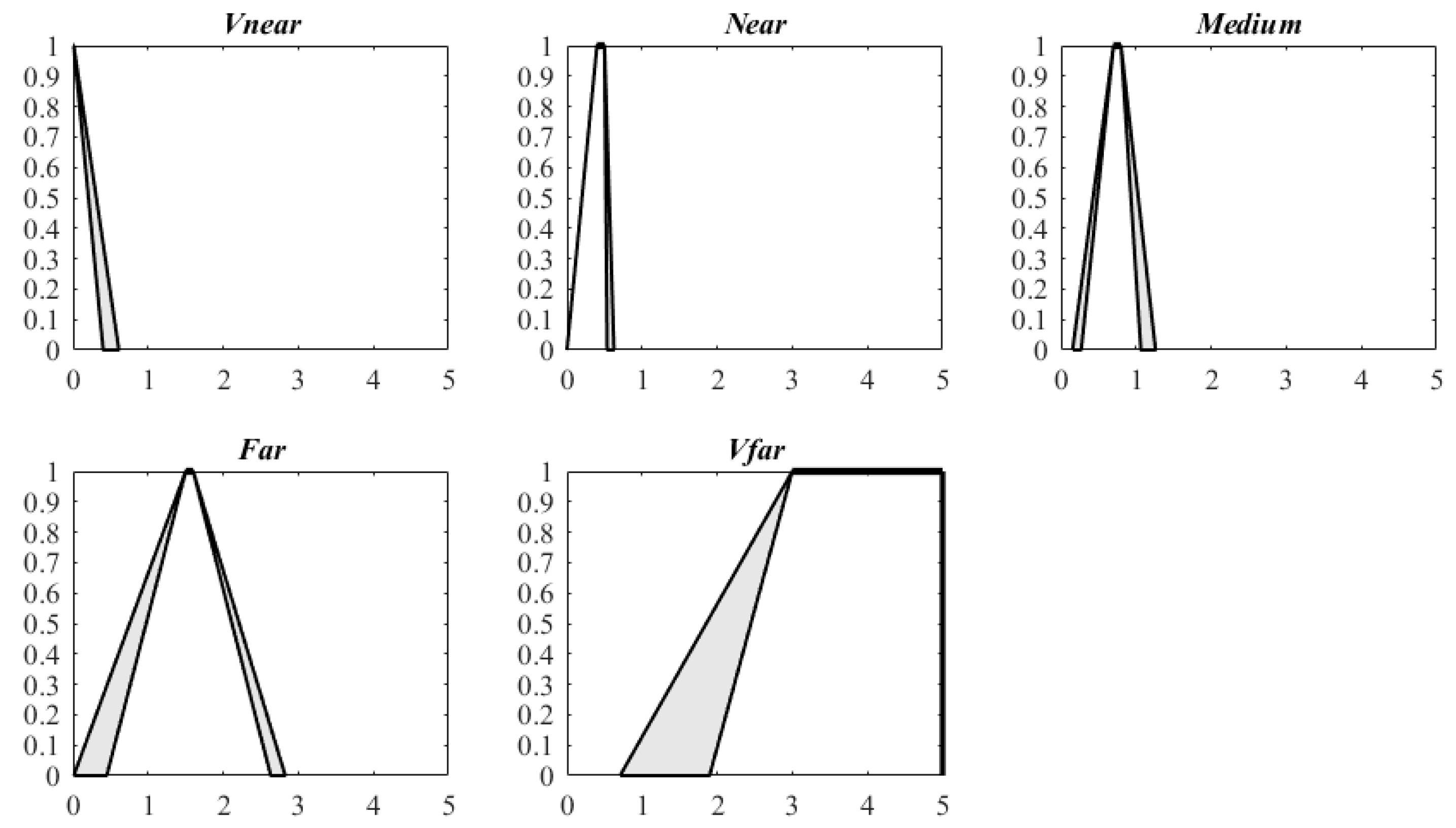
Figure 5.
IT2 FSs of five qualitative distance words for cycle (unit: km).
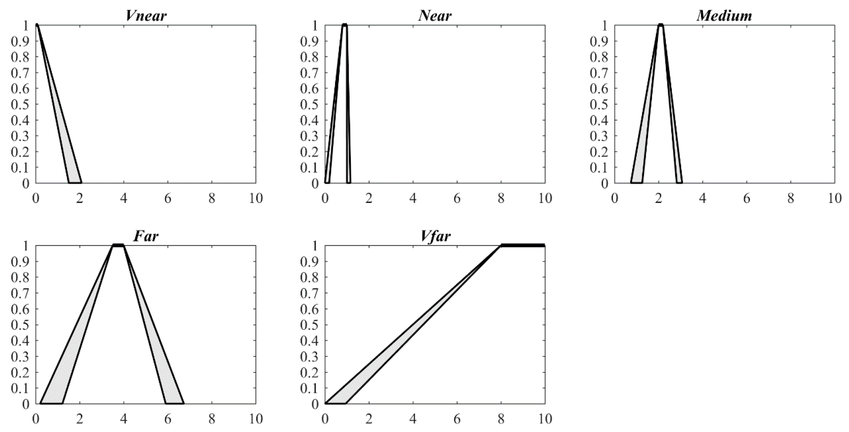
Figure 6.
IT2 FSs of five qualitative distance words for public transportation (unit: km).
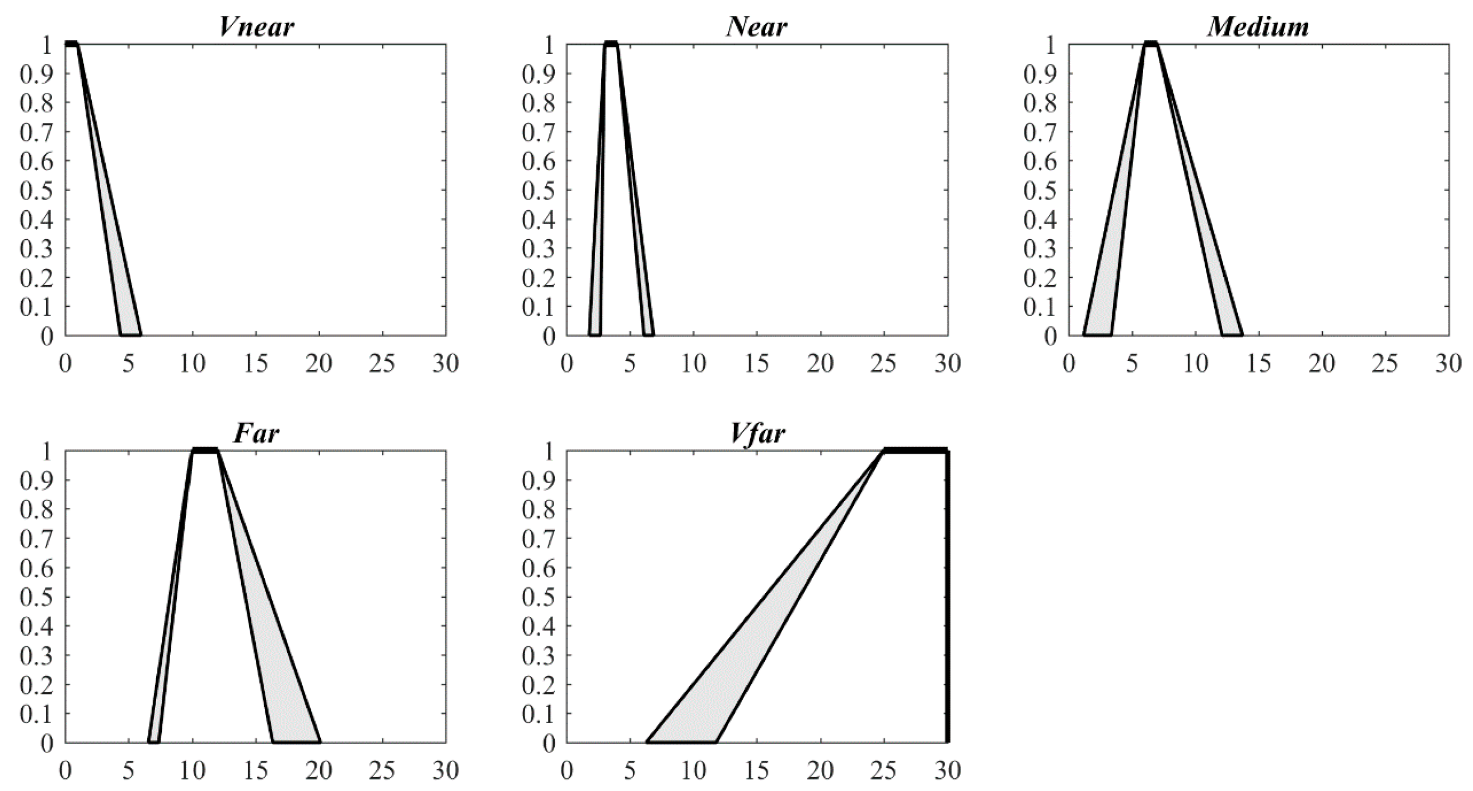
Figure 7.
IT2 FSs of five qualitative distance words for train (unit: km).
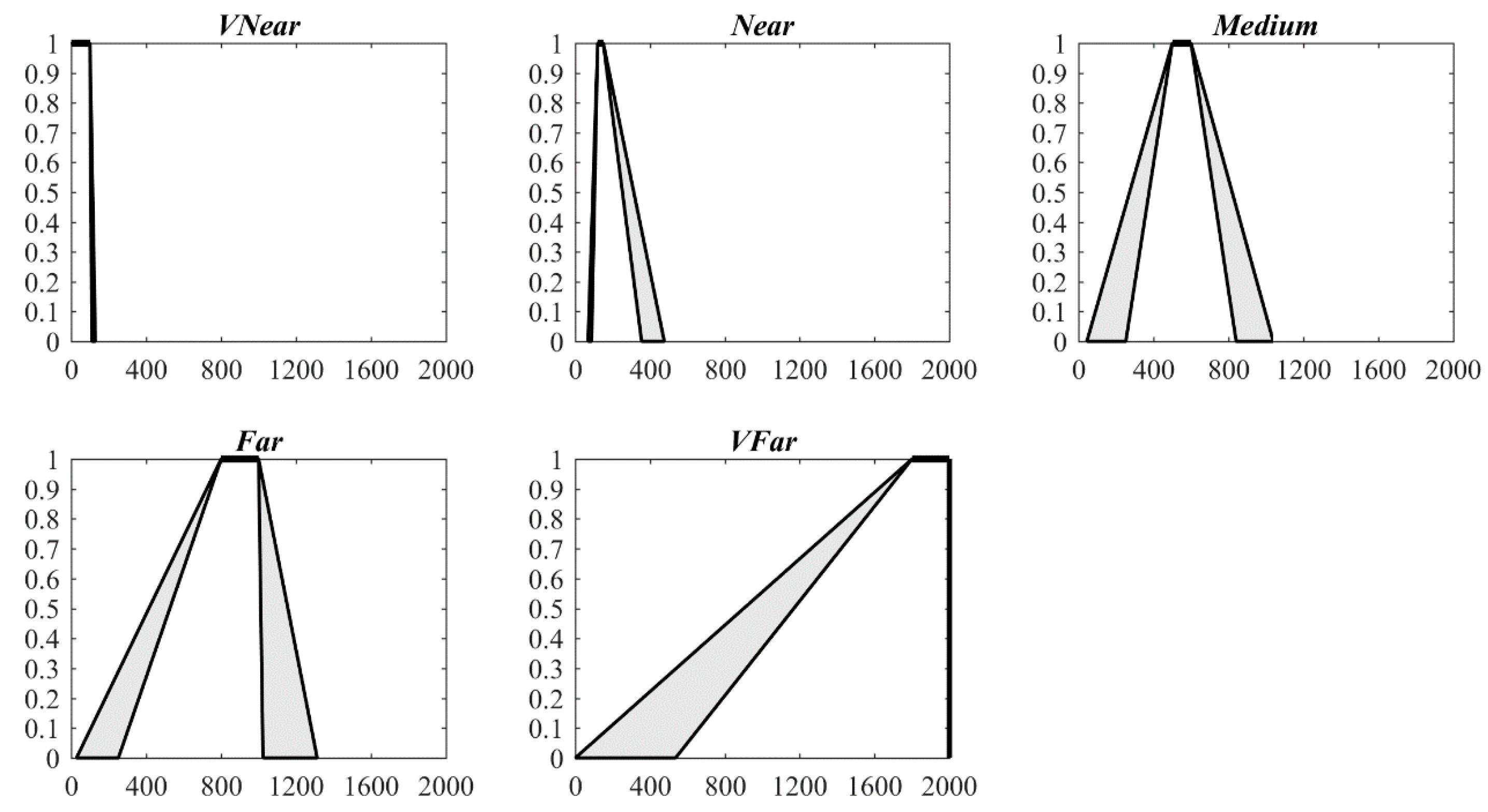
Figure 8.
Type-1 fuzzy sets modeling for distance words corresponding to two experts.

Figure 9.
Fuzzy interior division of the Haihe River, adapted from [33]: (a) Tianjin City river network; (b) upstream section; (c) midstream section; and (d) downstream section.
Figure 9.
Fuzzy interior division of the Haihe River, adapted from [33]: (a) Tianjin City river network; (b) upstream section; (c) midstream section; and (d) downstream section.

Figure 10.
The region with “medium” distance to the Haihe River by bicycle and the primary schools located in this region. (a) Lower membership grade of “medium” region; (b) upper membership grade of “medium” region; (c) the primary schools located in the “medium” region with upper membership grade greater than 0.5; (d) the primary schools located in the “medium” region with lower membership grade greater than 0.5.
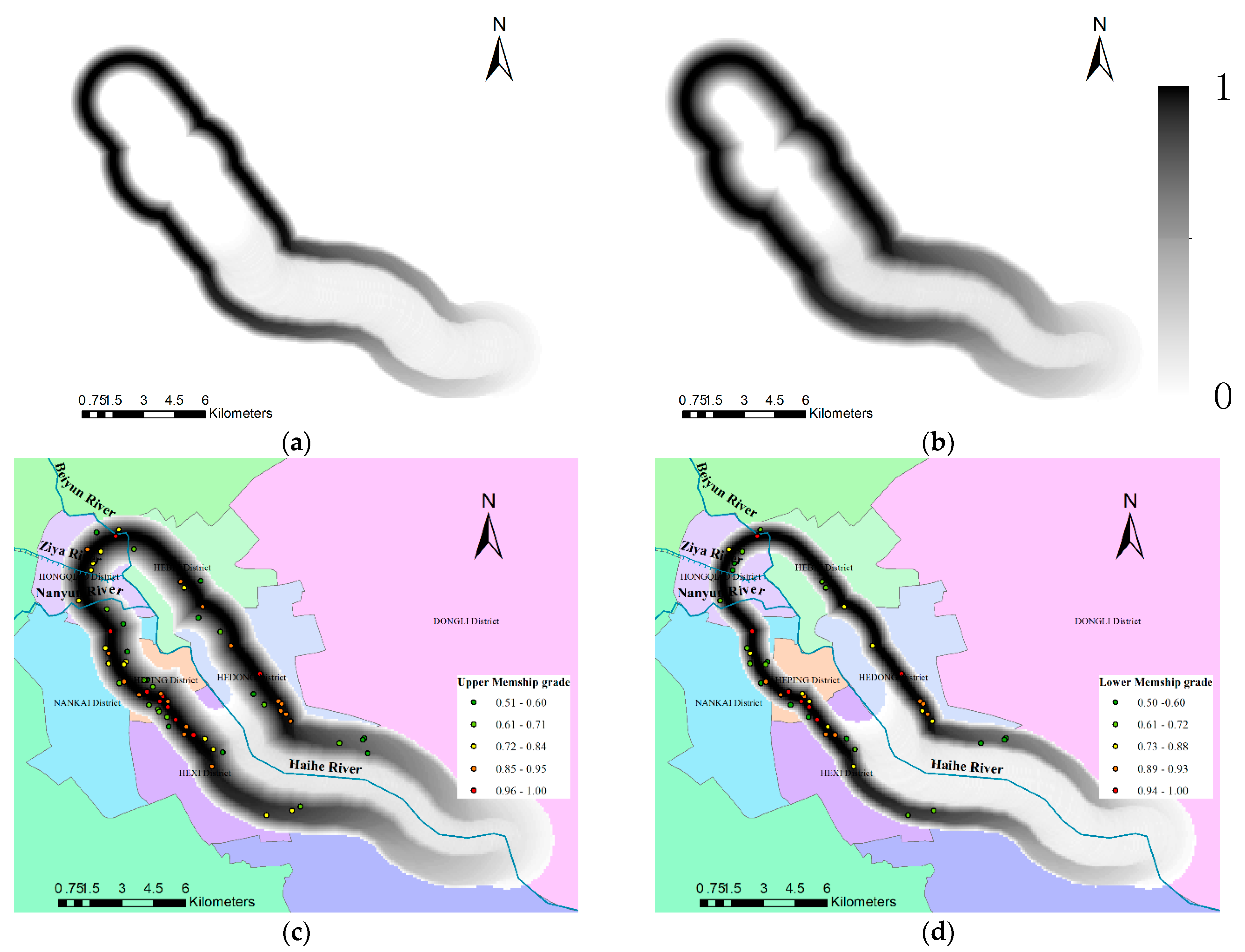
Table 1.
Parameters of IT2 FSs corresponding to five qualitative distance words for four travel modes.
Table 1.
Parameters of IT2 FSs corresponding to five qualitative distance words for four travel modes.
| Travel Mode | Distance Word | Parameters of UMF (km) | Parameters of LMF (km) | (km) | (km) | ||||||
|---|---|---|---|---|---|---|---|---|---|---|---|
| Walk | Vnear | 0.00 | 0.00 | 0.01 | 0.61 | 0.00 | 0.00 | 0.01 | 0.40 | 0.01 | 0.61 |
| Near | 0.00 | 0.40 | 0.50 | 0.63 | 0.00 | 0.40 | 0.50 | 0.54 | 0.10 | 0.63 | |
| Medium | 0.15 | 0.70 | 0.80 | 1.26 | 0.27 | 0.70 | 0.80 | 1.06 | 0.10 | 1.11 | |
| Far | 0.01 | 1.50 | 1.60 | 2.83 | 0.45 | 1.50 | 1.60 | 2.63 | 0.10 | 2.82 | |
| Vfar | 0.71 | 3.00 | 5.00 | 5.00 | 1.90 | 3.00 | 5.00 | 5.00 | 2.00 | 4.29 | |
| Cycle | Vnear | 0.00 | 0.00 | 0.10 | 2.09 | 0.00 | 0.00 | 0.10 | 1.51 | 0.10 | 2.06 |
| Near | 0.00 | 0.80 | 1.00 | 1.16 | 0.20 | 0.80 | 1.00 | 1.00 | 0.20 | 1.16 | |
| Medium | 0.74 | 2.00 | 2.20 | 3.07 | 1.26 | 2.00 | 2.20 | 2.83 | 0.20 | 2.33 | |
| Far | 0.20 | 3.50 | 4.00 | 6.74 | 1.22 | 3.50 | 4.00 | 5.91 | 0.50 | 6.53 | |
| Vfar | 0.00 | 8.00 | 10.00 | 10.00 | 0.94 | 8.00 | 10.00 | 10.00 | 4.00 | 9.26 | |
| Public transportation | Vnear | 0.00 | 0.00 | 1.00 | 6.02 | 0.00 | 0.00 | 1.00 | 4.39 | 1.00 | 6.08 |
| Near | 1.78 | 3.00 | 4.00 | 6.85 | 2.66 | 3.00 | 4.00 | 6.10 | 1.00 | 5.06 | |
| Medium | 1.20 | 6.00 | 7.00 | 13.73 | 3.39 | 6.00 | 7.00 | 12.12 | 1.00 | 12.53 | |
| Far | 6.59 | 10.0 | 12.00 | 20.12 | 7.41 | 10.0 | 12.00 | 16.34 | 2.00 | 12.22 | |
| Vfar | 6.27 | 25.0 | 30.0 | 30.00 | 11.79 | 25.0 | 30.00 | 30.00 | 5.00 | 23.73 | |
| Train | Vnear | 0 | 0 | 100 | 129 | 0 | 0 | 100 | 110 | 100.0 | 130.10 |
| Near | 68.6 | 120 | 150 | 476.1 | 87.4 | 120 | 150 | 354.9 | 30.00 | 415.20 | |
| Medium | 44.1 | 500 | 600 | 1039 | 251.9 | 500 | 600 | 841 | 100.0 | 1009.4 | |
| Far | 28.2 | 800 | 1000 | 1313 | 251.8 | 800 | 1000 | 1023 | 200.0 | 1438.8 | |
| Vfar | 0 | 1800 | 2000 | 2000 | 536 | 1800 | 2000 | 2000 | 300.0 | 1913.6 | |
Table 2.
Uncertainty indices of IT2 FSs corresponding to five distance words for four travel models modeled by the HMA and improved HMA.
Table 2.
Uncertainty indices of IT2 FSs corresponding to five distance words for four travel models modeled by the HMA and improved HMA.
| Travel Mode | Uncertainty Index | HMA | Improved HMA | ||||||||||
|---|---|---|---|---|---|---|---|---|---|---|---|---|---|
| Vnear | Near | Medium | Far | Vfar | Total | Vnear | Near | Medium | Far | Vfar | Total | ||
| Walk | Area of FOU | 0.05 | 0.10 | 0.28 | 1.00 | 0.83 | 2.26 | 0.10 | 0.05 | 0.16 | 0.32 | 0.60 | 1.22 |
| Fuzziness 1 | 0.34 | 0.31 | 0.32 | 0.35 | 0.36 | 1.70 | 0.35 | 0.22 | 0.33 | 0.35 | 0.36 | 1.61 | |
| Fuzziness 2 | 1.78 | 3.27 | 9.43 | 33.44 | 27.86 | 75.77 | 3.59 | 1.56 | 5.19 | 10.56 | 19.99 | 40.88 | |
| Variance | 0.01 | 0.02 | 0.05 | 0.35 | 0.36 | 0.79 | 0.02 | 0.02 | 0.04 | 0.27 | 0.25 | 0.59 | |
| Cycle | Area of FOU | 0.47 | 0.34 | 0.33 | 1.21 | 0.15 | 2.50 | 0.29 | 0.18 | 0.38 | 0.92 | 0.47 | 2.24 |
| Fuzziness 1 | 0.34 | 0.30 | 0.33 | 0.34 | 0.37 | 1.68 | 0.34 | 0.36 | 0.32 | 0.34 | 0.37 | 1.73 | |
| Fuzziness 2 | 5.98 | 4.50 | 4.14 | 15.27 | 1.86 | 31.76 | 3.75 | 3.61 | 4.89 | 11.54 | 5.87 | 29.65 | |
| Variance | 0.22 | 0.05 | 0.17 | 1.42 | 3.39 | 5.26 | 0.19 | 0.05 | 0.17 | 1.38 | 3.17 | 4.96 | |
| Public transportation | Area of FOU | 0.74 | 1.80 | 3.48 | 3.06 | 4.26 | 13.35 | 0.82 | 0.81 | 1.90 | 2.30 | 2.76 | 8.58 |
| Fuzziness 1 | 0.30 | 0.29 | 0.34 | 0.31 | 0.36 | 1.61 | 0.30 | 0.29 | 0.34 | 0.31 | 0.37 | 1.61 | |
| Fuzziness 2 | 3.00 | 7.30 | 14.04 | 12.41 | 17.05 | 53.82 | 3.38 | 3.29 | 7.72 | 9.33 | 11.05 | 34.78 | |
| Variance | 1.52 | 1.07 | 5.96 | 6.16 | 18.37 | 33.09 | 1.55 | 0.88 | 5.04 | 6.18 | 15.73 | 29.38 | |
| Train | Area of FOU | 20.13 | 10.35 | 168.96 | 469.50 | 280.13 | 949.08 | 9.49 | 70.04 | 202.93 | 256.37 | 267.98 | 806.81 |
| Fuzziness 1 | 0.10 | 0.31 | 0.33 | 0.32 | 0.37 | 1.43 | 0.06 | 0.33 | 0.33 | 0.31 | 0.37 | 1.39 | |
| Fuzziness 2 | 1.31 | 0.56 | 9.50 | 26.47 | 15.56 | 53.40 | 0.56 | 3.94 | 11.42 | 14.39 | 14.89 | 45.20 | |
| Variance | 884 | 5557 | 28156 | 74643 | 145232 | 254472 | 867 | 6240 | 28931 | 53368 | 145663 | 235068 | |
Table 3.
The primary schools located in the “medium” distance to the upstream of the Haihe River which is modeled as IT2 FS.
Table 3.
The primary schools located in the “medium” distance to the upstream of the Haihe River which is modeled as IT2 FS.
| ID | Name | Lower Membership Grade | Upper Membership Grade | Error of Membership |
|---|---|---|---|---|
| 8511245 | YONG JI XIAO XUE | 1.0000 | 1.0000 | 0.0000 |
| 8515596 | YUE YANG DAO XIAO XUE | 1.0000 | 1.0000 | 0.0000 |
| 8530346 | YI YANG XIAO XUE | 1.0000 | 1.0000 | 0.0000 |
| 8406934 | TAO HUA YUAN XIAO XUE | 1.0000 | 1.0000 | 0.0000 |
| 8540833 | KUN MING LU XIAO XUE | 0.9849 | 0.9899 | 0.0050 |
| 8510894 | YUAN CHENG XIAO XUE | 0.9803 | 0.9816 | 0.0013 |
| 8512237 | HUA XIA WEI LAI YI SHU XIAO XUE | 0.9270 | 0.9791 | 0.0521 |
| 8542812 | SHANG HAI DAO XIAO XUE | 0.9661 | 0.9774 | 0.0113 |
| 8514663 | KUN MING LU XIAO XUE | 0.9568 | 0.9767 | 0.0199 |
| 8520570 | YUE YANG DAO XIAO XUE | 0.9166 | 0.9551 | 0.0385 |
| 8514586 | XIN XING XIAO XUE | 0.9213 | 0.9475 | 0.0262 |
| 8538733 | EN DE LI XIAO XUE | 0.8736 | 0.9326 | 0.0590 |
| 8513199 | YI YANG XIAO XUE | 0.8721 | 0.9312 | 0.0590 |
| 8514613 | DONG FANG XIAO XUE | 0.8954 | 0.9303 | 0.0349 |
| 8519552 | SI HAO LU XIAO XUE | 0.8939 | 0.9288 | 0.0349 |
| 8537185 | SHANG HAI DAO XIAO XUE FEN XIAO | 0.8939 | 0.9288 | 0.0349 |
| 8426650 | HU ZHU DAO XIAO XUE | 0.8643 | 0.9259 | 0.0616 |
| 8538022 | TIAN JIN SHI SHI YAN XIAO XUE | 0.8609 | 0.9251 | 0.0642 |
| 8426553 | HU ZHU DAO XIAO XUE | 0.9239 | 0.9239 | 0.0000 |
| 8509788 | HE DONG SHI YAN XIAO XUE | 0.8534 | 0.9211 | 0.0677 |
| 8513580 | KUN WEI LU YI XIAO | 0.8534 | 0.9211 | 0.0677 |
| 8508222 | HAI YANG YI XIAO JIAO XUE QU | 0.8661 | 0.9107 | 0.0446 |
| 8539007 | WU MA LU XIAO XUE | 0.8661 | 0.9107 | 0.0446 |
| 8533082 | QIU ZHEN XIAO XUE | 0.8661 | 0.9107 | 0.0446 |
| 8418068 | ZHONG XIN DONG DAO XIAO XUE | 0.8986 | 0.8986 | 0.0000 |
| 8469819 | HE MU DAO XIAO XUE | 0.8986 | 0.8986 | 0.0000 |
| 8512972 | LI SHUI DAO XIAO XUE | 0.8811 | 0.8811 | 0.0000 |
| 8408161 | YOU AI DAO XIAO XUE | 0.8691 | 0.8691 | 0.0000 |
| 8509640 | KUN WEI LU YI XIAO | 0.7183 | 0.8483 | 0.1300 |
| 8536258 | NAN KAI ZHONG XIN XIAO XUE | 0.6984 | 0.8376 | 0.1392 |
| 8515544 | JIAN SHAN XIAO XUE | 0.6167 | 0.8285 | 0.2118 |
| 8510652 | HE BEI QU DI ER SHI YAN XIAO XUE | 0.6703 | 0.8224 | 0.1522 |
| 8538777 | XIN CUN XIAO XUE | 0.6703 | 0.8224 | 0.1522 |
| 8522712 | TIAN JIN SHI DA DI ER FU XIAO | 0.5965 | 0.8114 | 0.2148 |
| 8512402 | HONG HU LI XIAO XUE | 0.5714 | 0.7692 | 0.1978 |
| 8512553 | SHAO GONG ZHUANG XIAO XUE | 0.6390 | 0.7593 | 0.1203 |
| 8515227 | WU MA LU XIAO XUE | 0.6355 | 0.7570 | 0.1215 |
| 8424178 | YU YING LI XIAO XUE | 0.6355 | 0.7570 | 0.1215 |
| 8531501 | YA XI YA XIAO XUE | 0.5376 | 0.7510 | 0.2134 |
| 8538975 | WU MA LU XIAO XUE | 0.6081 | 0.7387 | 0.1306 |
| 8411260 | LING SHUI DAO XIAO XUE | 0.6865 | 0.7369 | 0.0504 |
| 8514552 | NAN KAI ZHONG XIN XIAO XUE | 0.5076 | 0.7348 | 0.2273 |
| 8411750 | ZHU JIANG DAO XIAO XUE | 0.7249 | 0.7249 | 0.0000 |
| 8513795 | WEN CHANG GONG MIN ZU XIAO XUE | 0.4684 | 0.7138 | 0.2454 |
| 8511466 | NAN KAI ZHONG XIN XIAO XUE | 0.5402 | 0.6935 | 0.1533 |
| 8514988 | WAI YU XUE YUAN FU ER XIAO | 0.5402 | 0.6935 | 0.1533 |
| 8538703 | MA CHANG DAO XIAO XUE | 0.5402 | 0.6935 | 0.1533 |
| 8411270 | DONG HAI LI XIAO XUE | 0.3633 | 0.6930 | 0.3297 |
| 8514270 | WEN SHAN LI XIAO XUE | 0.4016 | 0.6778 | 0.2762 |
| 8511329 | XI KANG LU XIAO XUE | 0.5000 | 0.6667 | 0.1667 |
| 8517795 | QIAN CHENG XIAO XUE | 0.3789 | 0.6656 | 0.2866 |
| 8510697 | HU ZHU DAO XIAO XUE | 0.2631 | 0.6493 | 0.3862 |
| 8510891 | DA QIAO DAO XIAO XUE | 0.2631 | 0.6493 | 0.3862 |
| 8408068 | ER HAO QIAO XIAO XUE | 0.5244 | 0.6473 | 0.1230 |
| 8538694 | KUN MING LU XIAO XUE | 0.4602 | 0.6401 | 0.1799 |
| 8511172 | TIAN TAI XIAO XUE | 0.3282 | 0.6382 | 0.3101 |
| 8509898 | HE PING QU XIN ZHONG XIAO XUE | 0.2857 | 0.6154 | 0.3297 |
| 8510408 | KUN MING LU XIAO XUE | 0.4175 | 0.6117 | 0.1942 |
| 8511274 | NING YUAN XIAO XUE | 0.3979 | 0.5986 | 0.2007 |
| 8509892 | HE PING QU ZHONG XIN XIAO XUE | 0.2032 | 0.5709 | 0.3678 |
| 8540181 | ZHONG YING XIAO XUE | 0.2032 | 0.5709 | 0.3678 |
| 8408448 | WU SHI XIAO XUE | 0.5642 | 0.5655 | 0.0013 |
| 8511404 | DA QIAO DAO XIAO XUE | 0.1169 | 0.5485 | 0.4316 |
| 8531345 | HONG XING XIAO XUE | 0.3205 | 0.5470 | 0.2265 |
| 8408042 | HE DONG WU SHI XIAO XUE | 0.5440 | 0.5440 | 0.0000 |
| 8514559 | HONG YUAN LI XIAO XUE | 0.1326 | 0.5330 | 0.4003 |
| 8426222 | JIN MEN XIAO XUE | 0.0824 | 0.5170 | 0.4345 |
| 8519570 | TONG WANG XIAO XUE | 0.2665 | 0.5110 | 0.2445 |
| 8522698 | XIN SHI JI XIAO XUE | 0.1178 | 0.5088 | 0.3910 |
| 8522746 | TIAN JIN SHI DA DI ER FU XIAO | 0.1178 | 0.5088 | 0.3910 |
| 8510681 | QI ZHI XUE XIAO | 0.0859 | 0.5078 | 0.4219 |
© 2018 by the authors. Licensee MDPI, Basel, Switzerland. This article is an open access article distributed under the terms and conditions of the Creative Commons Attribution (CC BY) license (http://creativecommons.org/licenses/by/4.0/).
Share and Cite
MDPI and ACS Style
Guo, J.; Du, S. Modeling Words for Qualitative Distance Based on Interval Type-2 Fuzzy Sets. ISPRS Int. J. Geo-Inf. 2018, 7, 291. https://doi.org/10.3390/ijgi7080291
AMA Style
Guo J, Du S. Modeling Words for Qualitative Distance Based on Interval Type-2 Fuzzy Sets. ISPRS International Journal of Geo-Information. 2018; 7(8):291. https://doi.org/10.3390/ijgi7080291
Chicago/Turabian StyleGuo, Jifa, and Shihong Du. 2018. "Modeling Words for Qualitative Distance Based on Interval Type-2 Fuzzy Sets" ISPRS International Journal of Geo-Information 7, no. 8: 291. https://doi.org/10.3390/ijgi7080291
Note that from the first issue of 2016, this journal uses article numbers instead of page numbers. See further details here.