
A Method of Ship Detection under Complex Background

1
University of Chinese Academy of Sciences, Beijing 100049, China
2
Changchun Institute of Optics, Fine Mechanics and Physics, Chinese Academy of Sciences, Dongnanhu Street, Changchun 130033, China
*
Author to whom correspondence should be addressed.
ISPRS Int. J. Geo-Inf. 2017, 6(6), 159; https://doi.org/10.3390/ijgi6060159
Submission received: 30 March 2017
/
Revised: 18 May 2017
/
Accepted: 28 May 2017
/
Published: 31 May 2017
Abstract
:The detection of ships in optical remote sensing images with clouds, waves, and other complex interferences is a challenging task with broad applications. Two main obstacles for ship target detection are how to extract candidates in a complex background, and how to confirm targets in the event that targets are similar to false alarms. In this paper, we propose an algorithm based on extended wavelet transform and phase saliency map (PSMEWT) to solve these issues. First, multi-spectral data fusion was utilized to separate the sea and land areas, and the morphological method was used to remove isolated holes. Second, extended wavelet transform (EWT) and phase saliency map were combined to solve the problem of extracting regions of interest (ROIs) from a complex background. The sea area was passed through the low-pass and high-pass filter to obtain three transformed coefficients, and the adjacent high frequency sub-bands were multiplied for the final result of the EWT. The visual phase saliency map of the product was built, and locations of ROIs were obtained by dynamic threshold segmentation. Contours of the ROIs were extracted by texture segmentation. Morphological, geometric, and 10-dimensional texture features of ROIs were extracted for target confirmation. Support vector machine (SVM) was used to judge whether targets were true. Experiments showed that our algorithm was insensitive to complex sea interferences and very robust compared with other state-of-the-art methods, and the recall rate of our algorithm was better than 90%.
1. Introduction
Ship targets are a key objective of maritime surveillance and wartime combat, and the automatic detection and identification of ships is of great practical significance with wide applicability in both civilian and military domains. There have been many previous studies on ship detection in synthetic aperture radar (SAR) images. These kinds of methods have advantages in that they are little affected by weather and time, but they are limited due to low SAR image resolution and a long revisit period [1,2,3]. In recent years, with the rapid development of optical remote imaging technology, some researchers have paid more attention to the detection of ships with optical images due to their higher spatial resolution and more detailed spatial contents, when compared with SAR images [4,5,6,7,8].
In comparison to SAR detection algorithms, ship detection algorithms (based on optical remote-sensing images) are more recent. At present, the methods for ship detection can be generalized from three aspects: sea and land separation, candidate target positioning, and false alarm removal. In the first stage, separation methods aim to separate the sea from the land area quickly by using intensity threshold segmentation, regional growth, and prior geographic information [9,10]. The main purpose of the second stage is to search out all candidate regions that include ship targets as much as possible, based on gray-level analysis, shape and edge features, and machine vision perception [11,12,13]. Reference [11] proposed a discrimination mechanism of sliding window pixels at the stage of ROIs positioning and selected ship candidates by morphological filtering. Reference [12] located small ship candidates through a Bayesian decision. Previous work on distinguishing ships from false alarms have mainly used the advantage of some machine learning methods [14,15,16], such as support vector machine (SVM) and neural networks, by extracting features and binary classification.
Due to optical imaging conditions, cloud cover, wake, noise, and other interferences, it is difficult to distinguish between the ships and the background, and ship targets can even submerge in the complex background. This has resulted in little work done in the field of detecting ships under complex sea surfaces. The saliency segmentation framework has been used to find potential suspicious targets under the premise that the separation of land and sea is handled in advance, and the structure-LBP (Local Binary Patterns) feature was proposed to confirm real ships [17]. Characteristics of gray and texture features have been adopted to extract potential target areas, and to remove false alarms, several geometrical features have been extracted during post-processing and SVM was used to train and predict the uncertain ship targets [18]. A ship detection method with broken cloud interference was proposed in Reference [19], and the double-parameter constant false alarm rate (CFAR) was used to detect ROIs. This method uses the gray-scale difference of the search window and the target window to position, so the model is less robust when the image brightness changes suddenly, or the target edge is quite blurred.
In summary, the complexity of optical images increases the difficulty of detection and while most of the proposed methods perform well with image of simple sea–land situations, there is still room for improvement. To further investigate the problems arising from optical panchromatic images, a hierarchical method is utilized in this paper, including three stages: pre-processing, prescreening, and post-processing. The outline of this paper is organized as follows. Section 2 details the method of ship extraction, and focuses on how to use the proposed method to locate ROIs in cluttered scenes and to select features to eliminate false alarms. Section 3 shows the parameter selection for our method, the experimental results of ship detection performed on remote sensing images, and compares our results with other methods. Finally, Section 4 provides a discussion and the conclusions of our study.
2. Proposed Method
2.1. A Whole Process
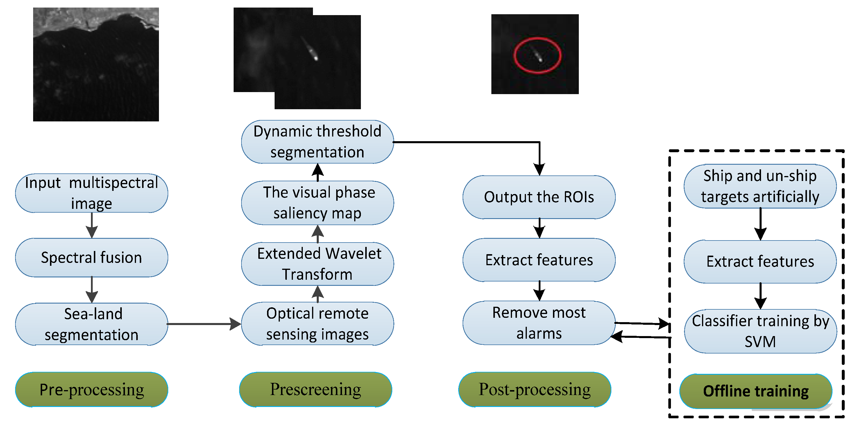
When considering the complex background of various interferences, we allowed more suspicious targets in the pre-screening stage and stripped out false alarms as much as possible in the post-processing stage. Figure 1 shows the flowchart of our proposed detection algorithm. First, we rapidly separated the sea from the land using multi-spectral information. Second, in this stage, a novel method of ROI extraction based on EWT was conducted, and the transformation result was used to construct a significant map of the phase spectrum. Next, we obtained a binary image by dynamic threshold segmentation to locate the ROIs. Finally, at the post-processing stage, besides commonly used shape and gray distribution features, the texture feature of the Gray Level Co-occurrence Matrix (GLCM) and the rotation-invariant unified local binary pattern of improved LBP () were introduced to improve the adaptability and robustness of the training model for different types of remote sensing images. We used the SVM classification approach (based on multiple extracted features) to distinguish between ships and non-ships to remove most of the false alarms.
2.2. Pre-Processing Stage
For a given image, we performed sea–land segmentation using spectral fusion. Multispectral images (produced by the same camera with optical remote sensing images) have different reflection characteristics at different wave bands, so have different digital numbers. The reflection of water gradually weakens from the visible wavelengths to the infrared wavelengths. The absorption of water is stronger in the near-infrared band; however, the reflection of vegetation is strongest in this band. Thus, we made full use of this information to separate the sea and land by using the Normalized Difference Water Index (NDWI) [20], and its formula is
where and are the row and column on the multispectral image. and represent the digital number of green band and near-infrared band, respectively. On the sea surface, the digital number of the green band () is much larger than that of the near infrared band (). While on the land, is less than . is within −1–+1, is a binary image after segmentation, and is the threshold got by statistics. Based on those natures, the sea–land region is divided initially by . As shown in Figure 2b, white and black areas denote the sea and land, respectively. Red oval circles are holes resulting from the segmentation. We removed hollows in the land and islands in the sea by the morphological corrosion and expansion method, so the broken areas were combined into one object as shown in Figure 2c. In addition, the method could remove some thick clouds, as shown in Figure 3.
2.3. Prescreening
The location of ROIs under complex sea conditions is the core of the target detection algorithm. As the sea surface is greatly influenced by weather, capture conditions, sea waves, and other factors, wakes and intensities of ships differ under different imaging conditions. To solve this problem, this paper proposed the use of EWT; thus, on this basis, we constructed a significant map of the phase spectrum to locate the ROIs. This method is referred to as PSMEWT (Phase Saliency Map Based Extended Wavelet Transform, PSMEWT).
2.3.1. The Theory of the Proposed PSMEWT Method
Discrete wavelet transform (DWT) has the strong ability to characterize the local characteristics of the signal in the time and frequency domain, which is useful in detecting the transience or singularity of the signal [21]. DWT is based on the idea of a tree-structure filter, which is implemented through the loop iteration of image down-sampling and filtering. The relationship between the adjacent scale decomposition factors is expressed as
where and denote the low pass and high pass quadrature mirror filter, respectively. denotes an image; and and denote the decomposition factors of the scale of j.
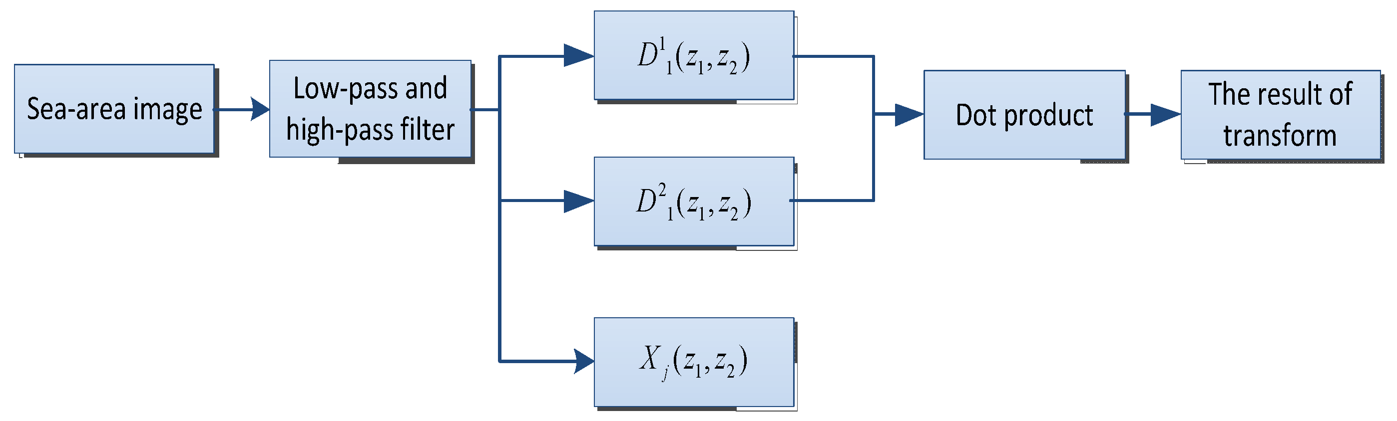
However, the process of DWT reduces spatial resolution of the original image, which can be harmful for image target detection and recognition. Thus, this paper proposed EWT. First, we made an image pass through the low-pass and high-pass filters to obtain three transformed coefficients of low frequency coefficients , the high frequency vertical detail , and the horizontal detail . The calculation process is
where and represent horizontal and vertical directions, respectively. denotes the input image. The horizontal and vertical coefficients on adjacent scales are the same as the original image, without resolution reduction. Meanwhile, based on the propagation properties of signals and noise between different scales, we multiply the absolute value of horizontal high-frequency coefficients and vertical high-frequency coefficients to reduce the influence of image noise on target detection and enhance the edge gradient value of targets, simultaneously. The calculation process of EWT is shown in Figure 4.
As the Harr wavelet basis has the simultaneous advantages of orthogonality and symmetry, there is no displacement on the same breakpoint at different scales [21]. This paper used the Harr wavelet basis for EWT, , . The main feature of this method was to enhance the contrast between the ships and the background.
Second, we constructed a phase significance map from the results of the EWT to locate the ROIs as the frequency domain significance map is suitable for detecting small targets in sparse scenes, and ships are small–scale targets in a large number of sea data [22]. The method is able to quickly remove large areas of the background and improve the detection rate of the algorithm. We conducted a Fourier transform of the results of the EWT, and calculated the phase spectrum. Next, a Fourier inverse transform of the phase spectrum was performed. Finally, we used a Gaussian smoothing filter on the result. The calculation process of the significance map is
where and represent the two-dimensional Fourier transform and inverse transform, respectively. is the image of phase spectrum. denotes the significant map after transformation. denotes the Gaussian low-pass filter function. is the result of the EWT.
Finally, we used the adaptive dynamic threshold method to segment the phase significant map to obtain the positions of the ROIs. The threshold is calculated as
where and represent the mean and variance of the phase significant map, respectively. is an empirical adjustment coefficient. indicates the threshold of dynamic segmentation. is a binary image. After threshold segmentation, one centroid point was used to express adjacent regionals. With this point as the center, the image was cut into many suspicious target slices.
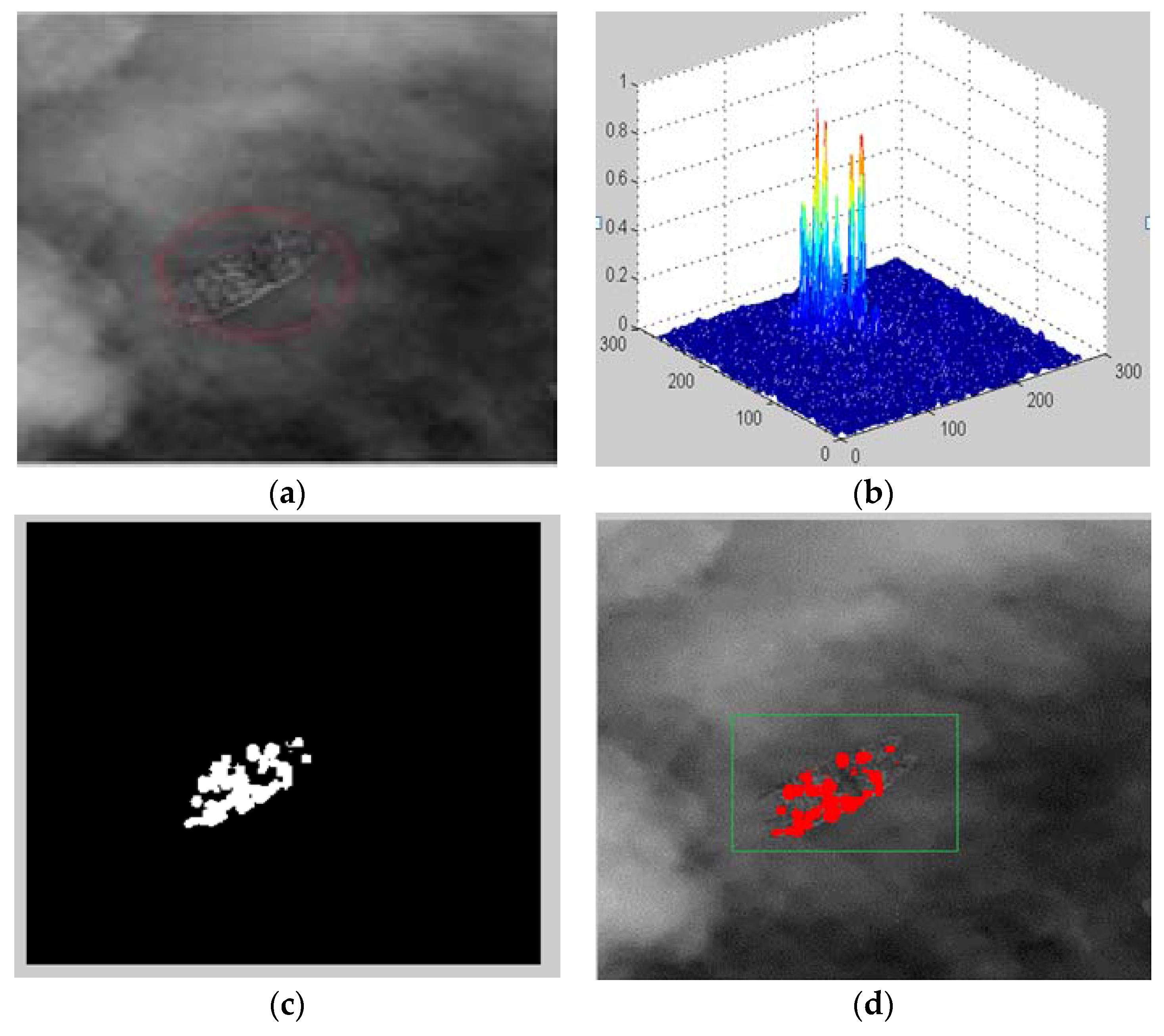
As seen in Figure 5, Figure 5a is the original image of the ship in clouds, and Figure 5b is the three-dimensional show of the phase significant map after PSMEWT transformation. We can see that the significant value of the target was significantly higher than the background. Figure 5c is the result of threshold segmentation and we located the ROI denoted by the green box in Figure 5d.
2.3.2. Comparative Experiments of Different Location Algorithms
• Comparison between DWT and EWT
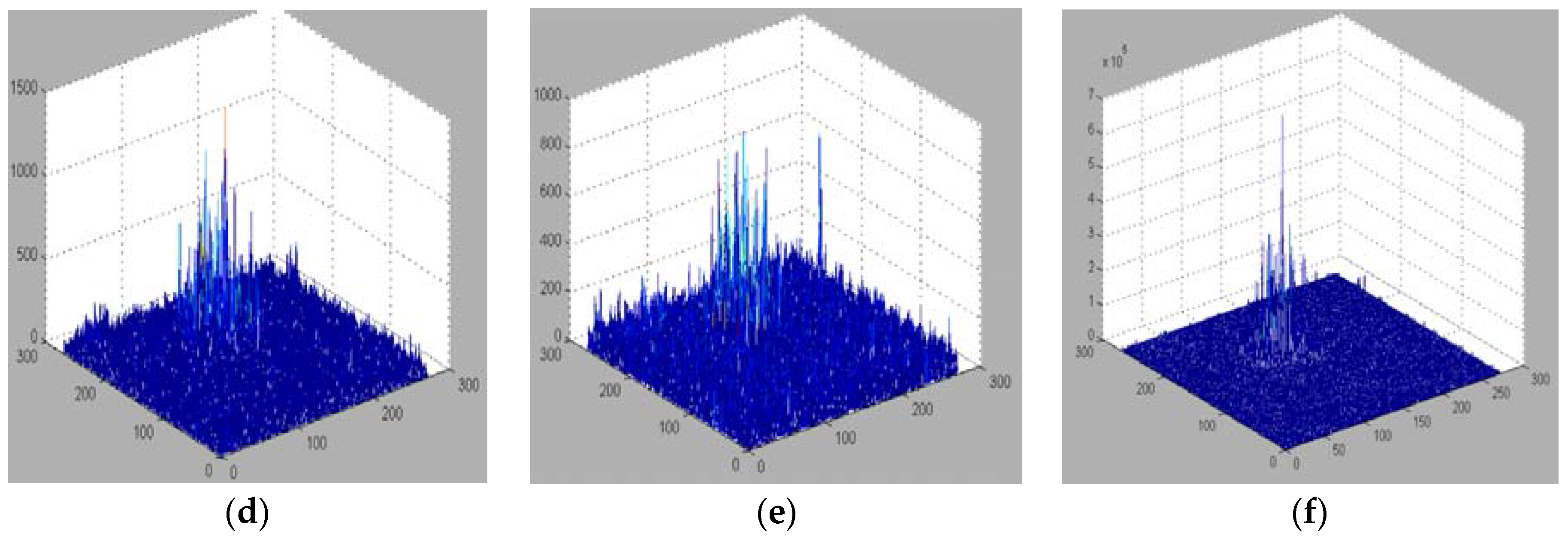
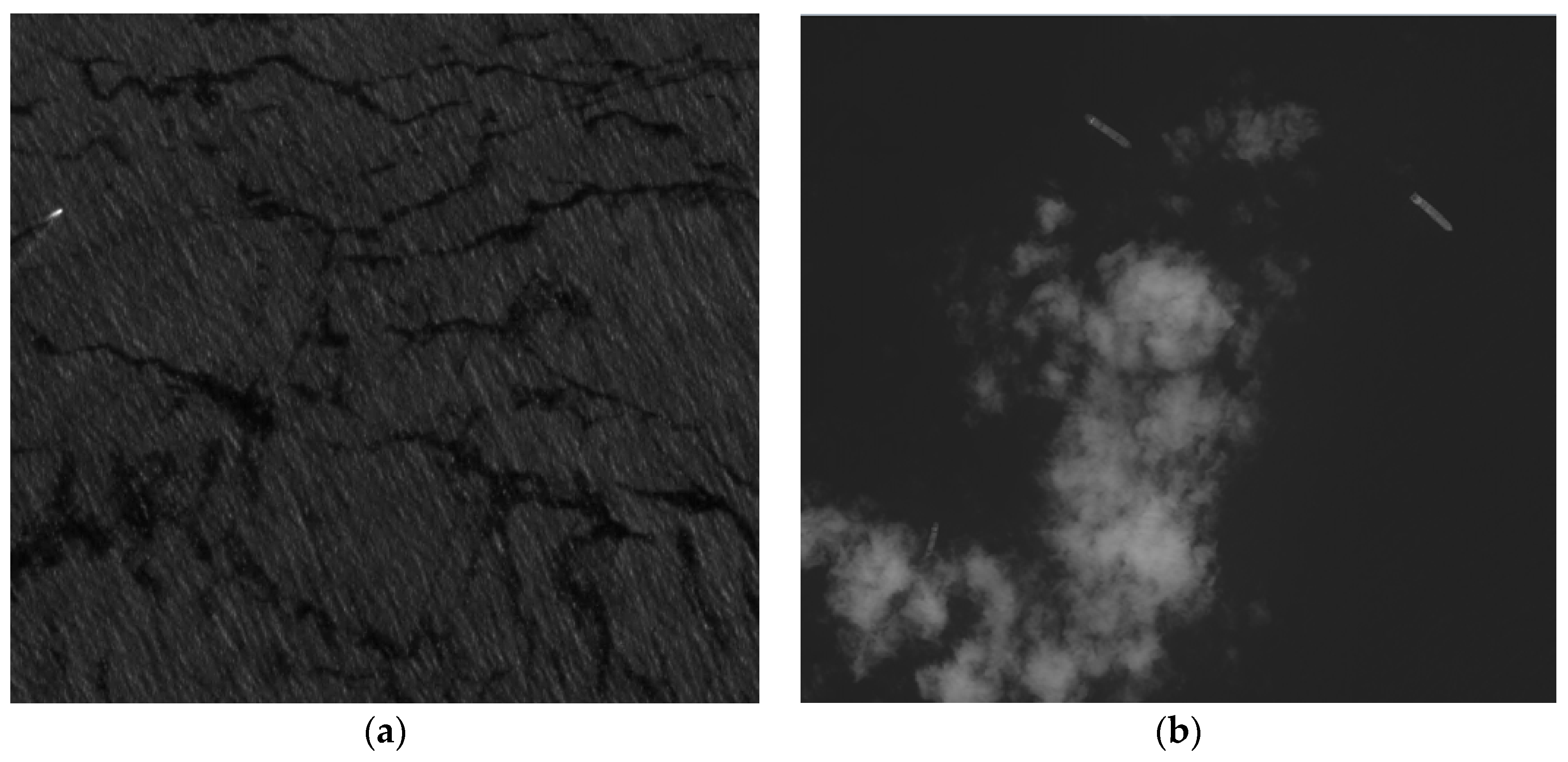
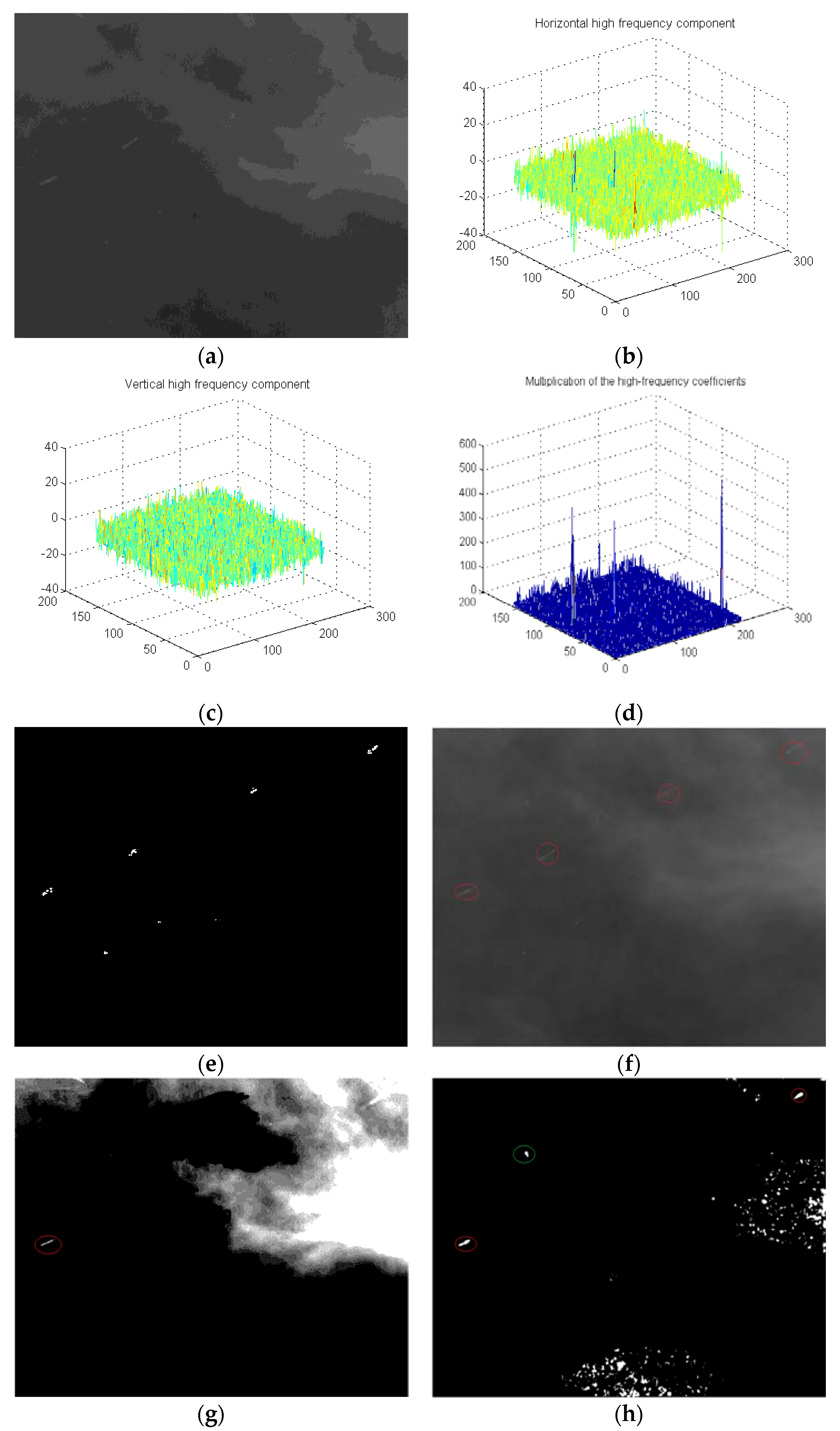
To verify the validity of the proposed EWT in this paper for location of the ROIs, DWT and EWT were performed on the same image. Figure 6a is an image containing two ships submerged in a thick cloud. Horizontal and vertical high frequency components of the DWT are shown in Figure 6b,c, where there is no clear boundary between the coefficients of targets and the background. After the multiplication of adjacent high frequency sub-bands by EWT transformation, the target coefficient was significantly prominent, which made it easy to detect targets, as shown in Figure 6f.
• Comparative experiments between PSMEWT and traditional localization methods on different sea conditions
Optical remote sensing images with a 2–5 m resolution downloaded from Google Earth were used as experiment images. The localization method of PSMEWT proposed in this paper was compared with common localization methods, including the Otsu-based threshold segmentation method and the Canny-based edge detection method.
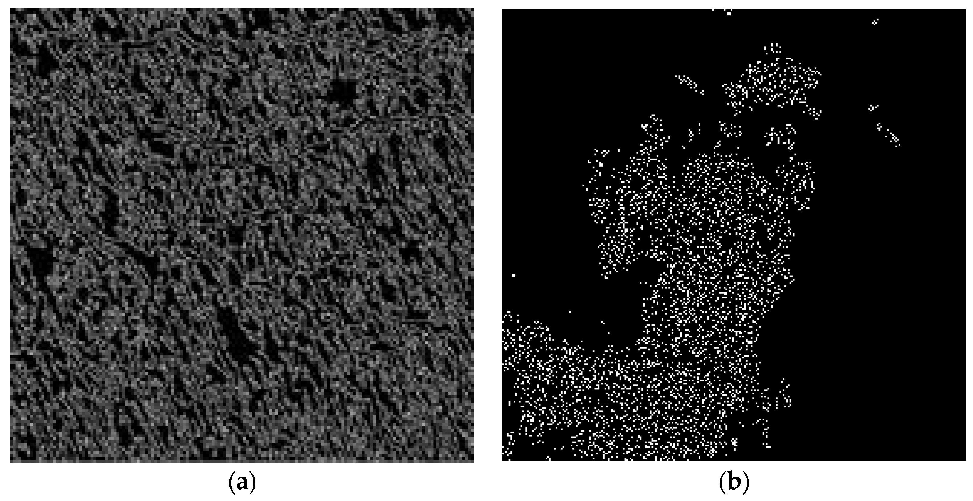
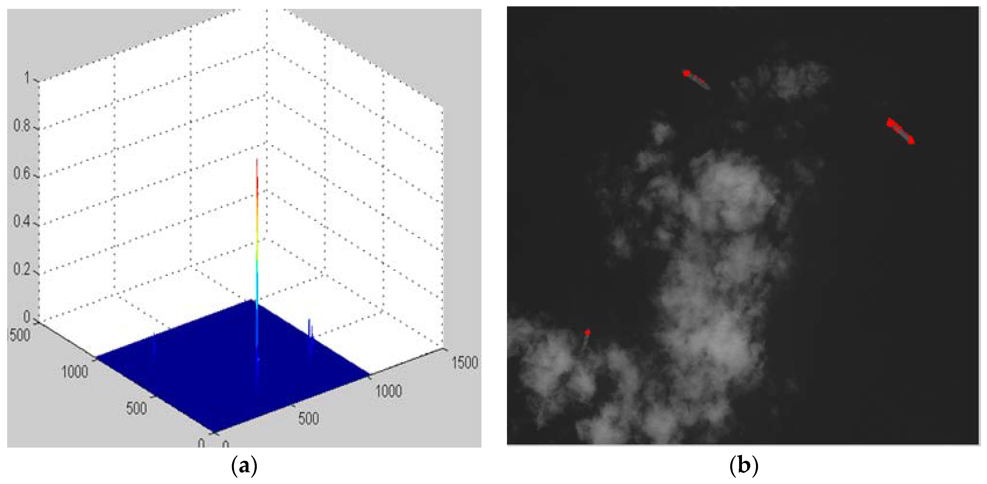
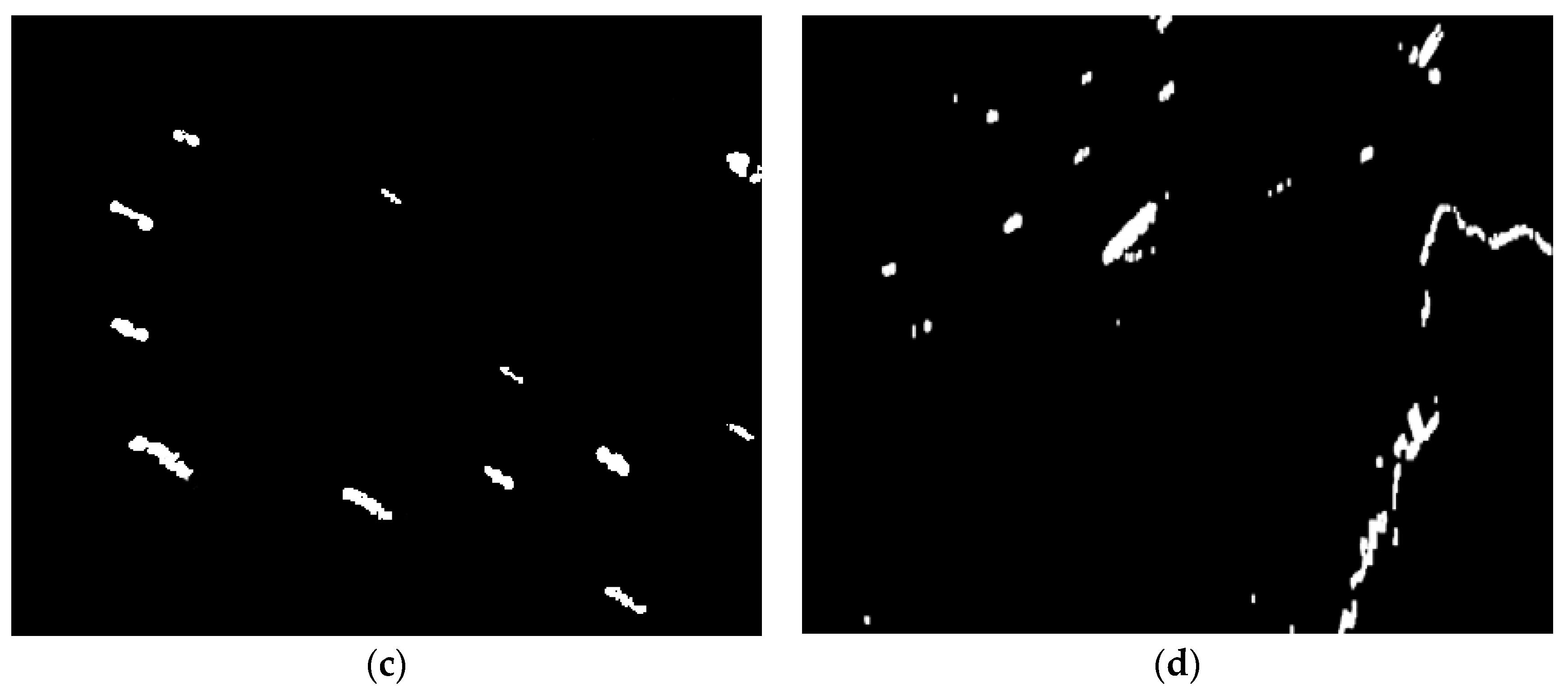
Figure 7 shows the original images to be detected, and the experimental results of the three algorithms are shown in Figure 8, Figure 9, Figure 10 and Figure 11. The image becomes a binary image after Otsu processing (as shown in Figure 8a,b), and the white areas denote suspicious positions that the algorithm has located. For Figure 8a, this algorithm is insufficient to locate targets in such cases. As shown in Figure 9a,b, the phenomenon of boundary confusion existed between the Canny results of target and background, and was invalid in suspected target positioning. Figure 10 and Figure 11 show the three-dimensional significant maps and positioning results after PSMEWT. Compared with traditional methods, the PSMEWT method could successfully extract all ships under complicated scenes and avoid missing potential candidates.
2.4. Post-Processing
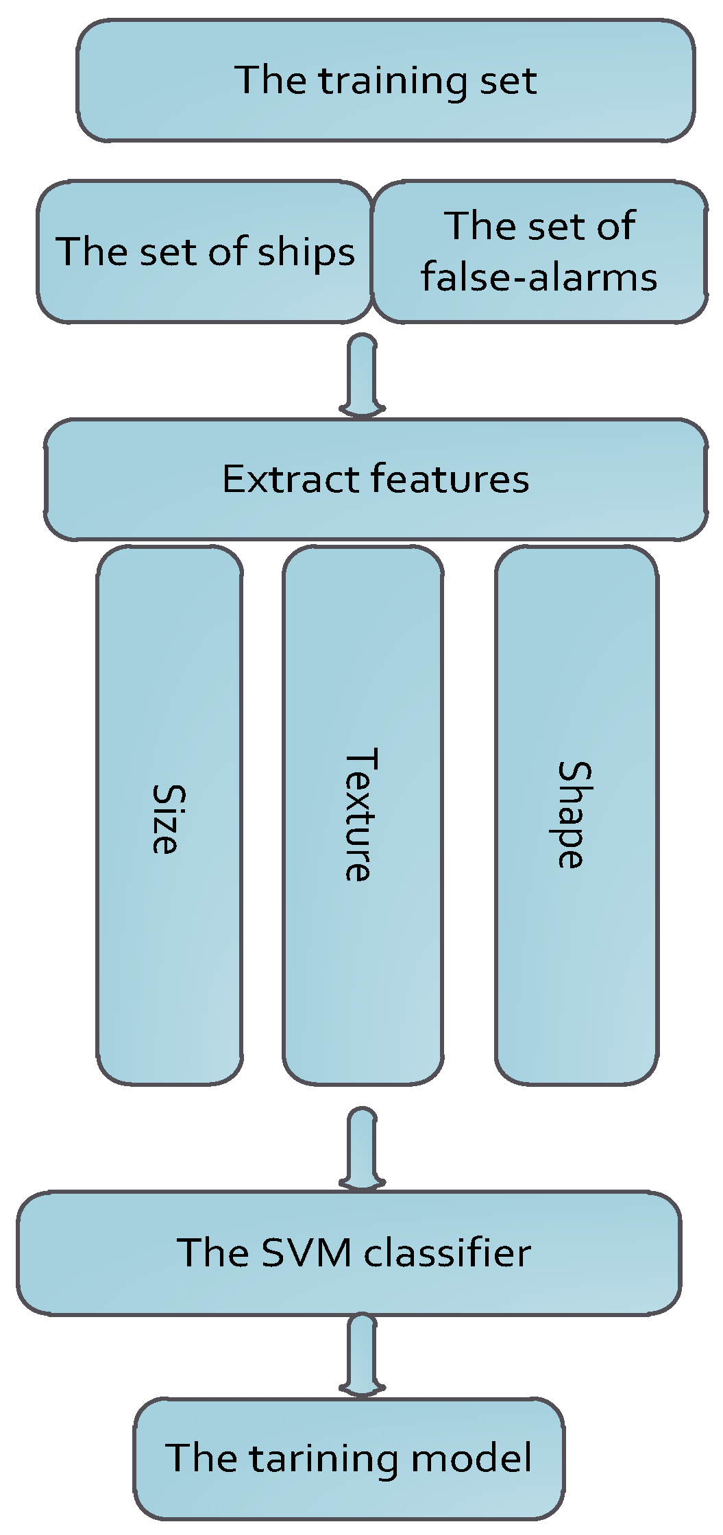
Post-processing is conducted to gather features of slice images to further weed out false alarms. One key issue was to find efficient feature descriptors to characterize ship targets. By using the above-mentioned steps, we could obtain the center of mass points from the ROIs, and use these points as the starting points to spread around and extract contours of slice images using the texture segmentation method presented in Reference [23]. Next, features were extracted from the obtained contours and original slices for SVM training, as shown in Figure 12. In this paper, three types of 10-dimensional features were extracted from one slice, including size, shape, and texture features. The detection model was established from the training samples of ships and false alarms through SVM offline training.
The shape features used in the training included length, width, area, and perimeter. Furthermore, we selected three morphological features to eliminate false alarms, including length–width ratio, compactness, and rectangularity. They can be calculated as
where H is the length of the connected area; W is the width of the connected area; P is the perimeter of the contour; and S is the number of the connected area points.
At the same time, we used the contrast and correlation of the GLCM [24] to describe texture, as calculated below
where is an element of GLCM; is the average of GLCM, ; and is the standard deviation, .
In addition, the difference in texture distribution was described by calculating the histogram variance of . is the rotation-invariant unified local binary pattern of the improved LBP [25], and can detect the basic attributes of a local texture image such as bright spots and dark spots. It can be calculated as
where s(x) is the binary sign function; is the number of exchanges between 0 and 1 (N-digit binary figures), , . and denote the value of the center pixel value and neighbor pixels, respectively.
As ships are usually thin and long, we used simple shape features such as area, length, width, and to directly eliminate more obvious false alarms, for example, islands and big clouds. When considering the texture distribution, and GLCM were introduced to strengthen the ability to describe ships and non-ships. Figure 13 shows extracted samples of the SVM training from space-borne optical images where Figure 13a gives various ship samples, and Figure 13b shows several typical false-alarm samples. We randomly extracted ships, waves, and clouds from their training samples, and each sample size was 20. We calculated the variance value of the histogram and the correlation value () of GLCM, obtaining the results seen in Figure 14. The statistics chart of histogram variance is shown in Figure 14a, and the ship texture distribution was greatly different. In contrast, the texture of waves and clouds changed slowly. It can be seen in Figure 14a that the value of ships (red line) was far above the values of the clouds and waves (green line and blue line). The correlation of GLCM was used to measure the similar degree of GLCM elements in the row or column directions. When the matrix elements of GLCM were uniform, the absolute value of correlation was very high; however, if the matrix elements of GLCM varied widely, it was relatively low. As we can see in Figure 14b, the correlation value is negative and the absolute value of correlation of clouds and waves is larger (green line and blue line) than that of ships (red line).
It was easy to find that features in use were effective enough to distinguish ships from false alarms by the statistical experiments mentioned above. Both shape and texture attributes of the candidate slices were adopted to SVM classification, and the combined features could improve the adaptability and robustness of the training model.
3. Experimental Results and Performance Comparison
To evaluate the applicability of the algorithm, three groups of images were downloaded from Google Earth: a quiet sea with a sea surface with few interferences (Group 1); a textured sea with visible swell or thick cloud (Group 2); and a cluttered sea, the sea surface with many interferences (Group 3). The spatial resolutions ranged from 1 to 5 m. The proposed method was implemented in C++ with Intel (R) Xeon (R) CPU at 2.40 GHz and 64.0 GB RAM.
We used metrics of Recall and Precision to quantitatively evaluate the algorithm’s performance.
where TP is the number of correctly identified targets; FP is the number of background objects mistaken as targets; and FN is the number of targets mistaken as background objects.
3.1. Parameter Selection
Due to the different resolutions of the experimental images and various image conditions, texture and other characteristic values differed across images of various resolution. To achieve a low missing rate, we set different thresholds. SVM was adopted as the basic classifier in our two-class classification problem. We selected the training set through two steps. The first step screening was performed in principal computer (PC). We detected ROIs from the optical images and obtained slices of candidates by the proposed PMEWT method. We calculated simple shape features of each slice, including length, width, area, compactness, and rectangularity. We conducted a secondary artificial screening of candidates that met the threshold conditions. We set different thresholds based on different image resolutions. Using 2 m resolution images as an example, the ranges of length, width, area, and perimeter were set to 200–20, 70–10, 14,000–200, and 540–60, respectively. Length–width ratio ranged from 1.25 to 16, rectangularity ranged from 0.4 to 1, and compactness was greater than or equal to 15. Those thresholds set at different resolutions were defined by summarizing many ship candidates and reading related references. The second step screening was performed by humans. For slices selected by PC, we classified them via an artificial mechanism, and selected ship and non-ship targets. There was a total of 1050 samples, including 480 ship slices, 260 cloud slices, 230 wave slices, and 80 other slices, with 480 total positive samples and 570 negative samples. Out of these totals, we randomly selected 336 positive samples and 399 negative samples as the training set based on 70% of all slices, and the others were selected as the test set.
Prior to training, we linearly normalized each feature to the range (0, 1). The main advantage of normalization was to avoid feature attributes in greater numeric ranges dominating those in smaller numeric ranges. We chose the radial basis function (RBF) as the kernel function as it nonlinearly maps samples into a higher dimensional space, so it could handle cases when the relationships between class labels and attributes were nonlinear [26]. There are two key parameters for the RBF kernel: and . is the penalty parameter of the error term; and is the parameter of the kernel formula. We obtained the best parameters through the cross-validation method [26] and set and . In addition, the parameter used in sea–land segmentation was set to 0.3. The parameter k in the adaptive dynamic threshold method was set to three. Based on the experience of multiple experiments, we calculated the values of GLCM in four directions (0°, 45°, 90°, 135°), and then used the mean value as the final parameters of each slice.
3.2. Contrastive Experiments
We carried out experiments on 290 images with a 2048×4096-pixel size. We tested our approach on three groups of different sea surfaces (which have been previously explained at the beginning Section 3). The total number of ship targets in Group 1, Group 2, and Group 3 was 133, 143, and 78, respectively; the number of detected targets in Group 1, Group 2 and Group 3 was 135, 151, and 90, respectively; and the number of real targets in Group 1, Group 2 and Group 3 was 130, 131, and 64, respectively.
We can see from Table 1 that with an increasing number of interferences, the value of Recall and Precision decreased slightly from Group 1 to Group 3, but the average of Recall could reach up to 90.46% for different sea surfaces, and the average of Precision was 84.72% even in the case of very complex sea surfaces. These results demonstrate the effectiveness and applicability of our method.
To verify that the proposed method had a positive impact on ship detection, we compared our method with the state-of-the-art methods proposed in References [17,18] on Recall and Precision. These experiments were conducted on 290 images of the different situations above-mentioned, including the quiet sea, textured sea, and cluttered sea. The Recall and Precision of the method used in Reference [17] were 87.65% and 80.47%, respectively, while the Recall and Precision of the method in Reference [18] were 80.08% and 78.92%, respectively. In contrast, our method achieved a detection effect with higher accuracy.
Here, we present one contrastive result of the three methods. As shown in Figure 15a, the image is of four ships on the sea covered by thin clouds, where the contrast of target and background is very low. Figure 15b,c are the three-dimensional map of horizontal transformation coefficients by EWT and the three-dimensional map of vertical transformation coefficients by EWT, respectively. We obtained the final result of the EWT by dot product of horizontal transformation coefficients and vertical transformation coefficients, and the three-dimensional map is shown in Figure 15d. We constructed a phase significant map and obtained a binary segmentation image, as shown in Figure 15e. At this step, tone can obtain both the ships’ position and the locations of the non-ships simultaneously. Finally, some false alarms were removed and the final ship targets confirmed, as shown in Figure 15f. As we can see from Figure 15b, the raised positions are the locations of targets, and the contrast of target and background was significantly enhanced after dot product of horizontal and vertical transformation coefficients. This highlighted the targets from the background and made it easy to find targets in the phase significance map. We located four ships accurately by binary segmentation of the phase significance map and rejected two false alarms through features extracted from the ROIs. It also showed the effectiveness of the features used in our paper. Although ships are weakly contrasted with the background, our method achieved good detection results.
Reference [18] combined the gray-scale difference map with the texture difference map to separate targets from the background. The gray-scale difference map was obtained by subtracting the mean value of one image from the original image. The larger values of the gray-scale difference map are more likely to be targets. Local Walsh transform was used for the texture difference map. Coefficients of the local Walsh transformation were constructed by the gray value difference between the center pixel and eight other points in the neighborhood. False alarms were eliminated by basic shape features, such as length, width, and area. As seen in Figure 15g, we used the method in Reference [13] to conduct binary segmentation of the ROIs, where one ship target was detected and the other three were missed. There are two reasons for this result. One is that both the gray-scale difference map and the texture difference map use the gray difference value between the center point and neighborhood points. When the gray difference of the whole image changes little, it is difficult to detect targets. The other cause is that it is not sufficiently reliable to reject false alarms using only simple shape features in a complex scene.
Reference [17] integrated intensity distinctness and the significant map into the process of ship detection. ROIs were obtained by dynamic threshold segmentation, and shape features and the structure LBP of ships were used to determine whether the candidate was a real ship. The structure LBP separately extracted LBP histogram features on different regions, including the prow, left hull, right hull, and stern. As shown in Figure 15h, we used the method proposed in Reference [12] to obtain binary segmentation of the ROIs. Two ship targets were detected and the other two were missed. At the same time, one false alarm was detected. Influenced by the illumination and weather, the intensity of ships is similar to that of the background. In such cases, the intensity difference is insufficient to detect ships and it is difficult to highlight targets in the background despite combining intensity distinctness with the significant map. Furthermore, structural LBP mainly suits big ships as there is no significant difference in the LBP distribution of the prow, left hull, right hull, and stern when the ship is small and relatively blurred. It is unreliable in distinguishing between small ships from similar false alarms by the structural LBP.
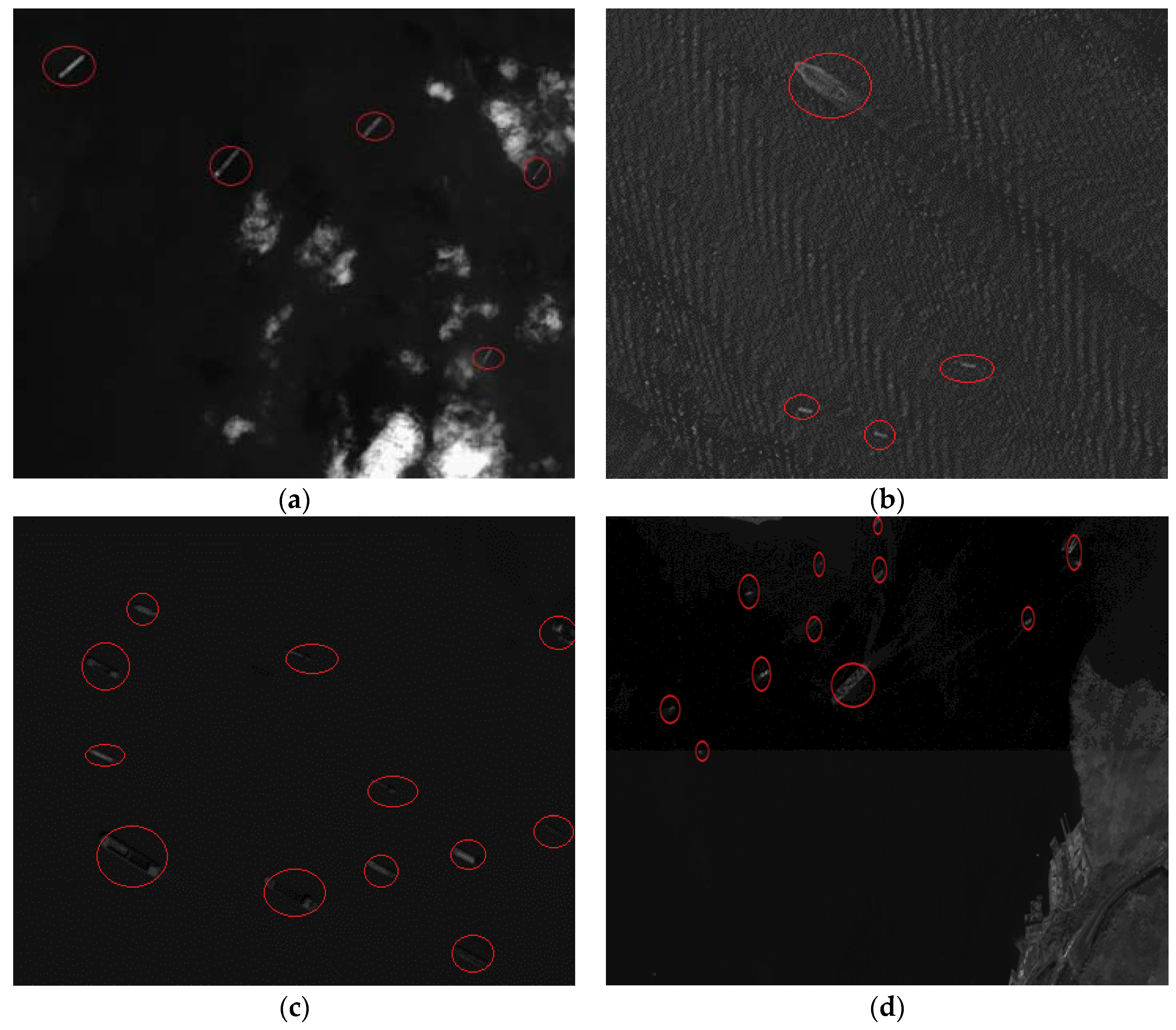
Due to space limitations, we only present four detected results of our method. Figure 16 shows some typical sea surfaces. Figure 17 provides the corresponding processing results of the visual phase saliency images, and Figure 18 shows the detected results of different cases.
Figure 16a shows an image where one ship is half-shaded by clouds, whose texture and gray value are similar to ships. Figure 16b is an image with very dramatic change in the partial area. Many wave fringes increase the false alarm targets. Figure 16c shows ships of low contrast on the sea surface, which increases the difficulty of detection. Figure 16d is an image of a simple sea surface.
Figure 17 shows the results of sea area images processed through PSMEWT and dynamic threshold segmentation, and white areas denote the ROIs. It is clearly observed from Figure 17 that the ROI localization method based on PSMEWT is very accurate without missed alarms. This is because the EWT method enhances the edge and contrast of targets, and makes the target position more prominent by combining it with the significance map of phase spectrum. Although there were some false alarms in the process of the land and sea separation and PSMEWT, the 10-dimension feature vectors adopted by our method were effective enough to remove most of the false alarms, as shown in Figure 18.
4. Conclusions
Ships play an important role in both civil and military fields. Traditional methods do not perform very well under a complex sea surface. We proposed a method named PSMEWT. Multi-spectral information was first adopted in the sea–land segmentation to reduce the detection time consumption. Then we constructed a visual phase saliency map based on the extended wavelet transform to highlight the difference between ships and the background to locate ship candidates. In the process of removing false alarms, aside from morphological and geometric features, we introduced the GLCM and to more effectively eliminate false alarms, and the SVM classifier was adopted to conduct offline training at the same time. Extensive experiments validated our method, which not only outperformed the present ship detection methods on precision and recall, but was also robust for complex background interference.
However, there is still room for improvement. There will be relatively more false targets when our method is applied to small ships. The small size (only 10–20 pixels) of the ships in the images makes it difficult to determine whether it is a ship through optical remote sensing images. Further study will be required into methods to improve the precision and recall. In addition, the multi-spectral fusion method was adopted in sea–land segmentation because our camera had many channels; however, it can be replaced by other methods and will not affect the subsequent use of our algorithm.
Acknowledgments
This work was supported in part by the Science and Technology Development Program of Jilin under Grant 20170204029GX. The first author would like to thank Bin He of Changchun Institute of Optics, Fine Mechanics and Physics, Chinese Academy of Sciences for his valuable assistance and guidance. The authors wish to thank the associate editor and the anonymous reviewers for their valuable suggestions.
Author Contributions
Both authors worked on the proposal of the method. Ting Nie proposed the idea of the method. Wensheng Wang and Ting Nie performed conceived experiment. Ting Nie designed and performed the experiments. Bin He, Guoling Bi and Yu Zhang analyzed the data. Ting Nie wrote the paper and all the authors read and approved the final paper.
Conflicts of Interest
The authors declare no conflict of interest.
References
- Eldhuset, K. An automatic ship and ship wake detection system for space borne SAR images in coastal regions. IEEE Trans. Geosci. Remote Sens. 1996, 34, 1010–1019. [Google Scholar] [CrossRef]
- Wang, X.L.; Chen, C.X. Ship detection for complex background SAR images based on a multiscale variance weighted image entropy method. IEEE Geosci. Remote Sens. Lett. 2017, 14, 184–187. [Google Scholar] [CrossRef]
- Wang, S.G.; Wang, M.; Yang, S.Y.; Jiao, L.C. New hierarchical saliency filtering for fast ship detection in high-resolution SAR images. IEEE Geosci. Remote Sens. Lett. 2017, 55, 351–362. [Google Scholar] [CrossRef]
- Wu, W.; Luo, J.C.; Qiao, C. Ship recognition from high resolution remote sensing imagery aided by spatial relationship. In Proceedings of the IEEE International Conference on Spatial Data Mining and Geographical Knowledge Services (ICSDM), Fuzhou, China, 29 June–1 July 2011; pp. 567–569. [Google Scholar]
- Li, K.-D.; Zhang, Y.-Y.; Li, Y.-J. Researches of sea surface ship target auto-recognition based on wavelet transform. In Proceedings of the 2010 International Conference on System Science Engineering Design and Manufacturing Informatization, Yichang, China, 12–14 November 2010; pp. 193–195. [Google Scholar]
- Guo, J.; Zhu, C.R. A novel method of ship detection from space-borne optical image based on spatial pyramid matching. Appl. Mech. Mater. 2012, 190–191, 1099–1103. [Google Scholar] [CrossRef]
- Xu, Q.Z.; Li, B.; He, Z.F.; Ma, C. Multiscale contour extraction using level set method in optical satellite images. IEEE Geosci. Remote Sens. Lett. 2011, 8, 854–858. [Google Scholar] [CrossRef]
- Zhu, C.; Zhou, H.; Wang, R.; Guo, J. A novel hierarchical method of ship detection from spaceborne optical image based on shape and texture features. IEEE Trans. Geosci. Remote Sens. 2010, 48, 3446–3456. [Google Scholar] [CrossRef]
- Zhao, Y.-H.; Wu, X.-Q.; Wen, L.-Y.; Xu, S.-S. Ship target detection scheme for optical remote sensing images. Opto-Electron. Eng. 2008, 35, 105–109. [Google Scholar]
- Yang, G.; Li, B.; Ji, S.F. Ship detection from optical satellite images based on sea surface analysis. IEEE Geosci. Remote Sens. Lett. 2014, 11, 641–645. [Google Scholar] [CrossRef]
- Corbane, C. A complete processing chain for ship detection using optical satellite imagery. Int. J. Remote Sens. 2010, 31, 5837–5854. [Google Scholar] [CrossRef]
- Proia, N.; Page, V. Characterization of a Bayesian ship detection method in optical satellite images. IEEE Geosci. Remote Sens. Lett. 2010, 7, 226–230. [Google Scholar] [CrossRef]
- Li, S.; Zhou, Z.Q.; Wang, B.; Wu, F. A novel inshore ship detection via ship head classification and body boundary determination. IEEE Geosci. Remote Sens. Lett. 2016, 3, 1920–1924. [Google Scholar] [CrossRef]
- Yi, L.; Xu, S.-S. A new method for ship target recognition based on support vector machine. Comput. Simul. 2006, 6, 1006–9348. [Google Scholar]
- Vapnik, V.N. The Nature of Statistical Learning Theory; Springer: New York, NY, USA, 1995; pp. 358–450. [Google Scholar]
- Zou, Z.X.; Shi, Z.W. Ship detection in spaceborne optical image with SVD networks. IEEE Trans. Geosci. Remote. 2016, 54, 5832–5845. [Google Scholar] [CrossRef]
- Yang, F.; Xu, Q.Z.; Li, B. Ship detection from optical satellite images based on saliency segmentation and structure-LBP feature. IEEE Geosci. Remote Sens. Lett. 2017, 14, 1–5. [Google Scholar] [CrossRef]
- Yu, X.; Wan, S.H.; Yue, L.H. A novel algorithm for ship detection based on dynamic fusion model of multi-feature and support vector machine. In Proceedings of the 2011 Sixth International Conference on Image and Graphics, Hefei, China, 12–15 August 2011; pp. 521–526. [Google Scholar]
- Chen, H.-L.; Lei, L.; Shou, S.-L. A method of anti-disturbance by ragged clouds for detecting ships on the sea. Comput. Eng. Sci. 2010, 32, 46–49. [Google Scholar]
- Zhang, D.; Ni, Q.; Fang, D.; Li, J.H.; Yao, W.; Yuan, S.G. Application of multispectral remote sensing technology in surface water body extraction. In Proceedings of the 2016 International Conference on Audio, Language and Image Processing, Shanghai, China, 11–12 July 2016. [Google Scholar]
- Sidney, B.C.; Gopinath, R.A. Introduction to Wavelets and Wavelet Transforms: A Primer. Shengrui, G. (Translation); Publishing House of Electronics Industry: Beijing, China, 2013; pp. 34–40. [Google Scholar]
- Li, X.; Liu, Y.Q.; Bian, C.J. Inshore ship detection method in optical remote sensing images using local salient characteristics. J. Image Graph. 2016, 21, 657–664. [Google Scholar]
- Tanunchai, B.; Thanwa, S.; Sanun, S. Texture Segmentation using active contour model incorporated with edge flow on MRI image. In Proceedings of the TENCON 2014—IEEE Region 10 Conference, Bangkok, Thailand, 22–25 October 2014; pp. 1–5. [Google Scholar]
- Rakesh, A.; Ramesh, K.S.; Lakhan, D.S. Fog detection using GLCM based features and SVM. In Proceedings of the 2016 IEEE Conference on Advances in Signal Processing (CASP) Cummins College of Engineering for Women, Pune, India, 9–11 June 2016; pp. 72–76. [Google Scholar]
- Ojala, T.; Pietikäinen, M.; Mäenpää, T. Multiresolution gray-scale and rotation invariant texture classification with local binary pattern. IEEE Trans. Pattern Anal. Mach. Intell. 2002, 24, 971–987. [Google Scholar] [CrossRef]
- Bin, G.; Victor, S. Cross Validation through Two-Dimensional Solution Surface for Cost-Sensitive SVM. IEEE Trans. Pattern Anal. Mach. Intell. 2017, 39, 1103–1121. [Google Scholar]
Figure 1.
Flowchart of our proposed detection algorithm.

Figure 2.
Land-sea segmentation based on multi-spectral fusion. (a) Multi-spectral original image; (b) land-sea segmentation; and (c) hole filling.
Figure 2.
Land-sea segmentation based on multi-spectral fusion. (a) Multi-spectral original image; (b) land-sea segmentation; and (c) hole filling.
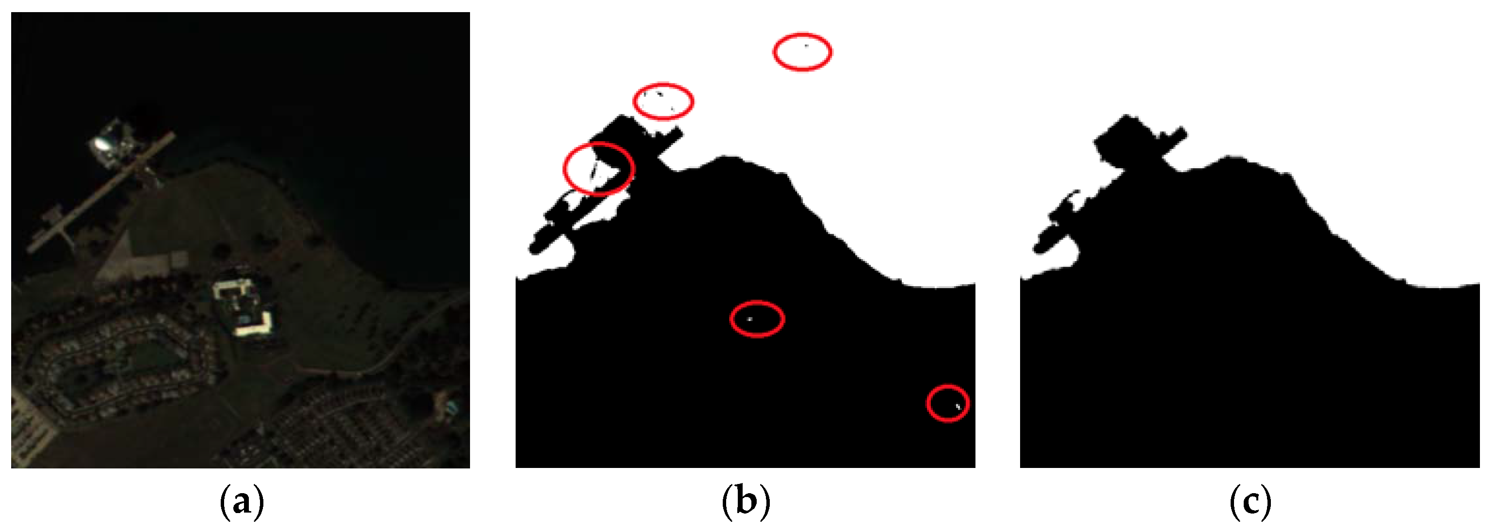
Figure 3.
Land-sea segmentation result of the sea covered by thick clouds. (a) The original image; and (b) the result of land-sea segmentation.
Figure 3.
Land-sea segmentation result of the sea covered by thick clouds. (a) The original image; and (b) the result of land-sea segmentation.
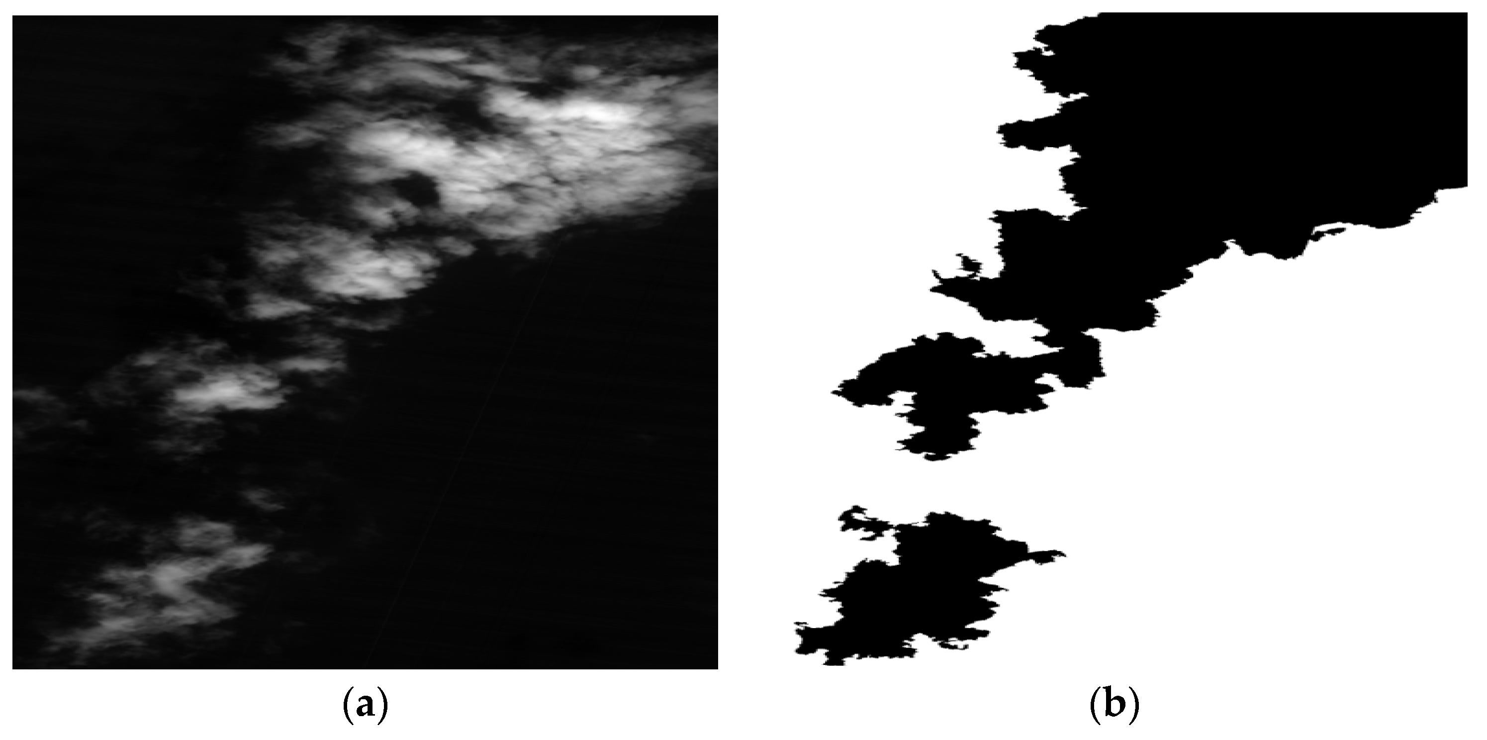
Figure 4.
A flowchart of the EWT.

Figure 5.
The result of localization of ROI based on PSMEWT. (a) The original image; (b) the phase significant map; (c) the binary image after adaptive dynamic threshold method; and (d) the localization of the ROI.
Figure 5.
The result of localization of ROI based on PSMEWT. (a) The original image; (b) the phase significant map; (c) the binary image after adaptive dynamic threshold method; and (d) the localization of the ROI.

Figure 6.
Comparison between DWT and EWT. (a) The original image; (b) horizontal high frequency component of DWT; (c) vertical high frequency component of DWT; (d) horizontal high frequency component of EWT; (e) vertical high frequency component of EWT; (f) multiplication of the high-frequency coefficients.
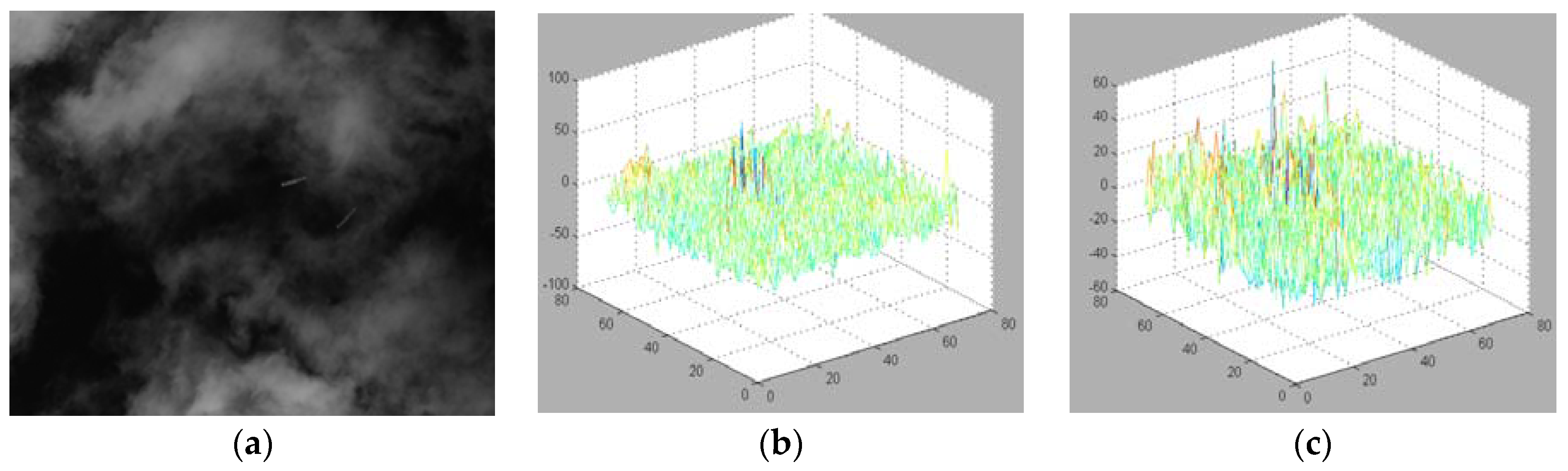

Figure 7.
The original images to be tested. (a) Strong waves; (b) cloud coverage.

Figure 8.
The localization results by Otsu. (a) The results of strong waves; (b) the results of cloud coverage.
Figure 8.
The localization results by Otsu. (a) The results of strong waves; (b) the results of cloud coverage.
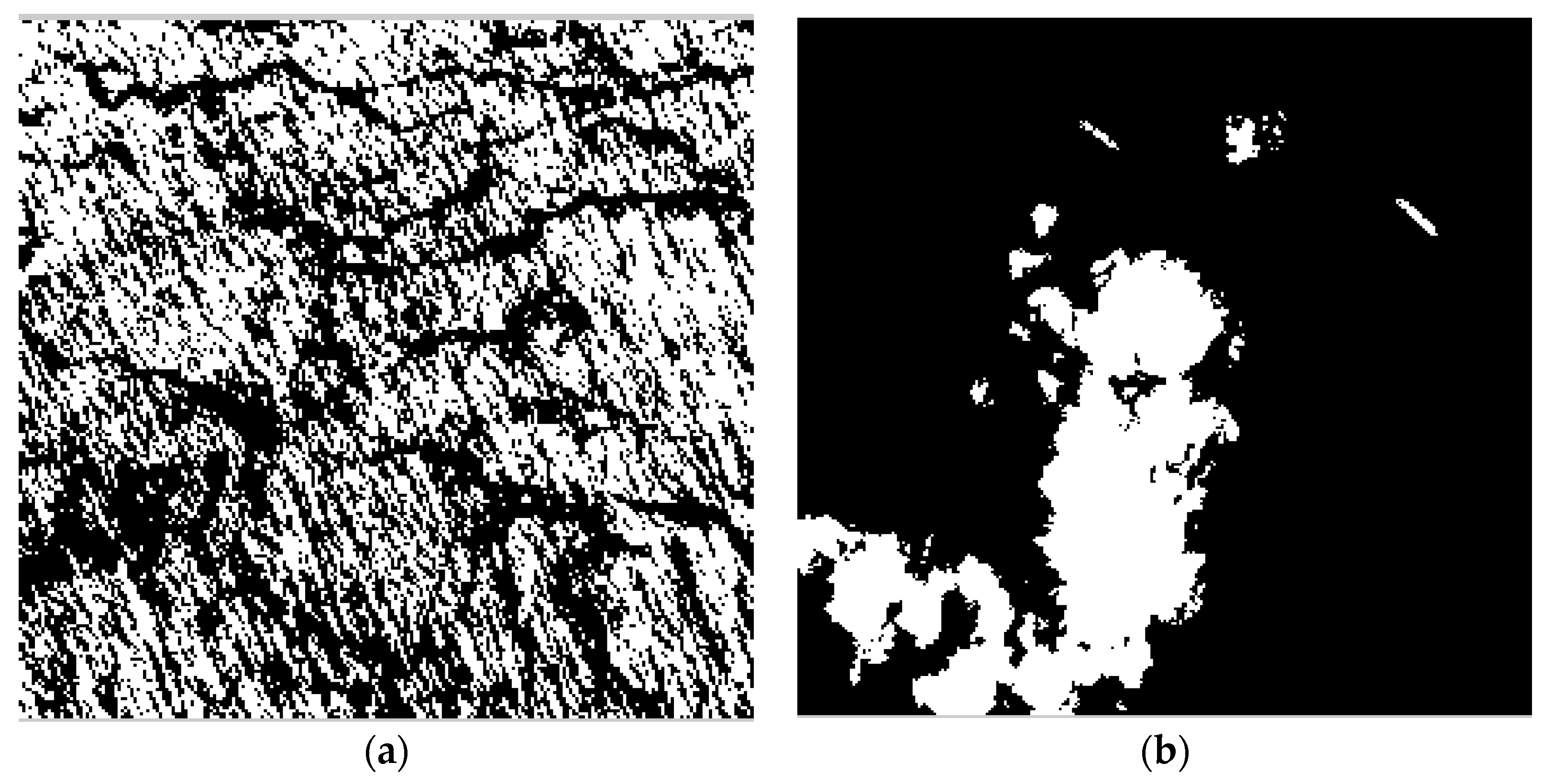
Figure 9.
The localization results by Canny. (a) The results of strong waves; (b) the results of cloud coverage.
Figure 9.
The localization results by Canny. (a) The results of strong waves; (b) the results of cloud coverage.

Figure 10.
The localization results of strong waves by PSMEWT. (a) The three-dimensional display of PSMEWT; (b) the localization results of PSMEWT.
Figure 10.
The localization results of strong waves by PSMEWT. (a) The three-dimensional display of PSMEWT; (b) the localization results of PSMEWT.
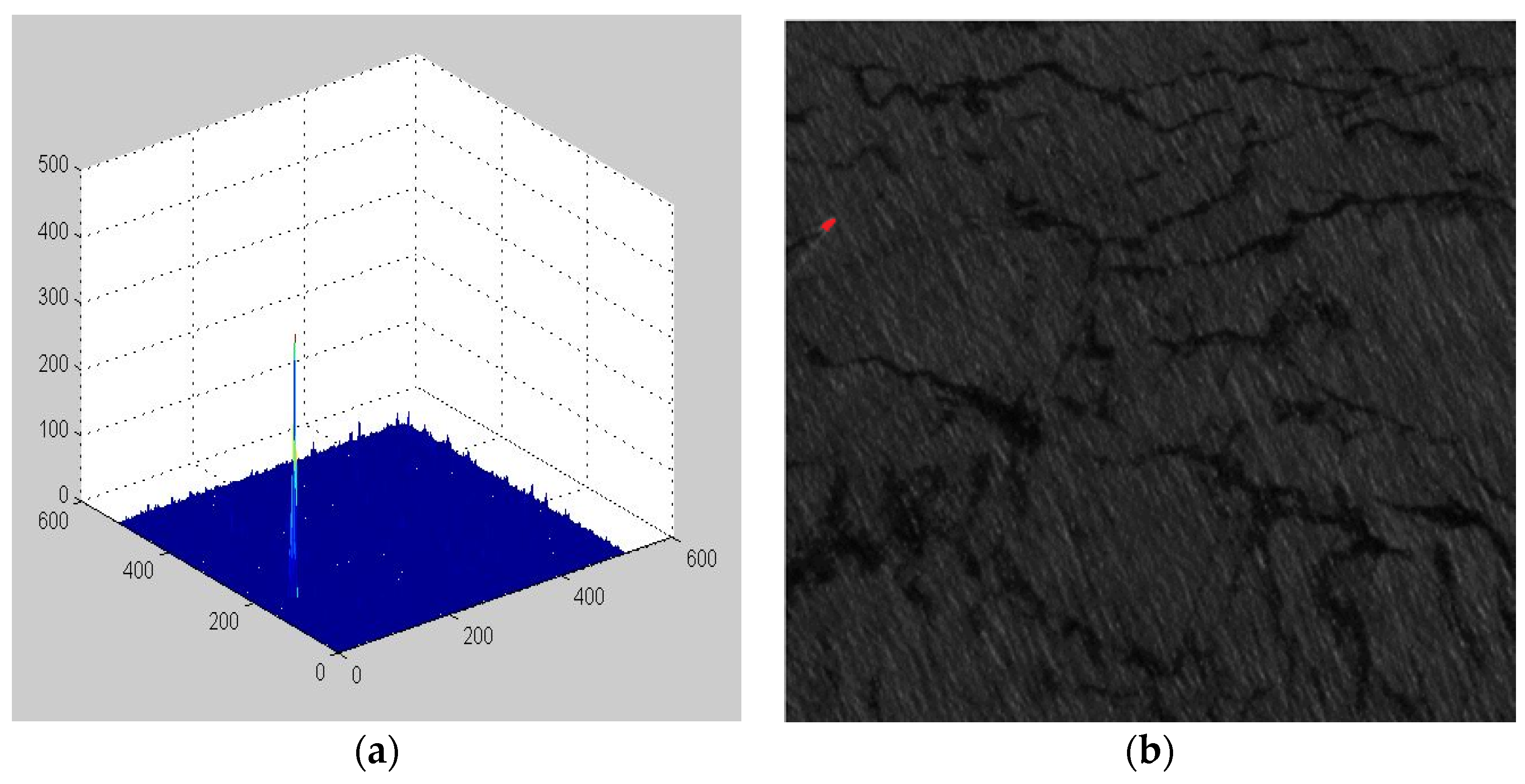
Figure 11.
The localization results of cloud coverage by PSMEWT. (a) The three-dimensional display of PSMEWT; (b) the localization results of PSMEWT.
Figure 11.
The localization results of cloud coverage by PSMEWT. (a) The three-dimensional display of PSMEWT; (b) the localization results of PSMEWT.

Figure 12.
The flowchart of the support vector machine (SVM) training process.

Figure 13.
Some sample slices. (a) Positive samples; and (b) some typical negative samples.
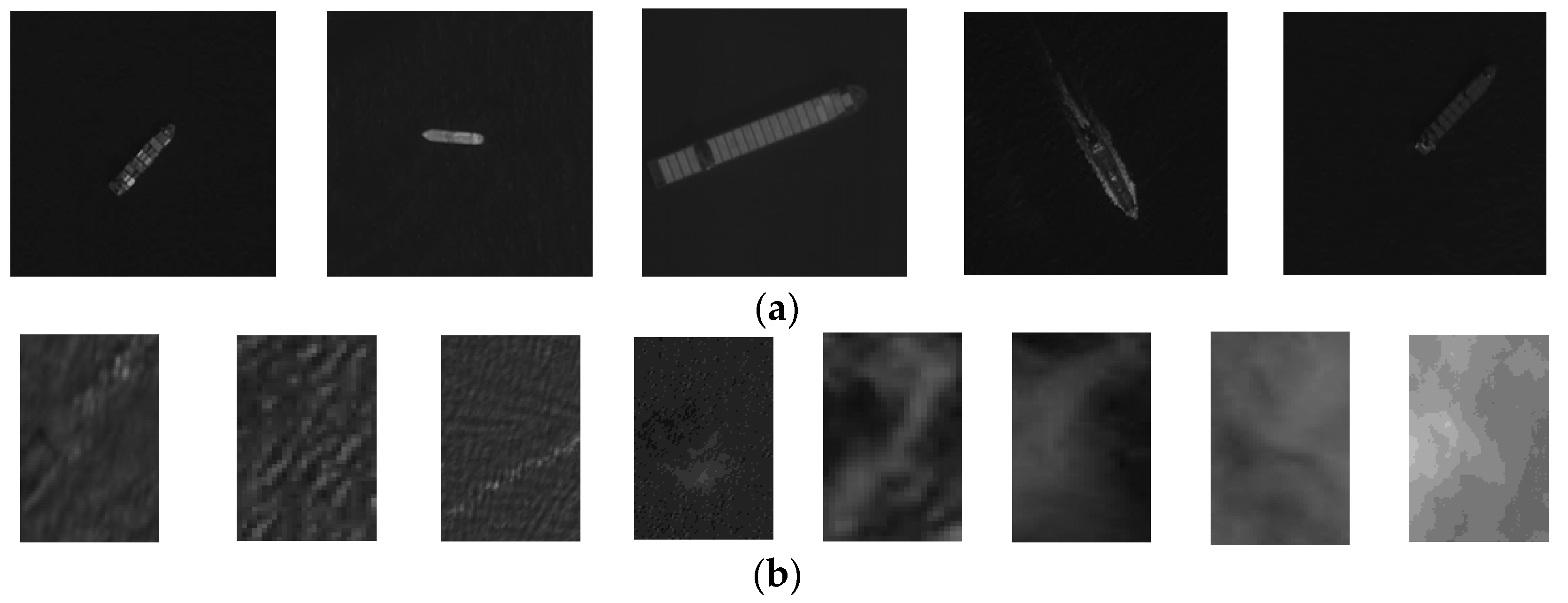
Figure 14.
The results of the feature statistical experiment. (a) The histogram variance of ; and (b) the correlation of GLCM.
Figure 14.
The results of the feature statistical experiment. (a) The histogram variance of ; and (b) the correlation of GLCM.
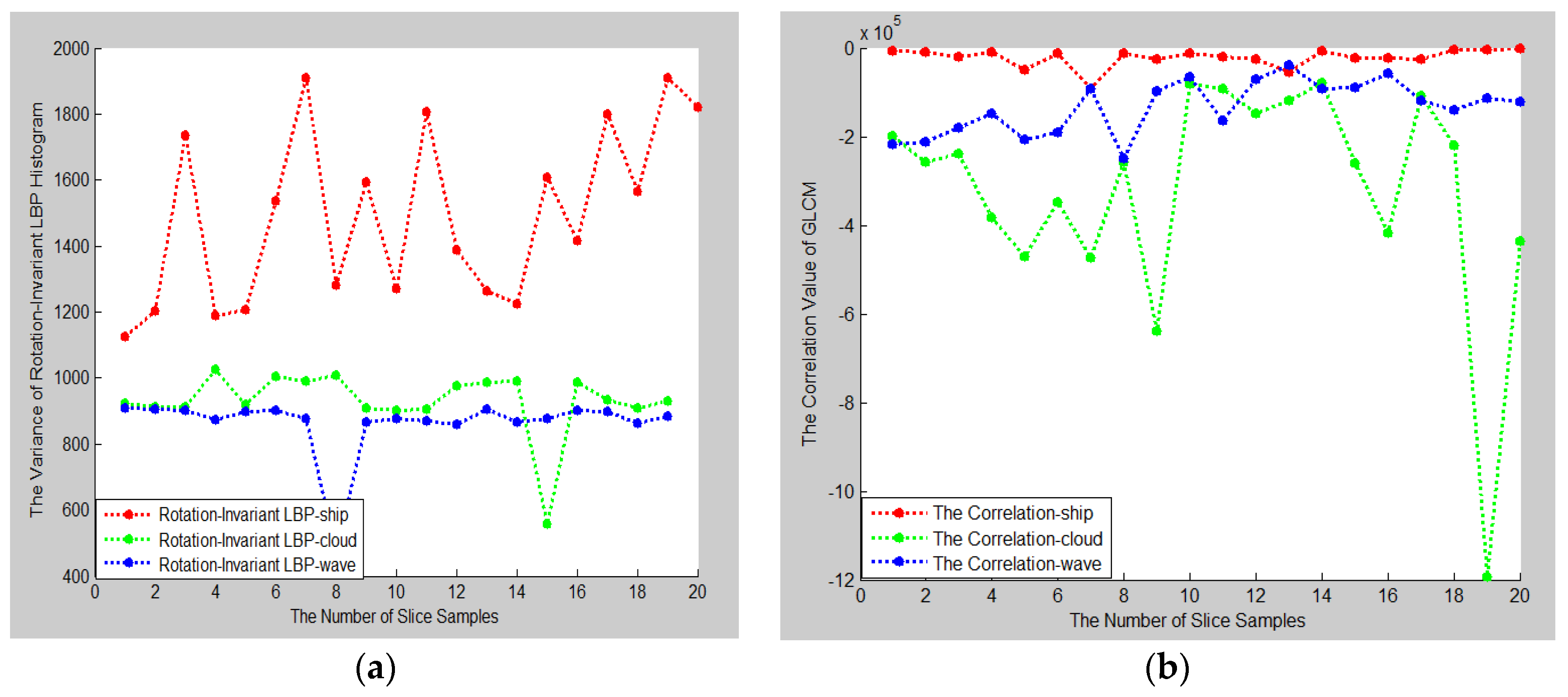
Figure 15.
The ship detection results from the three different methods. (a) An image covered by thin clouds; (b) the three-dimensional map of horizontal transformation coefficients by EWT; (c) the three-dimensional map of vertical transformation coefficients by EWT; (d) the final results of the EWT; (e) a binary segmentation image of phase significant map; (f) the detection results from our proposed method; (g) the detection results by the method in Reference [18]; (h) the detection results by the method in Reference [17].

Figure 16.
Examples of different sea surfaces. (a) Cloud coverage; (b) visible swell; (c) low contrast; and (d) simple sea.
Figure 16.
Examples of different sea surfaces. (a) Cloud coverage; (b) visible swell; (c) low contrast; and (d) simple sea.
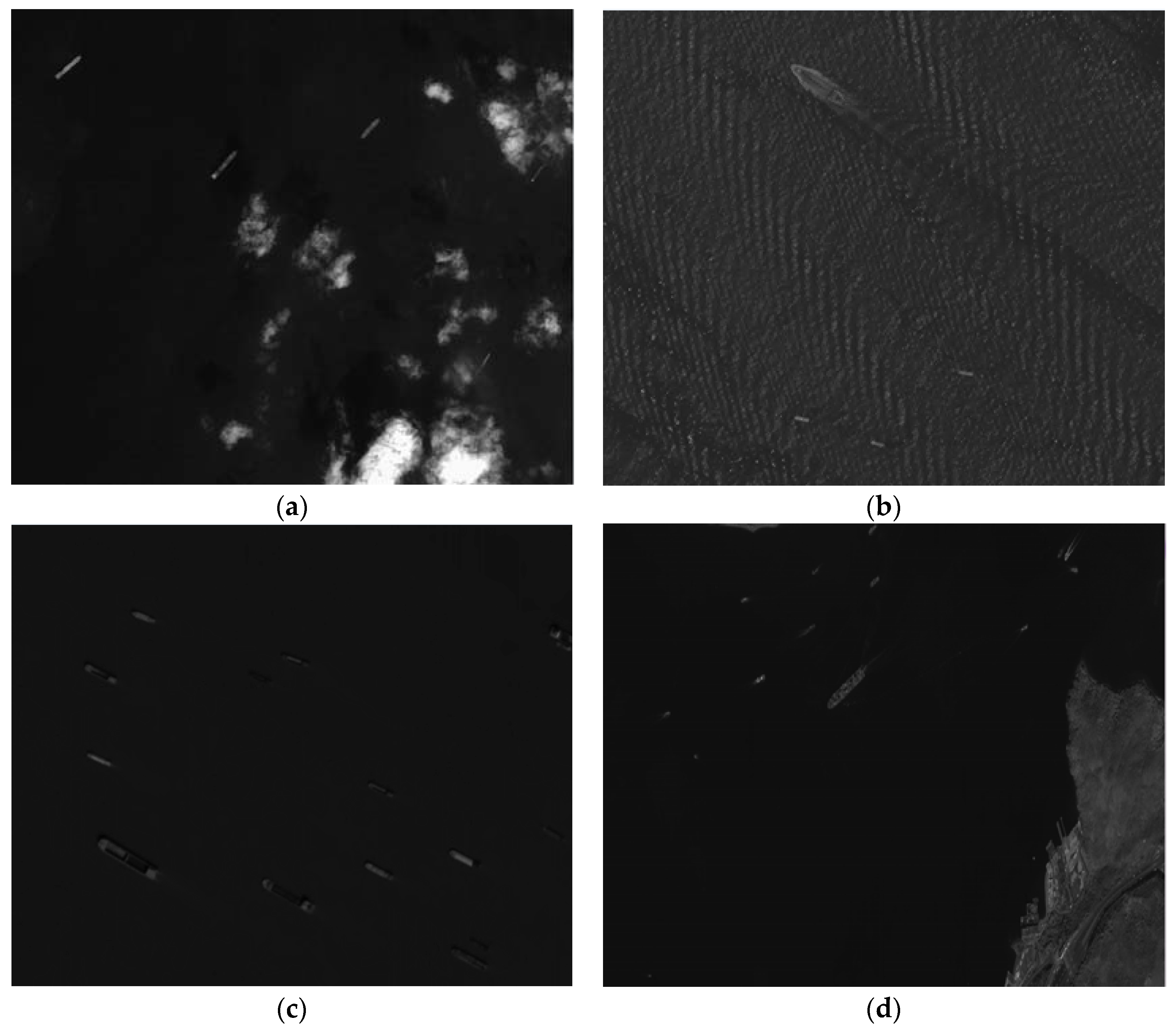
Figure 17.
The binary significant images after PSMEWT. (a) Cloud coverage; (b) visible swell; (c) low contrast; and (d) simple sea.
Figure 17.
The binary significant images after PSMEWT. (a) Cloud coverage; (b) visible swell; (c) low contrast; and (d) simple sea.
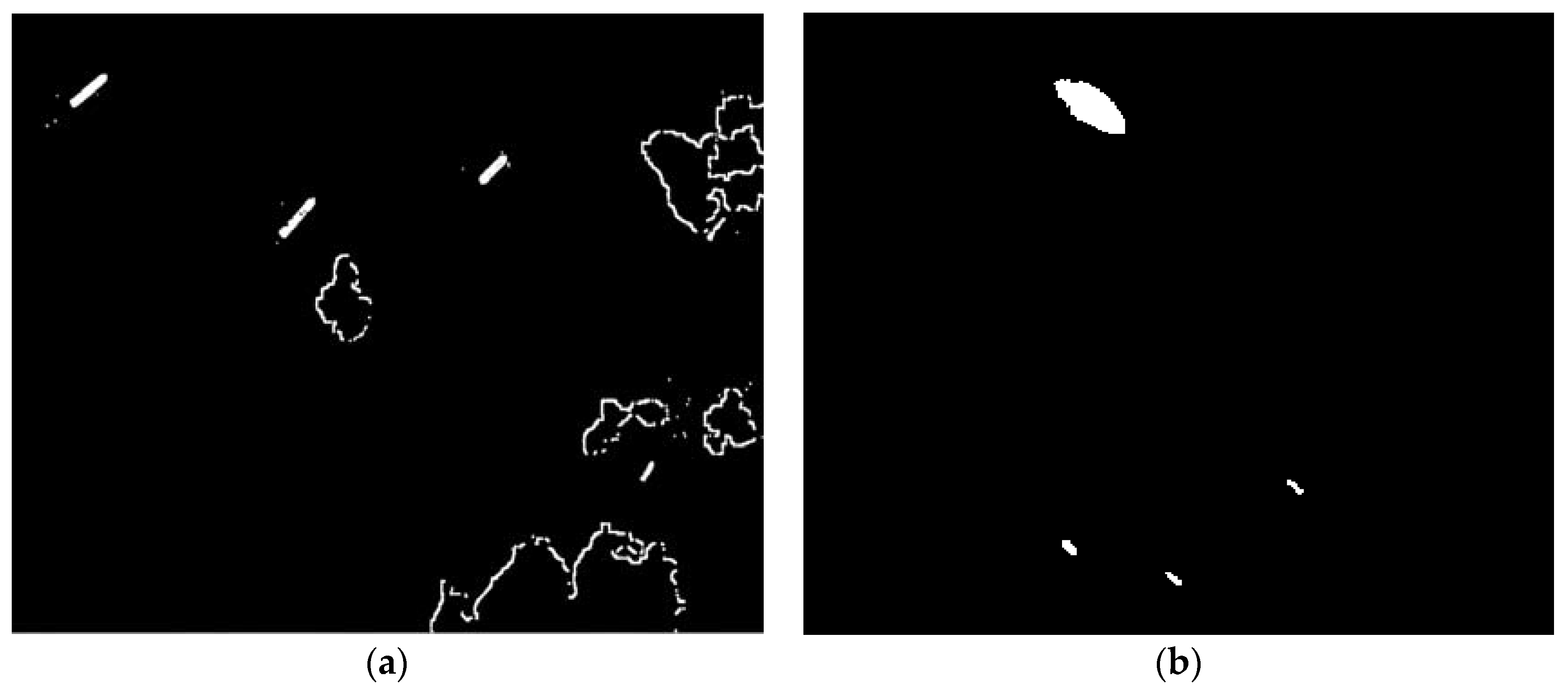

Figure 18.
The detected ships. (a) Cloud coverage; (b) visible swell; (c) low contrast; and (d) simple sea.
Figure 18.
The detected ships. (a) Cloud coverage; (b) visible swell; (c) low contrast; and (d) simple sea.


Table 1.
Detection results of our method in various situations.
| Different Situations | Recall | Precision |
|---|---|---|
| Quiet sea | 97.74% | 96.30% |
| Textured sea | 91.61% | 86.75% |
| Clutter sea | 82.05% | 71.11% |
© 2017 by the authors. Licensee MDPI, Basel, Switzerland. This article is an open access article distributed under the terms and conditions of the Creative Commons Attribution (CC BY) license (http://creativecommons.org/licenses/by/4.0/).
Share and Cite
MDPI and ACS Style
Nie, T.; He, B.; Bi, G.; Zhang, Y.; Wang, W. A Method of Ship Detection under Complex Background. ISPRS Int. J. Geo-Inf. 2017, 6, 159. https://doi.org/10.3390/ijgi6060159
AMA Style
Nie T, He B, Bi G, Zhang Y, Wang W. A Method of Ship Detection under Complex Background. ISPRS International Journal of Geo-Information. 2017; 6(6):159. https://doi.org/10.3390/ijgi6060159
Chicago/Turabian StyleNie, Ting, Bin He, Guoling Bi, Yu Zhang, and Wensheng Wang. 2017. "A Method of Ship Detection under Complex Background" ISPRS International Journal of Geo-Information 6, no. 6: 159. https://doi.org/10.3390/ijgi6060159
Note that from the first issue of 2016, this journal uses article numbers instead of page numbers. See further details here.