The Relationship between an Invasive Shrub and Soil Moisture: Seasonal Interactions and Spatially Covarying Relations

Abstract

Recent studies indicate that positive relationships between invasive plants and soil can contribute to further plant invasions. However, it remains unclear whether these relations remain unchanged throughout the growing season. In this study, spatial sequences of field observations along a transect were used to reveal seasonal interactions and spatially covarying relations between one common invasive shrub (Tartarian Honeysuckle, Lonicera tatarica) and soil moisture in a tall grassland habitat. Statistical analysis over the transect shows that the contrast between soil moisture in shrub and herbaceous patches vary with season and precipitation. Overall, a negatively covarying relationship between shrub and soil moisture (i.e., drier surface soils at shrub microsites) exists during the very early growing period (e.g., May), while in summer a positively covarying phenomenon (i.e., wetter soils under shrubs) is usually evident, but could be weakened or vanish during long precipitation-free periods. If there is sufficient rainfall, surface soil moisture and leaf area index (LAI) often spatially covary with significant spatial oscillations at an invariant scale (which is governed by the shrub spatial pattern and is about 8 m), but their phase relation in space varies with season, consistent with the seasonal variability of the co-varying phenomena between shrub invasion and soil water content. The findings are important for establishing more complete picture of how shrub invasion affects soil moisture.

1. Introduction

Shrub encroachment into managed or natural ecosystems has been recognized as a global phenomenon with multiple biogeochemical and socio-economic consequences [1,2,3,4,5,6]. The Tartarian Honeysuckle (Lonicera tatarica) is one of the most aggressive shrub species in North America and poses a serious threat to managed and natural ecosystems [7,8,9]. Tartarian Honeysuckle is a woody shrub which was introduced into North American from Central Asia in 1752 as a landscape plant because of its early spring flowers and numerous attractive red berries. Tartarian honeysuckle can spread rapidly through faunal mechanisms of seed dispersal and is capable of forming a dense canopy which restricts native plant growth [9]. The species can be commonly found in old fields, floodplains, forest edges and roadsides in the central and eastern Ontario, Canada and throughout eastern and central United States [9]. The woody plants, shrubs, and invasive shrubs mentioned hereafter are all referring to Tartarian honeysuckle.

Studies investigating ecosystem or community responses to plant invasion have increased our understanding of the invasion process. Recent studies have indicated positive relationships between invasive plants and soil properties which promote further plant invasions [10,11,12]. Among soil properties that influence plant species composition, soil moisture balance is the most important factor that determines vegetation spatial distribution [13]. Over the last few decades, the relations between woody plants and soil moisture have been discussed largely by comparing a time series of soil moisture observations beneath woody plant canopy to an adjacent intercanopy/grass patch [14,15,16,17,18]. In general, there has been a lack of studies using spatial sequences (i.e., a spatial series of data points measured typically at successive locations in space at uniform intervals) of measurements to evaluate the effects of canopy cover on soil water content.

An accurate understanding of the association between Tartarian honeysuckle and soil water content over time and space is crucial to evaluating the effects of shrub invasion on soil resources available to native grasses. Soil moisture typically shows considerable variability across a range of scales in space and time. Large-scale spatial and temporal variations in soil moisture are driven largely by meteorological conditions [19]. At smaller scales, soil moisture is often subject to the effects of numerous environmental factors, such as soil type, landscape position, vegetation, and topography [20]. Studies have suggested that woody plants could substantially affect soil water content in time and space via multiple mechanisms [14,15,16,17,18,21]. On one hand, the establishment and expansion of woody species relies on soil water availability [22]. The growth, transpiration, and interception of vegetation canopies could decrease water storage in the soils beneath plant canopies. On the other hand, canopy shading could lead to a reduction in evaporative losses and therefore enhance subcanopy soil water content [14,17,21]. In addition, woody plants could also trigger higher soil moisture through intensified soil infiltration [23]. Thus, one might expect variable interactions between woody plants and underlying soil moisture. Therefore, the major hypothesis underlying this research is that there are causality links between Tartarian honeysuckle and soil moisture across space and these causality links vary in a predictable manner in response to the establishment of shrubs and microclimate conditions.

The objective of this study was to identify the shrub-soil moisture covarying relations in space and the relevant temporal variability. Field observations along a transect in a common old field habitat, which is characterized by a mixture of native herbaceous species and a highly invasive shrub Tartarian Honeysuckle, were used to reveal the relationship between the shrub and underlying soil moisture. The old field was selected for this analysis because (1) it represents one of the typical habitats invaded by the Tartarian honeysuckle [9] and (2) the flat topography and well-drained/uniformly graded sandy loam soil ensures that the observed differences are not a product of unmeasured environmental variations.

2. Methodology

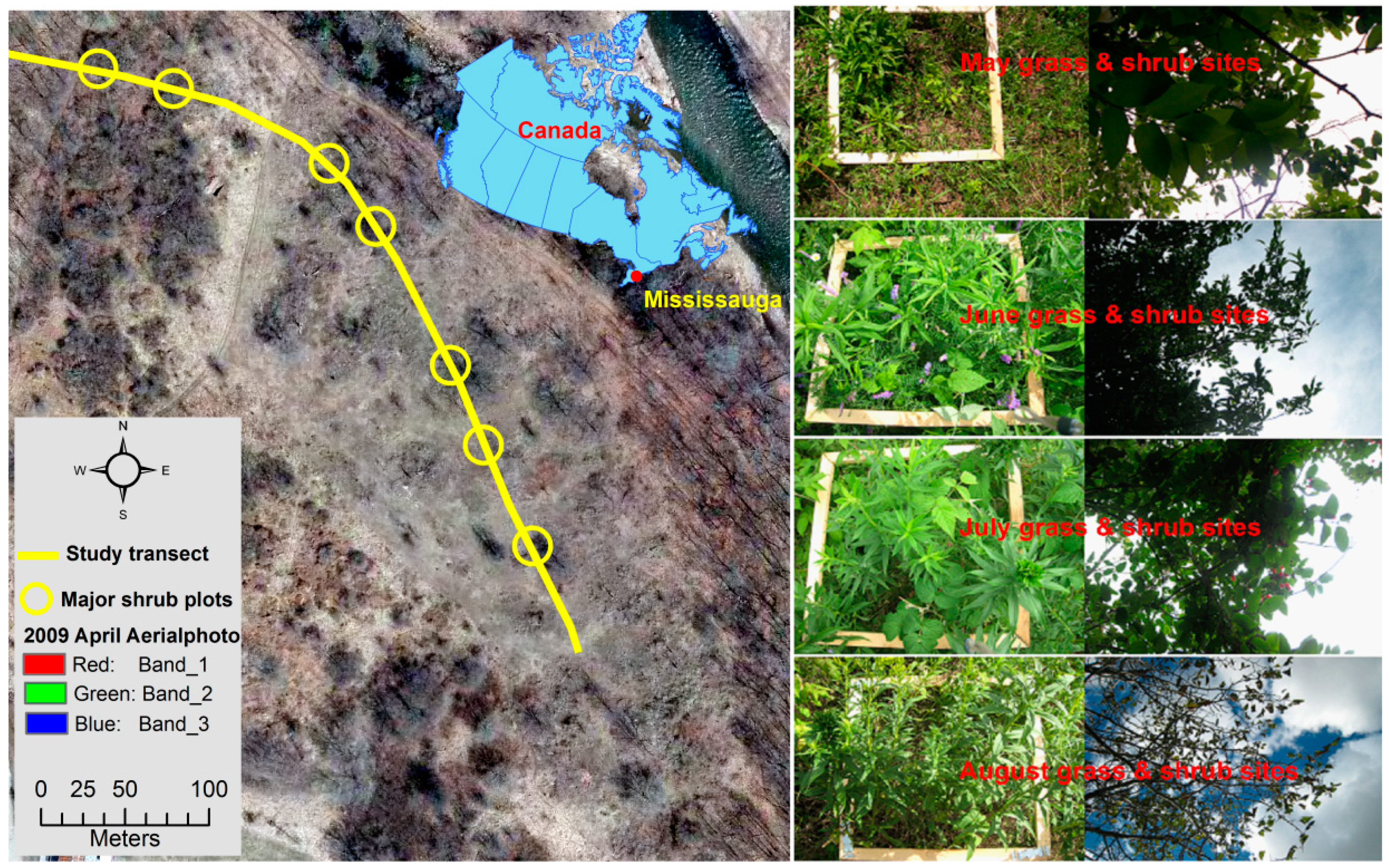
2.1. Study Area and Data Collection

The study was conducted in an old field habitat located at the University of Toronto Mississauga (UTM), Ontario, Canada (43.55°N, 79.66°W) (Figure 1). The study area is 3.5 hectares in size and has been undisturbed for at least 80 years with no formal entrance and crosswalk. The area has a flat terrain with well-trained and uniformly graded sandy loam soil. The field is dominated by herbaceous species, such as Orchard Grass (Dactylis glomerata), Kentucky Bluegrass (Poa pratensis), Goldenrod (Solidago) and Purple Milkweed (Asclepias purpurascens), but is also heavily invaded by the Tartarian Honeysuckle shrub. As mapped by aerial photographs, the Tartarian Honeysuckle only occupied 2% of the study area in 1983 but increased to 25% in 2005.

Figure 1. Map indicating the study area, the study transect (the yellow line), the large shrub patches in yellow circle, and field photos taken from an herbaceous macrosite and a shrub macrosite at four observation times.

Figure 1. Map indicating the study area, the study transect (the yellow line), the large shrub patches in yellow circle, and field photos taken from an herbaceous macrosite and a shrub macrosite at four observation times.

Field observations along the transect (2 m spacing, 128 sampling microsites) were conducted four times during the 2010 growing season (10–11 May, 21–22 June, 15–17 July, and 20–21 August 2010). At each sampling microsite, leaf area index (LAI), surface soil moisture, and species composition data were collected within a quadrat of 50 cm × 50 cm. LAI was measured using an AccuPAR LP-80 Ceptometer. Soil volumetric water content (VWC; top 12 cm) was measured using a HydroSense 620 Water Content Sensor (five measurements per 50 cm × 50 cm quadrat). Here, based upon the collected species composition data, a sampling point is referred to as a shrub patch if the shrub coverage exceeded 50% (within 50 cm × 50 cm quadrat), otherwise it is categorized as an herbaceous patch. The percent shrub coverage per plot was quantified through field hemispherical photography using a software package called CAN-EYE [24]. All the measurements were made at least 2–3 days after any environmental events (e.g., rainfall) to ensure the stability of the data. The corresponding precipitation data are publicly available in the Department of Geography, University of Toronto [25].

2.2. Data Analysis

Wavelet analysis including the Morlet continuous wavelet transform and wavelet coherence was used in this study to examine the spatial connection between LAI and soil moisture spatial series in light of the expected causality links between shrubs and soil moisture across space. Wavelet analysis is becoming an increasingly common tool for analyzing spatial data owing to its capability to provide both a local evaluation of spatial structure and a global analysis of spatial pattern along the transect. One way to interpret wavelet analysis is through use of the wavelet as a scalable windowing function, which describes a template that can be scaled to a desired size and then slid along the transect [26,27]. The wavelet power is high when the template fits the observed data well. Many possible wavelet functions are available to choose for an analysis [28,29,30]. The author used the Morlet wavelet function in this study because it has been shown to provide a good balance between space and frequency localization [31,32,33,34]. Continuous wavelet transform was performed since it is a suitable tool for analyzing localized intermittent oscillations in a spatial series [35].

Based upon the method described in Torrence and Webster [35] and Grinsted et al. [31], the Morlet continuous wavelet transform (with dimensionless frequency = 6) was first applied to identify dominant spatial scales (i.e., the width of the wavelet) at which the spatial sequence of LAI or soil moisture would show a periodic spatial pattern. In order to separate true periodic spatial patterns at certain scale from random fluctuations, the statistical significance of wavelet power was estimated against a red noise model for each spatial series. Following this, the wavelet coherence (the square of the cross-spectrum normalized by the individual power spectra) and phase angle was computed to identify co-varying relationships between the localized signals from the spatial series of the two variables (i.e., LAI and soil moisture). One can picture wavelet coherence as a correlation coefficient: Ranging from 0–1 and the closer the value to 1 indicates the more correlated the two series are. Similarly, the phase angle, shown as arrows in the coherence spectra, is similar to the sign of a correlation coefficient. If the coherence between LAI and soil moisture along the transect is high, the phase angle at 0° (arrows pointing to horizontal right) implies an in-phase linear coherence while the phase angle at 180° (horizontal left) indicating an anti-phase linear coherence. Non-horizontal arrows indicate an out of phase situation, meaning that the two series at that location do not have a linear relation but a more complex relationship. The 5% statistical significance level of the wavelet coherence against red noise was estimated using Monte Carlo methods. The wavelet coherence calculations were completed using the software provided by A. Grinsted [36]. Significance of wavelet power and coherence was assessed following the procedures in Grinsted et al. [31].

According to the sampling theorem [37], an optimum sampling length is approximately one-fourth of the significant scale identified by the wavelet analysis. Therefore, a sampling interval of 2 m used in this study is sufficient to capture an 8-m covarying pattern between shrubs and soil moisture. However, any co-varying patterns at a scale less than 8 m would not be caught because data less than 2 m were not sampled. The author would like to clarify that the 2-m sampling interval has no negative impact to the results of this study because vegetation coverage within 2-m intervals is very uniform in the area and thus LAI and soil moisture collected within 2 m are sufficient for the identification of their spatial patterns. An interval less than 2 m would be recommended if the focus of the study is to identify vegetation process at the species level.

3. Results and Discussion

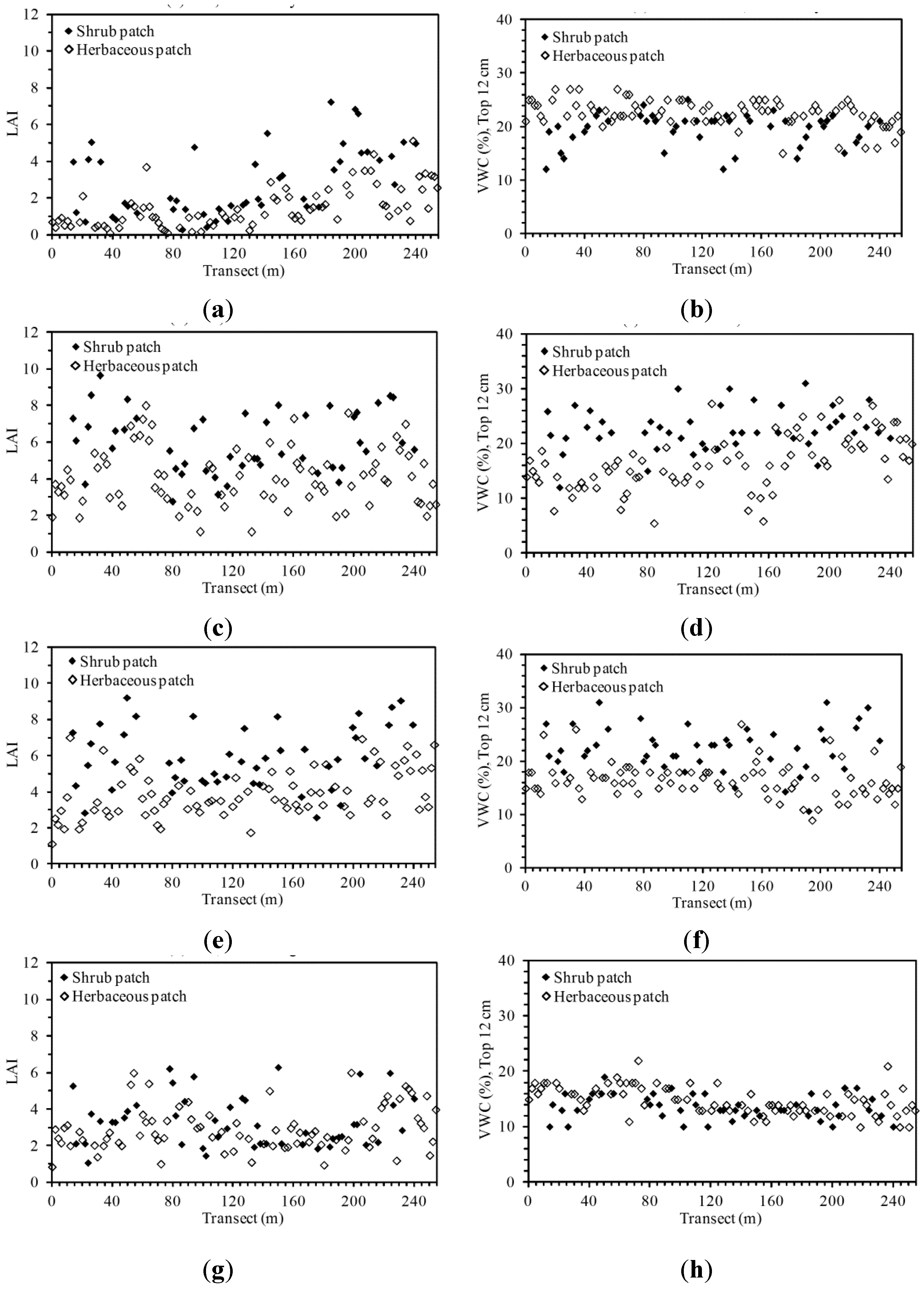
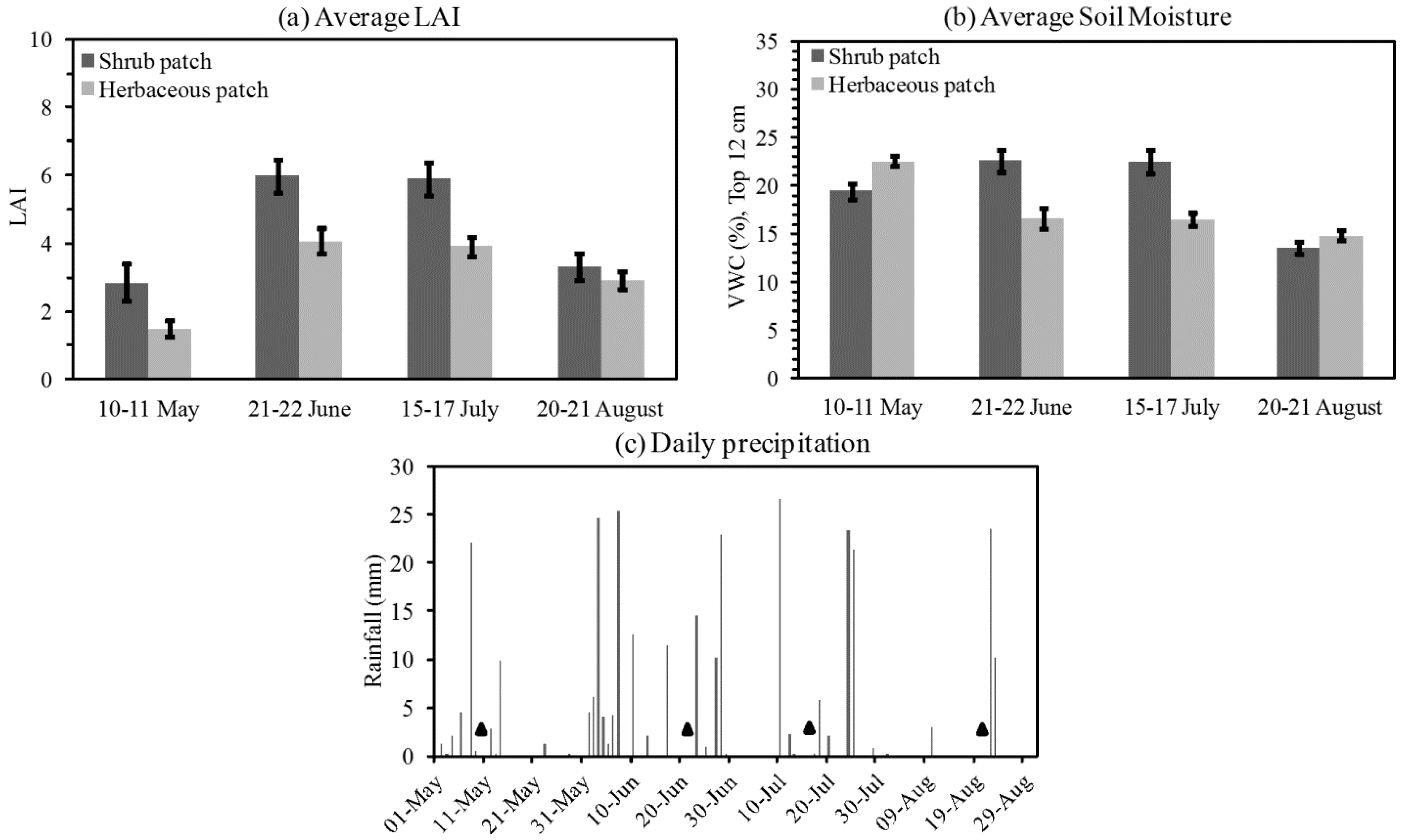
3.1. Descriptive Analysis of LAI and VWC Sequences

Figure 2 shows the sequences of LAI and VWC along the study transect at four observation times (10–11 May, 21–22 June, 15–17 July, and 20–21 August 2010). The average values of all shrub patches and of all herbaceous patches are plotted in Figure 3a (LAI) and Figure 3b (VWC). As illustrated in Figure 2 and Figure 3, both LAI and surface soil moisture measurements show evident differences between shrub and herbaceous microsites. These differences vary with the observation time. As observed on 10–11 May, the shrub patches show higher LAI overall (Figure 2a and Figure 3a), but have drier surface soils (Figure 2b and Figure 3b) than herbaceous microsites. Differences in transect-averaged LAI and VWC values between shrub and herbaceous microsites are statistically significant (Figure 3a,b). Figure 3c provides the daily precipitation amounts at this study site during May–August 2010. In early May, soil water is plentiful due to frequent rainfall events (Figure 3c). Moving to the 21–22 June and 15–17 July measurements, LAI witnesses a considerable increase at almost all the sampling microsites (Figure 2c,e). This is consistent with increased available soil water because of more frequent and stronger precipitation events (Figure 3b). Transect-averaged LAI at shrub microsites is significantly higher than in herbaceous patches (Figure 3a). In contrast to the 10–11 May measurement, however, wetter surface soils are observed at shrub locations on 21–22 June and 15–17 July (Figure 2d,f). Average VWC (top 12 cm) of all shrub patches along the transect is about 6% higher than that of all herbaceous microsites at these two observation times (Figure 3b). The LAI values observed on 20–21 August (Figure 2g) are, relative to those in June–July (Figure 2c,e), considerably decreased, especially at shrub microsites (Figure 3a). This may be due to the fact that shrubs lose their leaves in response to a long dry period (Figure 3c). The differences in transect-averaged LAI and VWC between shrub and herbaceous locations are marginal and are not statistically significant (<95% level) for the 20–21 August measurement (Figure 3a,b).

The results presented in Figure 2 and Figure 3 reveal seasonal variability between surface soil moisture values at shrub and herbaceous microsites (i.e., drier surface soils at shrub microsites on 10–11 May, wetter shrub soils on 21–22 June and 15–17 July, and comparable VWC for the 20–21 August measurement). The author believes that this is an indication of a covarying relationship between shrubs and soil moisture, which is explained as follows. In the early growing months (e.g., April–May), the averaged soil moisture level over the transect is governed mainly by precipitation (and snow melting if snow exists) since soil evaporation is relatively weak due to moderate insolation and air/surface temperatures. There are frequent rainfall events in early May 2010 (Figure 3c). Accordingly, the mean soil moisture level (including both shrub and herbaceous patches) is high for the 10–11 May measurement (Figure 3b). At that observation time, the soil water losses because of evaporation were small and comparable between shrub and herbaceous microsites, while more soil water could be consumed in shrub patches due to the competition between shrubs and herbaceous species. This may reflect a negative impact of shrubs on surface soil moisture.

Figure 2. Spatial sequences of leaf area index (LAI) and soil volumetric water content (VWC, top 12 cm) along the transect at four observation times (a,b) LAI and VWC on 10–11 May, (c,d) LAI and VWC on 21–22 June, (e,f) LAI and VWC on 15–17 July, and (g,h) LAI and VWC on 20–21 August 2010). Black solid (unfilled) diamond represents shrub (herbaceous) microsite.

Figure 2. Spatial sequences of leaf area index (LAI) and soil volumetric water content (VWC, top 12 cm) along the transect at four observation times (a,b) LAI and VWC on 10–11 May, (c,d) LAI and VWC on 21–22 June, (e,f) LAI and VWC on 15–17 July, and (g,h) LAI and VWC on 20–21 August 2010). Black solid (unfilled) diamond represents shrub (herbaceous) microsite.

Figure 3. (a) Average LAI of all shrub patches (black bars) and of all herbaceous patches (grey bars) along the transect at four observation times (from left to right: 10–11 May, 21–22 June, 15–17 July, and 20–21 August 2010). The error bars indicate 95% confidence intervals; (b) Similar to (a), but for soil volumetric water content (VWC, top 12 cm); (c) Daily precipitation amounts at this site during May–August 2010; Triangles in panel (c) indicate the four observation times in panels (a) and (b).

Figure 3. (a) Average LAI of all shrub patches (black bars) and of all herbaceous patches (grey bars) along the transect at four observation times (from left to right: 10–11 May, 21–22 June, 15–17 July, and 20–21 August 2010). The error bars indicate 95% confidence intervals; (b) Similar to (a), but for soil volumetric water content (VWC, top 12 cm); (c) Daily precipitation amounts at this site during May–August 2010; Triangles in panel (c) indicate the four observation times in panels (a) and (b).

Turning to the peak growing period (June to September), the evaporative losses are likely to become considerable due to strong solar irradiance and therefore soil moisture in open areas is substantially affected by both precipitation and soil evaporation. In months with frequent rainfall events (e.g., June and July 2010; Figure 3c), the shrubs can grow rapidly with dense canopy coverage, as indicated by very high LAI values at shrub microsites (Figure 2c,e, and Figure 3a). Although the growth and transpiration of shrubs, relative to herbaceous species, may require more soil water, the evaporative losses are less significant beneath shrubs than in herbaceous patches since shading formed by the very dense shrub cover could lead to a substantial reduction in surface evaporation. Thus, the net effect could be that the surface soils at shrub microsites stay relatively wet, likely indicating a positive shrub-soil moisture relation. D’Odorico et al. [14] showed a positive relationship between surface soil moisture (top 10 cm) and tree canopy cover at the moist end of the Kalahari Transect over the local wet season. In the study, the shading effect was also proposed as the key mechanism for the wetter soils under canopies, i.e., soil wetness beneath canopies can be conserved by canopy shading (through low evaporative losses), which could offset or even overcome the effects of the canopy interception/transpiration on soil water losses [21].

When a long dry period occurs during the peak growing season (e.g., in August 2010; Figure 3c), shrubs lose their leaves and their ability to create dense shading as indicated by the small LAI in shrub patches during this period (Figure 2g and Figure 3a). Accordingly, the evaporative losses at shrub microsites may be considerably increased and become comparable to those at herbaceous sites [38]. As a result, the significant difference in soil moisture between shrub and herbaceous spaces may diminish or even vanish due to reductions in shrub canopy after a long dry period (Figure 2h and Figure 3b), thus leading to a weak interaction between shrub and VWC. This further supports the hypothesis that shading by shrub canopies plays a critical role in yielding a positive relationship between shrubs and soil moisture as observed in June and July. If new precipitation events (or irrigation) occur following a long rainless spell, the dense coverage of shrub canopy [39] and its resultant association to increased soil moisture could be recovered. In a common habitat, other land parameters, such as topography and soil type, are expected to influence soil moisture comparably beneath shrub canopy and in herbaceous space. As their effects are small in this study, they can be considered negligible since the author is most interested in the contrast between shrub and herbaceous patches.

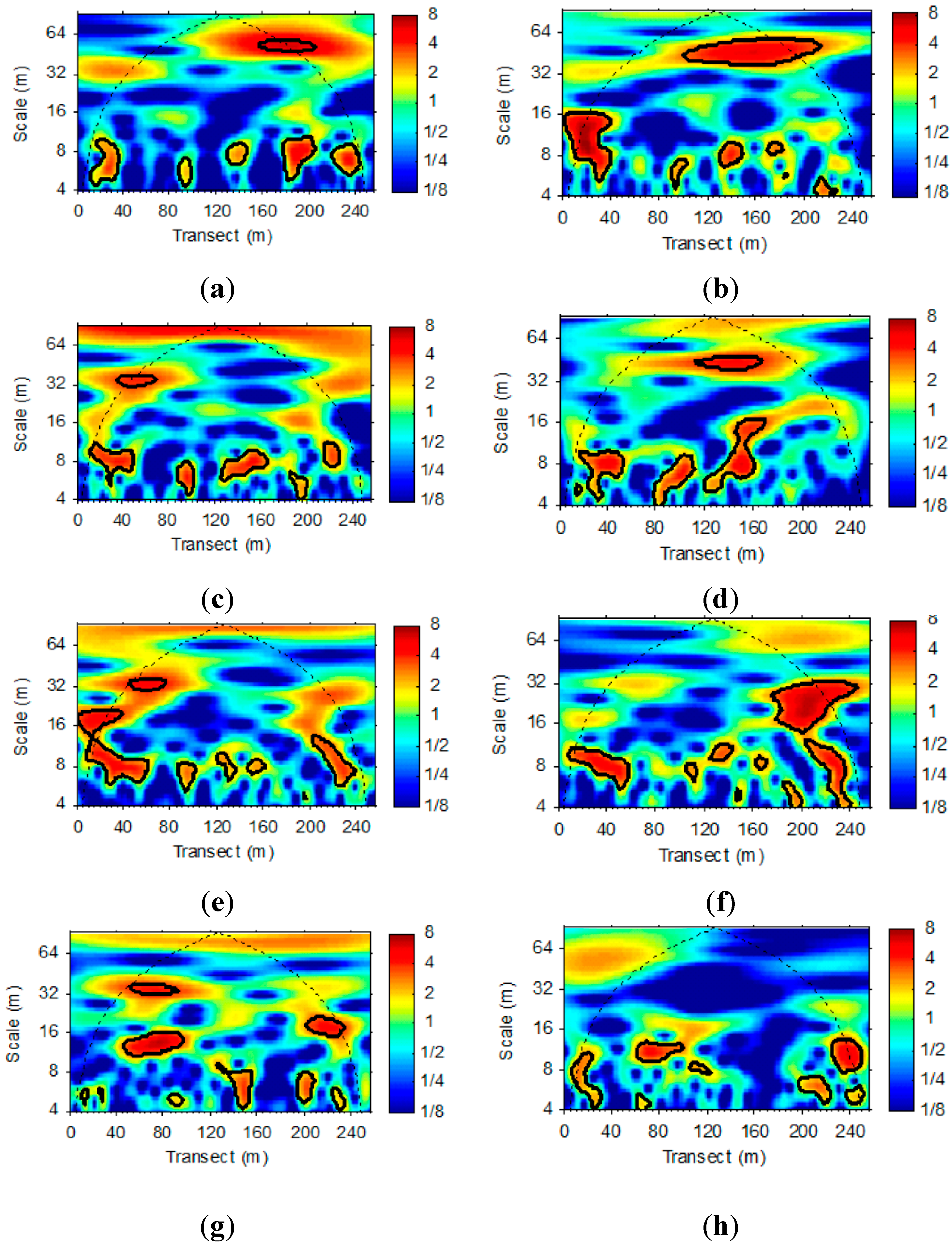
3.2. Wavelet Analysis of LAI and VWC Sequences

To further identify scales for significant spatial oscillations in the two spatial series, the wavelet power spectra of the LAI and VWC are calculated along the transect and the power (variance) ranges from weak (blue shades) to strong (red shades) in Figure 4. Except for the 20–21 August measurement, a common scale of 8-m variation is exhibited in both LAI and soil moisture spatial series across the season. In other words, high variances (yellow to red shades) at the 8-m scale are seen in the locations of 30 m, 95 m, 140 m, 180 m, and 220 m in both LAI (Figure 4a,c,e) and VWC (Figure 4b,d,f) sequences along the transect and these variances are significantly different from that of red noise (contour with solid black line). This result indicates that there is an overall positive agreement between LAI and VWC sequences with respect to the wavelet spectrum power pattern. Remotely sensed LAI data (acquired in mid-July 2009 and for the same study site) indicate a similar spatial scale [25]. At distances where the 8 m scale oscillations significantly occur (e.g., at 30 m, 95 m, and 140 m away from the origin of the transect; Figure 4a,c,e and b,d,f), the shrub-dominance can be seen (Figure 1) and the associated LAI and VWC anomalies thus also occur (i.e., larger LAI in May–July, lower VWC in May, and higher VWC in June and July; Figure 2a,c,e and b,d,f). This indicates that the occurrence of a pronounced 8-m spatial scale in LAI and soil moisture could be due to shrub invasion to herbaceous species. Other than an 8-m scale, the wavelet spectra are also strong at larger spatial scales, e.g., 16 m, 32 m and 64 m for LAI and VWC sampled in May–July (Figure 4a,c,e and b,d,f ), although the edge effects are often large at these scales and therefore no further discussion will be attempted.

The 20–21 August measurement does not show evident spatial oscillations at an 8-m scale in LAI and VWC (Figure 4g,h). Instead, significant wavelet power values (yellow to red shades within thick black contours) are seen only at smaller (between 4 and 6 m) or larger (between 10 and 16 m) scales (Figure 4g,h). At that observation time, as mentioned previously, the differences in LAI and VWC between shrub and herbaceous spaces are marginal and statistically insignificant (Figure 2g,h and Figure 3a,b). This may result in the absence of an evident 8-m scale in the 20–21 August measurement of LAI and VWC (Figure 4g,h).

Figure 4. Wavelet power spectrum of LAI and soil volumetric water content (VWC, top 12 cm) spatial sequences obtained at four observation times ((a,b) wavelet power spectrum of LAI and VWC on 10–11 May, (c,d) wavelet power spectrum of LAI and VWC on 21–22 June, (e,f) wavelet power spectrum of LAI and VWC on 15–17 July and (g,h) wavelet power spectrum of LAI and VWC on 20–21 August 2010). The wavelet power (colored shading) is normalized by 1/σ² (σ² represent the variance of each spatial sequence). The vertical axis represents the spatial scale of variation (i.e., the Fourier period), while the horizontal axis is the transect. The thick black contour indicates the 95% significance level. The thin dash line indicates the cone of influence, i.e., the wavelet analysis results outside the cone are subject to edge effects.

Figure 4. Wavelet power spectrum of LAI and soil volumetric water content (VWC, top 12 cm) spatial sequences obtained at four observation times ((a,b) wavelet power spectrum of LAI and VWC on 10–11 May, (c,d) wavelet power spectrum of LAI and VWC on 21–22 June, (e,f) wavelet power spectrum of LAI and VWC on 15–17 July and (g,h) wavelet power spectrum of LAI and VWC on 20–21 August 2010). The wavelet power (colored shading) is normalized by 1/σ² (σ² represent the variance of each spatial sequence). The vertical axis represents the spatial scale of variation (i.e., the Fourier period), while the horizontal axis is the transect. The thick black contour indicates the 95% significance level. The thin dash line indicates the cone of influence, i.e., the wavelet analysis results outside the cone are subject to edge effects.

Figure 5. Wavelet coherence between spatial sequences of LAI and soil moisture at four observation times ((a) wavelet coherence on 10–11 May, (b) wavelet coherence on 21–22 June, (c) wavelet coherence on 15–17 July, and (d) wavelet coherence on 20–21 August 2010). The colored shading represents the wavelet squared coherence. The thick black line represents the 95% significance level. The vectors (only plotted for the squared coherence greater than 0.5 for clarity) denote the phase relationship between the sequences (pointing right is for in-phase relation; left: Anti-phase; up: LAI lags soil moisture 90°; down: LAI leads soil moisture by 90°). The dash line indicates the cone of edge effects.

Figure 5. Wavelet coherence between spatial sequences of LAI and soil moisture at four observation times ((a) wavelet coherence on 10–11 May, (b) wavelet coherence on 21–22 June, (c) wavelet coherence on 15–17 July, and (d) wavelet coherence on 20–21 August 2010). The colored shading represents the wavelet squared coherence. The thick black line represents the 95% significance level. The vectors (only plotted for the squared coherence greater than 0.5 for clarity) denote the phase relationship between the sequences (pointing right is for in-phase relation; left: Anti-phase; up: LAI lags soil moisture 90°; down: LAI leads soil moisture by 90°). The dash line indicates the cone of edge effects.

Figure 5 presents the wavelet squared coherence and phase angle between LAI and VWC spatial sequences. For the three measurements in May–July, the distribution of significant coherence (Figure 5a–c) is, relative to the individual power spectrum (Figure 4a,c,e and b,d,f), broader in both distance (i.e., the horizontal axis in Figure 5) and scale directions (i.e., the vertical axis in Figure 5). This could be attributed to two factors: (1) the two variables can still show strong covariation and therefore high coherence at distances where the individual wavelet power spectra were low; and (2) the individual and cross-wavelet spectra are smoothed in both distance and scale domains when calculating the wavelet coherence. High and significant coherence values occurring around an 8-m scale are dominant and persist across the whole transect in the May–July measurements (Figure 5a–c). The phase difference between LAI and soil moisture sequences shows a clear seasonal variability. On 10–11 May (Figure 5a), the two sequences are approximately in anti-phase (represented by arrows pointing to left) when high coherence values occur, indicating that soil moisture varies inversely with LAI in space, consistent with a negative relation between shrub and soil water content (i.e., drier soils in shrub patches). On 21–22 June (Figure 5b) and 15–17 July (Figure 5c), an in-phase relationship (represented by arrows pointing to right) between LAI and soil moisture is quite evident, which suggests that surface soil water content was positively correlated with LAI in space. This agrees with a positive impact of shrubs on soil moisture (i.e., wetter soils under shrubs). For the 20–21 August observation (Figure 5d), the coherence between the LAI and VWC is relatively weak. Significant coherence has only a very narrow distribution in both distance and scale directions with uncertain phase relations (Figure 5d). This is consistent with the indicated weak interaction between shrub and soil moisture at this observation time.

4. Conclusions and Future Studies

This study reveals seasonal varying relationships between an invasive shrub (Tartarian Honeysuckle) and surface soil moisture in a common habitat. A negative association between the invasive shrub and surface soil moisture (i.e., drier surface soils at microsites) is observed in the very early growing period (e.g., May), while a positive relationship (i.e., wetter soils under shrubs) is more pronounced in summer, except after long precipitation-free periods. A key mechanism to account for this phenomenon could be the variability of the shrub canopy shading effect with season and precipitation. In the early growing period, the overall soil evaporation is weak due to moderate solar irradiance, and therefore the shrub shading effects on the contrast between soil moisture at shrub and herbaceous microsites may be negligibly small. In summer, in contrast, the shading effect is typically considerable (i.e., significantly lower evaporative losses in shrub patches), but may diminish or even vanish when shrubs lose their leaves in response to a long dry period.

The wavelet analysis indicates that the shrub plays a significant role in governing the spatial patterns of LAI and soil moisture. During months with sufficient rainfall, LAI and VWC sequences show similar wavelet spectra with significant spatial oscillations at a scale of about 8 m. Such spatial patterns in LAI and VWC may reflect the rooting strategy of shrubs. To survive, the invasive shrub may have its optimal spatial root distribution [40], although the latter may vary with the aridity level [40,41]. Consistent with the seasonal variability of the interactions between shrubs and soil water content, LAI and VWC show variable spatially covarying relationships, i.e., a negative correlation for the May measurement, a positive correlation in June–July, and a weak relation for the August measurement (Figure 4).

Note that measurements of LAI and soil moisture were conducted only four times for one growing season in this study. The size of the dataset may be small in time. However, the author believes that the four measurements in time provide baseline information for both wet and dry conditions, and capture the seasonal variability. Frequent observations of the whole transect are difficult or not practical (e.g., the soil moisture measurement needs to be taken at least 2–3 days after considerable rain to guarantee an equilibrium state in the soil water storage). The interannual variability of precipitation may exist, and therefore lead to the interannual variability of soil moisture, but this has little impact on the conclusions since the goal is to reveal dynamic interactions between shrubs and soil moisture, rather than providing an accurate estimation of the seasonal variability of soil moisture under shrubs. During the early growing period, precipitation has little impact on the soil moisture difference between shrub and herbaceous patches (since the shading effect is negligibly small) and a negative impact of shrubs on surface soil moisture (i.e., drier soils in shrub patches) is always expected. In summer, in contrast, precipitation can modulate the relationship between shrubs and soil moisture through its impact on shrub shading and therefore the surface evaporation. As a result, a positive relationship and a weak interaction between shrubs and soil moisture may occur alternately depending upon precipitation conditions. Hence, dynamic relations between shrubs and soil moisture over the growing season are possible for any year. Future work could utilize a larger dataset over multiple years to further explore the shrub-soil moisture relations across space and time.

The findings from this study provide new insight into the effects of invasive shrubs on soil water content, and could be of value for modeling studies and other field comparisons in the future. The author speculates that it is the invasive nature of the shrubs, not simply their structure compared to grassland herbaceous species that is impacting the LAI-soil moisture relationship. However, a reviewer of this paper commented that it is also possible that the difference in water consumption has less to do with the invasive behavior of the shrub, and more to do with physiological differences in water uptake from a woody shrub versus a herbaceous grassland species. The author agrees with this comment and will test this invasion hypothesis through future experimentation on this phenomenon.

The dominant spatial scale identified in field observations can provide guidance for the choice of a spatial sampling interval. Following the sampling theorem [37], an optimum sampling length is approximately one-fourth the scale. A sampling interval of 2 m used in this study is sufficient to capture the 8-m scale covariance between shrubs and soil moisture. The covariance between LAI and VWC shown at a fixed spatial scale (around 8 m for this case) may partly explain soil moisture pattern formation. For example, a time stability of soil water storage (by multiplying VWC with depth) spatial patterns has been found in a hummocky landscape [42] and various mechanisms responsible for it have been proposed [42]. Based upon the current results, an important candidate accounting for the stable existence of soil water storage spatial patterns could be the invariant spatial scale in LAI. Furthermore, a synthetic aperture radar (SAR, e.g., RADARSAT-2, [43]) can measure the surface soil moisture at a fine scale (a few meters to several hundred meters), but the soil moisture retrieval is difficult for vegetated areas due to the scattering and absorption of microwave signals by vegetation canopies. The identified relations between LAI and surface soil moisture could provide useful information for validating or adjusting the estimation of soil moisture under canopies from SAR remote sensing data. This work examined the effects of shrub-invasion on soil water content only in the surface layer (top 12 cm). Further work is needed to examine the relations between shrubs and soil moisture at different depths, especially in the root-zone.

References

1. Archer, S.; Schimel, D.S.; Holland, E.A. Mechanisms of shrubland expansion: Land use, climate or CO2? Clim. Chang. 1995, 29, 91–99. [Google Scholar]
2. D’Odorico, P.; Okin, G.S.; Bestelmeyer, B.T. A synthetic review of feedbacks and drivers of shrub encroachment in arid grasslands. Ecohydrology 2011, 5, 520–530. [Google Scholar] [CrossRef]
3. Eldridge, D.J.; Bowker, M.A.; Maestre, F.T.; Roger, E.; Reynolds, J.F.; Whitford, W.G. Impacts of shrub encroachment on ecosystem structure and functioning: Towards a global synthesis. Ecol. Lett. 2011, 14, 709–722. [Google Scholar] [CrossRef] [PubMed]
4. Frazier, A.; Wang, L. Characterizing spatial patterns of invasive species using sub-pixel classifications. Remote Sens. Environ. 2011, 115, 1997–2007. [Google Scholar] [CrossRef]
5. He, Y.; de Wekker, S.F.J.; D’Odorico, P.; Fuentes, J. On the impact of shrub encroachment on microclimate conditions in the northern Chihuahuan desert. J. Geophys. Res. 2010, 115, D21120. [Google Scholar] [CrossRef]
6. Van Auken, O.W. Shrub invasions of North American semiarid grasslands. Annu. Rev. Ecol. Evol. Syst. 2000, 31, 197–215. [Google Scholar]
7. Borgmann, K.L.; Rodewald, A.D. Forest restoration in urbanizing landscapes: Interactions between land uses and an exotic shrub. Restor. Ecol. 2005, 13, 334–340. [Google Scholar] [CrossRef]
8. Webster, C.R.; Jenkins, M.A.; Jose, S. Woody invaders and the challenges they pose to forest ecosystems in the eastern United States. J. For. 2006, 104, 366–374. [Google Scholar]
9. Tassie, D.; Sherman, K. Invasive Honeysuckles (Lonicera spp.) Best Management Practices in Ontario. Available online: http://www.ontarioinvasiveplants.ca/index.php/managecontrol (accessed on 4 September 2014).
10. Bever, J.D.; Westover, K.M.; Antonovics, J. Incorporating the soil community into plant population dynamics: The utility of the feedback approach. J. Ecol. 1997, 85, 561–573. [Google Scholar] [CrossRef]
11. Reynolds, H.L.; Packer, A.; Bever, J.D.; Clay, K. Grassroots ecology: Plant-microbe-soil interactions as drivers of plant community structure and dynamics. Ecology 2003, 84, 2281–2291. [Google Scholar] [CrossRef]
12. Van der Stoel, C.D.; van der Putten, W.H.; Duyts, H. Development of a negative plant-soil feedback in the expansion zone of the clonal grass Ammophila arenaria following root formation and nematode colonization. J. Ecol. 2002, 90, 978–988. [Google Scholar] [CrossRef]
13. Rodriguez-Iturbe, I.; D’Odorico, P.; Porporato, A.; Ridolfi, L. On the spatial and temporal links between vegetation, climate and soil moisture. Water Resour. Res. 1999, 35, 3709–3722. [Google Scholar] [CrossRef]
14. D’Odorico, P.; Caylor, K.; Okin, G.S.; Scanlon, T.M. On soil moisture-vegetation feedbacks and their possible effects on the dynamics of dryland ecosystems. J. Geophys. Res. 2007, 112, G04010. [Google Scholar]
15. Li, X.Y.; Zhang, S.-Y.; Peng, H.-Y.; Hu, X.; Ma, Y.-J. Soil water and temperature dynamics in shrub-encroached grasslands and climatic implications: Results from Inner Mongolia steppe ecosystem of north China. Agric. For. Meteorol. 2013. [Google Scholar] [CrossRef]
16. Potts, D.L.; Scott, R.L.; Bayram, S.; Carbonara, J. Woody plants modulate the temporal dynamics of soil moisture in a semi-arid mesquite savanna. Ecohydrology 2010, 3, 20–27. [Google Scholar]
17. Wang, L.; D’Odorico, P.; Manzoni, S.; Proporato, A.; Macko, S. Soil carbon and nitrogen dynamics in southern African savannas: The effect of vegetation-induced patch-scale heterogeneities and large scale rainfall gradients. Clim. Chang. 2009, 94, 63–76. [Google Scholar] [CrossRef]
18. Wang, S.; Fu, B.J.; Gao, G.Y.; Yao, X.L.; Zhou, J. Soil moisture and evapotranspiration of different land cover types in the Loess Plateau, China. Earth Syst. Sci. 2012, 16, 2883–2892. [Google Scholar] [CrossRef]
19. Vinnikov, K.Y.; Robock, A.; Speranskaya, N.; Schlosser, C.A. Scales of temporal and spatial variability of midlatitude soil moisture. J. Geophys. Res. 1996, 101, 7163–7174. [Google Scholar] [CrossRef]
20. Jacobs, J.; Mohanty, B.P.; Hsu, E.-C.; Miller, D. SMEX02: Field scale variability, time stability and similarity of soil moisture. Remote Sens. Environ. 2004, 92, 436–446. [Google Scholar] [CrossRef]
21. Zeng, X.; Shen, S.S.P.; Zeng, X.; Dickinson, R.E. Multiple equilibrium states and the abrupt transitions in a dynamical system of soil water interacting with vegetation. Geophys. Res. Lett. 2004, 31, L05501. [Google Scholar]
22. Grime, J.P. Plant Strategies, Vegetation Processes, and Ecosystem Properties, 2nd ed.; John Wiley and Sons Ltd.: Chichester, UK, 2006; p. 456. [Google Scholar]
23. Bhark, E.W.; Small, E.E. Association between plant canopies and the spatial patterns infiltration in shrubland and grassland of the Chihuahuan desert, New Mexico. Ecosystems 2003, 6, 185–196. [Google Scholar] [CrossRef]
24. CAN-EYE Web Seit. Available online: http://www6.paca.inra.fr/can-eye (accessed on 4 September 2014).
25. Weather Data. Available online: http://www.utm.utoronto.ca/geography/resources/meteorological-station/weather-data (assessed on 4 September 2014).
26. Dale, M.R.T.; Dixon, P.M.; Fortin, M.-J.; Legendre, P.; Myers, D.E.; Rosenberg, M.S. Conceptual and mathematical relationships among methods for spatial analysis. Ecography 2002, 25, 558–577. [Google Scholar] [CrossRef]
27. Rosenberg, M. Wavelet analysis for detecting anisotropy in point patters. J. Veg. Sci. 2004, 15, 277–284. [Google Scholar] [CrossRef]
28. Daubechies, I.; Grossman, A.; Meyer, Y.J. Painless non-orthogonal expansions. J. Math. Phys. 1986, 27, 1271–1283. [Google Scholar] [CrossRef]
29. Daubechies, I. Wavelet transforms and orthonormal wavelet bases. In Different Perspectives on Wavelets; Daubechies, I., Ed.; American Mathematical Society: Providence, RI, USA, 1993; pp. 173–205. [Google Scholar]
30. Dale, M.R.T.; Mah, M. The use of wavelets for spatial pattern analysis in ecology. J. Veg. Sci. 1998, 9, 805–814. [Google Scholar] [CrossRef]
31. Grinsted, A.; Moore, J.C.; Jevrejeva, S. Application of the cross wavelet transform and wavelet coherence to geophysical time series. Nonlin. Process. Geophys. 2004, 11, 561–566. [Google Scholar] [CrossRef]
32. Biswas, A.; Si, B.C. Scale and location specific temporal stability of soil water storage in a hummocky landscape. J. Hydrol. 2011, 408, 100–112. [Google Scholar] [CrossRef]
33. He, Y.; Khan, A.; Mui, A. Integrating remote sensing and wavelet analysis for studying fine-scaled vegetation spatial variation among three different ecosystems. Photogramm. Eng. Remote Sens. 2012, 78, 161–168. [Google Scholar] [CrossRef]
34. He, Y.; Guo, X.; Si, B.C. Detecting grassland spatial variation by a wavelet approach, International. J. Remote Sens. 2007, 28, 1527–1545. [Google Scholar] [CrossRef]
35. Torrence, C.; Webster, P. Interdecadal changes in the ESNO-Monsoon System. J. Clim. 1999, 12, 2679–2690. [Google Scholar] [CrossRef]
36. Crosswavelet and Wavelet Coherence Matlab Package. Available online: http://noc.ac.uk/using-science/crosswavelet-wavelet-coherence (assessed on 4 September 2014).
37. McGrew, J.C.; Monroe, C.B. An Introduction to Statistical Problem Solving in Geography, 2nd ed.; McGraw-Hill: Boston, MA, USA, 2000; p. 110. [Google Scholar]
38. Villegas, J.C.; Breshears, D.D.; Zou, C.B.; Law, D.J. Ecohydrological controls of soil evaporation in deciduous drylands: How the hierarchical effects of litter, patch and vegetation mosaic cover interact with phenology and season. J. Arid Environ. 2010, 74, 595–602. [Google Scholar] [CrossRef]
39. Veihmeyer, F.J.; Hendrickson, A.H. Soil moisture in relation to plant growth. Rev. Plant. Physiol. 1950, 1, 285–304. [Google Scholar] [CrossRef]
40. Sivandran, G.; Bras, R.L. Identifying the optimal spatially and temporally invariant root distribution for a semiarid environment. Water Resour. Res. 2012, 48, W12525. [Google Scholar]
41. Alvarez, L.J.; Epstein, H.E.; Li, J.; Okin, G.S. Spatial patterns of grasses and shrubs in an arid grassland environment. Ecosphere 2011, 2. [Google Scholar] [CrossRef]
42. Biswas, A.; Si, B.C. Identifying effects of local and nonlocal factors of soil water storage using cyclical correlation analysis. Hydrol. Process. 2012, 26, 3669–3677. [Google Scholar] [CrossRef]
43. Gherboudj, I.; Magagi, R.; Berg, A.A.; Toth, B. Soil moisture retrieval over agricultural fields from multi-polarized and multi-angular RADARSAT-2 SAR data. Remote Sens. Environ. 2011, 115, 33–43. [Google Scholar] [CrossRef]