
A Smart Tourism Recommendation Algorithm Based on Cellular Geospatial Clustering and Multivariate Weighted Collaborative Filtering


Abstract
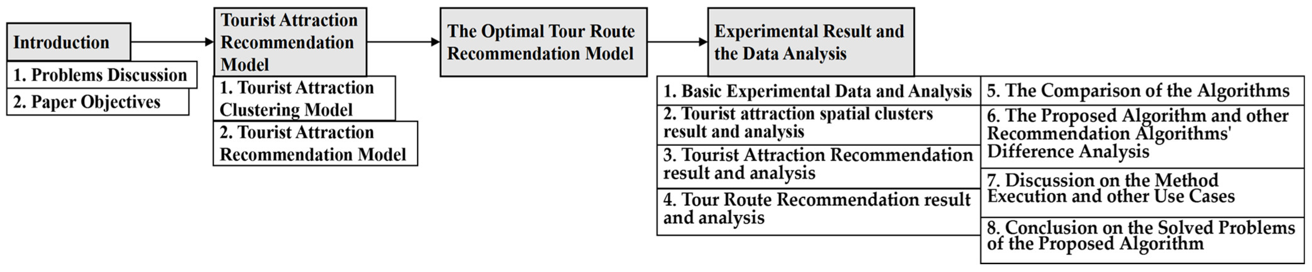
:1. Introduction
2. Tourist Attraction Recommendation Model Based on Cellular Geospatial Generating and Weighted Collaborative Filtering
2.1. The Spatial Adjacency Tourist Attraction Clustering Model Based on the Cellular Space Generating Algorithm
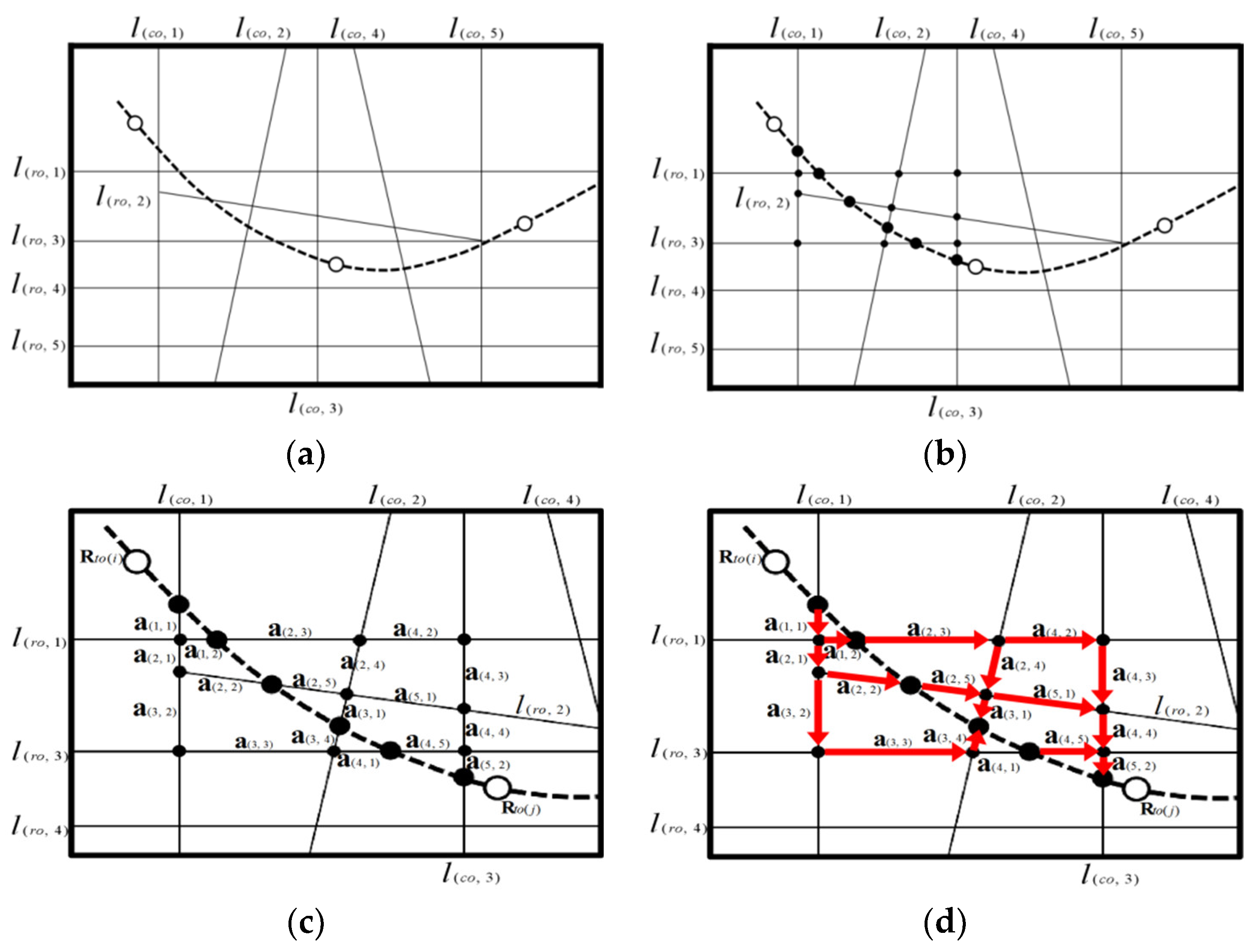
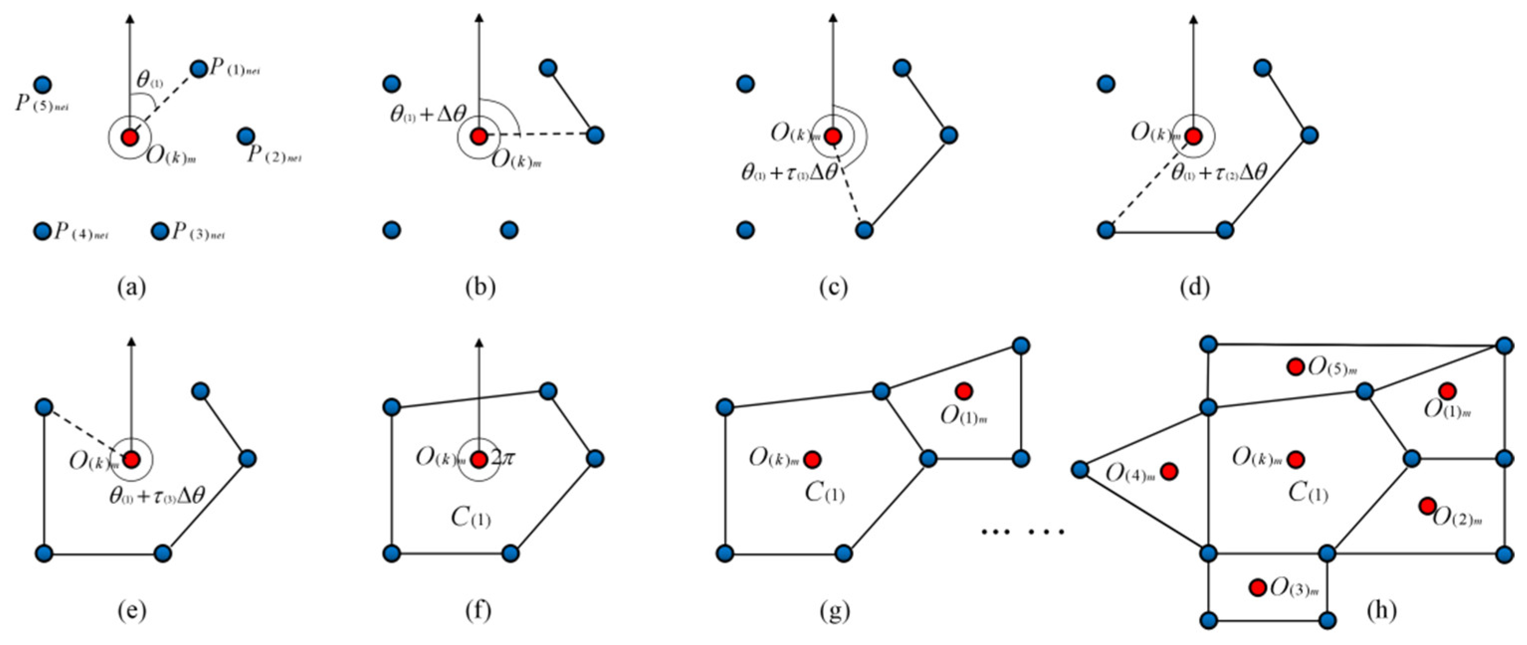
2.1.1. Tourist Attraction Cellular Space Generating Algorithm
| Algorithm 1 The cellular generating unit and cellular space generating algorithm | |
| 1: | Step 1: Generate and confirm the set for the tourist attraction cellular cores and the set for the cellular geospatial anchor points . |
| 2: | Sub-step 1: Generate the set . |
| 3: | Sub-step 2: Encode the points in set . |
| 4: | Sub-step 3: Encode the points in set . |
| 5: | Sub-step 4: Confirm the coordinate as and , as and . |
| 6: | Step 2: Generate the initial cellular generating unit . |
| 7: | Sub-step 1: Generate one ray to the north direction starting from the cellular core . |
| 8: | Sub-step 2: Set up the open list and closed list for . |
| 9: | Sub-step 3: Turn and search the neighborhood points . |
| 10: | Step 3: Generate the unit of the initial cellular generating unit . |
| 11: | Step 4: Generate all the unit of the cellular generating unit . |
| 12: | Step 5: Continue generating neighborhood units until all the points converge. |
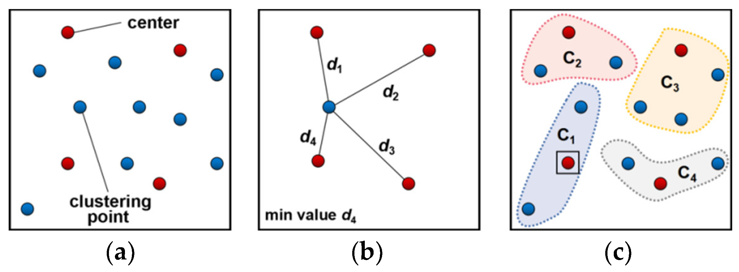
2.1.2. Tourist Attraction Clustering Algorithm Based on Geospatial Feature Attribute
| Algorithm 2 The tourist attraction clustering algorithm based on the geospatial feature attribute | |
| 1: | Step 1: Randomly and uniformly choose number of dynamic clustering centers . , noted . |
| 2: | Step 2: Store into vector , store into , note the element as and ., and . Calculate . |
| 3: | Sub-step 1: Calculate . |
| 4: | Sub-step 2: Converse , calculate . |
| 5: | Sub-step 3: Set up matrix to store in ascending order. |
| 6: | Sub-step 4: Take the minimum element of as the nearest for and absorb in . |
| 7: | Step 3: Calculate , . Take the minimum element of as the nearest for and absorb in . |
| 8: | Step 4: Converse to calculate , take the minimum element of as the nearest for and absorb in . |
2.2. Tourist Attraction Recommendation Model Based on Weighted Collaborative Filtering
- Tourist feature attribute vector : {: tour budget and cost; : traveling time; : tourist attraction hot index; : tour purpose; : transportation mode};
- Tour budget and cost : {:; : ; :; :},;
- Traveling time :{:; : ; : ;:},;
- Tourist attraction hot index :{:; : ; :;:},;
- Tour purpose :{: leisure, 0.25; : health care, 0.50; : on vacation, 0.75; : business affairs, 1.00};
- Transportation mode :{: taking taxi, 0.25; : cycling, 0.50; : walking, 0.75; : taking the public bus, 1.00}.
| Algorithm 3 Tourist attraction recommendation algorithm based on the weighted collaborative filtering | |
| 1: | Step 1: Set up tourist attraction feature attribute label word frequency matrix and word frequency storage vector . |
| 2: | Sub-step 1: Initialize the word frequency matrix . |
| 3: | Sub-step 2: Set up the evaluation data set for the historical tourists . |
| 4: | Sub-step 3: Search word frequency ~ of each row’s vector in the matrix . Define the total number of each label word frequency in the no. vector as . |
| 5: | Sub-step 4: Form matrix via . Output the vector containing each row’s vector total word frequency. |
| 6: | Step 2: Set up the tourist attraction classification interest degree set of the historical tourists. The number of historical tourists: ; the no. historical tourists: . |
| 7: | Step 3: Set up the tourist sight classification recommendation model based on the interest degree vector of the nearest neighborhood historical tourists. |
| 8: | Sub-step 1: Confirm each interest degree vector and its elements of the historical tourists related to the no. ~ location points. |
| Sub-step 2: Set up the tourist attraction classification recommendation vector . | |
| Sub-step 3: Define the recommendation degree function . The no. element of vector relates to one kind of tourist attraction classification word frequency. The average value of the no. element word frequencies calculated by the number of neighborhood historical tourists is defined as the recommendation function. . | |
| Sub-step 4: Calculate value for the number of location points . Store the values in the descending order in vector . | |
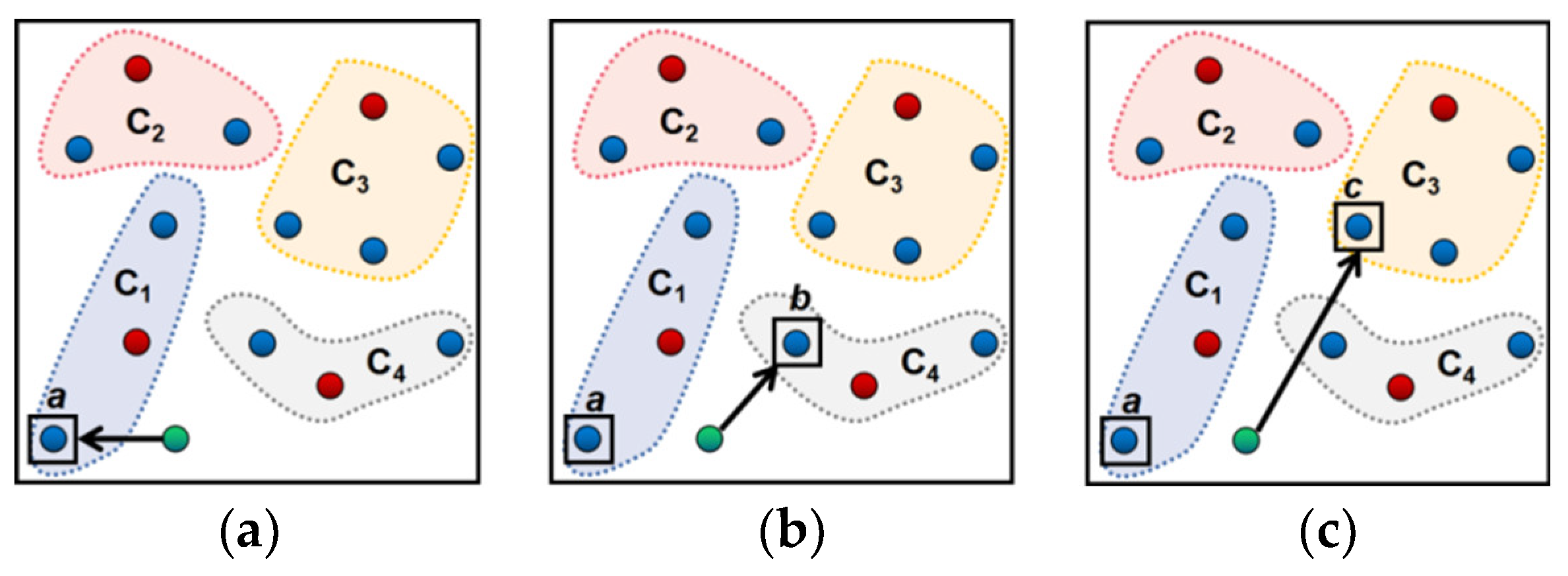
| Step 5: Set up the precise tourist attraction recommendation algorithm based on the tourist attraction search-optimized generating space. | |
| Sub-step 1: Confirm the starting point of the tour route and the tourist attraction number for the tourists. | |
| Sub-step 2: Confirm the cellular generating unit containing the starting point . | |
| Sub-step 3: Set up the Open list and the Closed list for the tourist attraction. | |
| Sub-step 4: Confirm the number of common edges of containing and its related unit and the cellular core . Search and store the feasible ones in . Delete it from the list , and store it in the list . The current tourist attraction is searched and stored in the vector . | |
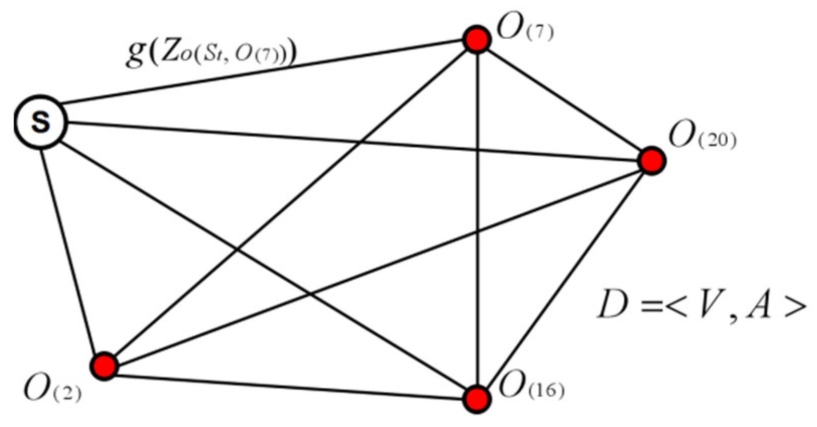
3. The Optimal Tour Route Recommendation Model Based on Precise Tourist Attraction Approach Vector Algorithm
- Step 1
- Take the closest neighborhood approach points and for the terminal points and in the set .
- Step 2
- Search the approach point set and the set .
- ①
- Search the route from the point to . Start from the point to search to the point and form the vector ; search to the point and form the vector . There is no other access route, the searching process is completed, the route is , and the approach vector set is .
- ②
- Search the route from the point to . Start from the point to search to the point and form the vector ; search to the point and form the vector ; the route is , and form the vector set . If it is judged that there is another access route, continue searching. Start from the point to search to the point and form the vector ; start from the point to search to the point and form the vector ; start from the point to search to the point and form the vector ; the route is , and form the vector set . If it is judged that there is no other access route, the searching process is completed. Judge and .
- (i)
- If , retain the access road of the and its approach vector .
- (ii)
- If , retain the access road of the and its approach vector .
- ③
- Search the route from the point to . Start from the point to search to the point and form the vector ; the route is , and form the vector set . If it is judged that there is another access road, continue searching. Start from the point to search and , pass through the points and and reach , form the vector set , and the route is . Start from the point to search ,,, pass through the points and and reach , form the vector set , and the route is . If it is judged that there is no other access route, the searching process is completed. Compare the three values , , and .
- (i)
- If the is the minimum one, retain the access road of the and its approach vector .
- (ii)
- If the is the minimum one, retain the access road of the and its approach vector .
- (iii)
- If the is the minimum one, retain the access road of the and its approach vector .
- ④
- Continue searching:
- (i)
- If searching is complete, return to step ①~③ and continue searching the route between the point and . Choose the access road of the and .
- (ii)
- If searching is not complete, continue searching the route between the point and . Choose the access road of the and . Output as the shortest access road.
- ⑤
- Confirm the set according to the route .
4. Experimental Results and Data Analysis
4.1. Basic Experimental Data Collection, Calculation and Analysis
4.1.1. The Basic Data of the Tourist Attraction Domain
4.1.2. The Basic Information Data of the Tourist Attractions and Location Points
4.1.3. Data and Result Analysis
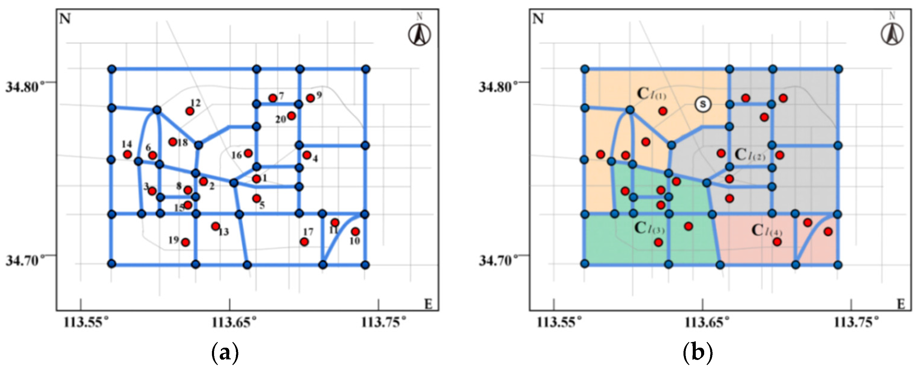
4.2. The Output Result and Analysis of the Tourist Attraction Spatial Clusters
4.2.1. The Output Result of the Tourist Attraction Cluster
4.2.2. The Data Result Analysis
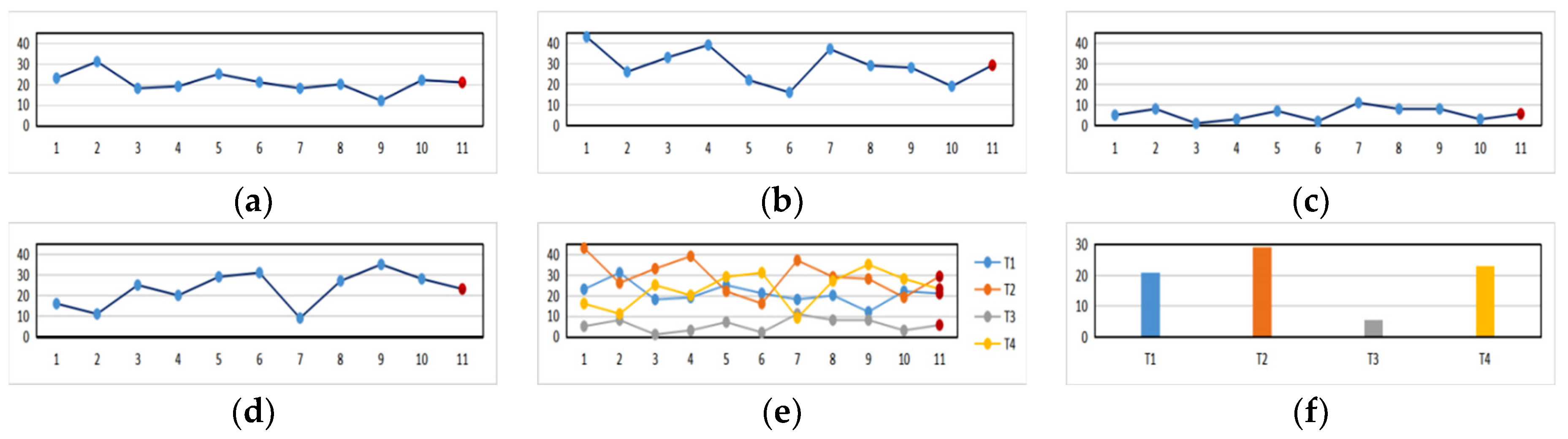
4.3. The Output Result and Analysis of the Tourist Attraction Recommendation Based on Weighted Collaborative Filtering Algorithm
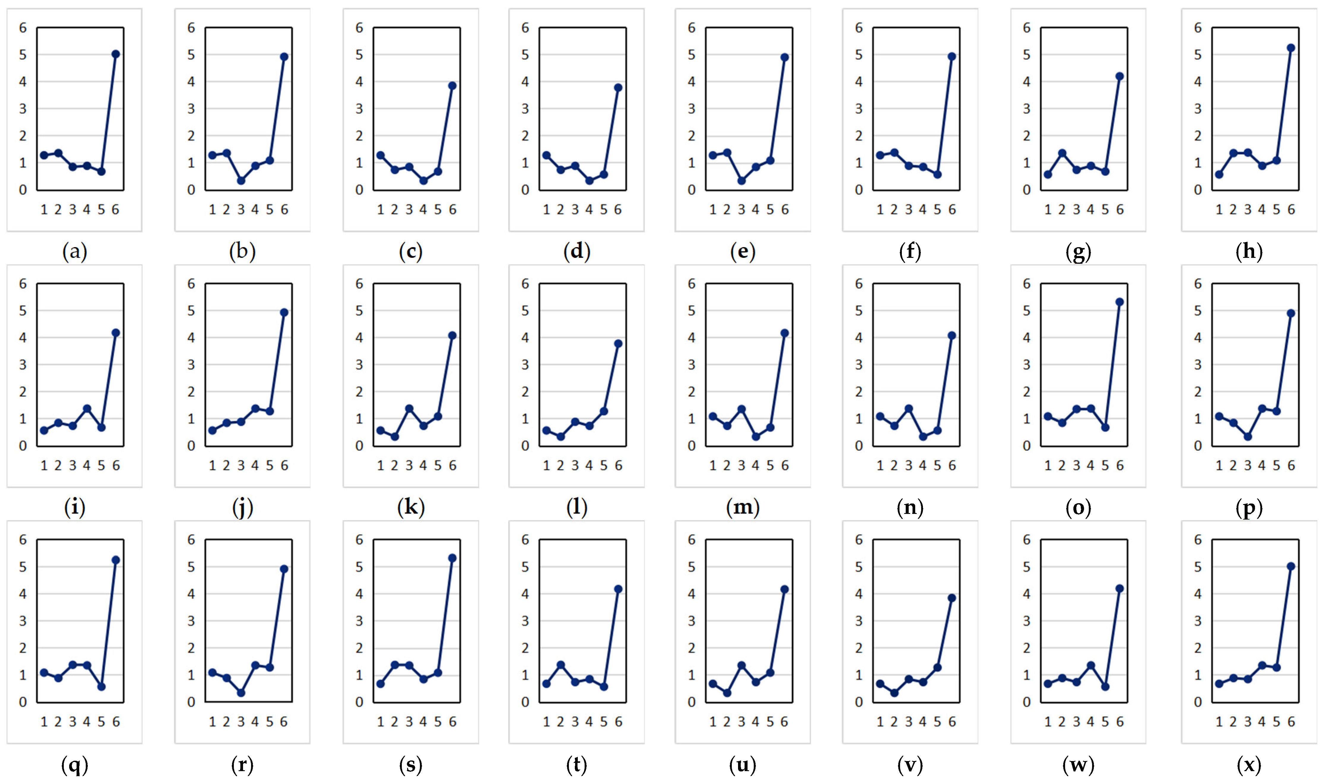
4.3.1. The Tourist Attraction Recommendation Result Based on the Weighted Collaborative Filtering Algorithm
4.3.2. The Analysis of the Data Results
4.4. The Recommendation Result and Analysis on the Optimal Tour Route Based on the Precise Tourist Attraction Approach Vector Algorithm
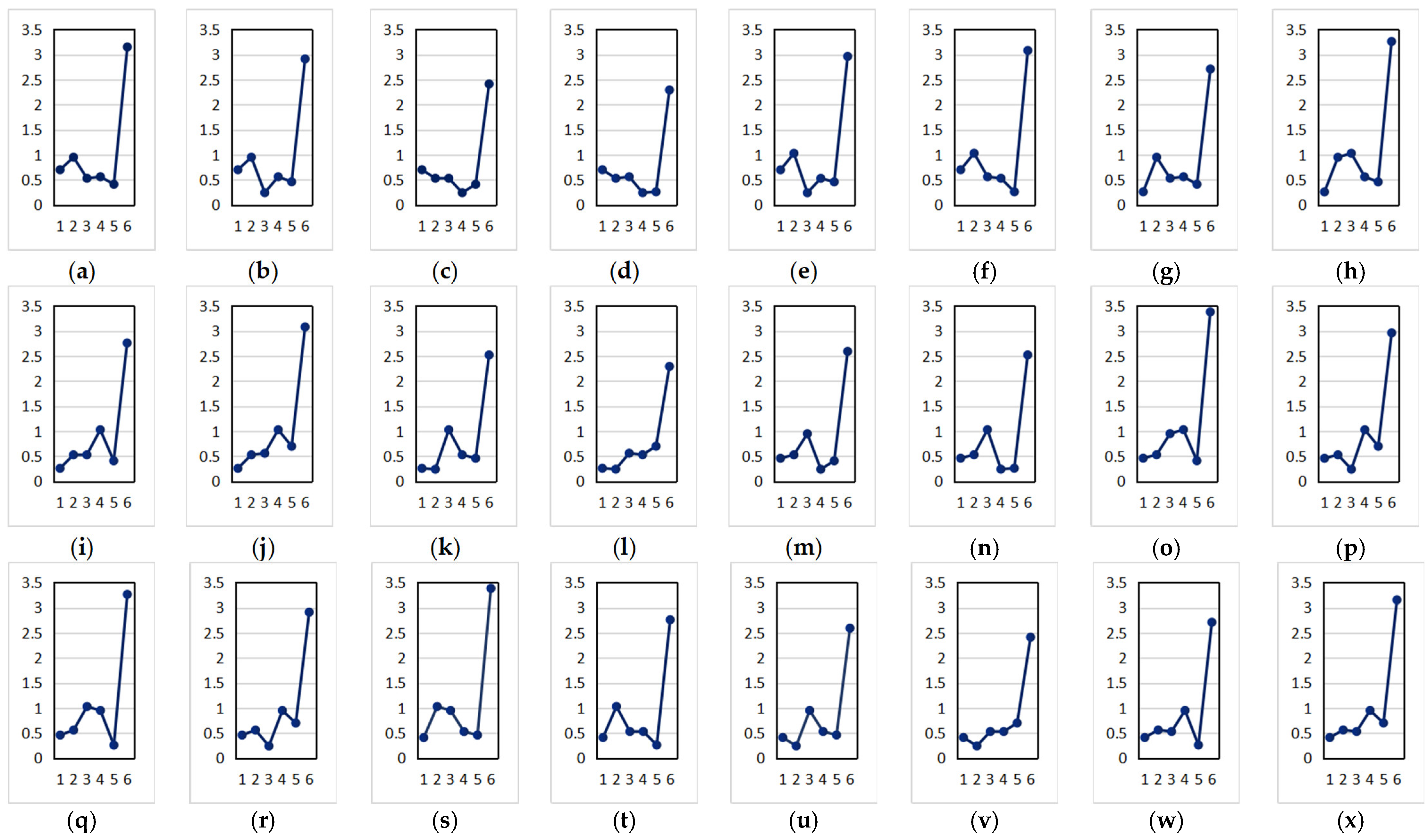
4.4.1. The Output Result of the Optimal Tour Route Recommendation Based on the Precise Tourist Attraction Approach Vector Algorithm
4.4.2. The Data Result Analysis
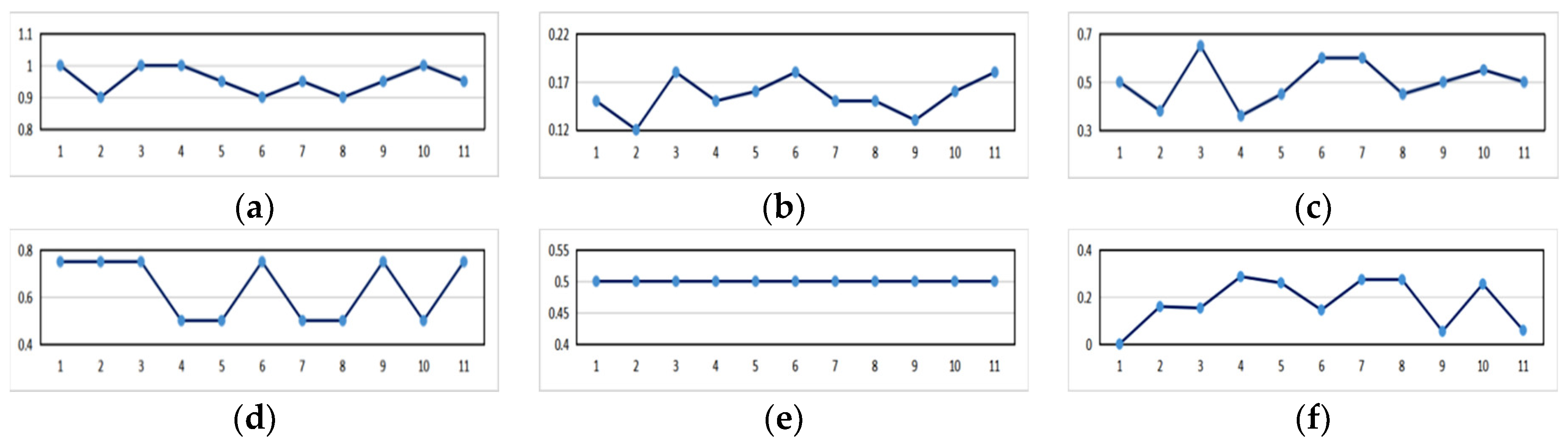
4.5. The Comparison of the Algorithms
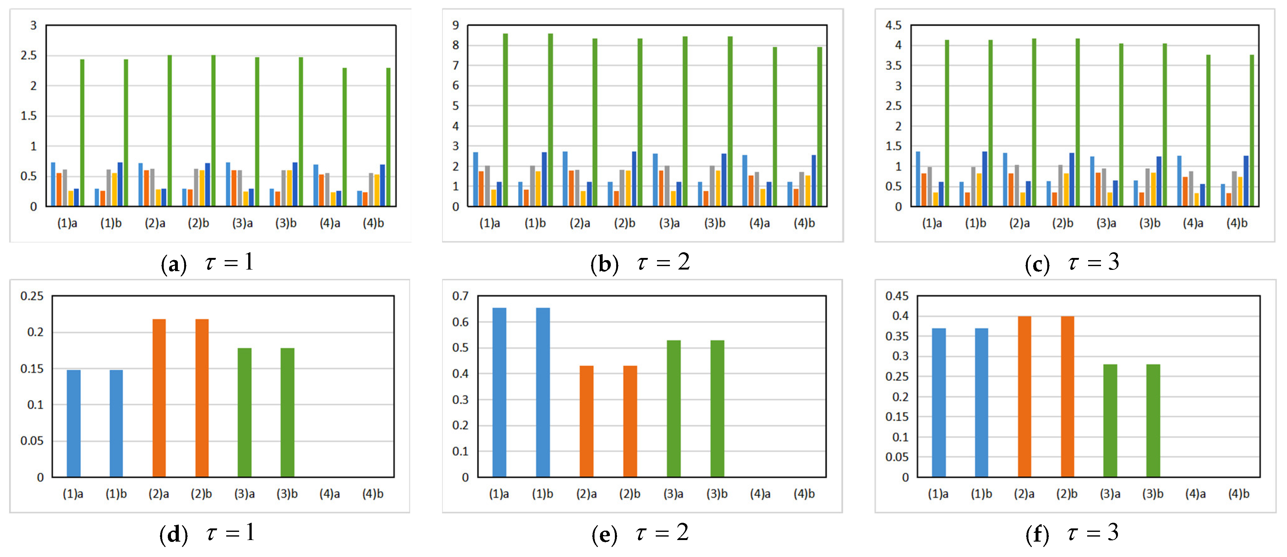
4.5.1. The Comparison Result of the Algorithm Data
4.5.2. The Data Result Analysis
4.6. The Proposed Algorithm and Other Recommendation Algorithms’ Difference Analysis
4.7. The Discussion on the Method Execution and Other Use Cases
4.8. Conclusions on the Problems Solved by the Proposed Algorithm
5. Conclusions
Author Contributions
Funding
Institutional Review Board Statement
Informed Consent Statement
Data Availability Statement
Acknowledgments
Conflicts of Interest
References
- Kato, Y.; Yamamoto, K. A Sightseeing Spot Recommendation System That Takes into Account the Visiting Frequency of Users. ISPRS Int. J. Geo Inf. 2020, 9, 411. [Google Scholar] [CrossRef]
- Ullah, F.; Shirowzhan, S.; Sepasgozar, S. Smart digital marketing capabilities for sustainable property development: A case of Malaysia. Sustainability 2020, 12, 5402. [Google Scholar]
- Lee, P.; Hunter, W.C.; Chung, N. Smart tourism city: Developments and transformations. Sustainability 2020, 12, 3958. [Google Scholar] [CrossRef]
- Mou, J.; Luo, G.; Xiong, Z. Application of Collaborative Filtering Algorithm to Tourist Attraction Recommendation. Softw. Guide 2017, 16, 186–188. [Google Scholar]
- Santos, F.; Almeida, A.; Martins, C.; Goncalves, R.; Martins, J. Using POI Functionality and Accessibility Levels for Delivering Personalized Tourism Recommendations. Comput. Environ. Urban Syst. 2019, 77, 101173. [Google Scholar] [CrossRef]
- Cui, Y.; Huang, C.; Wang, Y. Research on personalized tourist attraction recommendation based on tag and collaborative filtering. In Proceedings of the 2019 China Control and Decision Making Conference, Nanchang, China, 6 June 2019; pp. 381–385. [Google Scholar]
- Young, C.; Young, U.R.; Kyeong, K. A Recommender System based on Personal Constraints for Smart Tourism City. Asia Pac. J. Tour. Res. 2021, 26, 440–453. [Google Scholar]
- Li, G.; Zhu, T.; Yuan, T.; Hua, J.; Zhang, H. Recommendation Model of Tourist Attractions by Fusing Hierarchical Sampling and Collaborative Filtering. J. Data Acquis. Process. 2019, 34, 566–576. [Google Scholar]
- Zhou, Y.; Hu, C.; Xiong, H.; Li, L.; Wei, X. Collaborative filtering recommendation algorithm based on label of tourist spots and user preference. In Proceedings of the 2017 2nd International Conference on Machinery, Electronics and Control Simulation, Taiyuan, China, 24 June 2017; pp. 58–65. [Google Scholar]
- Nilashi, M.; Ibrahim, O.; Bagherifard, K. A Recommender System based on Collaborative Filtering Using Ontology and Dimensionality Reduction Techniques. Expert Syst. Appl. 2018, 92, 507–520. [Google Scholar] [CrossRef]
- Shi, R. Design and Implementation of Travel Recommendation System Based on Improved Collaborative Filtering Algorithm. Master’s Thesis, Hebei University of Engineering, Handan, China, 2020; p. 12. [Google Scholar]
- Chen, S.; Tian, J. Research on Tourist Attraction Recommendation model based on Collaborative Filtering Algorithm. Mod. Electron. Tech. 2020, 43, 132–135. [Google Scholar]
- Zhu, T. Research on Tourist Attractions Recommendation System Based on Deep Collaborative Filtering and Multimodal Analysis. Master’s Thesis, East China Jiaotong University, Nanchang, China, 2019; p. 5. [Google Scholar]
- Li, Y. Research on the Improvement of Collaborative Filtering Algorithm Based on Tourism Recommendation. Master’s Thesis, Qiangdao University of Science and Technology, Qingdao, China, 2019; p. 4. [Google Scholar]
- Liu, B. Research on Tourist Attractions Recommendation System Based on Hierarchical Sampling Statistics and Collaborative Filtering. Master’s Thesis, East China Jiaotong University, Nanchang, China, 2018; p. 6. [Google Scholar]
- Chen, J.; Gu, T.; Chang, L.; Bin, C.; Liang, C. A Tourist Group Recommendation Method Combining Collaborative Filtering and User Preferences. CAAI Trans. Intell. Syst. 2018, 13, 999–1005. [Google Scholar]
- Esmaeili, L.; Mardani, S.; Golpayegani, S.; Madar, Z. A novel tourism recommender system in the context of social commerce. Expert Syst. Appl. 2020, 149, 113301. [Google Scholar] [CrossRef]
- Shen, J.; Deng, C.; Gao, X. Attraction recommendation: Towards personalized tourism via collective intelligence. Neurocomputing 2016, 173, 789–798. [Google Scholar] [CrossRef]
- Sasaki, R.; Yamamoto, K. A Sightseeing Support System Using Augmented Reality and Pictograms within Urban Tourist Areas in Japan. ISPRS Int. J. Geo Inf. 2019, 8, 381. [Google Scholar] [CrossRef] [Green Version]
- Katayama, S.; Isogawa, N.; Obuchi, M.; Nishiyama, Y.; Okoshi, T.; Yonezawa, T.; Nakazawa, H.; Takashio, K.; Tokuda, H. SpoTrip: Evaluation of Information Provision System for Hidden Spots to Promote the Increase Repeat Travellers. IEICE Tech. Rep. 2017, 116, 185–192. [Google Scholar]
- Kang, S.; Lee, G.; Kim, J.; Park, D. Identifying the Spatial Structure of the Tourist Attraction System in South Korea Using GIS and Network Analysis: An Application of Anchor-Point Theory. J. Destin. Mark. Manag. 2018, 9, 358–370. [Google Scholar] [CrossRef]
- Uchida, K.; Izumi, R.; Kunieda, T.; Yamada, S.; Yonetani, K.; Gotoda, A.; Yaegashi, M. Development “KadaSola”: A Sightseeing Support System for Long Stay. In Proceedings of the 81st Annual Meeting of the Information Processing Society of Japan, Fukuoka, Japan, 14–16 March 2019; pp. 841–842. [Google Scholar]
- Mukasa, Y.; Yamamoto, K. A Sightseeing Spot Recommendation System for Urban Smart Tourism Based on Users’ Priority Conditions. J. Civ. Eng. Archit. 2019, 13, 622–640. [Google Scholar] [CrossRef] [Green Version]
- Aoike, T.; Ho, B.; Hara, T.; Ota, J.; Kurata, Y. Utilising crowd information of tourist spots in an interactive tour recommender system. In Information and Communication Technologies in Tourism; Pesonen, J., Neidhardt, J., Eds.; Springer: Berlin/Heidelberg, Germany, 2019; pp. 27–39. [Google Scholar]
- Mizutani, Y.; Yamamoto, K. A Sightseeing Spot Recommendation System That Takes into Account the Change in Circumstances of Users. ISPRS Int. J. Geo Inf. 2017, 6, 303. [Google Scholar] [CrossRef] [Green Version]
- Zhou, J.; Yamamoto, K. Development of the System to Support Tourists’ Excursion Behavior Using Augmented Reality. Int. J. Adv. Comput. Sci. Appl. 2016, 7, 197–209. [Google Scholar] [CrossRef] [Green Version]
- Noguera, J.M.; Barranco, M.J.; Segura, R.J.; Martínez, L. A Mobile 3D-GIS Hybrid Recommender System for Tourism. Inf. Sci. 2012, 215, 37–52. [Google Scholar] [CrossRef]
- Braunhofer, M.; Elahi, M.; Ricci, F. Context-Aware Places of Interest Recommendations for Mobile Users, Design, User Experience, and Usability. Theory Methods Tools Pract. Lect. Notes Comput. Sci. 2011, 6769, 531–540. [Google Scholar]
- Ying, J.J.; Lu, E.H.; Kuo, W.; Tseng, V.S. Urban Point-of-interest Recommendation by Mining User Check-in Behaviors. In Proceedings of the ACM SIGKDD International Workshop on Urban Computing, Beijing, China, 12–16 August 2012; pp. 63–70. [Google Scholar]
- Ikeda, T.; Yamamoto, K. Development of Social Recommendation GIS Tourist Spots. Int. J. Adv. Comput. Sci. Appl. 2014, 5, 8–21. [Google Scholar] [CrossRef] [Green Version]
- Nguyen, L.V.; Jung, J.J. Crowdsourcing Platform for Collecting Cognitive Feedbacks from Users: A Case Study on Movie Recommender System. In Springer Series in Reliability Engineering; Springer International Publishing: Berlin/Heidelberg, Germany, 2020; pp. 139–150. [Google Scholar]
- Nguyen, L.V.; Hong, M.S.; Jung, J.J.; Sohn, B.S. Cognitive Similarity-Based Collaborative Filtering Recommendation System. Appl. Sci. 2020, 10, 4183. [Google Scholar] [CrossRef]
- Meng, S.; Dou, W.; Zhang, X.; Chen, J. KASR: A Keyword-aware Service Recommendation Method on Map reduce for Big Data applications. IEEE Trans. Parallel Distrib. Syst. 2014, 25, 3221–3231. [Google Scholar] [CrossRef]
- Thakkar, P.; Varma, K.; Ukani, V.; Mankad, S.; Tanwar, S. Combining User-based and Item-based Collaborative Filtering using Machine Learning. Inf. Commun. Technol. Intell. Syst. 2019, 15, 173–180. [Google Scholar]
- Liu, H.; Hu, Z.; Mian, A.; Tian, H.; Zhu, X. A New User Similarity Model to Improve the Accuracy of Collaborative Filtering. Knowl.-Based Syst. 2014, 56, 156–166. [Google Scholar] [CrossRef] [Green Version]
- Bao, J.; Zheng, Y.; Wilkie, D.; Mokbel, M. Recommendations in location-based social networks: A survey. GeoInformatica 2015, 19, 525–565. [Google Scholar] [CrossRef]
- Zhang, Y.; Shi, Z.; Zuo, W.; Yue, L.; Liang, S.; Li, X.J.N. Joint Personalized Markov Chains with Social Network Embedding for Cold-Start Recommendation. Neurocomputing 2019, 386, 208–220. [Google Scholar] [CrossRef]
- Xu, M.; Liu, S. Semantic-enhanced and Context-aware Hybrid Collaborative Filtering for Event Recommendation in Event-based Social Networks. IEEE Access 2019, 7, 17493–17502. [Google Scholar] [CrossRef]
- Li, A.; She, X. The Principle, Algorithm and Application of Data Mining, 2nd ed.; Xidian University Press: Xi’an, China, 2012; p. 220. [Google Scholar]
- Zhou, X.; Xu, C.; Kimmons, B. Detecting tourism destinations using scalable geospatial analysis based on cloud computing platform. Comput. Environ. Urban Syst. 2015, 54, 144–153. [Google Scholar] [CrossRef]
- Chen, Y.-C.; Huang, H.-H.; Chiu, S.-M.; Lee, C. Joint Promotion Partner Recommendation Systems Using Data from Location-Based Social Networks. ISPRS Int. J. Geo-Inf. 2021, 10, 57. [Google Scholar] [CrossRef]
- Renjith, S.; Sreekumar, A.; Jathavedan, M. An extensive study on the evolution of context-aware personalized travel recommender systems. Inform. Process. Manag. 2020, 57, 102078. [Google Scholar] [CrossRef]
- Feng, S.; Li, X.; Zeng, Y.; Chee, Y.M. Personalized ranking metric embedding for next new poi recommendation. In Proceedings of the Twenty-Fourth International Joint Conference on Artificial Intelligence, Buenos Aires, Argentina, 25–31 July 2015; pp. 2069–2075. [Google Scholar]
- Xie, M.; Yin, H.; Wang, H.; Xu, F.; Chen, W.; Wang, S. Learning graph-based poi embedding for location-based recommendation. In Proceedings of the 25th ACM International on Conference on Information and Knowledge Management, Indianapolis, IN, USA, 24–28 October 2016; pp. 15–24. [Google Scholar]
- Zhao, S.; Zhao, T.; King, I.; Lyu, M.R. Geo-teaser: Geo-temporal sequential embedding rank for point-of-interest recom-mendation. In Proceedings of the 26th International Conference on World Wide Web Companion, Geneva, Switzerland, 3–7 April 2017; pp. 153–162. [Google Scholar]
- Memon, I.; Chen, L.; Majid, A.; Lv, M.; Hussain, I.; Chen, G. Travel recommendation using geo-tagged photos in social media for tourist. Kluw. Commun. 2015, 80, 1347–1362. [Google Scholar] [CrossRef]


| 113.673, 34.757 | 113.627, 34.745 | 113.603, 34.763 | 113.682, 34.826 | ||||
| 113.637, 34.758 | 113.663, 34.761 | 113.603, 34.742 | 113.682, 34.786 | ||||
| 113.607, 34.752 | 113.690, 34.698 | 113.603, 34.736 | 113.682, 34.763 | ||||
| 113.695, 34.767 | 113.613, 34.762 | 113.631, 34.763 | 113.682, 34.756 | ||||
| 113.671, 34.757 | 113.615, 34.715 | 113.629, 34.757 | 113.682, 34.752 | ||||
| 113.609, 34.763 | 113.681, 34.784 | 113.629, 34.742 | 113.682, 34.737 | ||||
| 113.678, 34.790 | 113.568, 34.826 | 113.629, 34.736 | 113.703, 34.737 | ||||
| 113.627, 34.746 | 113.568, 34.808 | 113.629, 34.695 | 113.703, 34.695 | ||||
| 113.685, 34.789 | 113.568, 34.794 | 113.649, 34.754 | 113.726, 34.826 | ||||
| 113.729, 34.723 | 113.568, 34.736 | 113.656, 34.737 | 113.726, 34.756 | ||||
| 113.720, 34.730 | 113.568, 34.695 | 113.665, 34.695 | 113.726, 34.737 | ||||
| 113.618, 34.781 | 113.592, 34.772 | 113.667, 34.826 | 113.726, 34.695 | ||||
| 113.643, 34.717 | 113.585, 34.736 | 113.667, 34.774 | 113.667, 34.787 | ||||
| 113.589, 34.779 | 113.594, 34.779 | 113.667, 34.756 |
| 100.00 | 1.50 | 0.50 | 0.75 | 0.50 | 0 | |
| 90.00 | 1.20 | 0.38 | 0.75 | 0.50 | 0.159 | |
| 100.00 | 1.80 | 0.65 | 0.75 | 0.50 | 0.153 | |
| 100.00 | 1.50 | 0.36 | 0.50 | 0.50 | 0.287 | |
| 95.00 | 1.60 | 0.45 | 0.50 | 0.50 | 0.260 | |
| 90.00 | 1.80 | 0.60 | 0.75 | 0.50 | 0.144 | |
| 95.00 | 1.50 | 0.60 | 0.50 | 0.50 | 0.274 | |
| 110.00 | 1.50 | 0.45 | 0.50 | 0.50 | 0.274 | |
| 95.00 | 1.30 | 0.50 | 0.75 | 0.50 | 0.054 | |
| 100.00 | 1.60 | 0.55 | 0.50 | 0.50 | 0.255 | |
| 95.00 | 1.80 | 0.50 | 0.75 | 0.50 | 0.058 |
| 23 | 43 | 5 | 16 | |
| 31 | 26 | 8 | 11 | |
| 18 | 33 | 1 | 25 | |
| 19 | 39 | 3 | 20 | |
| 25 | 22 | 7 | 29 | |
| 21 | 16 | 2 | 31 | |
| 18 | 37 | 11 | 9 | |
| 20 | 29 | 8 | 27 | |
| 12 | 28 | 8 | 35 | |
| 22 | 19 | 3 | 28 | |
| 20.9 | 29.2 | 5.6 | 23.1 |
| 0.10 | 1.00 | 0.10 | 0.10 | 1.00 | 0.10 | 0.10 | 1.00 | 0.10 | ||||
| 5.50 | 0 | 1.50 | 8.10 | 0.25 | 15.10 | 9.20 | 0.25 | 1.00 | 0.700 | 2.570 | 1.270 | |
| 1.10 | 0 | 1.50 | 2.30 | 0.34 | 6.45 | 1.20 | 0.34 | 1.00 | 0.260 | 1.215 | 0.560 | |
| 3.10 | 0 | 1.50 | 5.40 | 0.39 | 11.10 | 5.90 | 0.39 | 1.00 | 0.460 | 2.040 | 1.080 | |
| 2.10 | 0 | 2.00 | 2.30 | 0.35 | 6.45 | 2.20 | 0.35 | 1.00 | 0.410 | 1.225 | 0.670 | |
| 7.00 | 0 | 2.50 | 8.60 | 0.30 | 15.90 | 9.50 | 0.30 | 1.00 | 0.950 | 2.750 | 1.350 | |
| 3.80 | 0 | 1.50 | 4.10 | 0.23 | 9.10 | 4.00 | 0.23 | 1.00 | 0.530 | 1.550 | 0.730 | |
| 7.30 | 0 | 3.00 | 8.40 | 0.40 | 15.60 | 8.70 | 0.40 | 1.00 | 1.030 | 2.800 | 1.370 | |
| 3.30 | 0 | 2.00 | 4.20 | 0.36 | 9.30 | 3.80 | 0.36 | 1.00 | 0.530 | 1.710 | 0.840 | |
| 0.92 | 0 | 1.50 | 1.30 | 0.13 | 6.00 | 1.00 | 0.13 | 1.00 | 0.242 | 0.860 | 0.330 | |
| 3.60 | 0 | 2.00 | 4.60 | 0.37 | 9.90 | 4.10 | 0.37 | 1.00 | 0.560 | 1.820 | 0.880 | |
| 1 | 0.7, 0.95, 0.53, 0.56, 0.41 | 3.15 | 2.57, 2.75, 1.71, 1.82, 1.225 | 10.075 | 1.27, 1.35, 0.84, 0.88, 0.67 | 5.01 | |
| 2 | 0.7, 0.95, 0.242, 0.56, 0.46 | 2.912 | 2.57, 2.75, 0.86, 1.82, 2.04 | 10.040 | 1.27, 1.35, 0.33, 0.88, 1.08 | 4.91 | |
| 3 | 0.7, 0.53, 0.53, 0.242, 0.41 | 2.412 | 2.57, 1.55, 1.71, 0.86, 1.225 | 7.915 | 1.27, 0.73, 0.84, 0.33, 0.67 | 3.84 | |
| 4 | 0.7, 0.53, 0.56, 0.242, 0.26 | 2.292 | 2.57, 1.55, 1.82, 0.86, 1.215 | 8.015 | 1.27, 0.73, 0.88, 0.33, 0.56 | 3.77 | |
| 5 | 0.7, 1.03, 0.242, 0.53, 0.46 | 2.962 | 2.57, 2.8, 0.86, 1.71, 2.04 | 9.980 | 1.27, 1.37, 0.33, 0.84, 1.08 | 4.89 | |
| 6 | 0.7, 1.03, 0.56, 0.53, 0.26 | 3.080 | 2.57, 2.8, 1.82, 1.71, 1.215 | 10.115 | 1.27, 1.37, 0.88, 0.84, 0.56 | 4.92 | |
| 7 | 0.26, 0.95, 0.53, 0.56, 0.41 | 2.710 | 1.215, 2.75, 1.55, 1.82, 1.225 | 8.5600 | 0.56, 1.35, 0.73, 0.88, 0.67 | 4.19 | |
| 8 | 0.26, 0.95, 1.03, 0.56, 0.46 | 3.260 | 1.215, 2.75, 2.8, 1.82, 2.04 | 10.625 | 0.56, 1.35, 1.37, 0.88, 1.08 | 5.24 | |
| 9 | 0.26, 0.53, 0.53, 1.03, 0.41 | 2.760 | 1.215, 1.71, 1.55, 2.8, 1.225 | 8.500 | 0.56, 0.84, 0.73, 1.37, 0.67 | 4.17 | |
| 10 | 0.26, 0.53, 0.56, 1.03, 0.7 | 3.080 | 1.215, 1.71, 1.82, 2.8, 2.57 | 10.115 | 0.56, 0.84, 0.88, 1.37, 1.27 | 4.92 | |
| 11 | 0.26, 0.242, 1.03, 0.53, 0.46 | 2.522 | 1.215, 0.86, 2.8, 1.55, 2.04 | 8.465 | 0.56, 0.33, 1.37, 0.73, 1.08 | 4.07 | |
| 12 | 0.26, 0.242, 0.56, 0.53, 0.7 | 2.292 | 1.215, 0.86, 1.82, 1.55, 2.57 | 8.015 | 0.56, 0.33, 0.88, 0.73, 1.27 | 3.77 | |
| 13 | 0.46, 0.53, 0.95, 0.242, 0.41 | 2.592 | 2.04, 1.55, 2.75, 0.86, 1.225 | 8.425 | 1.08, 0.73, 1.35, 0.33, 0.67 | 4.16 | |
| 14 | 0.46, 0.53, 1.03, 0.242, 0.26 | 2.522 | 2.04, 1.55, 2.8, 0.86, 1.215 | 8.465 | 1.08, 0.73, 1.37, 0.33, 0.56 | 4.07 | |
| 15 | 0.46, 0.53, 0.95, 1.03, 0.41 | 3.380 | 2.04, 1.71, 2.75, 2.8, 1.225 | 10.525 | 1.08, 0.84, 1.35, 1.37, 0.67 | 5.31 | |
| 16 | 0.46, 0.53, 0.242, 1.03, 0.7 | 2.962 | 2.04, 1.71, 0.86, 2.8, 2.57 | 9.980 | 1.08, 0.84, 0.33, 1.37, 1.27 | 4.89 | |
| 17 | 0.46, 0.56, 1.03, 0.95, 0.26 | 3.260 | 2.04, 1.82, 2.8, 2.75, 1.215 | 10.625 | 1.08, 0.88, 1.37, 1.35, 0.56 | 5.24 | |
| 18 | 0.46, 0.56, 0.242, 0.95, 0.7 | 2.912 | 2.04, 1.82, 0.86, 2.75, 2.57 | 10.040 | 1.08, 0.88, 0.33, 1.35, 1.27 | 4.91 | |
| 19 | 0.41, 1.03, 0.95, 0.53, 0.46 | 3.380 | 1.225, 2.8, 2.75, 1.71, 2.04 | 10.525 | 0.67, 1.37, 1.35, 0.84, 1.08 | 5.31 | |
| 20 | 0.41, 1.03, 0.53, 0.53, 0.26 | 2.76 | 1.225, 2.8, 1.55, 1.71, 1.215 | 8.5 | 0.67, 1.37, 0.73, 0.84, 0.56 | 4.17 | |
| 21 | 0.41, 0.242, 0.95, 0.53, 0.46 | 2.592 | 1.225, 0.86, 2.75, 1.55, 2.04 | 8.425 | 0.67, 0.33, 1.35, 0.73, 1.08 | 4.16 | |
| 22 | 0.41, 0.242, 0.53, 0.53, 0.7 | 2.412 | 1.225, 0.86, 1.71, 1.55, 2.57 | 7.915 | 0.67, 0.33, 0.84, 0.73, 1.27 | 3.84 | |
| 23 | 0.41, 0.56, 0.53, 0.95, 0.26 | 2.71 | 1.225, 1.82, 1.55, 2.75, 1.215 | 8.56 | 0.67, 0.88, 0.73, 1.35, 0.56 | 4.19 | |
| 24 | 0.41, 0.56, 0.53, 0.95, 0.7 | 3.15 | 1.225, 1.82, 1.71, 2.75, 2.57 | 10.075 | 0.67, 0.88, 0.84, 1.35, 1.27 | 5.01 | |
| (1) BA | (2) GA | (3) SA | (4) PA | ||||||||||
|---|---|---|---|---|---|---|---|---|---|---|---|---|---|
| 1 | a | (1) a | 0.73 | 0.55 | 0.61 | 0.26 | 0.29 | 2.44 | 0.148 | ||||
| (1) b | 0.29 | 0.26 | 0.61 | 0.55 | 0.73 | 2.44 | 0.148 | ||||||
| (2) a | 0.72 | 0.6 | 0.62 | 0.28 | 0.29 | 2.51 | 0.218 | ||||||
| (2) b | 0.29 | 0.28 | 0.62 | 0.60 | 0.72 | 2.51 | 0.218 | ||||||
| b | (3) a | 0.73 | 0.60 | 0.60 | 0.25 | 0.29 | 2.47 | 0.178 | |||||
| (3) b | 0.29 | 0.25 | 0.60 | 0.60 | 0.73 | 2.47 | 0.178 | ||||||
| (4) a | 0.70 | 0.53 | 0.56 | 0.242 | 0.26 | 2.292 | -- | ||||||
| (4) b | 0.26 | 0.242 | 0.56 | 0.53 | 0.70 | 2.292 | -- | ||||||
| 2 | a | (1) a | 2.71 | 1.75 | 2.05 | 0.825 | 1.235 | 8.57 | 0.655 | ||||
| (1) b | 1.235 | 0.825 | 2.05 | 1.75 | 2.71 | 8.57 | 0.655 | ||||||
| (2) a | 2.75 | 1.785 | 1.81 | 0.765 | 1.235 | 8.345 | 0.430 | ||||||
| (2) b | 1.235 | 0.765 | 1.81 | 1.785 | 2.75 | 8.345 | 0.430 | ||||||
| b | (3) a | 2.645 | 1.775 | 2.025 | 0.775 | 1.225 | 8.445 | 0.530 | |||||
| (3) b | 1.225 | 0.775 | 2.025 | 1.775 | 2.645 | 8.445 | 0.530 | ||||||
| (4) a | 2.57 | 1.55 | 1.71 | 0.86 | 1.225 | 7.915 | -- | ||||||
| (4) b | 1.225 | 0.86 | 1.71 | 1.55 | 2.57 | 7.915 | -- | ||||||
| 3 | a | (1) a | 1.36 | 0.83 | 0.98 | 0.35 | 0.62 | 4.14 | 0.370 | ||||
| (1) b | 0.62 | 0.35 | 0.98 | 0.83 | 1.36 | 4.14 | 0.370 | ||||||
| (2) a | 1.33 | 0.82 | 1.03 | 0.35 | 0.64 | 4.17 | 0.400 | ||||||
| (2) b | 0.64 | 0.35 | 1.03 | 0.82 | 1.33 | 4.17 | 0.400 | ||||||
| b | (3) a | 1.25 | 0.85 | 0.95 | 0.35 | 0.65 | 4.05 | 0.280 | |||||
| (3) b | 0.65 | 0.35 | 0.95 | 0.85 | 1.25 | 4.05 | 0.280 | ||||||
| (4) a | 1.27 | 0.73 | 0.88 | 0.33 | 0.56 | 3.77 | -- | ||||||
| (4) b | 0.56 | 0.33 | 0.88 | 0.73 | 1.27 | 3.77 | -- | ||||||
| (1) BA | (2) GA | (3) SA | (4) PA | (min) | |||||
|---|---|---|---|---|---|---|---|---|---|
| (1) BA | (2) GA | (3) SA | (4) PA | ||||||
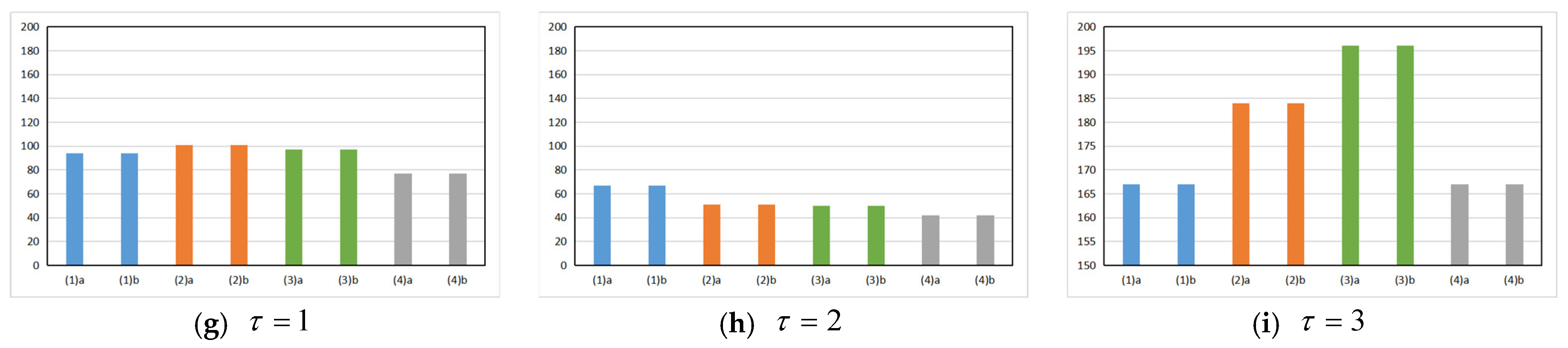
| 1 | a | 94 | 101 | 97 | 77 | ||||
| b | 94 | 101 | 97 | 77 | |||||
| 2 | a | 67 | 51 | 50 | 42 | ||||
| b | 67 | 51 | 50 | 42 | |||||
| 3 | a | 167 | 184 | 196 | 167 | ||||
| b | 167 | 184 | 196 | 167 | |||||
Publisher’s Note: MDPI stays neutral with regard to jurisdictional claims in published maps and institutional affiliations. |
© 2021 by the authors. Licensee MDPI, Basel, Switzerland. This article is an open access article distributed under the terms and conditions of the Creative Commons Attribution (CC BY) license (https://creativecommons.org/licenses/by/4.0/).
Share and Cite
Zhou, X.; Tian, J.; Peng, J.; Su, M. A Smart Tourism Recommendation Algorithm Based on Cellular Geospatial Clustering and Multivariate Weighted Collaborative Filtering. ISPRS Int. J. Geo-Inf. 2021, 10, 628. https://doi.org/10.3390/ijgi10090628
Zhou X, Tian J, Peng J, Su M. A Smart Tourism Recommendation Algorithm Based on Cellular Geospatial Clustering and Multivariate Weighted Collaborative Filtering. ISPRS International Journal of Geo-Information. 2021; 10(9):628. https://doi.org/10.3390/ijgi10090628
Chicago/Turabian StyleZhou, Xiao, Jiangpeng Tian, Jian Peng, and Mingzhan Su. 2021. "A Smart Tourism Recommendation Algorithm Based on Cellular Geospatial Clustering and Multivariate Weighted Collaborative Filtering" ISPRS International Journal of Geo-Information 10, no. 9: 628. https://doi.org/10.3390/ijgi10090628