
Improving Room-Level Location for Indoor Trajectory Tracking with Low IPS Accuracy †


1
Department of Computer Science and Engineering, Pusan National University, Pusan 46241, Korea
2
National Institute of Advanced Industrial Science and Technology (AIST), Tokyo 135-0064, Japan
*
Author to whom correspondence should be addressed.
†
This paper is an extended version of our paper published in Kim, T.; Li, K.J. Real-time Symbolic Indoor Map Matching. In Proceedings of the 9th ACM SIGSPATIAL International Workshop on Indoor Spatial Awareness, Seattle, WA, USA, 6 November 2018; ACM: New York, NY, USA, 2018, pp. 15–24.
ISPRS Int. J. Geo-Inf. 2021, 10(9), 620; https://doi.org/10.3390/ijgi10090620
Submission received: 28 July 2021
/
Revised: 3 September 2021
/
Accepted: 13 September 2021
/
Published: 16 September 2021
(This article belongs to the Special Issue Indoor Positioning and Mapping Based on 3D GIS)
Abstract
:With the development of indoor positioning methods, such as Wi-Fi positioning, geomagnetic sensor positioning, Ultra-Wideband positioning, and pedestrian dead reckoning, the area of location-based services (LBS) is expanding from outdoor to indoor spaces. LBS refers to the geographic location information of moving objects to provide the desired services. Most Wi-Fi-based indoor positioning methods provide two-dimensional (2D) or three-dimensional (3D) coordinates in 1–5 m of accuracy on average approximately. However, many applications of indoor LBS are targeted to specific spaces such as rooms, corridors, stairs, etc. Thus, they require determining a service space from a coordinate in indoor spaces. In this paper, we propose a map matching method to assign an indoor position to a unit space a subdivision of an indoor space, called USMM (Unit Space Map Matching). Map matching is a commonly used localization improvement method that utilizes spatial constraints. We consider the topological information between unit spaces and moving objects’ probabilistic properties, compared to existing room-level mappings based on sensor signals, especially received signal strength-based fingerprinting. The proposed method has the advantage of calculating the probability even if there is only one input trajectory. Last, we analyze the accuracy and performance of the proposed USMM methods by extensive experiments in real and synthetic environments. The experimental results show that our methods bring a significant improvement when the accuracy level of indoor positioning is low. In experiments, the room-level location accuracy improves by almost 30% and 23% with real and synthetic data, respectively. We conclude that USMM methods are helpful to correct valid room-level locations from given positioning locations.
1. Introduction
The development of indoor position tracking technologies and wireless communication networks has accelerated location-based services (LBS) inside buildings or subways. The LBS applications provide services and information to mobile users by utilizing their geographic location over time, such as navigation, auto check-in, and security surveillance. Like the global positioning systems (GPS) in outdoor localization, there are several indoor positioning systems (IPS) that have been proposed, such as Wi-Fi, Ultra-Wideband (UWB), Bluetooth, Radio-Frequency Identification (RFID), and inertial sensors [1,2,3]. Each of these techniques has its advantages and limitations in terms of accuracy, coverage, computational complexity, cost of deployment, and applicability. For example, UWB-based localization [4,5] can achieve centimeter-level accuracy, but it requires specific expensive hardware; Wi-Fi-based localization [6] is relatively cheap because it can use existing infrastructure. Most of these methods are reported to provide approximately 1–5 m accuracy on average, although the accuracy of these methods is unstable and affected by environmental factors, such as humidity, temperature, and other electronic devices [7,8,9]. Some state-of-the-art Wi-Fi-based localization achieved centimeter-level accuracy, but it used additional data (such as image, video, etc.) or was tested on only prepared experiment environments (such as enough line-of-sight coverage and hardware infrastructure), not real sites [3,10,11,12]. With the accuracy of IPS, the selection of an appropriate IPS corresponding to the application requirements influences the quality of services. For example, some LBS applications require centimeter-level accuracy. One example is autonomous industrial robots cooperating with each other in a manufacturing facility [13]. In such systems, robots should know each other’s position as accurately as centimeter-level. Another example is real-time interactive IoT-based smart environments, such as remotely controlling objects in a home or office using a 3D interface [14]. It needs to be a very tight match between the actual objects and their digital representation. In contrast, many LBS applications can be serviced by room-level or region-level granularity of location even though IPS accuracy is low. For example, in scenarios security control with geofencing, which detects when an object or person enters or leaves a virtual zone, specified regions can directly represent controlled zones in contrast with coordinates of moving objects (i.e., pedestrian) [15,16]. The spatial query for indoor tracking data also used a region-level location for various analyses such as hot area detection, space planning, movement pattern discovery, and so on [17,18,19]. This means room-level or region-level granularity of location is sufficient for most indoor location-aware services, unlike those in the outdoor space [17,20,21,22,23]. To represent room-level (or region-level) location information, a symbolic space model that provides qualitative human-readable descriptions as symbolic codes about moving objects based on structural entities (such as rooms, elevators, staircases) and region (or point) of interest is used [24,25,26]. Although the symbolic code can be resolved by mapping the coordinate to the nearest meaningful space, this naive approach is unattractive due to insufficient accuracy. For example, if the positioning error exceeds certain meters, we cannot tell the correct room since it could be the room next door, as shown in Figure 1. We need a map matching method for symbolic code using the moving object’s historical trajectory to get higher accuracy. According to these requirements, room-level localization has been studied. However, almost all room-level localization studies are based on sensor signals, especially Received Signal Strength (RSS)-based Wi-Fi fingerprinting [23]. Unfortunately, several IPS working on smartphones (e.g., IndoorAtlas [27], ArcGIS Indoors [28], AnyPlace [29], BuildNGO [30], and so on) provides coordinates of a pedestrian by Software Development Kit (SDK), not signal information. Therefore, we targeted developing a map matching method in the symbolic space model using coordinates information from IPS to improve room-level accuracy.
However, assuming GPS data or the like, outdoor map matching techniques in Euclidean spaces or road networks are hard to apply directly to the symbolic space model, because the road network and the indoor topology graph have different characteristics, as shown in Figure 2. Indoor spaces feature distinct entities, such as rooms, walls, doors, and staircases, and form complex indoor topology that enables and constrains movements. Therefore, we must consider the particularities of indoor topology appropriately when map matching in indoor space. Another problem is that IPS offers lower sampling frequency and only report discrete indoor locations, unlike GPS that continuously report longitude and latitude. Therefore, there is considerable uncertainty in indoor positioning data to be used to compute indoor symbolic code. This issue becomes even more challenging to deal with in the context of complex indoor topology. Thus, we must handle indoor positioning data appropriately to find indoor symbolic code effectively and efficiently. We defined a method to find symbolic code from positioning coordinates reported by IPS is called USMM (Unit Space Map Matching). We present a USMM method by the hidden Markov model to overcome the limitations of naive USMM and consequently to improve accuracy. The hidden Markov model used in this paper is configured to reflect two factors; the error range of the indoor positioning method and the connectivity between indoor spaces. The novel contributions of our work are as follows:
- We conduct an in-depth analysis of room-level localization to emphasize the importance of room-level (or region-level) map matching.
- We formulate the unit space map matching (USMM) problem as the hidden Markov model that utilized indoor map, user trajectory, and IPS’ characteristic information.
- We design and implement several USMM methods based on the hidden Markov model. Additionally, we design and implement preprocess methods to improve its accuracy.
- We evaluate USMM with a huge synthetic dataset and a real dataset collected by commercial IPS with Android-based smartphones in actual buildings to compare and analyze the proposed methods of accuracy and performance. The experiments show that the proposed methods show significant improvements in accuracy, mainly when indoor positioning accuracy is low.
The remainder of the paper is structured as follows. The related works on indoor positioning and indoor map matching are surveyed in Section 2. We define USMM and analyze the requirements of USMM in Section 3. In the next section, we introduce an intuitive USMM and discuss the limitations of this method. We proposed several methods for improving map matching accuracy by the hidden Markov model in Section 5. Section 6 and Section 7 show the experiments’ results to analyze our methods, and this paper concludes in Section 8.
2. Related Work
Location information is essential for a wide range of ubiquitous and applications for Location-Based Services (LBS). This is why the topic of determining the position of a device in indoor space has been the subject of many studies. Most of the work on indoor map matching (or indoor localization) methods has improved the accuracy of the positioning but not the symbolic map matching. This section gives an overview of some existing systems and implementations that use various IoT sensor signal values and technologies to improve positioning accuracy and achieve room-level localization. We also introduce the spatial model used in indoor localization to improve localization accuracy.
2.1. Symbolic Space Modeling
A system requires an appropriate data model representing the locations of objects situated within the environment to provide location-based services applied to indoor spaces. In this study, we used a symbolic spatial model with a place graph according to as following characteristics, strengths, and weaknesses:
- First, symbolic information provides a qualitative, human-readable description of moving objects based on structural things or points of interest (e.g., room or floor identifiers).
- Symbolic location models can reveal explicitly topological relationships between entities in the environment, such as containment, connectivity, closeness, and overlapping depending on their nature, in contrast to geometric information.
- Last, symbolic representation enables spatial and semantic reasoning at an abstract level, supporting interactions between spatial objects within indoor spaces.
Symbolic approaches have frequently attempted to model indoor environments using topological structures [31,32] (and hierarchy structures [33,34]) of indoor space, graphs derived from the connectivity and reachability between spatial units [35,36]. If we have one of the structure information, other structure information can be derived from it. For instance, a hierarchical structure of the indoor space can be derived using the containment relationship. The accuracy of symbolic location depends on the Level of Details (LoD) of the indoor data model. For instance, grid models of indoor spaces into regular grid cells with the same shape and size can represent accurate locations if it has a small cell size (e.g., 10 cm to 1 m) [37]. On the other hand, graph models that use nodes and edges for representing indoor space, especially place topology-based models, can provide location information at the structural-entity level similar to the room level [38]. It has less location accuracy compared to grid models, but each node directly indicates a space with semantic information, such as rooms, corridors, and doors. Moreover, the edges represent topology relationships between nodes. Therefore, place topology-based models are more suitable to represent symbolic information. A particular graph model can represent accurate locations, such as a graph model for pedometers [39], but it is hard to represent room-level semantic information like grid models. Moreover, a symbolic model depends on the application domain; therefore, it needs to be created and managed accordingly. Thus, managing a massive number of location symbols requires a significant modeling effort. Symbolic models are generally less accurate compare to geometric models, but context-awareness is easier to achieve as symbolic models support human-recognizable descriptions. The major shortcoming of symbolic models is the lack of geometric details on entities and places represented in space. There are several hybrid indoor spatial models proposed to overcome this shortcoming. OGC IndoorGML [40] is one of the indoor spatial models with both geometry and topology information. Therefore, the symbolic spatial model used in this study referred to the conceptual model of IndoorGML.
2.2. Room-Level Indoor Localization
The research on improving positioning accuracy is classified into three approaches: using sensor signal values (and indoor layout information), additional context information, and additional multimedia information.
- The first approach is mainly focused on filtering the sensor values. Various researches have been done so far in [41,42,43,44,45,46]. Most studies have improved positioning accuracy by filtering the values of access point (AP) signal or smartphone sensors (acceleration, gyroscope, etc.) used in the pedestrian dead reckoning (PDR) method. WILL [41] is a system that uses the PDR to determine the indoor location using APs with different Received Signal Strength (RSS) for each room. WILL considered the room’s characteristics and the relationship between rooms, but eventually, it is aimed at the coordinate level, and the positioning accuracy is ~80%. In [45], the authors proposed a Bluetooth Low Energy (BLE) beacon-based indoor navigation system for visual impairments person. The proposed system utilized the fuzzy logic framework for estimating the user’s position. The authors analyzed the performance of various versions of the fingerprinting algorithm, including fuzzy logic type 1, fuzzy KNN, fuzzy logic type 2, and traditional methods such as proximity, trilateration, the centroid for indoor localization. The fuzzy logic type 2 method outperformed all other methods; the average localization error obtained in this approach is just 0.43 m. In [46], Son et al. proposed a magnetic vector calibration algorithm that can compensate for the change of the moving direction or the grip position of a user in the three-dimensional space. As the experiment evaluation, the proposed algorithm achieves higher positioning accuracy (average positioning error is 0.66 m) and faster initial positioning because the vector fingerprint is more identifiable compared to the magnitude fingerprint.
- The second approach focuses on improving location accuracy using sensor information and map information as well as additional contextual information (landmarks, points of interest, human activity awareness, etc.). Several studies have been conducted in this regard [47,48]. APFiLoc [47] has conducted research to improve location accuracy by combining existing Wi-Fi- and PDR-based location systems with indoor landmark information (elevators, stairs, etc.). Positioning issues based on PDR with accumulated positioning errors are resolved through landmarks, and positioning accuracy is 80% when people hold their phones.
- The final approach is to improve location accuracy, using additional multimedia information (images, video, etc.). Likewise, several studies have been carried out in connection with the works in [49,50,51]. Radaelli’s research corrected the position measurement results in coordinate units, but it improved the accuracy at the room level [49]. It used a camera installed in the corridor and processed the image data to track moving objects and entrances. It corrected the location coordinates by combining the location information created using Wi-Fi wireless maps to track moving objects. However, the accuracy has not improved significantly.
In this way, previous studies are limited to indoor positioning accuracy. However, location room-level or region-level granularity is sufficient for most indoor location-aware services, unlike outdoor space. Therefore, there is currently a wealth of relevant literature [23,52,53,54,55,56,57,58] on indoor localization at room-level. However, almost all current work is based on IoT sensor signal values. Furthermore, some works need extra sensor devices. This structure cannot be easily extended in existing systems for making room-level positioning.
- A large number of indoor positioning approaches use Wi-Fi technology to take advantage of the densely installed wireless Access Points (APs) in urban areas. Biehl et al. [55] presented the LoCo framework that can provide highly accurate room-level location using a supervised classification scheme to provide high accuracy indoor room classification based on the relative ordering of pairs of APs by RSSI. A modified AdaBoost [59] algorithm was used for room-level location estimation. They trained a classifier per room in the “one-versus-all” formulation and reported 94% accuracy. However, AdaBoost is a boosting technique that cannot be parallelized for training as well as predicting. The “one-versus-all” required computation for every room. It makes Loco’s response time dependent on the building size and the number of rooms per building. Therefore, the response time of LoCo worsens directly in proportion to the number of rooms.
- Bluetooth-based positioning is also a usual approach to room-level localization. Naya et al. [52] proposed a Bluetooth-based indoor proximity detection method for nursing context-awareness. It exploits proximity between Bluetooth devices attached to people and objects for estimating room-level proximity of people and objects. The introduction of Bluetooth Low Energy (BLE) provided even more opportunities for indoor localization. Kyritsis et al. [56] presented an easy to set up BLE-based system for room localization while keeping the cost as minimal as possible. This work used RSSI of the BLE beacon and the geometry of the rooms the beacons are placed. It shows an improvement in room estimation accuracy, especially in the boundary locations of the rooms. This work’s major disadvantage is that it necessary extra devices such as BLE beacons only for positioning.
- Another way of indoor localization is by using ultrasound signals. Inspired by bats that use those signals to navigate at night, several such systems have been developed. Jaen et al. [57] performed room-level indoor positioning using different acoustic impulse responses depending on each room’s usage and structure. It can achieve very high accuracy, except for the living room. However, most of these studies require not only smartphones, but also individual devices or applications.
A large body of room-level indoor localization approaches uses RSS directly. However, almost all commercial IPS reports in the form of coordinates to a device that requests their location. Our research has focused on developing a room-level (or region-level) map matching method with the geometry of rooms, using only a sequence of coordinates of a user.
3. Preliminaries
3.1. Map Matching in Indoor Space
Map matching denotes a procedure that assigns geographical objects to locations on a digital map [60]. The most typical geographical objects are point positions obtained from a positioning system. Map matching has been studied mainly for the outdoor environment, especially road network [61,62,63]. However, the road network and the indoor graph have different properties, as shown in Figure 2. In the case of the road network, map matching aims to place the GPS positions at their “right” locations on the road segment in the map. On the other hand, in the indoor space, the goal of map matching is to place the IPS positions at their “right” locations on the unit space in the map.
The unit space map matching follows a standard pattern:
- Extract the relevant information (e.g., latitude, longitude, speed, and heading) from the record received from the IPS.
- Select the candidate unit space from the digital indoor map. Usually, the unit spaces that are within a certain error distance of the IPS position are selected.
- Use algorithm-specific heuristics to determine the most suitable unit space among the candidate unit spaces. Common weighting criteria include weight for the proximity of unit space and weight for the topology of unit spaces.
3.2. Indoor Space Locations
Indoor space is a complex space in which various spaces are combined. Indoor space has a hierarchy in which a building consists of floors and floors consisting of a set of unit spaces. A user can define unit space with various methods, such as a gird space with a fixed resolution, a Voronoi diagram, and so on. Moreover, indoor space is naturally divided into unit space like rooms, corridors, staircases, or elevators by indoor features like walls and doors. Like an outdoor space, indoor space can be expressed as a graph, such as a unit space as a node and accessibility between spaces as an edge.
Definition 1.
Indoor Space
Indoor space I is defined as a directed graph to represent an indoor accessibility graph.
is a set of nodes representing the unit spaces as below.
- Each unit space has a unique symbolic code, such as room number.
- Each unit space has a two-dimensional polygon .
- For any pairs of units , can touches but cannot intersects.
is a set of directed edges representing the connectivity between two unit spaces.
- A directed edge exists if two unit spaces () are adjacent, connected, and no other space between and , where . Note that the adjacency between two unit spaces means touches .
- has a weight , which means a pass probability from unit space to .
- always exist.
Note that “touch” and “intersect” are spatial relationship in the 9-intersects model [64].
Example 1.
Referring to the example in Figure 3b, a floor plan is divided into seven indoor unit spaces: corridor , rooms to , and staircase . According to the definition of E, a set of edge E is . Note that if a unit space is defined by room-level, accessibility is determined by the existence of a door between two unit spaces.
When we carry out map matching for a moving object in indoor space, we have to consider not only its current position collected from IPS but also its past trajectory for a better understanding of its behavior.
Definition 2.
IPS point , IPS trajectory , and IPS sub-trajectory
An IPS point is a 3-tuple , reported by an IPS about a moving object at a timestamp with a certain error and 2D point location . We assume that the pedestrian dead reckoning (PDR) is used as one of the IPS methods which have accumulation (or initialize) error according to time.
An IPS trajectory is a sequence of IPS points , where .
An IPS sub-trajectory is a contiguous subset of a IPS trajectory L, where .
3.3. Unit Space Map Matching as the Nearest One
A simple and direct approach for USMM, which we called NSMM (Nearest Space Map Matching), is to find the nearest unit space from point l collected from any indoor positioning method. As each unit space has closed geometry, as mentioned in the definition of indoor space, we can easily find the nearest space from point l. This approach depends on the accuracy of the IPS. If the indoor positioning gives low accuracy, the result of NSMM also becomes incorrect.
Note that is a shortest Euclidean distance between a point and a polygon . If the point is included in the polygon, .
Example 2.
Referring to the example in Figure 3a, a unit space is the result of NSMM as it contains point . Similarly, unit space is the result of NSMM as it is the nearest unit space from point .
On the other hand, in Figure 3b shows an IPS trajectory and its NSMM results is . However, this path is incorrect in terms of the indoor accessibility graph I; sequence is incorrect as there is no edge , described in Section 3.2.
When NSMM gives an incorrect estimation, we may correct it for better accuracy. However, there is no basis to choose one when there are several alternatives. A possible approach to resolve this problem is to select the case with a higher probability.
3.4. Vague Location
Definition 3.
Vague location
The IPS point can convert to a set of vague locations , which consists of a 3-tuple which represents a possibilityepthat is located in at a timestamp . For an arbitrary object and an arbitrary reporting time, always holds for the corresponding set .
Definition 4.
Vague location search function
Given an IPS trajectory and an indoor space , the vague location search function returns a set of vague locations .
- is an IPS trajectory,
- is an indoor accessibility graph, and
- is a set of vague locations, consists of a tuple where . represents a likelihood of be located in at timestamp .
Example 3.
Referring to the example in Figure 3b, there is an IPS trajectory , where an narrowed curve indicates a moving object’s visiting sequence (same as timestamp t) and a radius of shade circle is error e. If we assume an area of shade circle is , according to Equation (2), a set of vague locations V for is . Likewise, with next IPS point , , and , where and .
3.5. Problem Formulation
Problem 1.
Unit Space Map Matching
Given an indoor space and a previous IPS sub-trajectory where , and an IPS point , we consider possible paths Φ in the Cartesian product of all relevant vague location sets for trajectory , i.e., . For each possible path where , we can calculate its probability as as below.
The definition of USMM is . The goal of the USMM algorithm is to find the most feasible path by picking one unit space for each t.
The goal of our work is to discover proper estimation methods for the function .
Example 4.
Figure 4 shows an illustration of the USMM for the map matching problem illustrated in Figure 3b. Here, each vertical slice represents a point in time corresponding to an IPS point at timestamp . At , there is one unit space observed near as , shown as one blank dot in the first column. The blank dots are the NSMM results of each IPS point. There is a feasible moving path, from this one unit space to points on the two unit spaces near at as . We can determine connectivity between unit spaces by edge weight . Therefore, there is no connection between at and at , shown as a thick dot line. We can quickly filter those valid candidates using the indoor accessibility graph I. As the result of the Cartesian product between and , we can get a set of possible path , where . If we assume that is the same as , then we can calculate and . Therefore, . Finally, USMM results are the same as a connection of thick lines.
3.6. Requirements
When we develop USMM methods, there are several requirements to consider for online map matching as below.
- Accuracy
- When calculating the map matching accuracy for the input trajectory, USMM aims at improving the accuracy much higher than the NSMM. Even if the accuracy of the indoor positioning method is not good, the USMM method should provide a stable and high accuracy.
- Performance
- USMM should be executed within a sampling interval of IPS in mobile devices to support real-time indoor location-based services. In most cases, the sampling interval is 1 second by default.
- Data Size
- As USMM runs on mobile devices such as smartphones, the size of prepared data needed by USMM should be small enough to suitable for mobile devices.
These aspects served as the starting points of developing proper USMM methods in our work. In the following subsection, we discuss the basic ideas about how to realize these aspects.
4. Hidden Markov Model-Based Unit Space Map Matching
Map matching using HMM has been studied mainly for outdoor environments, especially road networks [61,62,63]. However, the road network and the indoor graph have different properties, as shown in Figure 2. In the road network, the goal of map matching is to match each positioning point with the proper road segment. In the previous studies, they defined the states of the HMM as individual road segments. On the other hand, HMM is usually used for map matching with fingerprinting maps of IoT sensors such as Wi-Fi in the indoor space [65,66,67]. In [66], HMM is used for position estimation based on the fusion of RSSI and movement vector observations. The goal of unit space map matching (USMM) is to match each positioning point with the proper space. There are two reasons that we apply an HMM (hidden Markov model) for USMM: First, the HMM provides a probabilistic approach. Second, the processing cost of HMM is relatively low, which is suitable for the real-time requirement of USMM, as mentioned in Section 3.6. We discuss how to apply the HMM for USMM in this section.
4.1. Hidden Markov Model for USMM
The HMM is a statistical Markov model where the system is assumed to be a Markov process with unobserved hidden states [68,69,70]. Five elements model the HMM, as follows:
- the number of (hidden) states in the model N,
- the number of distinct observation symbols per states M,
- the state transition probability distribution A,
- the observation symbol probability distribution in a state B,
- and the initial state distribution .
Given these elements, HMM can estimate the state sequence corresponding to the observation sequence. The goal of USMM is to find the most feasible sequence of unit spaces (hidden state) from a vague location (observation symbol) of the current IPS point with the past IPS trajectory. The key issues are how to configure the elements of the HMM for USMM (for the sake of simplicity, we called it HSMM).
- The
- (hidden) states: Each unit space is a hidden state of HSMM. Because hidden states denote proper unit space from a given IPS point or trajectory in USMM problem. Therefore, we denote states as , such that indicates an i-th unit space in U. Moreover, the number of states in the model is the size of U.
- The
- observation symbols per states: An observation symbol is a vague location . It means the observation symbol also represents unit space u. The individual observation symbols denote as where . Moreover, the number of observation symbols is the same as the number of states.
- The
- state transition probability distribution A: The state transition probability distribution from to is defined as below.where and are the state at timestamp and t, respectively. And the state transition probabilities have the properties as below.These probabilities are directly affected by the topographical connectivity between two unit spaces and . Therefore, we can define as a weight of edge in I.
- The
- observation symbol probability distribution B: The observation symbol probability distribution (also called emission probabilities) is a probability when a given observation symbol can be observed in a hidden state . It is defined as below.Moreover, have the properties, same as as below.has the same meaning with , which a likelihood that located on unit space at timestamp t, even if is included in . We can calculate under the assumptions as below.
- An uncertainty region for an IPS point can be represented by an indoor positioning method error e and a point position .
- For a given , we denote a geometry of uncertainty region where can be located is .
- An emission probability can be calculated by the ratio of overlapping area between a geometry of the uncertainty region and a geometry of the unit space .
From the requirements described in Section 3.6, we have to consider the previous IPS trajectory , not only the current IPS point . We resolve it simply by grouping IPS trajectory by unit spaces in which is included, then union all geometry of uncertainty region in the same group, use it as the uncertainty region of each unit space. We denote is a union of each uncertainty region of L for .Finally, we can define as below.Note that, is an area of a polygon g. is also the same as a vague location . - The
- initial state distribution :In the case of map matching, the initial state distribution gives the probability of the moving object’s first (at timestamp ) unit space over all the spaces at the beginning of the movement.This is semantically the same as the emission probability at timestamp 1. Assuming no measurements have been taken, we start at the first IPS point and have , where and .
Example 5.
Referring to the example in Figure 5, the number of hidden state N and observation symbols M is seven because the indoor space consists of seven unit spaces . For , An initial state distribution is and the others = , because there is no other space is overlapped with the observation area (a shaded area centered at in Figure 5). Assuming has equal probability, according to a degree of node in the graph I, a state transition probability can be calculated by Equation (13), e.g., . An emission probability can be calculated by Equation (11), a ratio between an area of and , e.g., .
For making more feasible and reasonable USMM results, we evaluate the probabilities of the HSMM. There are three algorithms for solving three fundamental problems using an HMM: forward algorithm, Viterbi algorithm, and forward-backward algorithm. This paper uses the forward algorithm to real-time HSMM using an IPS trajectory . However, as collected IPS points getting accumulated, an old previous trajectory becomes meaningless. For this reason, it is better to handle only a recent sub-trajectory.
This paper proposes a method to determine an affect-high period of trajectory through a sliding window. For the convenience, we denote a sub-trajectory of IPS trajectory covered by sliding window w as . As the sliding window moves through, some elements of HSMM should be updated accordingly:
- the initial state distribution should be updated using the first element of and
- the observation symbol probability distribution B should be updated according to Equation (11).
Example 6.
Figure 6 shows an example of a sliding window. Given the size of the sliding window , we only consider three most recent positions for computing the B matrix, instead of the entire trajectory. For more detail, in Figure 6a shows the case where the sliding window contains at time t. Next, in Figure 6b, when we get the most recent position at time , W have replace to . At this time, π and B should be update for getting HSMM result about .
The real-time HSMM procedure is given as Algorithm 1. As the processing time is quite short, it can easily implement in mobile devices for real-time services. We will discuss it in the next section.
| Algorithm 1 Real-Time HSMM |
Input: - I: an indoor accessibility graph as - : an IPS trajectory with last IPS point - : a last HSMM result - : a hidden Markov model for unit space map matching as a tuple - w: size of a sliding window Output: - : HSMM result (a most feasible path of ) Begin
End |
4.2. The Methods of Determining the A Matrix
The implementation of state transition probability distribution A is one of the fundamental requirements of the HSMM. With a proper definition of A, we can significantly improve the accuracy of HSMM. The first idea for the definition is based on the connectivity of the indoor accessibility graph I. Given the i-th node of the I in the Definition Section 3.2, the probability is defined as follows:
While the probability of unit space transition from to is considered as same as transition from to in Equation (13), it depends on the context of moving object normally. For example, when a moving object stays in a classroom for a while, the probability of staying in the unit space is greater than the probability of transition to another room. For this reason, we increase bigger than () of the state transition matrix when the moving object is staying in the same unit space for a while. On the contrary, we decrease when moving across different unit spaces. To reflect this property, we dynamically update the state transition matrix instead of the static transition matrix given in Equation (14) as follows:
Note that means the probability to stay in the same unit space. The parameter () is determined in a dynamic way. indicates at k-th position of a moving object collected by indoor positioning starting from , and it is recursively defined as follows:
The initial value of is given by user, for example, . It increases by every time the displacement is under , which means staying in the same unit space as explained in Figure 7
When generating matrix, a probability of transition to unconnected unit spaces is not considered. These constraints have the effect of correcting the case where it is impossible to move on the indoor layout directly. However, this is one reason that fails to generate a valid result when evaluating the probability of an IPS trajectory with considerable noise. We suggest one way with the A matrix that reduces the impact of this problem. This problem can be solved by generating a transition probability between connected unit spaces and between unconnected unit spaces. If they are unconnected to each other, the probability value should be much smaller than that of the adjacent case. is a hidden state transition probability matrix that is generated to reflect these characteristics by using an graph I and graph hop distance :
Note that means a minimum hop counts (same as minimum graph hop distance) from nodes to in U. If i and j are the same or there is no path from to , zero is returned. is a weight that sets as a denominator. Therefore, the larger the value, the smaller the value. The probability of transition to the same unit space is set to one, which is the largest value of . In other cases, if is zero, the nodes and are not linked on the indoor graph I and is zero. sets to the normalized value of where .
4.3. The Methods of Determining the B Matrix
Another of the fundamental issues of the HSMM is the determination of emission probability distribution B. As discussed in the previous Section 4.1, B can be estimated by the uncertainty regions generated from an IPS trajectory L. To use Equation (11), we should determine how to calculate , which represents an uncertainty region for an IPS point l. We propose a primary method of by a circle buffer polygon which is centered at with a size of the radius is , as shown in Figure 5. This method highly depends on the IPS error value. Unfortunately, almost all IPS does not provide its (average) error size at timestamp t. In this case, we have to set a specific value as the average IPS error value for the target space. For example, we can determine its error value with vast experiment results on the target space.
Note that is a point buffer which centered at with a fixed width . The radius of uncertainty circle region might be determined as an indoor positioning error e. However, the distribution of IPS error is unstable. Therefore, we have to consider more various condition to cover exceptional cases such as a Euclidean distance between current IPS point and previous IPS point is greater than . We assume that a Euclidean distance between an IPS point and previous IPS point is the maximum positioning error value. Then, an adaptive radius for is defined as follows:
Example 7.
Figure 8 shows an example of applying an adaptive radius. In the case of , we can see that the uncertainty region for unit space is only intersected unit spaces and when calculating with a given radius . On the other hand, as shown in a blue circle, when calculated as the adaptive radius, observation probabilities are generated for the unit spaces and , additionally. It helps to consider various paths for a given IPS trajectory.
Unlike the A matrix, the B matrix’s probability distribution depends on the input IPS trajectory. In other words, the probability distribution is not constructed for all unit spaces in an indoor layout. When evaluating this narrow probability distribution, various results are not taken into account. We have to generate a base probability distribution for the B matrix from considering all unit spaces to resolve it. For this purpose, we propose a base method of using a unit space’s geometry-based buffer :
Note that is a polygon buffer with polygon with a fixed width d. According to the concept of base method, the emission probability , defined in Equation (11), should be changed as below.
Note that is a unit space where located.
5. Indoor Distance-Based Correction
In the previous section, we introduced the basic HSMM method as one of the USMM methods. However, the indoor trajectory of moving objects can be corrected by the correction method using the spatial characteristics before doing map matching. Indoor spaces are separated by walls, and walls are often considered the most important elements of an indoor map. In this paper, we used an indoor distance constrained by the topology of spaces and the geometry of walls. There are several ways to determine indoor distance based on where the two points are located [71,72,73]. We used minimal indoor walking distance based on Doors Graph to compute the indoor distance, based on the previous works in [72]. We can easily find irregular coordinates in the given trajectory as per the requirement below.
Assumption 1.
Given two continuous coordinates from the given IPS trajectory , a minimum indoor walking distance should be smaller than a maximum indoor distance within sampling time.
When an object moves in an indoor space, the moving distance is limited by the maximum speed. According to the literature [74,75], a human’s comfortable walking speed is 1–1.5 m/s. Similarly, we can assume the maximum speed of pedestrians in indoor space as 5.0 m/s when they are running. If the moving distance of an object exceeds the maximum speed, we have to adjust the current location within the area of the maximum distance.
The problem is how to correct the irregular location which has exceeds the maximum distance. A pattern where the IPS trajectory is across rooms beside a long corridor is one of the most frequent PDR error cases in our experience. Therefore, we make an indoor distance-based correction method for revising to a more passable space such as a corridor. An algorithm for the indoor distance-based correction is as below.
Note that is length of trajectory L. We used linear interpolation to calculate Euclidean distance between two points and , . computes the nearest point of two geometries and , where on .
Algorithm 2 is consists of two phases: First, we find all candidate unit spaces according to the connectivity of unit spaces. There are two conditions to determine candidate unit space.
- topology condition: The candidate unit space should connect to (or ) which containing starting (or ending) IPS point (or ) respectively.
- degree condition: Furthermore, a degree of node in the graph I should be more than a given minimum threshold value . This condition is derived from a characteristic of the corridor which has several connections with rooms.
Second, we find the nearest point on the segment of the indoor route trajectory from the endpoint . Each segment is derived from the intersection between the candidate unit space and the indoor route trajectory . If the number of candidate unit spaces is more than two, we determine , which has the shortest distance that the Euclidean distance between and .
Example 8.
Figure 9 shows an example of correction by indoor distance. As the distance from to exceeds the maximum distance as a red solid line, we find candidate unit spaces. We can find by topology condition, but it filtered as by degree condition . Then, we find a correction point on the indoor distance route, where nearest to point . As shown in Section 6, it improves the accuracy as well.
| Algorithm 2 Indoor_Distance_Correction |
Input: - : starting and ending IPS points - : maximum indoor distance value - I: indoor accessibility graph as - : threshold value for minimum degree Output: - : modified IPS point Begin
End |
6. Experiments
We have performed an extensive experiment for USMM by the hidden Markov model. In this section, we present the results and analysis of the experiments.
6.1. Experiment Environments
In order to carry out our experiments, we prepared two sites: One is the fourth floor of Building 313 in Pusan National University campus in the Republic of Korea, which consists of 30 cells as shown in Figure 10a. The building’s layout was similar to hotels and apartments, with a long corridor and rooms of different sizes on either side of the corridor. The other is an office building with several rooms and corridors provided in VITA [76] as shown in Figure 10b. The synthetic site is similar to a real experiment site, but firewalls divide a corridor into several spaces. The test environment was given in a two-dimensional space for simplicity. We assume that they are polygon without overlapping.
The indoor positioning data was collected in two different ways:
- The real trajectories of moving objects were collected by an indoor positioning application named BuildNGO [30], which is based on a hybrid approach with various sensors (Wi-Fi, BLE, GPS, accelerometer, gyroscope, and digital compass) data with PDR. This IPS has an average positioning accuracy of 1–3 m in the official. After collecting the experiment site’s fingerprint with BuildNGO, we developed an android application to collect trajectory information using their SDK. We can get discrete coordinates of a device by setting a sampling interval as one second. Furthermore, to evaluate the positioning accuracy, users need to press a button on the android application when they walk through doors to record the corresponding timestamps. Thus, we can get the ground truth location’s symbol at each walking step by interpolating based on these doors’ locations and corresponding timestamps of encountering them.
- Indoor mobility objects generator (VITA (https://github.com/longaspire/vita (accessed on 1 November 2020))) collected the synthetic trajectories of moving objects, which generates synthetic radio signal data for APs installed in the indoor space and generates positioning data for the moving object using these wireless signal data. VITA has various options to make moving object trajectories, e.g., AP device type, deployment model, number of AP devices, number of moving objects, a maximum speed of moving object, and so on. In this experiment, we generated 180 trajectories pairs (position with a trilateration positioning algorithm [77] and ground truth) with the default setting values.
The detailed information of collected trajectories are as summarized in Table 1.
6.2. Comparison of the Accuracy
We need to determine the buffer’s size and the sliding window’s size to perform the HSMM. If we know the IPS noise size at timestamp , we can use it for buffer size. Unfortunately, we cannot get IPS noise information using Sails SDK for BuildNGO. Therefore, we used a fixed size of the buffer instead of IPS noise. We observed the relationship between the accuracy and the buffer size incrementing by 0.5 m, starting from 0.5 to end 2.5 m for real and synthetic datasets. We also observed the relationship between the accuracy and sliding window size incrementing by two, starting from 4 and ending at 40. The maximum moving distance per second for pedestrians was set to five meters, as mentioned in Section 5. Last, we distinguish the real and synthetic datasets as two groups to observe the effectiveness of and according to IPS accuracy. In this experiment, we divided groups based on the accuracy of the NSMM, i.e., NSMM accuracy is over 80 or not. The ratio of the number of correct matching positions to the total number of positions is used as the accuracy rate to evaluate the effects of each USMM method. Note that the position is represented as a symbolic code of unit space. A correct matching position is that if the USMM result of the input trajectory and the NSMM result of the ground truth trajectory are the same at a particular timestamp.
We evaluated all combination of proposed methods for HSMM:
- three A matrix setup methods:
- –
- AT: indoor graph connectivity-based,
- –
- : indoor graph minimum hop distance-based,
- –
- : staying probability-based. We set a parameter for is as below;initial probability , distance threshold m, and increment probability value .
- two B matrix setup methods:
- –
- : circle buffer used only,
- –
- : combine of cell geometry buffer and circle buffer.
Last, we also evaluated the accuracy of whether to apply an Indoor Distance-based Correction (IDC) with a minimum threshold value of the degree as five.
An important observation of the real data experiment results in Figure 11a,b. It shows that all proposed methods give significant improvements in accuracy when the position data collected indoor positioning are inaccurate (Figure 11a). In contrast, they do not show any benefit if the indoor positioning is accurate enough (Figure 11b). We can check the effect of fixed buffer size according to the IPS accuracy, especially when did not apply IDC. If IPS has low accuracy, a larger buffer size becomes more accurate. In contrast, smaller buffer size is better than a larger one if IPS has high accuracy. However, if IDC is applied, there is no significant improvement according to , but it improves accuracy compare to what did not apply. These results show that IDC trajectories are similar to natural ones, such as ground truth trajectories. As a result, there are not many corrected points compared to the original trajectory. Moreover, IDC is not effective when IPS has high accuracy because the original trajectory is already similar to the ground truth, and as we expected, the HSMM with (or ), and corrected by indoor distance shows the best accuracy for most cases in Figure 11a. The effectiveness of is not well compared to (or ), because depends on the moving object’s status. All trajectories in the real dataset are kept moving, and are not stationary. In Figure 12, we observe similar results with the Figure 11. The proposed methods give significant improvements in accuracy when the position data collected indoor positioning is inaccurate. Almost all proposed methods’ accuracy is increasing according to increment window size except . As we mentioned, the real dataset trajectory is kept moving, so it is not suitable to . The methods’ accuracy decreases when the big enough makes self-transition probability too small.
The proposed USMM methods act the same as the multi-labeled classifiers. Therefore, we calculated the Mirco-Average F1-Score [79] of each USMM method using a real dataset for performance comparison, as shown in Figure 13. In this case, we used the entire dataset, not distinguished by the accuracy of the NSMM. The results have almost the same trend as the accuracy results—applying is always better performance than not applied. The and are better than , and is better than . And the window size is not highly affected on performance, but the performance of decreased with incremental window size.
As shown in Figure 14, a simple synthetic dataset shows that almost all proposed methods get better accuracy than NSMM, similar to real dataset results as shown in Figure 11, except with method. Especially, the accuracy of HSMM with (or ) and is almost 13% higher than NSMM accuracy. One peculiar point is option’s accuracy is relatively low when IDC is applied. In our observation, the option works well when spaces are connected to one huge or long corridor. It means the performance of each option in HSMM is affected by a structure of space. Similar to real dataset results, if IDC is applied, there is no significant improvement according to . Still, it improves accuracy compare to did not apply one when using . Special cases that a moving object is staying in one space exist in the synthetic dataset. However, does not work well because it depends on a distance threshold that uses Euclidean distance between two IPS points with a certain error. The method may consider not only distance information but also other information from internal sensors of a smartphone, such as an accelerometer and gyro sensors, for the well-detecting context of the user, such as stop or move. In this paper, we only consider coordinate information, so has limitations. The highest accuracy of each method is when is 1.5 (and 2.0 with IDC). We analyzed that this result has dependent on the average error of the synthetic dataset, as mentioned in Table 1. In Figure 15, we observed similar pattern with the Figure 12. There is no big difference according to window size if the window size is big enough (over 20).
6.3. Processing Time
The processing time is also one of the important requirements of USMM methods as the objective of the USMM is to provide the located space of moving objects’ during sampling time. In particular, the processing time becomes critical, as the mobile device of the pedestrian has limited computing power. As we introduced in Section 4.2 and Section 4.3, there are two steps to do map matching; (1) setting up HSMM, (2) evaluate the given path with HSMM. First, almost all setup methods A matrix () and B matrix () can be pre-calculated and initialized. Some methods are updated A and B matrix during the set up phase, but in this case, it only updates one row in the matrix. Therefore, the time complexity of the set up phase is , N is a number of states in HSMM. Last, we used a Forward algorithm in HMM, and its time complexity is , where T is the length of the given path. However, there are few transitions (or connections) between states according to the characteristic of indoor space as shown in Figure 5 and Figure 10. T is also limited by window size w. As we mentioned in the previous section, we have implemented a proposed method (HSMM) in the Android application that collects real positioning data, where the hardware specification is as shown in Table 2. In the real experiment site, the average turnaround time was measured as 0.233 s when did not apply the method and 0.271 s with the method. These results are within the requirement given in Section 3.6.
7. Discussion
The results obtained from the real and synthetic dataset experiments show the effectiveness of the HSMM. Table 3 shows the summary of the best options in experiment results. Almost all methods of HSMM are better than NSMM when the IPS accuracy is low. In contrast, if the IPS has high accuracy, HSMM cannot get any benefit. We summarized each HSMM method and additional options in the aspect of accuracy as below.
- The effect of fixed buffer size is inversely proportional to the IPS accuracy. This means the performance of HSMM is affected by the error of IPS. If we know about IPS error size at timestamp t, the HSMM accuracy can significantly improve.
- The (or ) usually achieves good USMM accuracy.
- The does not work well because almost all trajectory data represent kept moving, and its status (moving or staying) is hard to determine only coordinate information.
- The usually working well on both synthetic and real sites. However, if a unit space is connected with a large number of unit spaces, such as a long hallway in the real site case, can achieve better than .
- The window size and USMM accuracy are proportional. However, if the is large enough, it has little effect on accuracy.
- The IDC trajectory works well on the simple site with a long hallway. The IDC algorithm is structurally working well with a huge unit space that the huge unit space is connected to multiple unit spaces, especially when it is actually in the huge unit space but is positioned in the adjacent unit space. We can expect it is useful such as hotel, school, university, hospital, etc.
However, there is a limitation in that the conducted experiment was performed on a structurally simple building. We confirmed that the topological structure of the unit space affects the accuracy of the proposed methods due to the experiment. Therefore, additional experiments in large and complex buildings such as department stores and convention centers are needed to verify the robustness of the proposed method.
8. Conclusions and Future Work
Unlike outdoor space, indoor space is surrounded by architectural components such as walls and doors. It naturally divides indoor space into a set of unit spaces such as rooms, corridors, staircases, or elevators. To properly interpret the context of moving objects and provide indoor spatial information services, we have to discover the unit space where it is located. The symbolic space model is a model for a fundamental understanding of indoor space. It means the unit space is more useful than simple coordinates.
This paper proposed several methods to discover the unit space from the position in collected from the IPS based on the hidden Markov model. An indoor distance-based correction method was also proposed to improve the accuracy of USMM. We carried out an extensive experiment to analyze the accuracy and compare the proposed methods with a real data set. The experimental results show that the proposed methods improve accuracy when the accuracy of the indoor positioning method is low. For example, when the NSMM accuracy of indoor positioning is ~57%, our HSMM method yields accuracies higher than 75%.
The contributions of our work are summarized as follows:
- Formulated the unit space map matching (USMM) problem, which translates IPS trajectory to proper unit space identifier.
- Developed several USMM methods based on the hidden Markov model, named HSMM, with three A matrix setup methods and two B matrix setup methods.
- Developed minimum indoor walking distance-based correction method as preprocess step.
- Analyze the accuracy of the HSMM methods by extensive experiments with a synthetic and real dataset. The results of experiments show that the HSMM methods show significant improvements in accuracy, mainly when the accuracy of indoor positioning (NSMM) is low.
As it is one of the first studies on USMM, several issues are to be discussed and improved to the best of our knowledge. For example, we did not consider the speed and heading of moving objects. We expect that it would be possible to considerably improve the accuracy by including these factors in our model, not only map information. We can also improve the accuracy of USMM by taking into account human activity recognition (e.g., running, climbing stairs, and so on).
We evaluated proposed methods using a simple indoor environment (consisting of a long hallway and several rooms). However, indoor environments can be more complex in the real world, such as airports and shopping malls. These complex indoor environments consist of complex shapes of space, such as polygon with holes or a large open space. The usefulness of the proposed method deteriorates in a large open space. We need to consider how to divide a complex space into meaningful unit spaces and a USMM method to overcome this issue.
Last, we considered 2D coordinates (and 2.5D coordinates) with 2D floorplans in the experiment. Nevertheless, we can extend the proposed methods to 3D space. For example, we can calculate the volume of the uncertainty region instead of the area. The experiment with 3D environments can show the utility of the proposed methods.
Author Contributions
Conceptualization, Taehoon Kim and Ki-Joune Li; methodology, Taehoon Kim, Kyoung-Sook Kim and Ki-Joune Li; software, Taehoon Kim; writing—original draft preparation, Taehoon Kim and Ki-Joune Li; writing—review and editing, Taehoon Kim, Kyoung-Sook Kim and Ki-Joune Li; visualization, Taehoon Kim; supervision, Kyoung-Sook Kim and Ki-Joune Li; project administration, Ki-Joune Li; funding acquisition, Kyoung-Sook Kim and Ki-Joune Li. All authors have read and agreed to the published version of the manuscript.
Funding
This research was supported by a grant (21NSIP-B135746-05) from National Spatial Information Research Program (NSIP) funded by Ministry of Land, Infrastructure and Transport of Korean government and partially supported by a project, JPNP18010, commissioned by the New Energy and Industrial Technology Development Organization (NEDO).
Institutional Review Board Statement
Not applicable.
Informed Consent Statement
Not applicable.
Data Availability Statement
The data presented in this study are available from the author upon reasonable request.
Conflicts of Interest
The authors declare no conflict of interest.
References
- Curran, K.; Furey, E.; Lunney, T.; Santos, J.; Woods, D.; McCaughey, A. An evaluation of indoor location determination technologies. J. Locat. Based Serv. 2011, 5, 61–78. [Google Scholar] [CrossRef]
- Xiao, J.; Zhou, Z.; Yi, Y.; Ni, L. A survey on wireless indoor localization from the device perspective. ACM Comput. Surv. (CSUR) 2016, 49, 25. [Google Scholar] [CrossRef]
- Gu, F.; Hu, X.; Ramezani, M.; Acharya, D.; Khoshelham, K.; Valaee, S.; Shang, J. Indoor localization improved by spatial context—A survey. ACM Comput. Surv. (CSUR) 2019, 52, 1–35. [Google Scholar] [CrossRef] [Green Version]
- Alavi, B.; Pahlavan, K. Modeling of the TOA-based distance measurement error using UWB indoor radio measurements. Commun. Lett. IEEE 2006, 10, 275–277. [Google Scholar] [CrossRef]
- Lymberopoulos, D.; Liu, J. The microsoft indoor localization competition: Experiences and lessons learned. IEEE Signal Process. Mag. 2017, 34, 125–140. [Google Scholar] [CrossRef]
- Bahl, P.; Padmanabhan, V.N. RADAR: An in-building RF-based user location and tracking system. In Proceedings of the INFOCOM 2000, Nineteenth Annual Joint Conference of the IEEE Computer and Communications Societies, Tel Aviv, Israel, 26–30 March 2000; Volume 2, pp. 775–784. [Google Scholar]
- Liu, H.; Darabi, H.; Banerjee, P.; Liu, J. Survey of wireless indoor positioning techniques and systems. Syst. Man Cybern. Part C Appl. Rev. IEEE Trans. 2007, 37, 1067–1080. [Google Scholar] [CrossRef]
- Stojanović, D.; Stojanović, N. Indoor localization and tracking: Methods, technologies and research challenges. Facta Univ. Ser. Autom. Control Robot. 2014, 13, 57–72. [Google Scholar]
- He, S.; Chan, S.H.G. Wi-Fi fingerprint-based indoor positioning: Recent advances and comparisons. IEEE Commun. Surv. Tutorials 2015, 18, 466–490. [Google Scholar] [CrossRef]
- Duque Domingo, J.; Cerrada, C.; Valero, E.; Cerrada, J.A. An improved indoor positioning system using RGB-D cameras and wireless networks for use in complex environments. Sensors 2017, 17, 2391. [Google Scholar] [CrossRef] [Green Version]
- Liu, F.; Liu, J.; Yin, Y.; Wang, W.; Hu, D.; Chen, P.; Niu, Q. Survey on WiFi-based indoor positioning techniques. IET Commun. 2020, 14, 1372–1383. [Google Scholar] [CrossRef]
- Koike-Akino, T.; Wang, P.; Pajovic, M.; Sun, H.; Orlik, P.V. Fingerprinting-based indoor localization with commercial MMWave WiFi: A deep learning approach. IEEE Access 2020, 8, 84879–84892. [Google Scholar] [CrossRef]
- Schroeer, G. A real-time UWB multi-channel indoor positioning system for industrial scenarios. In Proceedings of the 2018 International Conference on Indoor Positioning and Indoor Navigation (IPIN), Nantes, France, 24–27 September 2018; pp. 1–5. [Google Scholar]
- Shirehjini, A.A.N.; Semsar, A. Human interaction with IoT-based smart environments. Multimed. Tools Appl. 2017, 76, 13343–13365. [Google Scholar] [CrossRef]
- Sheth, A.; Seshan, S.; Wetherall, D. Geo-fencing: Confining Wi-Fi coverage to physical boundaries. In Proceedings of the International Conference on Pervasive Computing, Galveston, TX, USA, 9–13 March 2009; Springer: Berlin/Heidelberg, Germany, 2009; pp. 274–290. [Google Scholar]
- Rahimi, H.; Zincir-Heywood, A.N.; Gadher, B. Indoor geo-fencing and access control for wireless networks. In Proceedings of the 2013 IEEE Symposium on Computational Intelligence in Cyber Security (CICS), Singapore, 16 – 19 April 2013; pp. 1–8. [Google Scholar]
- Jensen, C.; Lu, H.; Yang, B. Indexing the trajectories of moving objects in symbolic indoor space. In Advances in Spatial and Temporal Databases; Springer: Berlin/Heidelberg, Germany, 2009; pp. 208–227. [Google Scholar]
- Lu, H.; Yang, B.; Jensen, C.S. Spatio-temporal joins on symbolic indoor tracking data. In Proceedings of the 2011 IEEE 27th International Conference on Data Engineering, Washington, DC USA, 11–16 April 2011; pp. 816–827. [Google Scholar]
- Ahmed, T.; Pedersen, T.B.; Lu, H. Finding dense locations in symbolic indoor tracking data: Modeling, indexing, and processing. GeoInformatica 2017, 21, 119–150. [Google Scholar] [CrossRef]
- Li, K. Indoor space: A new notion of space. In Web and Wireless Geographical Information Systems; Springer: Berlin/Heidelberg, Germany, 2008; pp. 1–3. [Google Scholar]
- Jiang, Y.; Pan, X.; Li, K.; Lv, Q.; Dick, R.P.; Hannigan, M.; Shang, L. Ariel: Automatic wi-fi based room fingerprinting for indoor localization. In Proceedings of the 2012 ACM Conference on Ubiquitous Computing, Pittsburgh, PA, USA, 5–8 September 2012; pp. 441–450. [Google Scholar]
- Jiang, Y.; Xiang, Y.; Pan, X.; Li, K.; Lv, Q.; Dick, R.P.; Shang, L.; Hannigan, M. Hallway based automatic indoor floorplan construction using room fingerprints. In Proceedings of the 2013 ACM International Joint Conference on Pervasive and Ubiquitous Computing, Zurich, Switzerland, 8–12 September 2013; pp. 315–324. [Google Scholar]
- Li, Y.; Williams, S.; Moran, B.; Kealy, A. Quantized rss based wi-fi indoor localization with room level accuracy. In Proceedings of the IGNSS Conference, Sydney, Australia, 7–9 February 2018; pp. 1–14. [Google Scholar]
- Li, K.; Lee, J. Indoor spatial awareness initiative and standard for indoor spatial data. In Proceedings of the IROS 2010 Workshop on Standardization for Service Robot, Taipei, Taiwan, 18 October 2010; Volume 18. [Google Scholar]
- Kang, H.; Kim, J.; Li, K. strack: Tracking in indoor symbolic space with RFID sensors. In Proceedings of the 18th SIGSPATIAL International Conference on Advances in Geographic Information Systems, San Jose, CA, USA, 2–5 November 2010; ACM: New York, NY, USA, 2010; pp. 502–505. [Google Scholar]
- Afyouni, I.; Ray, C.; Christophe, C. Spatial models for context-aware indoor navigation systems: A survey. J. Spat. Inf. Sci. 2012, 1, 85–123. [Google Scholar] [CrossRef] [Green Version]
- IndoorAtlas. Last Meter Accuracy Through Technology Fusion. Available online: https://www.indooratlas.com/positioning-technology/ (accessed on 1 February 2021).
- ArcGIS Indoors. ArcGIS Indoors. Available online: https://www.esri.com/en-us/arcgis/products/arcgis-indoors/ (accessed on 1 February 2021).
- Anyplace. Indoor Information Service, Anyplace. Available online: https://anyplace.cs.ucy.ac.cy/ (accessed on 1 February 2021).
- SAILS Technology. Indoor Navi: SAILS Technology. Available online: https://www.sailstech.com/ (accessed on 1 February 2021).
- Dürr, F.; Rothermel, K. On a location model for fine-grained geocast. In Proceedings of the International Conference on Ubiquitous Computing, Seattle, WA, USA, 12–15 October 2003; Springer: Berlin/Heidelberg, Germany, 2003; pp. 18–35. [Google Scholar]
- Hu, H.; Lee, D.L. Semantic location modeling for location navigation in mobile environment. In Proceedings of the IEEE International Conference on Mobile Data Management, 2004. Proceedings, Berkeley, CA, USA, 19–22 January 2004; pp. 52–61. [Google Scholar]
- Stoffel, E.P.; Schoder, K.; Ohlbach, H.J. Applying hierarchical graphs to pedestrian indoor navigation. In Proceedings of the 16th ACM SIGSPATIAL International Conference On Advances in Geographic Information Systems, Irvine, CA, USA, 5–7 November 2008; pp. 1–4. [Google Scholar]
- Becker, T.; Nagel, C.; Kolbe, T.H. Discussion of Euclidean Space and Cellular Space and Proposal of An Integrated Indoor Spatial Data Model; Technical Report; Institute of Geodesy and Geoinformation Science: Berlin, Germany, 2010. [Google Scholar]
- Franz, G.; Mallot, H.A.; Wiener, J.M. Graph-based models of space in architecture and cognitive science: A comparative analysis. In Proceedings of the 17th International Conference on Systems Research, Informatics and Cybernetics (INTERSYMP 2005), International Institute for Advanced Studies in Systems Research and Cybernetics, Baden-Baden, Germany, 1–7 August 2005; pp. 30–38. [Google Scholar]
- Jensen, C.; Lu, H.; Yang, B. Graph model based indoor tracking. In Proceedings of the Mobile Data Management: Systems, Services and Middleware, 2009; Tenth International Conference on IEEE, Taipei, Taiwan, 18–21 May 2009; pp. 122–131. [Google Scholar]
- Shang, J.; Hu, X.; Cheng, W.; Fan, H. GridiLoc: A backtracking grid filter for fusing the grid model with PDR using smartphone sensors. Sensors 2016, 16, 2137. [Google Scholar] [CrossRef] [Green Version]
- Li, D.; Lee, D.L. A Topology-Based Semantic Location Model for Indoor Applications. In Proceedings of the 16th ACM SIGSPATIAL International Conference on Advances in Geographic Information Systems, Irvine, CA, USA, 5–7 November 2008; Association for Computing Machinery: New York, NY, USA, 2008. [Google Scholar] [CrossRef]
- Hilsenbeck, S.; Bobkov, D.; Schroth, G.; Huitl, R.; Steinbach, E. Graph-Based Data Fusion of Pedometer and WiFi Measurements for Mobile Indoor Positioning. In Proceedings of the 2014 ACM International Joint Conference on Pervasive and Ubiquitous Computing, Seattle, DC, USA, 13–17 September 2014; Association for Computing Machinery: New York, NY, USA, 2014; pp. 147–158. [Google Scholar] [CrossRef]
- Lee, J.; Li, K.J.; Zlatanova, S.; Kolbe, T.H.; Nagel, C.; Becker, T.; Kang, H.Y. OGC® IndoorGML 1.1. Standard, Open Geospatial Consortium. 2020. Available online: https://docs.ogc.org/is/19-011r4/19-011r4.html (accessed on 1 December 2020).
- Wu, C.; Yang, Z.; Liu, Y.; Xi, W. WILL: Wireless indoor localization without site survey. Parallel Distrib. Syst. 2013, 24, 839–848. [Google Scholar]
- Xiao, Z.; Wen, H.; Markham, A.; Trigoni, N. Lightweight map matching for indoor localisation using conditional random fields. In Proceedings of the Information Processing in Sensor Networks, IPSN-14 Proceedings of the 13th International Symposium on IEEE, Berlin, Germany, 15–17 April 2014; pp. 131–142. [Google Scholar]
- Kang, W.; Han, Y. SmartPDR: Smartphone-based pedestrian dead reckoning for indoor localization. IEEE Sensors J. 2015, 15, 2906–2916. [Google Scholar] [CrossRef]
- Song, C.; Wang, J.; Yuan, G. Hidden naive bayes indoor fingerprinting localization based on best-discriminating AP selection. ISPRS Int. J. Geo-Inf. 2016, 5, 189. [Google Scholar] [CrossRef]
- Al-Madani, B.; Orujov, F.; Maskeliūnas, R.; Damaševičius, R.; Venčkauskas, A. Fuzzy logic type-2 based wireless indoor localization system for navigation of visually impaired people in buildings. Sensors 2019, 19, 2114. [Google Scholar] [CrossRef] [PubMed] [Green Version]
- Son, W.; Choi, L. Magnetic Vector Calibration for Real-Time Indoor Positioning. In Proceedings of the ICC 2020-2020 IEEE International Conference on Communications (ICC), Online, 7–11 June 2020; pp. 1–7. [Google Scholar]
- Shang, J.; Gu, F.; Hu, X.; Kealy, A. Apfiloc: An infrastructure-free indoor localization method fusing smartphone inertial sensors, landmarks and map information. Sensors 2015, 15, 27251–27272. [Google Scholar] [CrossRef] [PubMed] [Green Version]
- Guo, S.; Xiong, H.; Zheng, X. A Novel Semantic Matching Method for Indoor Trajectory Tracking. ISPRS Int. J. Geo-Inf. 2017, 6, 197. [Google Scholar] [CrossRef]
- Radaelli, L.; Moses, Y.; Jensen, C. Using cameras to improve wi-fi based indoor positioning. In Proceedings of the International Symposium on Web and Wireless Geographical Information Systems, Seoul, Korea, 29–30 May 2014; Springer: Berlin/Heidelberg, Germany, 2014; pp. 166–183. [Google Scholar]
- Xu, H.; Yang, Z.; Zhou, Z.; Shangguan, L.; Yi, K.; Liu, Y. Indoor localization via multi-modal sensing on smartphones. In Proceedings of the 2016 ACM International Joint Conference on Pervasive and Ubiquitous Computing, Heidelberg, Germany, 12–16 September 2016; ACM: New York, NY, USA, 2016; pp. 208–219. [Google Scholar]
- Uygur, I.; Miyagusuku, R.; Pathak, S.; Moro, A.; Yamashita, A.; Asama, H. Robust and efficient indoor localization using sparse semantic information from a spherical camera. Sensors 2020, 20, 4128. [Google Scholar] [CrossRef] [PubMed]
- Naya, F.; Noma, H.; Ohmura, R.; Kogure, K. Bluetooth-based indoor proximity sensing for nursing context awareness. In Proceedings of the Ninth IEEE International Symposium on Wearable Computers (ISWC’05), Osaka, Japan, 18–21 October 2005; pp. 212–213. [Google Scholar]
- Chon, J.; Cha, H. Lifemap: A smartphone-based context provider for location-based services. IEEE Pervasive Comput. 2011, 10, 58–67. [Google Scholar] [CrossRef]
- Chen, Y.; Lymberopoulos, D.; Liu, J.; Priyantha, B. FM-based indoor localization. In Proceedings of the 10th International Conference on Mobile Systems, Applications, and Services, Low Wood Bay, Lake District, UK, 26–28 June 2012; pp. 169–182. [Google Scholar]
- Biehl, J.T.; Cooper, M.; Filby, G.; Kratz, S. Loco: A ready-to-deploy framework for efficient room localization using wi-fi. In Proceedings of the 2014 ACM International Joint Conference on Pervasive and Ubiquitous Computing, Seattle, WA, USA, 13–17 September 2014; pp. 183–187. [Google Scholar]
- Kyritsis, A.I.; Kostopoulos, P.; Deriaz, M.; Konstantas, D. A BLE-based probabilistic room-level localization method. In Proceedings of the 2016 International Conference on Localization and GNSS (ICL-GNSS), Barcelona, Spain, 28–30 June 2016; pp. 1–6. [Google Scholar]
- Jaén, L.; Álvarez, F.; Aguilera, T.; García, J. Room-level indoor positioning based on acoustic impulse response identification. In Proceedings of the Indoor Positioning and Indoor Navigation (IPIN), 2017 International Conference on IEEE, Sapporo, Japan, 18–21 September 2017; pp. 1–4. [Google Scholar]
- Akram, B.A.; Akbar, A.H.; Shafiq, O. HybLoc: Hybrid indoor Wi-Fi localization using soft clustering-based random decision forest ensembles. IEEE Access 2018, 6, 38251–38272. [Google Scholar] [CrossRef]
- Hastie, T.; Rosset, S.; Zhu, J.; Zou, H. Multi-class adaboost. Stat. Its Interface 2009, 2, 349–360. [Google Scholar] [CrossRef] [Green Version]
- Jensen, C.S.; Tradišauskas, N. Map Matching. In Encyclopedia of Database Systems; Springer: Boston, MA, USA, 2009; pp. 1692–1696. [Google Scholar] [CrossRef]
- Newson, P.; Krumm, J. Hidden Markov map matching through noise and sparseness. In Proceedings of the 17th ACM SIGSPATIAL International Conference on Advances in Geographic Information Systems, Seattle, WA, USA, 4–6 November 2009; ACM: New York, NY, USA, 2009; pp. 336–343. [Google Scholar]
- Goh, C.; Dauwels, J.; Mitrovic, N.; Asif, M.; Oran, A.; Jaillet, P. Online map-matching based on hidden markov model for real-time traffic sensing applications. In Proceedings of the Intelligent Transportation Systems (ITSC), 2012 15th International IEEE Conference on IEEE, Anchorage, AK, USA, 16–19 September 2012; pp. 776–781. [Google Scholar]
- Luo, A.; Chen, S.; Xv, B. Enhanced map-matching algorithm with a hidden Markov model for mobile phone positioning. ISPRS Int. J. Geo-Inf. 2017, 6, 327. [Google Scholar] [CrossRef] [Green Version]
- Egenhofer, M.J.; Franzosa, R.D. Point-set topological spatial relations. Int. J. Geogr. Inf. Syst. 1991, 5, 161–174. [Google Scholar] [CrossRef] [Green Version]
- Seitz, J.; Jahn, J.; Boronat, J.G.; Vaupel, T.; Meyer, S.; Thielecke, J. A hidden markov model for urban navigation based on fingerprinting and pedestrian dead reckoning. In Proceedings of the 2010 13th International Conference on Information Fusion, Edinburgh, UK, 26–29 July 2010; pp. 1–8. [Google Scholar]
- Hoang, M.K.; Schmalenstroeer, J.; Drueke, C.; Vu, D.T.; Haeb-Umbach, R. A hidden Markov model for indoor user tracking based on WiFi fingerprinting and step detection. In Proceedings of the 21st European Signal Processing Conference (EUSIPCO 2013), Marrakech, Morocco, 9–13 September 2013; pp. 1–5. [Google Scholar]
- Tiku, S.; Pasricha, S.; Notaros, B.; Han, Q. A Hidden Markov Model based smartphone heterogeneity resilient portable indoor localization framework. J. Syst. Archit. 2020, 108, 101806. [Google Scholar] [CrossRef]
- Baum, L.; Petrie, T. Statistical inference for probabilistic functions of finite state Markov chains. Ann. Math. Stat. 1966, 37, 1554–1563. [Google Scholar] [CrossRef]
- Rabiner, L.; Juang, B. An introduction to hidden Markov models. IEEE ASSP Mag. 1986, 3, 4–16. [Google Scholar] [CrossRef]
- Rabiner, L. A tutorial on hidden Markov models and selected applications in speech recognition. Proc. IEEE 1989, 77, 257–286. [Google Scholar] [CrossRef]
- Yuan, W.; Schneider, M. Supporting Continuous Range Queries in Indoor Space. In Proceedings of the 2010 Eleventh International Conference on Mobile Data Management, Kansas City, MO, USA, 23–26 May 2010; pp. 209–214. [Google Scholar]
- Yang, B.; Lu, H.; Jensen, C.S. Probabilistic threshold k nearest neighbor queries over moving objects in symbolic indoor space. In Proceedings of the 13th International Conference on Extending Database Technology, Lausanne, Switzerland, 22–26 March 2010; pp. 335–346. [Google Scholar]
- Kang, H.; Li, K. A Standard Indoor Spatial Data Model—OGC IndoorGML and Implementation Approaches. ISPRS Int. J. Geo-Inf. 2017, 6, 116. [Google Scholar] [CrossRef]
- Bohannon, R.W. Comfortable and maximum walking speed of adults aged 20–79 years: Reference values and determinants. Age Ageing 1997, 26, 15–19. [Google Scholar] [CrossRef] [PubMed] [Green Version]
- Fritz, S.; Lusardi, M. White paper: “Walking speed: The sixth vital sign”. J. Geriatr. Phys. Ther. 2009, 32, 2–5. [Google Scholar] [CrossRef] [Green Version]
- Li, H.; Lu, H.; Chen, X.; Chen, G.; Chen, K.; Shou, L. Vita: A versatile toolkit for generating indoor mobility data for real-world buildings. Proc. VLDB Endow. 2016, 9, 1453–1456. [Google Scholar] [CrossRef] [Green Version]
- Bose, A.; Foh, C.H. A practical path loss model for indoor WiFi positioning enhancement. In Proceedings of the 2007 6th International Conference on Information, Communications & Signal Processing, Singapore, 10–13 December 2007; pp. 1–5. [Google Scholar]
- ISO. Industry Foundation Classes (IFC) for Data Sharing in the Construction and Facility Management Industries—Part 1: Data Schema. In The Standard; International Organization for Standardization: Geneva, Switzerland, 2018. [Google Scholar]
- Grandini, M.; Bagli, E.; Visani, G. Metrics for multi-class classification: An overview. arXiv 2020, arXiv:2008.05756. [Google Scholar]
Figure 1.
Example of indoor positioning trajectory. A solid line represents the trajectory, and an arrow indicates the visiting sequence. A dotted line denotes an actual traveled path.
Figure 1.
Example of indoor positioning trajectory. A solid line represents the trajectory, and an arrow indicates the visiting sequence. A dotted line denotes an actual traveled path.
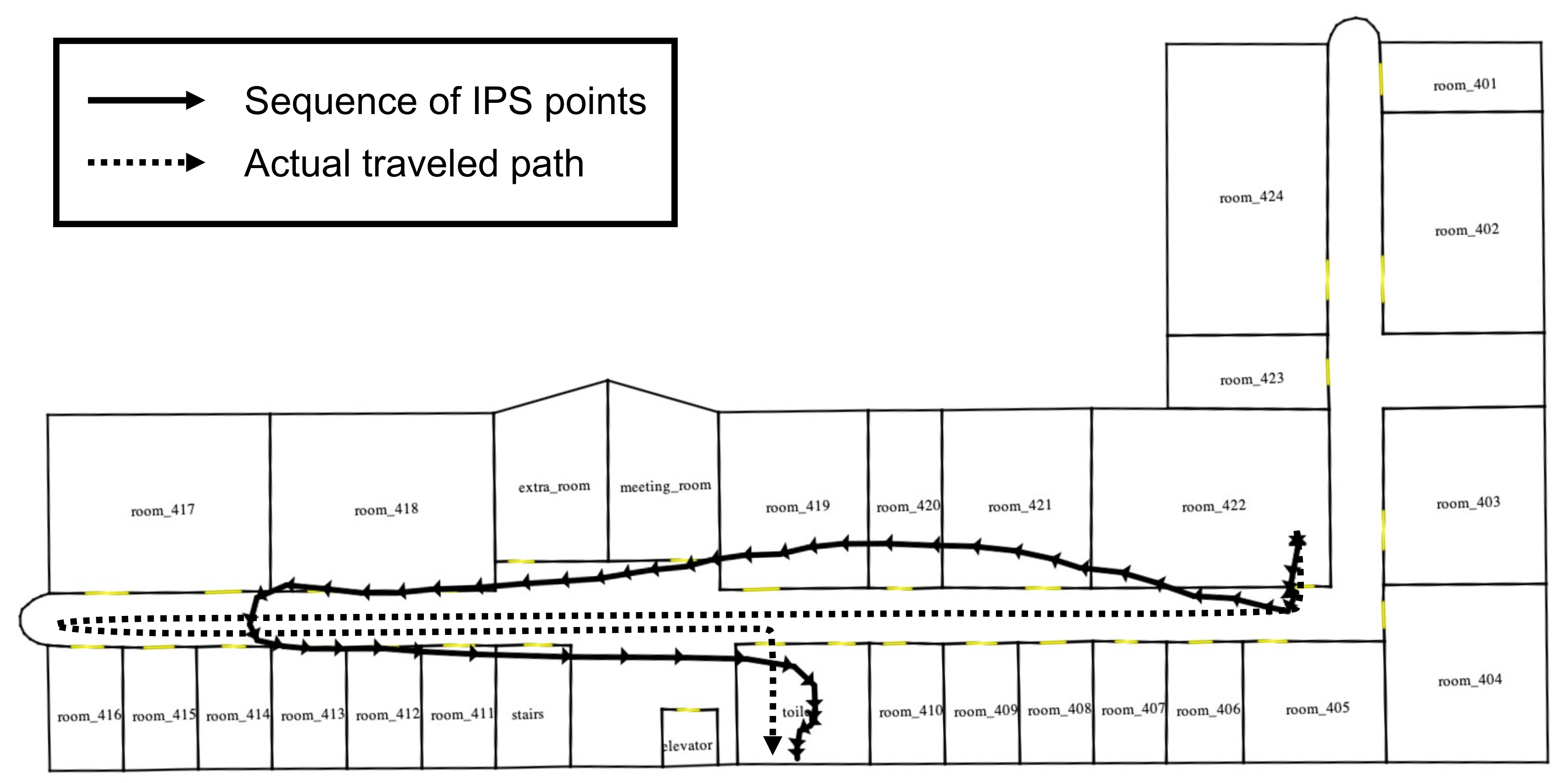
Figure 2.
Comparison of outdoor and indoor map matching methods.

Figure 3.
Example of indoor space and positioning locations.
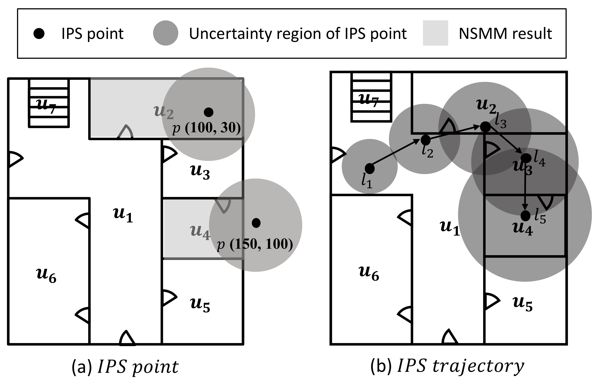
Figure 4.
Example of USMM process.

Figure 5.
Example of emission (and initial state) probability estimation.

Figure 6.
Example of applying a sliding window.

Figure 7.
Example of moving state determination of moving objects.
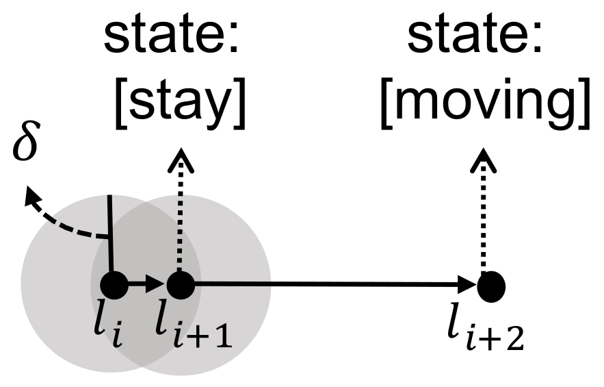
Figure 8.
Example of adaptive radius of buffer.

Figure 9.
Example of indoor distance-based correction.

Figure 10.
Layout of experiment sites.

Figure 11.
Average accuracy of USMM depending on fixed buffer size (real data).

Figure 12.
Average accuracy of USMM depending on window size (real data).

Figure 13.
Performance comparison between USMM methods (using real data)
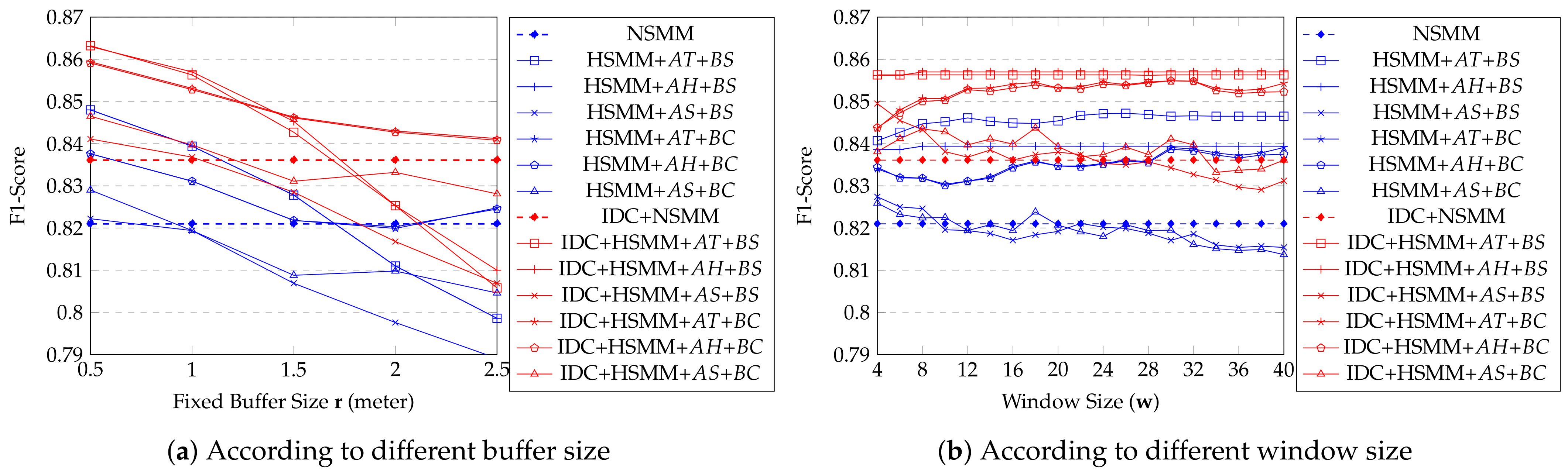
Figure 14.
Average accuracy of USMM depending on fixed buffer size (simple synthetic data).

Figure 15.
Average accuracy of USMM depending on window size (simple synthetic data).


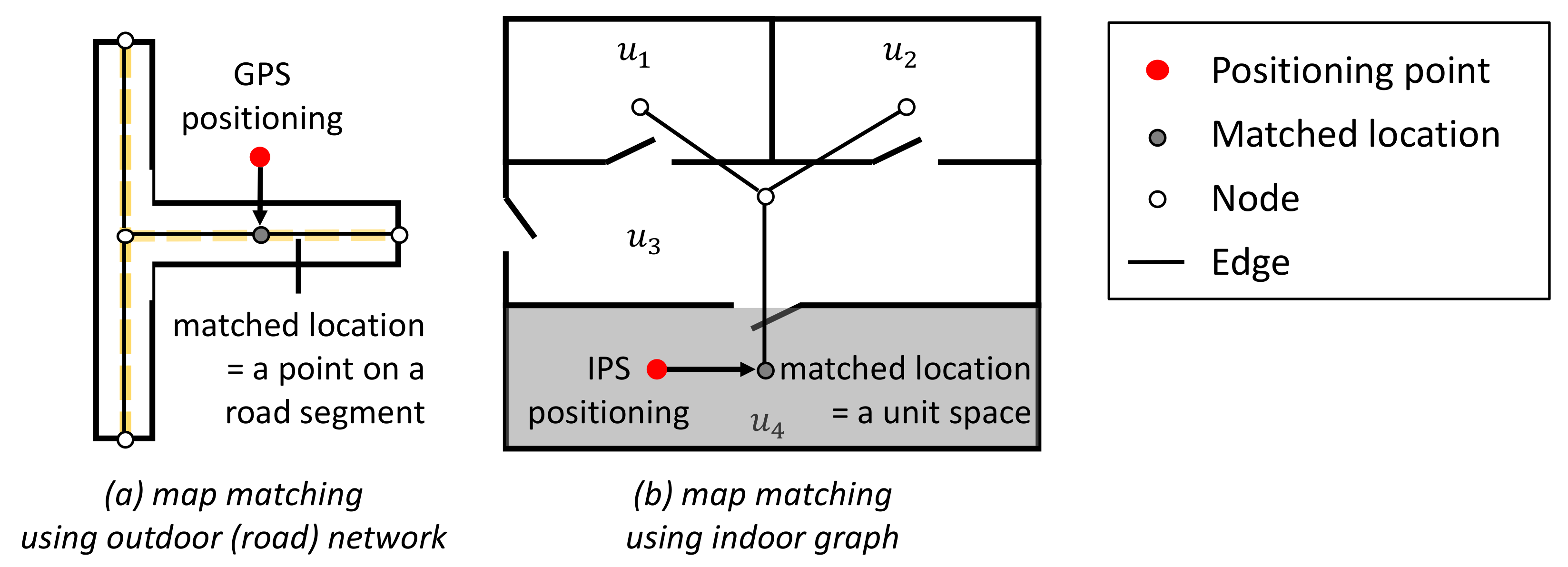
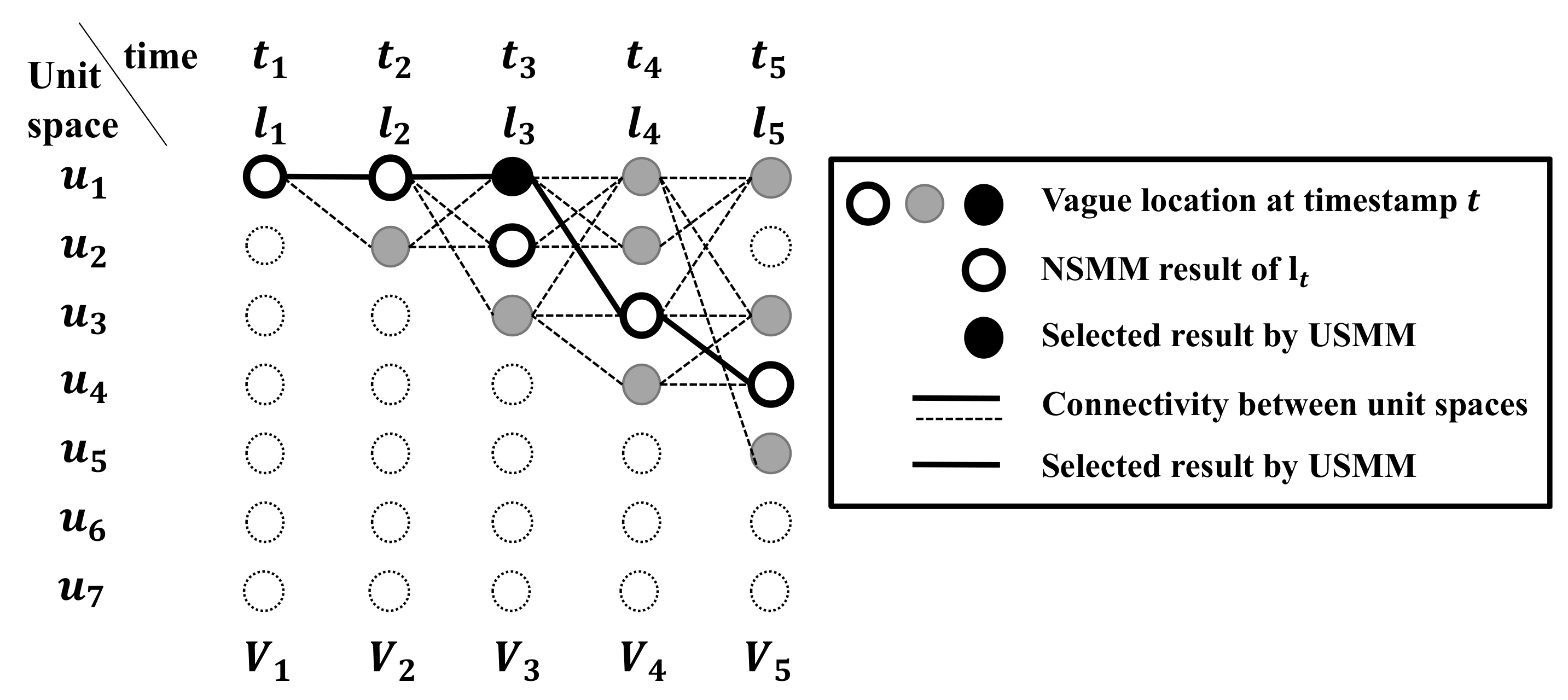
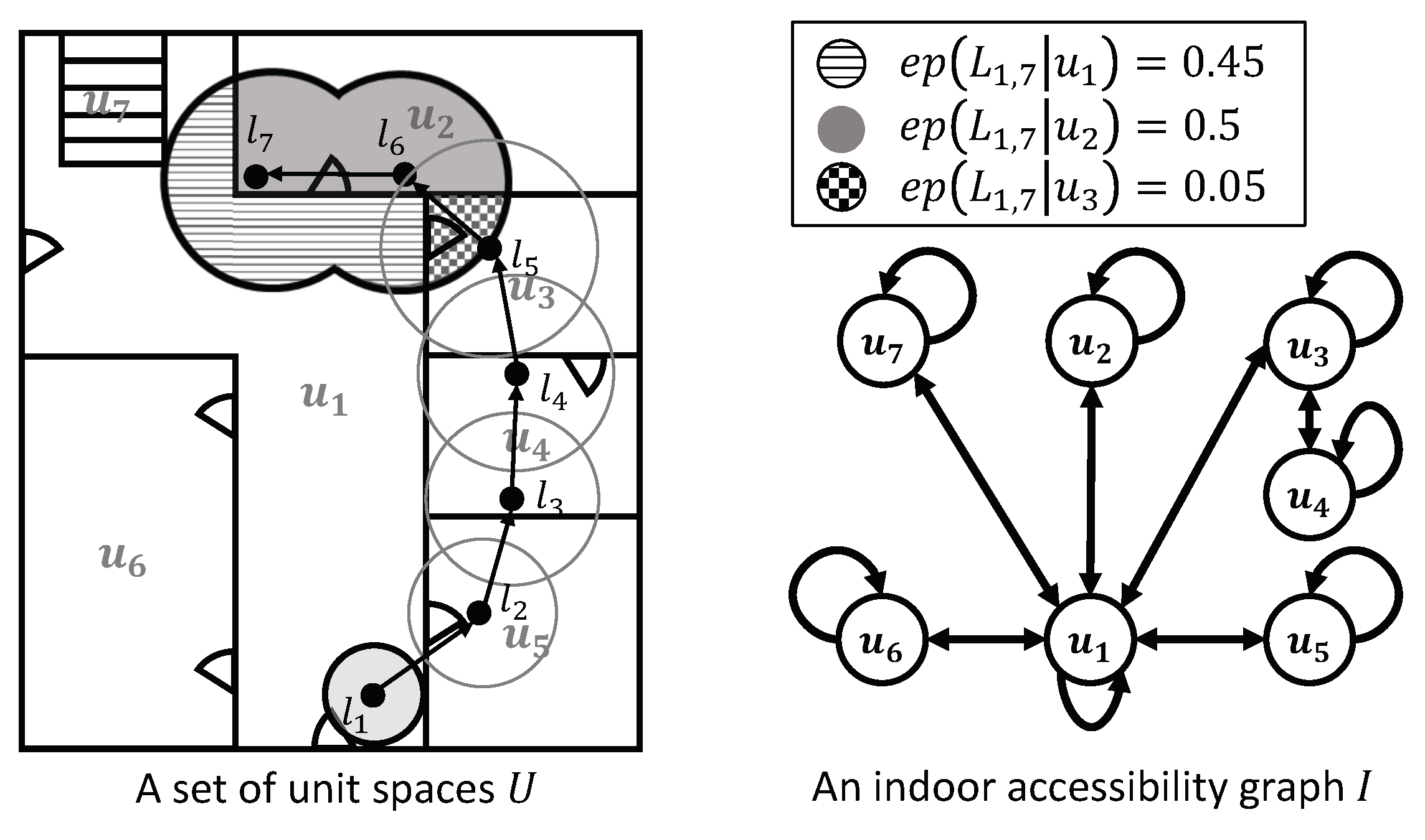
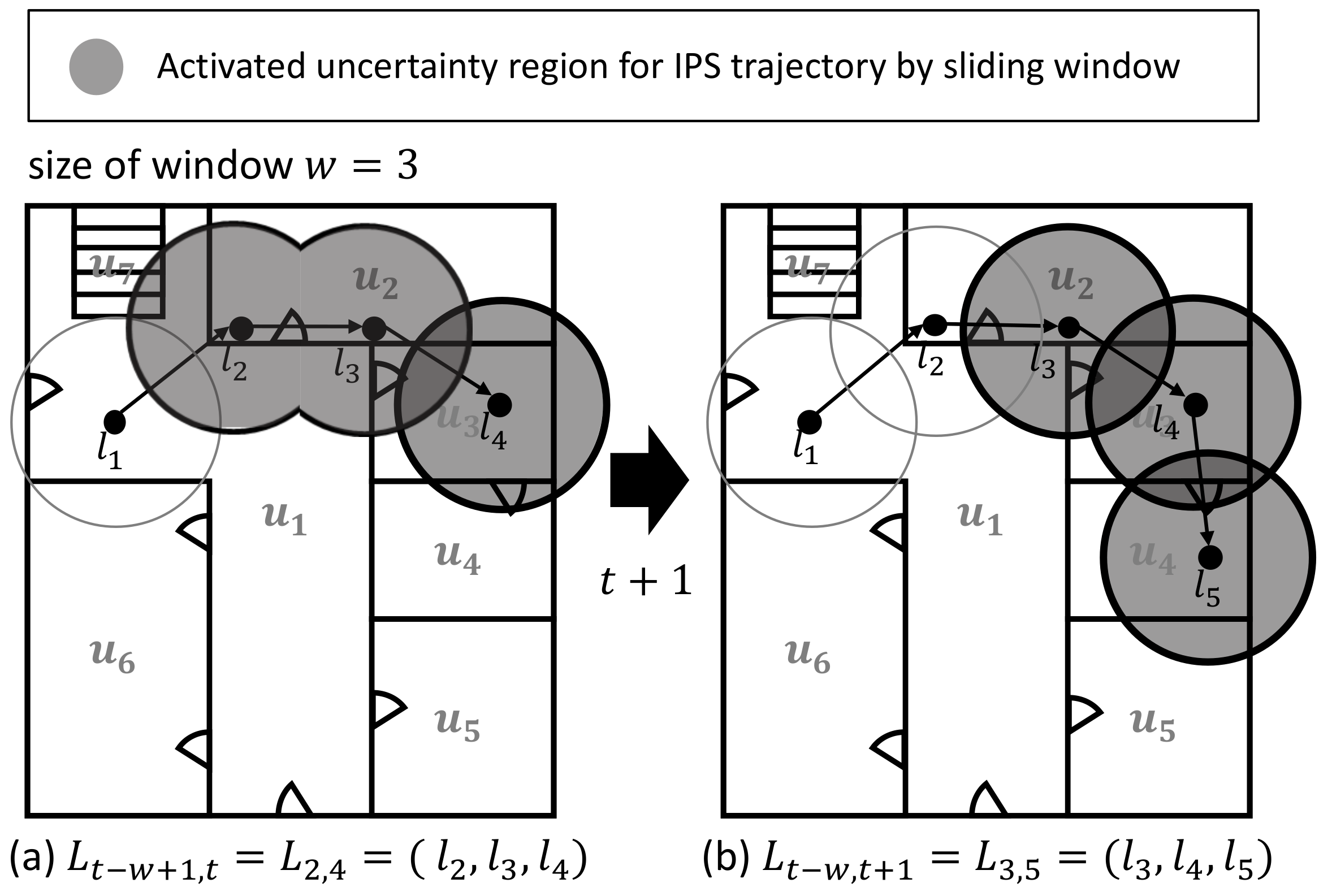
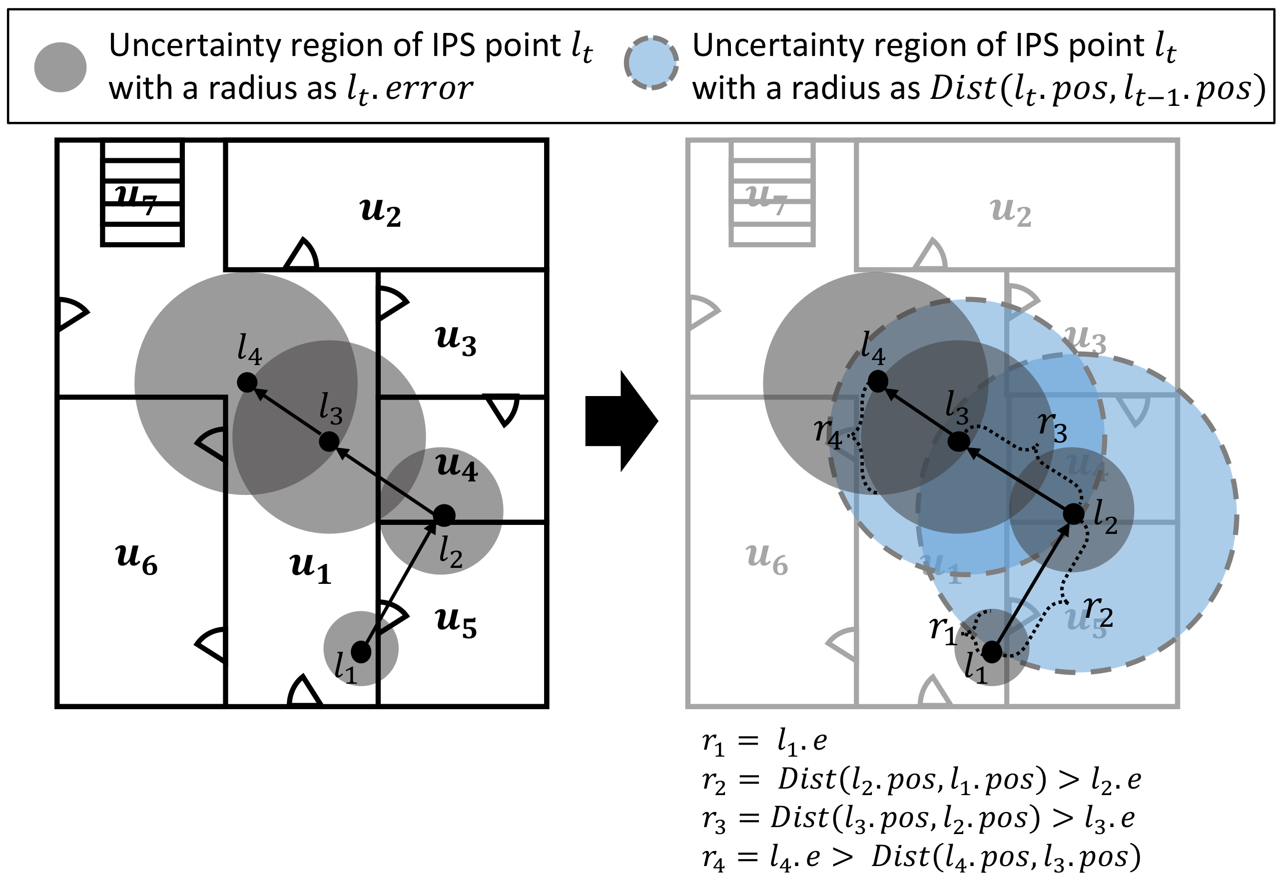
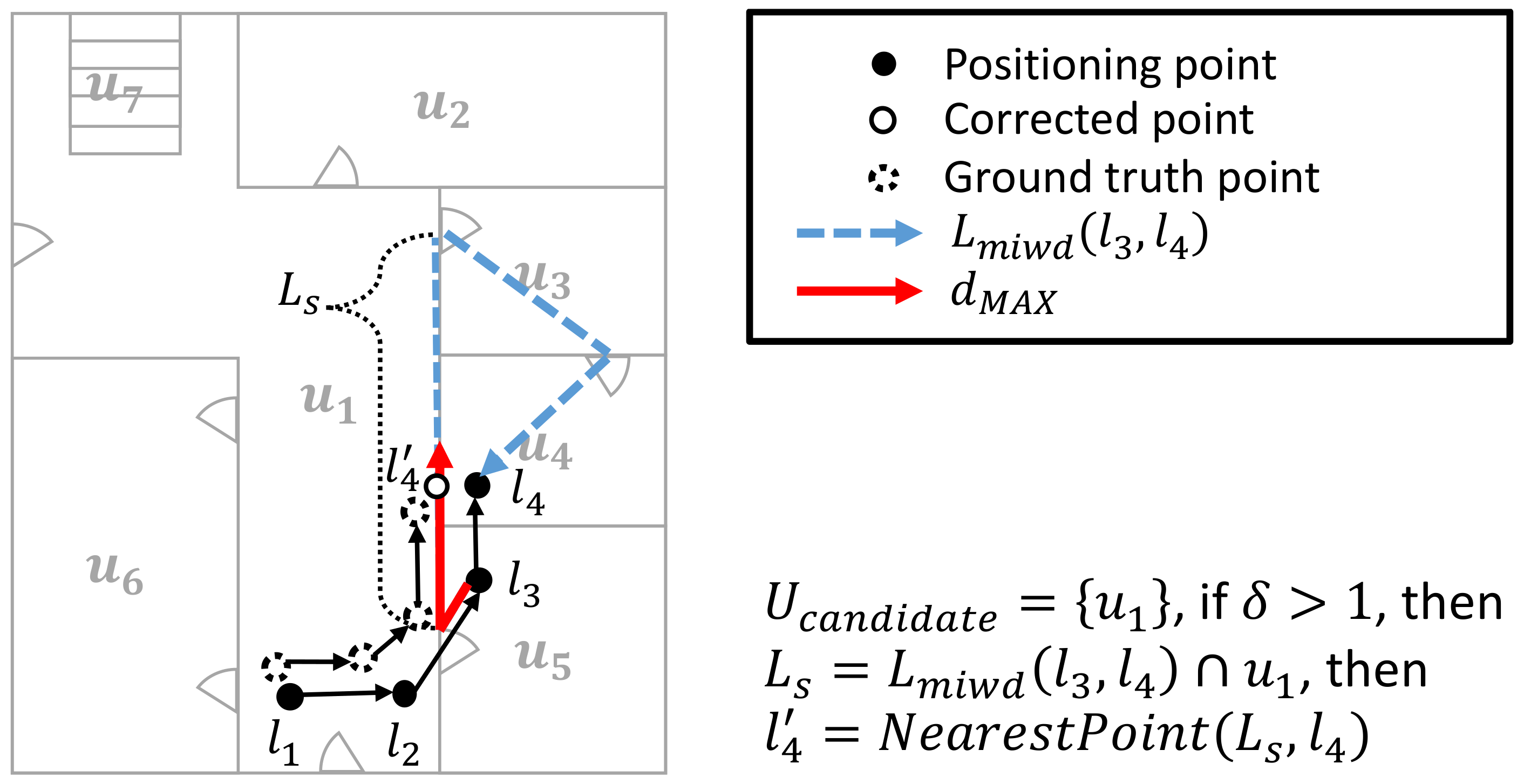
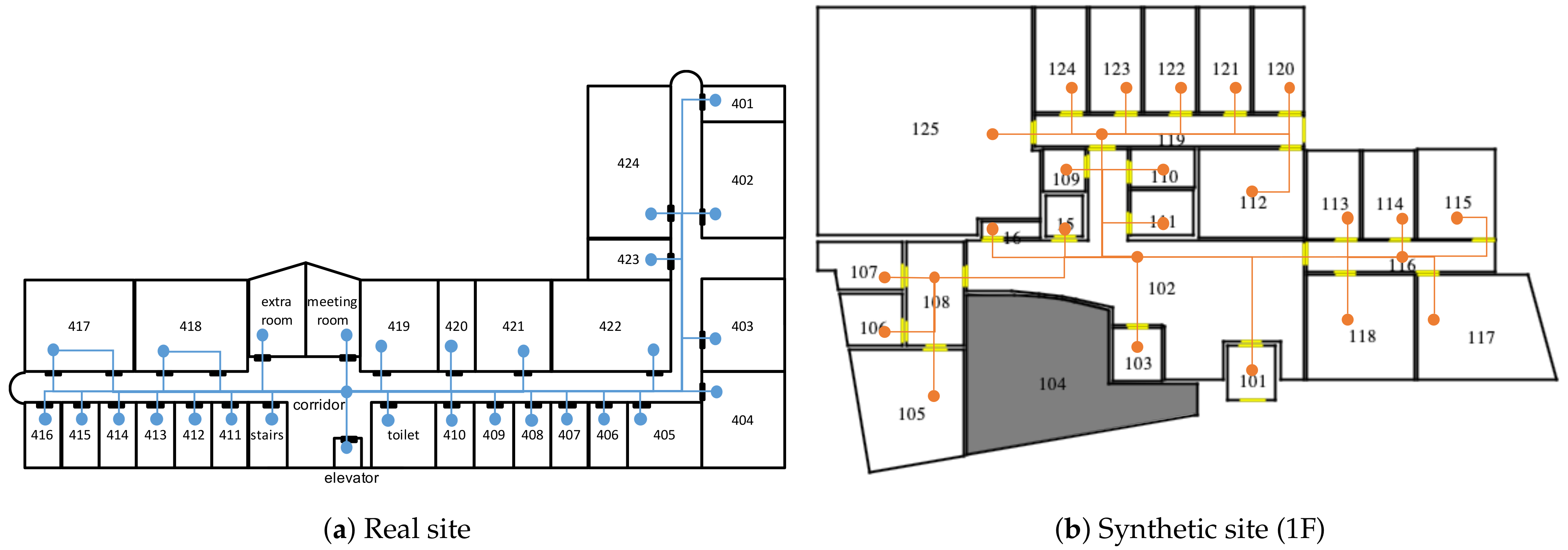
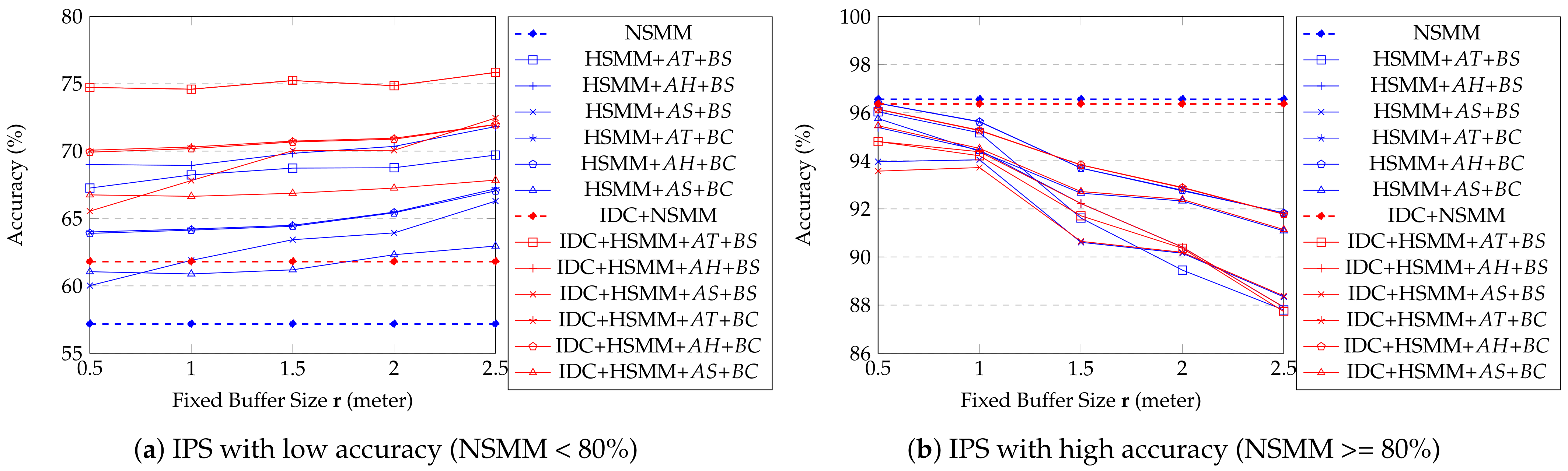
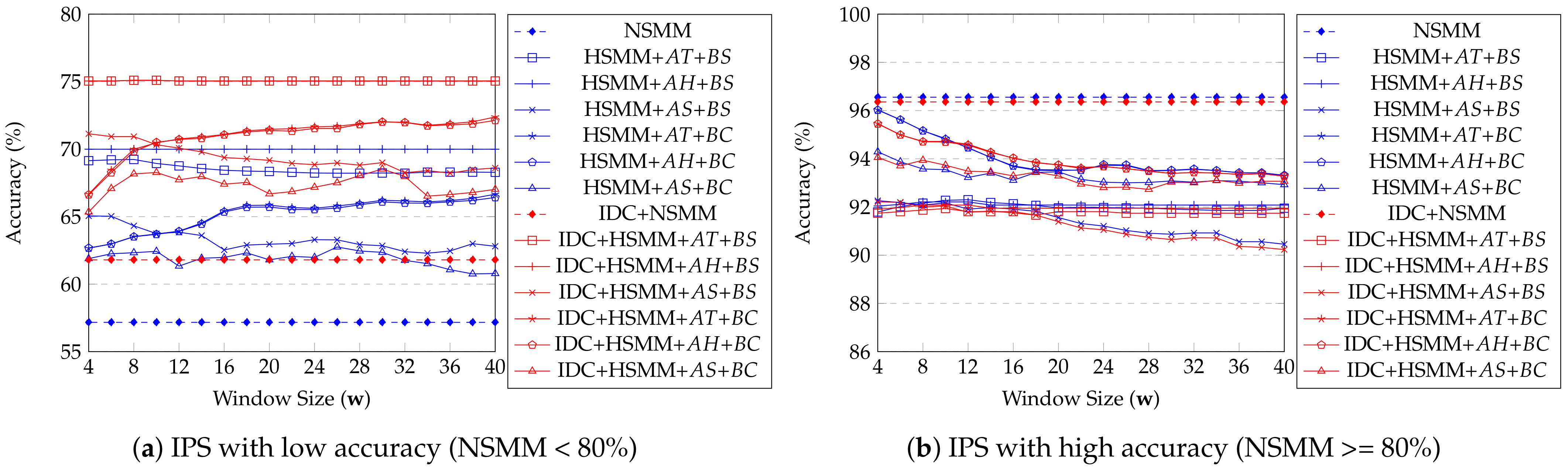
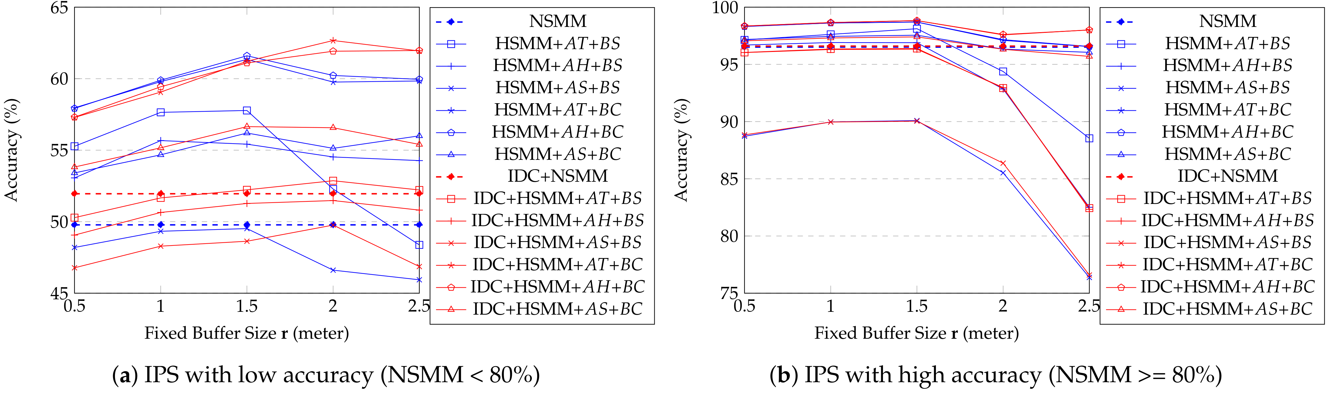
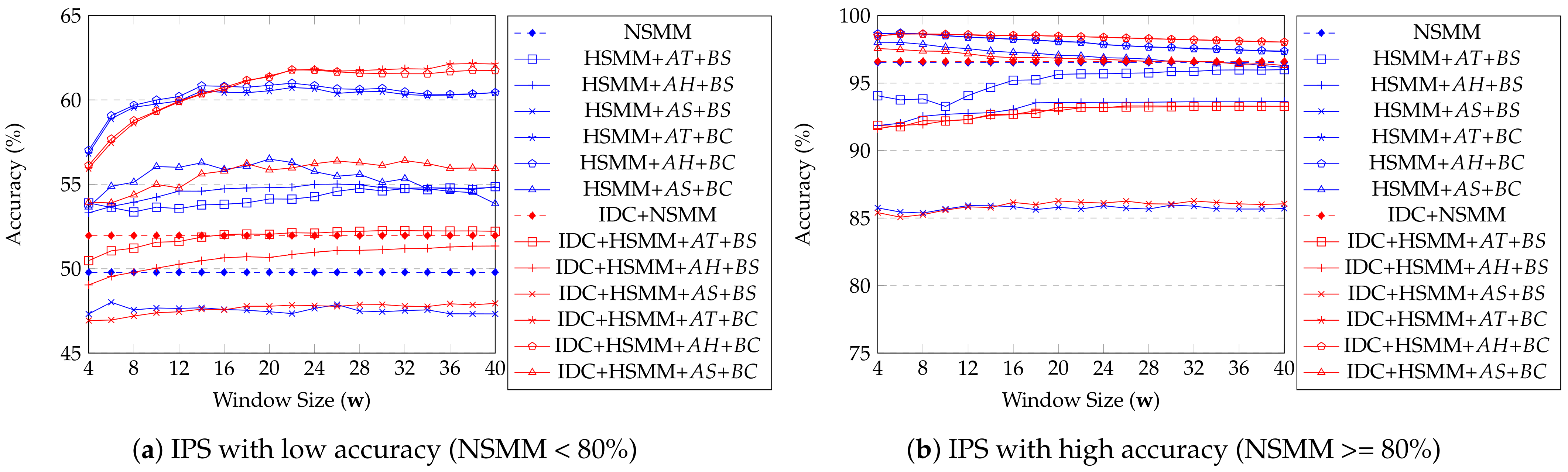
Table 1.
Summary of test site and data set.
| Features | Real Site | Synthetic Site |
|---|---|---|
| Number of unit spaces | 4F: 30 | 1F: 27, 2F: 33, 3F: 37 |
| Area (meters × meters) | 76.3 × 35.2 | 78.1 × 36.6 |
| Data format | OpenStreetMap XML | IFC file [78] |
| Data size (KBytes) | 51.2 | 43,142.5 |
| Number of trajectories | 35 | 180 |
| Number of points | 3093 | 13,436 |
| Sampling rates (seconds) | 1 | 1 |
| Average of error (meters) | - | 2.1350 |
| Variance of error (meters) | - | 1.9590 |
| Positioning algorithm | Hybrid | Trilateration |
Table 2.
Device information and experiment options for performance test.
| Features | Information |
|---|---|
| Device name | Xiaomi mi5 |
| Processor | Snapdragon 820 Quad-core Kryo 1.8 GHz |
| Memory | 3 GB LPDDR4 dual-channel RAM and 32 GB UFS 2.0 Flash |
| Size of window | 30 |
| Radius of buffer | 1.5 m |
| Setup methods | and |
Table 3.
Summary of experiment results.
| Experiment Site | Real Site | Simple Site | ||
|---|---|---|---|---|
| NSMM accuracy | <80% | >80% | <80% | >80% |
| Best USMM A matrix option | AT & AH | AT | AT | AT |
| Best USMM B matrix option | BS | BS | BC | BC |
| Best buffer size r | 2.5 | 0.5 | 2 | 1.5 |
| Best window size w | 8 & 10 | 2 | 38 | 8 |
| Performance of IDC | Well | Normal | Well | Normal |
Publisher’s Note: MDPI stays neutral with regard to jurisdictional claims in published maps and institutional affiliations. |
© 2021 by the authors. Licensee MDPI, Basel, Switzerland. This article is an open access article distributed under the terms and conditions of the Creative Commons Attribution (CC BY) license (https://creativecommons.org/licenses/by/4.0/).
Share and Cite
MDPI and ACS Style
Kim, T.; Kim, K.-S.; Li, K.-J. Improving Room-Level Location for Indoor Trajectory Tracking with Low IPS Accuracy. ISPRS Int. J. Geo-Inf. 2021, 10, 620. https://doi.org/10.3390/ijgi10090620
AMA Style
Kim T, Kim K-S, Li K-J. Improving Room-Level Location for Indoor Trajectory Tracking with Low IPS Accuracy. ISPRS International Journal of Geo-Information. 2021; 10(9):620. https://doi.org/10.3390/ijgi10090620
Chicago/Turabian StyleKim, Taehoon, Kyoung-Sook Kim, and Ki-Joune Li. 2021. "Improving Room-Level Location for Indoor Trajectory Tracking with Low IPS Accuracy" ISPRS International Journal of Geo-Information 10, no. 9: 620. https://doi.org/10.3390/ijgi10090620
Note that from the first issue of 2016, this journal uses article numbers instead of page numbers. See further details here.