Article

Random Forests with Bagging and Genetic Algorithms Coupled with Least Trimmed Squares Regression for Soil Moisture Deficit Using SMOS Satellite Soil Moisture

by
Prashant K. Srivastava
1,*,
George P. Petropoulos
2,
Rajendra Prasad
3 and
Dimitris Triantakonstantis
4
1
Remote Sensing Laboratory, Institute of Environment and Sustainable Development, Banaras Hindu University, Varanasi 221005, India
2
Department of Geography, Harokopio University of Athens, El. Venizelou 70, Kallithea, 17671 Athens, Greece
3
Department of Physics, Indian Institute of Technology, Banaras Hindu University, Varanasi 221005, India
4
Department of Soil Science of Athens, Institute of Soil and Water Resources, Hellenic Agricultural Organization “DIMITRA”, 1 Sofokli Venizelou, Lykovrisi, 14123 Attiki, Greece
*
Author to whom correspondence should be addressed.
ISPRS Int. J. Geo-Inf. 2021, 10(8), 507; https://doi.org/10.3390/ijgi10080507
Submission received: 28 April 2021 / Revised: 7 July 2021 / Accepted: 19 July 2021 / Published: 27 July 2021
(This article belongs to the Special Issue Integrating GIS and Remote Sensing in Soil Mapping and Modeling)

Abstract

:
Soil Moisture Deficit (SMD) is a key indicator of soil water content changes and is valuable to a variety of applications, such as weather and climate, natural disasters, agricultural water management, etc. Soil Moisture and Ocean Salinity (SMOS) is a dedicated mission focused on soil moisture retrieval and can be utilized for SMD estimation. In this study, the use of soil moisture derived from SMOS has been provided for the estimation of SMD at a catchment scale. Several approaches for the estimation of SMD are implemented herein, using algorithms such as Random Forests (RF) and Genetic Algorithms coupled with Least Trimmed Squares (GALTS) regression. The results show that for SMD estimation, the RF algorithm performed best as compared to the GALTS, with Root Mean Square Errors (RMSEs) of 0.021 and 0.024, respectively. All in all, our study findings can provide important assistance towards developing the accuracy and applicability of remote sensing-based products for operational use.

1. Introduction

Soil moisture is of key importance in numerous fields from weather, climate, agricultural to hydrological sciences [1]. It is also considered as an Essential Climatic Variable (ECV) in 2010 [2,3,4,5]. To cater the needs of hydro-meteorologist and remote sensing community one after the other, two dedicated global space satellites have been launched to offer measurements of the soil moisture in the globe: (a) the Soil Moisture and Ocean Salinity (SMOS) mission, launched by the European Space Agency in November 2009, and (b) the Soil Moisture Active Passive (SMAP), launched in 2016 by the National Aeronautics and Space Administration (NASA) [6]. In agricultural applications, the estimation of soil moisture from the Earth’s surface is important for a successful management of soil water content and irrigation scheduling. At first, soil moisture can be assessed by utilizing the in-situ probes, an approach which is adequate with the local or point based applications. However, retrieving large scale soil moisture under vegetation conditions is a challenging task because of large spatial variability and heterogeneity in the crop types [7,8]. Different crop types are characterized by different moisture contents, which make many practical applications difficult [9]. Therefore, alternate approaches are needed for an effective agricultural water management [10].
In hydrology, a common soil moisture indicator is the soil moisture deficit (SMD) or depletion, which is directly related to the ratio between actual and potential evapotranspiration (PE) [11,12,13]. It shows the water required to lift the soil-water content of the crop root zone to field capacity [14,15]. SMD is a vital indicator of water availability, representing the constraint variable in crop yields. The moisture deficit impact on agricultural yield has been examined at multiple scales regarding different soil management practices [16,17,18]. It is important for crops monitoring because it has a strong impact in sowing, harvesting and finally in crop yield. Timely information of SMD is useful in crop insurance practices and to protect equity against natural disasters such as drought, floods and other socio-economic factors [19]. When a drought occurs, a high value of SMD is generally evident for a prolonged time, while during a flood, SMD is very low [20,21]. There have been a number of studies on the Probability Distribution Model (PDM) [22,23] and their results could be used as a suitable option for SMD generation using the minimal datasets, such as rainfall, evapotranspiration and discharge information. Recently, a few studies by Srivastava et al., 2013, 2014 [3,10] indicated that the soil moisture is strongly linked with the SMD and could be used for estimating this variable.
Some recent research has also indicated significant non-linear relationships between the SMD and soil moisture. In this regard, genetic programming (GP) [24] and RFsregression [25] can be used as non-linear techniques for modeling SMD by using soil moisture estimated from SMOS satellite. Among machine learning, the GP and RFs are evolutionary algorithms that can be used for the estimation of SMD. It is inspired by the biological evolution to find computer programs that perform a user-defined task, generally based on chromosome crossing over for getting a better offspring [26]. The RFs algorithm is a non-parametric technique that is capable of synthesizing regression functions based on discrete or continuous datasets in the field of remote sensing [27,28,29]. RFs is a strong model in regard to the outliers and can be executed efficiently on large datasets for the regression problems [30]. The RFRmodel’s robustness over Support Vector Regression (SVR) and Artificial Neural Network Regression (ANNR) has been demonstrated wheat crop biomass estimation [31]. Soil mapping was performed by utilizing an RFs model in Africa with relatively accurate results. External parameter orthogonalization, coupled with RFs, SVM, partial least squares regression and ANN models, was applied on a larger soil database and satisfactory results were obtained. With the advancement in machine learning models, the Genetic Algorithm coupled with Least Trimmed Squares (GALTS) [32] has been developed, which uses a small number of trials to achieve the objective functions; as a result, it reduces the variance and biases in the datasets.
To our knowledge, a very small number of studies have focused on comparing the use of RFs and GP for SMD estimation. In viewof the above, in this study, a first-time comprehensive evaluation of the use of the RFs and GALTS algorithms are explored in retrieving the SMD using SMOS data for soil moisture information. To validate the model, the benchmark SMD obtained using the PDM model has been used. Before using the output, i.e., SMD, a rigorous sensitivity and uncertainty analysis of PDM has been performed using the state-of-the-art Generalized Likelihood Uncertainty Estimation [33]. The knowledge gained from this study can potentially assist in evaluating the relation between the rainfall runoff model and satellite soil moisture. Furthermore, exploring this relationship is an essential step to help further developing the accuracy and applicability of such products for operational uses exploiting EO technology.

2. Study area and Datasets
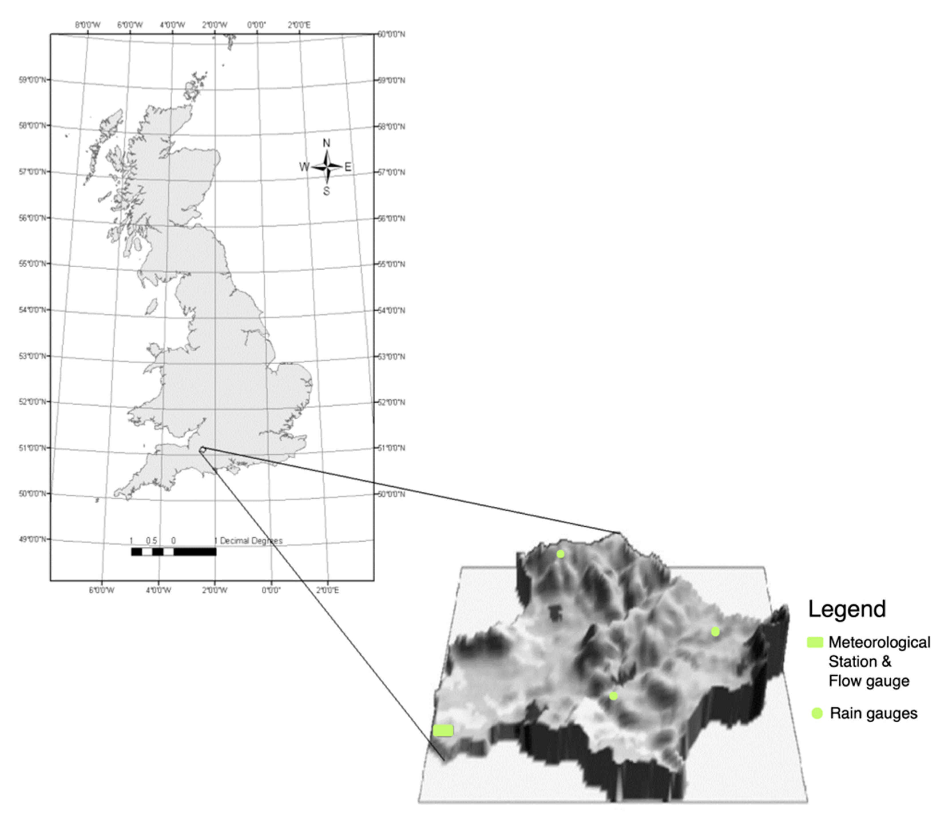
2.1. Study Area

The Brue catchment (total area 135.5 km2) located in the south-west of England is chosen as the study area (Figure 1). The lowland wet grassland of the catchment forms part of the unique landscape of the Somerset Levels and Moors and the region is internationally and nationally designated for its conservation and landscape value. The other minor cover types found in the catchment are forest and urban areas. The area is characterized by a non-complex topography area for the most part, with most of the catchment area covered by agricultural land (95.22%), with a small number of forest patches (3.12%) and urban areas (1.66%). In the Brue catchment, the distribution of soil indicates that most of the area is composed of a clayey type (49%) of soil followed by coarse loam (29%) and silt (21%). The selected study area has been used previously in many studies and equipped with maintained meteorological and flow station by British Atmospheric Data Centre and Environment Agency, respectively [34,35,36,37]. The whole terrain comes under topography, with no steep slopes and with an average altitude of 105 m AMSL.

2.2. Satellite Data

The SMOS satellite contains the MIRAS instrument—a dual polarized 2D interferometer that operates at a frequency of 1.4 GHz (L-band) [38], launched jointly by the European Space Agency (ESA), the National Centre for Space Studies (CNES-Centre National d’Etudes Spatiales) and the Industrial Technological Development Centre (CDTI–Centro para el Desarrollo Technológico Industrial). The radiometric resolution of the instrument is ~40 km with the soil moisture retrieval unit in m3 m−3 (i.e., volumetric). In the current study, Level 2 SMOS soil moisture products are used, generated by the SMOS level 2 processor. Acquisition of all the datasets started from February 2011 to January 2012. Soil moisture or surface salinity consist of Level 2 products swath-based maps computed from Level 1c products. The conversion from Level 1c brightness temperatures to Level 2 maps includes a first step to mitigate the impact of Faraday rotation, Sun/Moon/galactic glint, atmospheric attenuation, etc. SMOS acquires data in Icosahedral Snyder Equal Area projection (ISEA 4H9 grid) [39]. Each point (or node) of this grid is known as a DGG that has fixed coordinates and is assigned with an identificator, “DGG Id.” For the development of the model, the SMOS pixel with its centroid over the catchment is extracted and considered for the subsequent analysis. The Beam (v 4.9) (developed under ESA Envisat project by Brockmann Consult GmBh, Germany) open-source software package with SMOS 2.1.3 plugin was used for the extraction. The ascending SMOS data products are selected in the catchment area to minimize the variables influencing soil moisture retrieval, such as vertical soil-vegetation temperature gradients.

3. Probability Distributed Model (PDM)

The PDM model from CEH Wallingford [40] is used as a rainfall runoff simulation model in this study for SMD estimation, as it can calculate soil moisture in the system with suitable time step and data inputs required for use in a water resources assessment. In this study, the lumped rainfall-runoff models called as PDM (Probability Distributed Model) has been used for benchmarking SMD estimation using ground-based datasets. Daily datasets from February 2011 to January 2012 has been used for the model calibration and validation. The PDM model is a fairly general conceptual rainfall-runoff model which transforms rainfall and evaporation data to flow at the catchment outlet and is well tested [41]. It has evolved as a toolkit of model functions that together constitute a lumped rainfall-runoff model capable of representing a variety of catchment-scale hydrological behaviors. The model formulations are adjusted for automatic parameter assessment. For real-time flow forecasting applications, the PDM model is complemented by updating methods based on error prediction and state-correction approaches [36]. The PDM model require three main inputs—evapotranspiration, rainfall and river flow—and the output products are flow and SMD [42]. The SMD is produced to describe the effect of drying on the catchment area on the actual evapotranspiration (ET). The SMD routine in PDM is based on [40]:
E i E i = 1 S max S ( t ) S max b e
where E i E i is the ratio of actual ET to potential ET; S max S ( t ) is the Soil Moisture Deficit; be is an exponent in the actual evaporation function; S max is the total available storage; and S ( t ) is storage at a particular time t. The Sensitivity analysis (SA) and uncertainty analysis (UA) of the PDM model over the Brue catchment are given in detail by [33]. From the study, it can be concluded that PDM can be used for SMD estimation with less uncertainty, and therefore, it can be used as reference data.

4. Random Forests and Genetic Algorithm Coupled with Least Trimmed Squares (GALTS)

R programming language is used for all the algorithms implementation, which is open-source software. The techniques involve RFsand Genetic Algorithm coupled with Least Trimmed Squares (GALTS) regression for SMD estimation.

4.1. Genetic Algorithm Using Least Trimmed Square (GALTS)

GALTS draws random candidate solutions (or chromosomes) for which search methods are appropriate for use in nonlinear or non-differentiable optimization problems [32]. Genetic Algorithms (GAs) perform a parallel search to cope with the local optima problem. Offspring are selected based on their survival in subsequent generations. However, the minimization of the objective function is a complicated problem in GAs. The authors of one paper [43] developed a method for regression parameter assessment using a Least Trimmed Square (LTS) calculation in a broad dataset. It is an appropriate algorithm because it has been successfully demonstrated in several test beds in the literature, including studies similar to ours, and references have been provided. The purpose of this study is not to perform a comparison between algorithms, which could be a very interesting direction to pursue in a follow-up paper. Some researchers also used least median of squares (LMS) regression for outlier detection, but its convergence rate is slow [43]. On the contrary, LTS has the same breakdown point as LMS, but the convergencerate is quicker than LMS. The objective function of the LTS regression is defined as:
min β i = 1 h r i 2
where r i 2 is the ith ordered squared residual and h is a custom integer, which is approximately n/2.

4.2. Random Forests

RFs, which was proposed by [30], is a machine learning algorithm which adds an additional layer of randomness to bagging and fits regression trees to random subsets of the input data [44]. The main advantage with RFs is that it is designed to produce accurate predictions that do not overfit the data [30], and differs from bootstrap in constructing the multiple trees. In this study, bagging is used in tandem with random feature selection. RFs for regression are produced by growing trees depending on a random vector Θ, such that the tree predictor h(x,Θ) takes on numerical values as opposed to class labels with assumption that that the training set is independently drawn from the distribution of the random vector Y, X. The mean-squared generalization error for any numerical predictor h(x) is given by Equation (3):
E X , Y ( Y h ( X ) ) 2
The RFpredictor is formed by taking the average over k of the trees {h(xk)} as:
E X , Y ( Y a v k h ( X , Θ k ) ) 2 E X , Y ( Y E Θ h ( X , Θ ) ) 2
The forest trees can be simplified by using the term P E ( t r e e ) , where it can be defined as Equation (5):
P E ( t r e e ) = E Θ E X , Y ( Y h ( X , Θ ) ) 2
It can be used for estimating P E ( f o r e s t ) (Equation (6)):
P E ( f o r e s t ) ρ ¯ P E ( t r e e )
P E ( f o r e s t ) can be summarized by Equation (7):
P E ( f o r e s t ) = E X , Y [ E Θ ( Y h ( X , Θ ) ] 2 = E Θ E Θ E X , Y ( Y h ( X , Θ ) ) ( Y h ( X , Θ ) )
The term on the right in (Equation (7)) is a covariance and can be written as:
E Θ E Θ ( ρ ( Θ , Θ ) s d ( Θ ) s d ( Θ ) )
where s d ( Θ ) = E X , Y ( Y h ( X , Θ ) ) 2 ; the weighted correlation can be defined as (Equation (8)):
ρ ¯ = E Θ E Θ ( ρ ( Θ , Θ ) s d ( Θ ) s d ( Θ ) ) / E Θ s d ( Θ ) ) 2
Then, this condition will follow (Equation (9)):
P E ( f o r e s t ) ρ ¯ ( E Θ s d ( Θ ) ) 2 ρ ¯ P E ( t r e e )
The requirements for accurate RFs are a low correlation between residuals and low error trees. The RFs decreases the average error of the trees employed by the factor ρ ¯ .

5. Performance Evaluation

The estimated SMD of the RFs and GALTS models are compared against the locally estimated SMD through PDM. This is performed in terms of the correlation (r), the Root Mean Square Error (RMSE) and the absolute bias (Bias). The bias measures the over- and underestimation of the model output (Equation (10)). The r can be calculated by using Equation (11), while the RMSE can be estimated by using Equation (12):
B i a s = [ ( y ¯ x ¯ ) ]
r = n x y x y n x 2 x 2 n y 2 y 2
R M S E = 1 n i = 1 n y i x i 2
where xi i is the observed flow, yi is is the simulated flow and x ¯ is the mean.

6. Results and Discussion

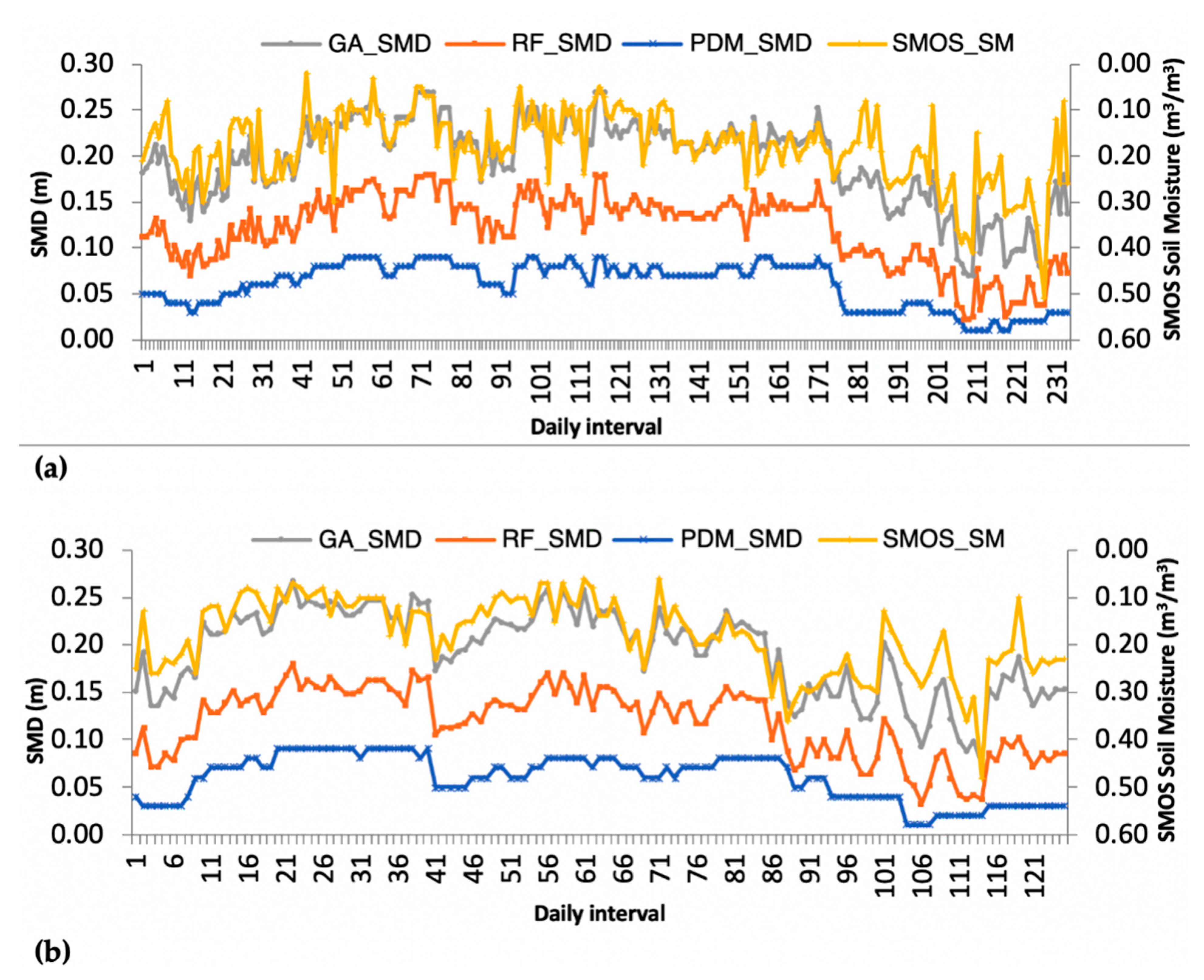
6.1. SMD and Soil Moisture Temporal Variations

The temporal pattern between SMOS soil moisture, PDM SMD, RFs and GALTS simulated SMD during calibration and validation is represented through Figure 2. The plots show a high level of temporal variability over the entire monitoring cycle, with a daily step beginning from the first day of January. The distinctive dry periods can be demonstrated, when a distinctive rise in the SMD occurred in the plot. During the period, the trend and pattern in the datasets are very close to the one estimated by the PDM. In general, soil moisture retrieved by SMOS is highly responsive with significant fluctuations over the whole period even to the small variations in SMD. During December and January, a very high value of soil moisture is reported. Over April–May to August–September, rising temperatures and high evaporation cause the soil to dry out, resulting in a rise in SMD values. Increasing temperature caused a substantial SMD development prominent from April to the beginning of August (normally, the driest and warmest months of the year). Drying out follows an exponential decay and an inverse relation can be seen with SMOS soil moisture. According to soil moisture analysis, the wettest months are November and December, while the driest months are March and May. Soil moisture is poor during the winter and near field capacity by mid-April.

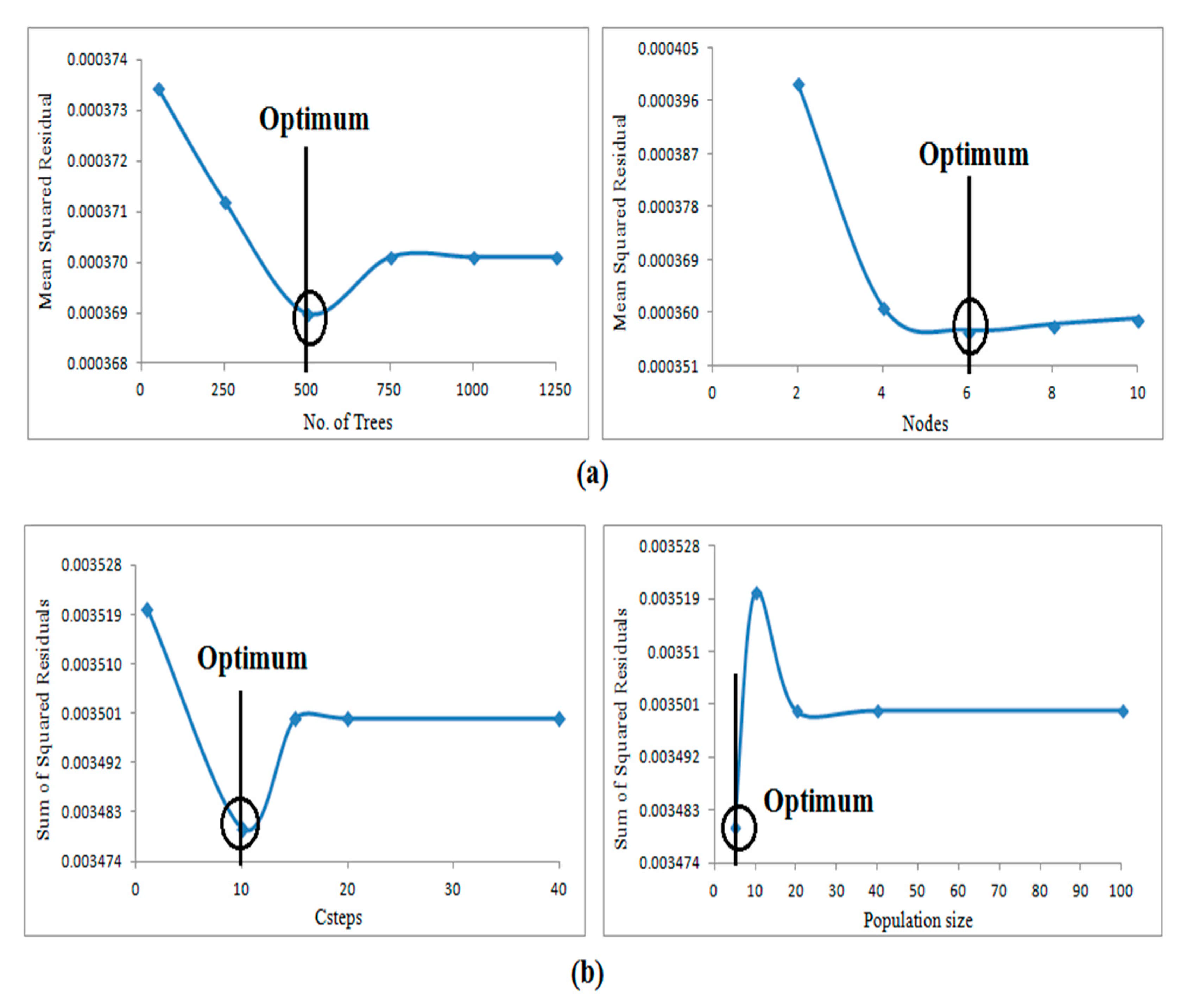
6.2. Optimisation of RFs and GALTSAlgorithms

For reliable results, the RFs and GALTS techniques must be optimized, which necessitates a preliminary review of parameters before using them for the final prediction (Figure 3). For RFs, initially, we started with a very small number of trees (around 50) and measured the performance of the technique with respect to the measured SMD. This process was repeated up to a total of 1250 number of forest trees. The mean squared sum of residual is used as an objective function for optimizing the number of trees. For any artificial intelligence technique, this form of trial-and-error approach is widely used to select the right parameters [42]. A similar approach is used for optimizing the number of nodes in RFs. After all the analysis, the optimum values of parameters are obtained as 500 with respect to number of trees and 6 for the number of nodes in the RFs algorithm.
For optimization of GALTS, two important parameters, i.e., Csteps and population size, are taken into account. As recommended by [43], the sum of squared residuals is taken as an objective function for the optimization of parameters. In case of Csteps, initially, we began with 1 and gradually increase it up to total 40 numbers of Csteps. After a comparison with the SMD, a total of 10 Csteps were found to be appropriate for GALTS. After repeating the procedure with the population sizes from 5–100, a population size of 5 is found optimum for SMD prediction.

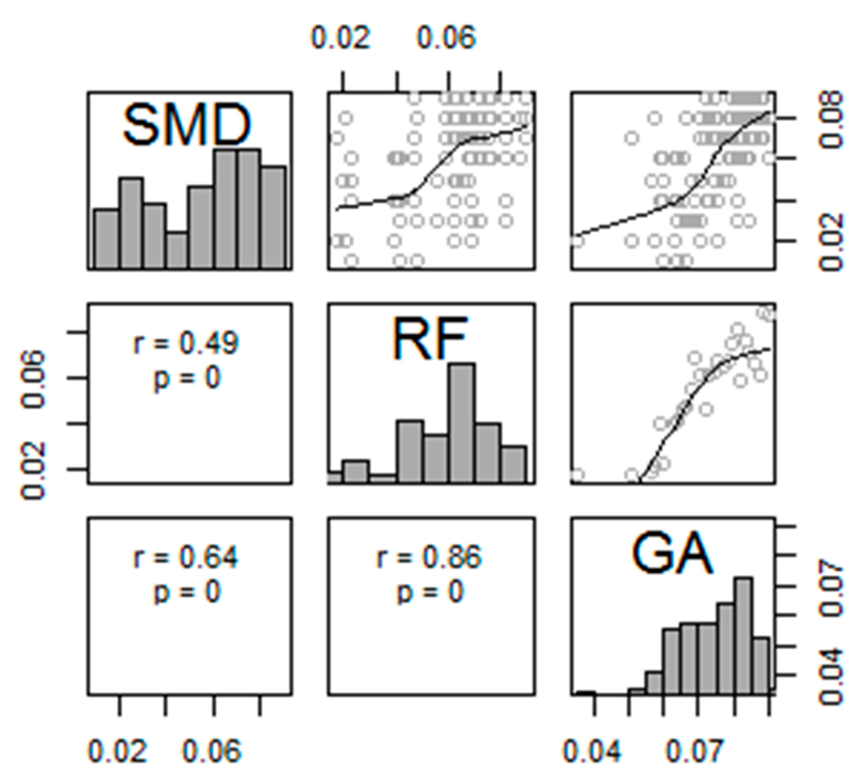
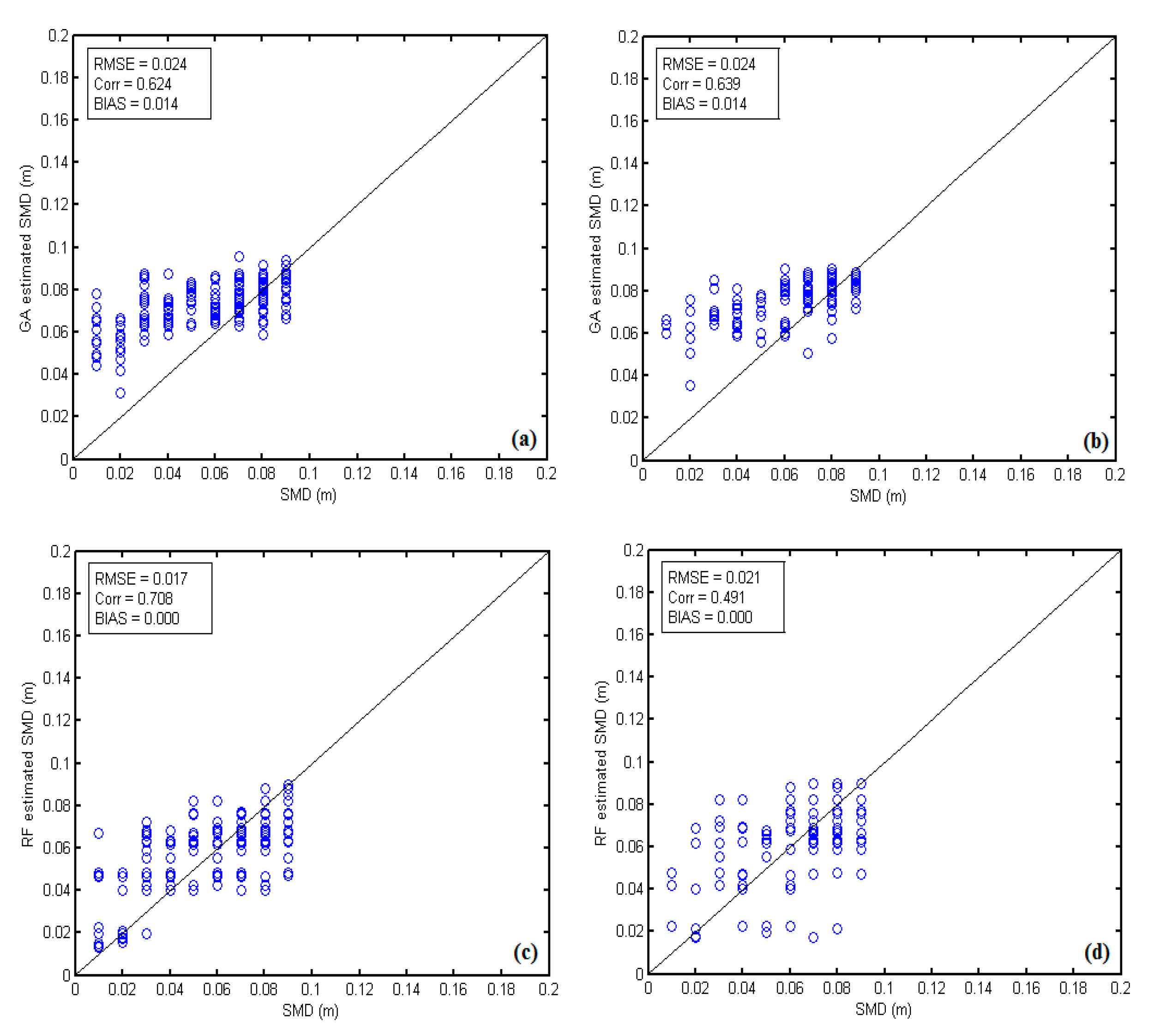
6.3. Performances of RFs and GALTS for SMD Prediction

For SMD prediction using the SMOS soil moisture, RFs and GALTS methods are used, while scatter plots depicting the output of various approaches in terms of correlations are given in Figure 4. For developing an appropriate algorithm, the calibration and validation datasets are split into two groups first. Two-thirds of the data from each month is used for calibration, while the other third is used for validation, ensuring that all calibration and validation data are indicative of both seasons. After deriving the relationships, the validation results are used to test the algorithms. The notable things observed in the validation correlation plot are some lower correlations of RFs-simulated SMD, while the correlation of GA-simulated SMD indicate a higher value with the PDM SMD. The best correlation statistics are obtained GALTS with a value of 0.64, followed by a value of 0.49 with RFs-estimated SMD.
The scatter plots produced from all the approaches at the calibration and validation phases are depicted through Figure 5. Looking at the values of the Bias, the RFs performed well with the least overestimation and low RMSE, although the value of r is lesser than GALTS. Higher bias and RMSE values obtained by GALTS indicated that the simulated results are overestimated as compared with the RFs. The analysis indicates that the outcome of the RFs can be used for estimation of SMD from SMOS soil moisture. Some binning can be seen in the plot, which could be due to saturation of the SMD values predicted during the particular time period. Furthermore, as PDM is a conceptual model based on water balance, when there are small changes in soil moisture in the region, this will lead to a very negligible variation in the SMD, which cannot be clearly demarcated in the scatter plots.

6.4. Other Relevant Studies

In another study, to estimate the SMD [3], soil moisture was estimated from certain algorithms, such as Single channel calculation (SCA). It was found that the inclusion of a physics-based equation for soil moisture retrieval and the incorporation of linear and non-linear models improves the SMD prediction. Moreover, better accuracy is produced with locally calibrated roughness parameters rather than default global values, because they represent the conditions more precisely.
In other research [10], the SMD was estimated by using soil moisture by SMOS and WRF-NOAH LSM as well. Four data fusion models were evaluated: Linear Weighted Algorithm (LWA), Multiple Linear Regression (MLR), Kalman Filter (KF) and Artificial Neural Network (ANN). The LWA method utilizes combinations between soil moisture products. The MLR method uses as a dependent variable the SMD produced by the Probability Distributed Model and as predictors the SMOS and WRF-NOAH LSM. The validation of the different models against SMD produced by the Probability Distributed Model was achieved using ground-based observations. All the data fusion algorithms enhance the information quality and, subsequently, they are appropriate for SMD calculation for hydrological applications. More specifically, the analysis indicated a higher suitability of ANN and KF for data fusion than the LWA or MLR technique. These methods can be used for the data fusion, giving profitable information on the appropriateness of SMOS and WRF-NOAH LSM for SMD calculation.
To assess the suitability of WRF for SMD calculation, ref. [45] used three domains with spatial resolutions of 81 km, 27 km and 9 km. The best domain (Innermost WRF domain of 9 km) was used for estimating the soil moisture deficit (SMD). Two approaches were used in this study. The first method is based on a continuous time series analytical relationship between WRF soil moisture and the SMD, while the second is centered on the effect of vegetation cover on SMD retrieval, represented in terms of growing and non-growing seasons. The results indicated that both approaches could be useful for soil moisture and SMD calculation at the catchment level.
Concluding the relevant studies of SMD estimation, ref. [18] used a process-based Soil and Water Assessment Tool (SWAT) model to simulate the multi-annual fluctuations of soil moisture anomalies (deficits or excesses). For two potential horizons, i.e.,2021–2050 and 2071–2100, the analysis used an ensemble of nine bias-corrected EURO-CORDEX forecasts under two Representative Concentration Pathways: RCP4.5 and 8.5. SWAT, which collects significant SMD and soil moisture excess episodes for various crops, according to the findings. The severity of soil moisture deficits increased for spring cereals, potato and maize. Furthermore, soil moisture excesses were more dependent on RCP and potential horizon selection for potato and maize.
The proposed method could be very useful for ungauged catchments, with as thelimitations that it is developed in an environment that is influenced by a temperate oceanic climate, and hence, it may not be suitable for tropical climates. New optimization parameters and coefficients will be required if the method is implemented in tropical climates or other types of climates. In this case, catchment is very small, so even three gauges are sufficient to develop an appropriate model; however, for larger catchments, a dense gauge networks may be needed for developing some suitable models for SMD prediction.

7. Conclusions

SMD is an integral component for most of the hydrological models and needed for designing appropriate routing schemes. The results indicate that the SMOS soil moisture has proven its importance in hydrological sciences and can be used for the prediction of SMD. The findings of this research show that satellite soil moisture, such as from SMOS, can be used for SMD estimation using sophisticated techniques, such as RFs and GALTS. Performance indices indicated that the RFs performed well with a low bias and small RMSE, although the value of the correlation is lowerthan GALTS. Higher bias and RMSE values obtained by GALTS indicated that the simulated results are overestimated as compared to the RFs. The overall performance of RFs showed that using SMOS soil moisture data, the RFs can be used to estimate SMD. However, more work is needed in the future to reduce the biases in the predictions, as some over estimation is evident in the SMD estimation. Thus, in the future, attempts will be made on the bias correction schemes, so that an operational forecast can be provided for SMD. Moreover, in the future, SMD estimation will be done in other geographical areas as well, so that valuable information and insights can be gathered using other promising satellites such as the Soil Moisture Active Passive satellite (SMAP).

Author Contributions

Conceptualization, Prashant K. Srivastava; Data curation, Prashant K. Srivastava; Formal analysis, Prashant K. Srivastava; Investigation, Prashant K. Srivastava and George P. Petropoulos; Method-ology, Prashant K. Srivastava and George P. Petropoulos; Resources, George P. Petropoulos and Dimitris Triantakonstantis; Visualization, Prashant K. Srivastava, George P. Petropoulos, Rajendra Prasad; Writing—original draft, Prashant K. Srivastava, Dimitris Triantakonstantis; Writing—review & editing, Prashant K. Srivastava, George P. Petropoulos, Dimitris Triantakonstantis and Rajendra Prasad All authors have read and agreed to the published version of the manuscript.

Funding

This research received no external funding.

Institutional Review Board Statement

Not Applicable.

Informed Consent Statement

Not Applicable.

Data Availability Statement

SMOS data used in this study can be downloaded from ESA, while ground based Brue catchment datasets can be obtained from British Atmospheric Data Centre on request.

Acknowledgments

The Commonwealth Scholarship Commission, British Council, United Kingdom, and Ministry of Human Resource Development, Government of India provided the required assistance and funding for this study, which the authors gratefully acknowledge. The authors are grateful to the European Space Agency, who provided the SMOS data. Moreover, the authors would like to thank the British Atmospheric Data Centre for its assistance with the ground observation information. Lastly, special thanks to Yann Kerr, Director, CESBIO, France, for providing the training on the SMOS datasets to the first author.

Conflicts of Interest

The authors declare no conflict of interest.

References

  1. Tsatsaris, A.; Kalogeropoulos, K.; Stathopoulos, N.; Louka, P.; Tsanakas, K.; Tsesmelis, D.E.; Krassanakis, V.; Petropoulos, G.P.; Pappas, V.; Chalkias, C. Geoinformation Technologies in Support of Environmental Hazards Monitoring under Climate Change: An Extensive Review. ISPRS Int. J. Geo-Inf. 2021, 10, 94. [Google Scholar] [CrossRef]
  2. Smith, J.M. Mathematical Modelling and Digital Simulation for Engineers and Scientists; John Wiley & Sons, Inc.: Hoboken, NJ, USA, 1986. [Google Scholar]
  3. Srivastava, P.K.; Han, D.; Rico-Ramirez, M.A.; O’Neill, P.; Islam, T.; Gupta, M. Assessment of SMOS soil moisture retrieval parameters using tau–omega algorithms for soil moisture deficit estimation. J. Hydrol. 2014, 519, 574–587. [Google Scholar] [CrossRef] [Green Version]
  4. Petropoulos, G.P.; McCalmont, J.P. An operational in-situ soil moisture and soil temperature monitoring network for west Wales, UK: The WSMN network. Sensors 2017, 17, 1481–1491. [Google Scholar] [CrossRef] [Green Version]
  5. Maurya, S.; Srivastava, P.K.; Yaduvanshi, A.; Petropoulos, G.P.; Zhuo, L.; Mall, R.K. Future projections of soil erosion using Coupled Model Intercomparison Project and Earth Observation datasets. J. Hydrol. 2021, 594. [Google Scholar] [CrossRef]
  6. Petropoulos, G.P.; Sandric, I.; Hristopulos, D.; Carlson, T.N. Evaporative fluxes and Surface Soil Moisture Retrievals in a Mediterranean setting from Sentinel-3 and the “simplified triangle”. Remote. Sens. 2020, 12, 3192. [Google Scholar] [CrossRef]
  7. Petropoulos, G.P.; Ireland, G.; Barrett, B. Surface Soil Moisture Retrievals from Remote Sensing: Current Status, Products & Future Trends. Phys. Chem. Earth 2015, 83–84, 36–56. [Google Scholar]
  8. Srivastava, P.K.; Pandey, P.C.; Petropoulos, G.P.; Kourgialas, N.K.; Pandley, S.; Singh, U. GIS and remote sensing aided information for soil moisture estimation: A comparative study of interpolation technique. Resources 2019, 8, 70. [Google Scholar] [CrossRef] [Green Version]
  9. Silva-Fuzzo, D.; Carlson, T.N.; Kourgialas, N.; Petropoulos, G.P. Coupling Remote Sensing with a water balance model for soybean yield predictions over large areas. Earth Sci. Inform. 2020, 13, 345–359. [Google Scholar] [CrossRef]
  10. Srivastava, P.K.; Han, D.; Rico-Ramirez, M.A.; Al-Shrafany, D.; Islam, T. Data fusion techniques for improving soil moisture deficit using SMOS satellite and WRF-NOAH land surface model. Water Resour. Manag. 2013, 27, 5069–5087. [Google Scholar] [CrossRef]
  11. Moran, M.; Clarke, T.; Inoue, Y.; Vidal, A. Estimating crop water deficit using the relation between surface-air temperature and spectral vegetation index. Remote Sens. Environ. 1994, 49, 246–263. [Google Scholar] [CrossRef]
  12. Narasimhan, B.; Srinivasan, R. Development and evaluation of Soil Moisture Deficit Index (SMDI) and Evapotranspiration Deficit Index (ETDI) for agricultural drought monitoring. Agric. For. Meteorol. 2005, 133, 69–88. [Google Scholar] [CrossRef]
  13. North, M.R.; Petropoulos, G.P.; Rentall, D.V.; Ireland, G.I.; McCalmont, J.P. Quantifying the prediction accuracy of a 1-D SVAT model at a range of ecosystems in the USA and Australia: Evidence towards its use as a tool to study Earth’s system interactions. Earth Surf. Dyn. Discuss. 2015, 6, 217–265. [Google Scholar]
  14. Calder, I.; Harding, R.; Rosier, P. An objective assessment of soil-moisture deficit models. J. Hydrol. 1983, 60, 329–355. [Google Scholar] [CrossRef]
  15. Rushton, K.; Eilers, V.; Carter, R. Improved soil moisture balance methodology for recharge estimation. J. Hydrol. 2006, 318, 379–399. [Google Scholar] [CrossRef]
  16. Taylor, S.A. Use of mean soil moisture tension to evaluate the effect of soil moisture on crop yields. Soil Sci. 1952, 74, 217–226. [Google Scholar] [CrossRef]
  17. Feddes, R.A.; Kowalik, P.J.; Zaradny, H. Simulation of Field Water Use and Crop Yield; Centre for Agricultural Publishing and Documentation: Wageningen, The Netherlands, 1978. [Google Scholar]
  18. Piniewski, M.; Marcinkowski, P.; O’Keeffe, J.; Szcześniak, M.; Nieróbca, A.; Kozyra, J.; Kundzewicz, Z.W.; Okruszko, T. Model-based reconstruction and projections of soil moisture anomalies and crop losses in Poland. Theor. Appl. Climatol. 2020, 140, 691–708. [Google Scholar] [CrossRef] [Green Version]
  19. Codjoe, S.N.A.; Atidoh, L.K.; Burkett, V. Gender and occupational perspectives on adaptation to climate extremes in the Afram Plains of Ghana. Clim. Chang. 2012, 110, 431–454. [Google Scholar] [CrossRef]
  20. Halcrow, H.G. Actuarial structures for crop insurance. J. Farm Econ. 1949, 31, 418–443. [Google Scholar] [CrossRef]
  21. Selirio, I.; Brown, D. Soil moisture-based simulation of forage yield. Agric. Meteorol. 1979, 20, 99–114. [Google Scholar] [CrossRef]
  22. Cabus, P. River flow prediction through rainfall–runoff modelling with a probability-distributed model (PDM) in Flanders, Belgium. Agric. Water Manag. 2008, 95, 859–868. [Google Scholar] [CrossRef]
  23. Tripp, D.R.; Niemann, J.D. Evaluating the parameter identifiability and structural validity of a probability-distributed model for soil moisture. J. Hydrol. 2008, 353, 93–108. [Google Scholar] [CrossRef]
  24. Koza, J.R. Genetic Programming II; MIT Press: Cambridge, MA, USA, 1994; Volume 17. [Google Scholar]
  25. Liaw, A.; Wiener, M. Classification and regression by random Forest. R News 2002, 2, 18–22. [Google Scholar]
  26. Islam, T.; Rico-Ramirez, M.A.; Han, D. Tree-based genetic programming approach to infer microphysical parameters of the DSDs from the polarization diversity measurements. Comput. Geosci. 2012, 48, 20–30. [Google Scholar] [CrossRef]
  27. Svetnik, V.; Liaw, A.; Tong, C.; Culberson, J.C.; Sheridan, R.P.; Feuston, B.P. Random forest: A classification and regression tool for compound classification and QSAR modeling. J. Chem. Inf. Comput. Sci. 2003, 43, 1947–1958. [Google Scholar] [CrossRef] [PubMed]
  28. Rodriguez-Galiano, V.F.; Ghimire, B.; Rogan, J.; Chica-Olmo, M.; Rigol-Sanchez, J.P. An assessment of the effectiveness of a random forest classifier for land-cover classification. ISPRS J. Photogramm. Remote Sens. 2012, 67, 93–104. [Google Scholar] [CrossRef]
  29. Islam, T.; Rico-Ramirez, M.A.; Srivastava, P.K.; Dai, Q. Non-parametric rain/no rain screening method for satellite-borne passive microwave radiometers at 19–85 GHz channels with the Random Forests algorithm. Int. J. Remote Sens. 2014, 35, 3254–3267. [Google Scholar] [CrossRef]
  30. Breiman, L. Random forests. Mach. Learn. 2001, 45, 5–32. [Google Scholar] [CrossRef] [Green Version]
  31. Kumar, P.; Prasad, R.; Gupta, D.K.; Mishra, V.N.; Vishwakarma, A.K.; Yadav, V.P.; Bala, R.; Choudhary, A.; Avtar, R. Estimation of winter wheat crop growth parameters using time series Sentinel-1A SAR data. Geocarto Int. 2018, 33, 942–956. [Google Scholar] [CrossRef]
  32. Satman, M.H. A genetic algorithm based modification on the LTS algorithm for large data sets. Commun. Stat. Simul. Comput. 2012, 41, 644–652. [Google Scholar] [CrossRef]
  33. Srivastava, P.K.; Han, D.; Rico-Ramirez, M.A.; Islam, T. Sensitivity and uncertainty analysis of mesoscale model downscaled hydro-meteorological variables for discharge prediction. Hydrol. Process. 2014, 28, 4419–4432. [Google Scholar] [CrossRef]
  34. Borga, M. Accuracy of radar rainfall estimates for streamflow simulation. J. Hydrol. 2002, 267, 26–39. [Google Scholar] [CrossRef]
  35. Mellor, D.; Sheffield, J.; O’Connell, P.E.; Metcalfe, A.V. A stochastic space-time rainfall forecasting system for real time flow forecasting II: Application of SHETRAN and ARNO rainfall runoff models to the Brue catchment. Hydrol. Earth Syst. Sci. 2000, 4, 617–626. [Google Scholar] [CrossRef] [Green Version]
  36. Bell, V.A.; Moore, R.J. The sensitivity of catchment runoff models to rainfall data at different spatial scales. Hydrol. Earth Syst. Sci. 2000, 4, 653–667. [Google Scholar] [CrossRef]
  37. Moore, R.J.; Jones, D.A.; Cox, D.R.; Isham, V.S. Design of the HYREX raingauge network. Hydrol. Earth Syst. Sci. 2000, 4, 521–530. [Google Scholar] [CrossRef] [Green Version]
  38. Kerr, Y.H.; Waldteufel, P.; Wigneron, J.-P.; Martinuzzi, J.-M.; Font, J.; Berger, M. Soil moisture retrieval from space: The Soil Moisture and Ocean Salinity (SMOS) mission. Geosci. Remote. Sens. IEEE Trans. 2001, 39, 1729–1735. [Google Scholar] [CrossRef]
  39. Pinori, S.; Crapolicchio, R.; Mecklenburg, S. Preparing the ESA-SMOS (soil moisture and ocean salinity) mission-overview of the user data products and data distribution strategy. In Proceedings of the 2008 Microwave Radiometry and Remote Sensing of the Environment, Florence, Italy, 11–14 March 2008; pp. 1–4. [Google Scholar]
  40. Moore, R.J. The PDM rainfall-runoff model. Hydrol. Earth Syst. Sci. 2007, 11, 483–499. [Google Scholar] [CrossRef]
  41. Liu, J.; Han, D. Indices for calibration data selection of the rainfall-runoff model. Water Resour. Res. 2010, 46, W04512. [Google Scholar] [CrossRef] [Green Version]
  42. Srivastava, P.K.; Han, D.; Ramirez, M.R.; Islam, T. Machine Learning Techniques for Downscaling SMOS Satellite Soil Moisture Using MODIS Land Surface Temperature for Hydrological Application. Water Resour. Manag. 2013, 27, 3127–3144. [Google Scholar] [CrossRef]
  43. Rousseeuw, P.J.; Van Driessen, K. Computing LTS regression for large data sets. Data Min. Knowl. Discov. 2006, 12, 29–45. [Google Scholar] [CrossRef] [Green Version]
  44. Gislason, P.O.; Benediktsson, J.A.; Sveinsson, J.R. Random forests for land cover classification. Pattern Recognit. Lett. 2006, 27, 294–300. [Google Scholar] [CrossRef]
  45. Srivastava, P.K.; Han, D.; Rico-Ramirez, M.A.; O’Neill, P.; Islam, T.; Gupta, M.; Dai, Q. Performance evaluation of WRF-Noah Land surface model estimated soil moisture for hydrological application: Synergistic evaluation using SMOS retrieved soil moisture. J. Hydrol. 2015, 529, 200–212. [Google Scholar] [CrossRef]
Figure 1. Geographical location of the study area.
Ijgi 10 00507 g001
Figure 2. Temporal trend in SMOS soil moisture and SMD from different approaches (a) calibration and (b) validation.
Ijgi 10 00507 g002
Figure 3. Optimization of (a) number of trees and nodes in RFs (b) Csteps and population size in GALTS.
Ijgi 10 00507 g003
Figure 4. Correlation matrix plot between RFs, GALTS and PDM SMD during validation (the black line indicates the fitting line and the histogram shows the variation of the particular parameter).
Ijgi 10 00507 g004
Figure 5. Performances of RFs and the Genetic algorithm during calibration (ac) and validation (bd).
Ijgi 10 00507 g005
Publisher’s Note: MDPI stays neutral with regard to jurisdictional claims in published maps and institutional affiliations.

