
A Progressive and Combined Building Simplification Approach with Local Structure Classification and Backtracking Strategy


Abstract
:1. Introduction
2. Related Works
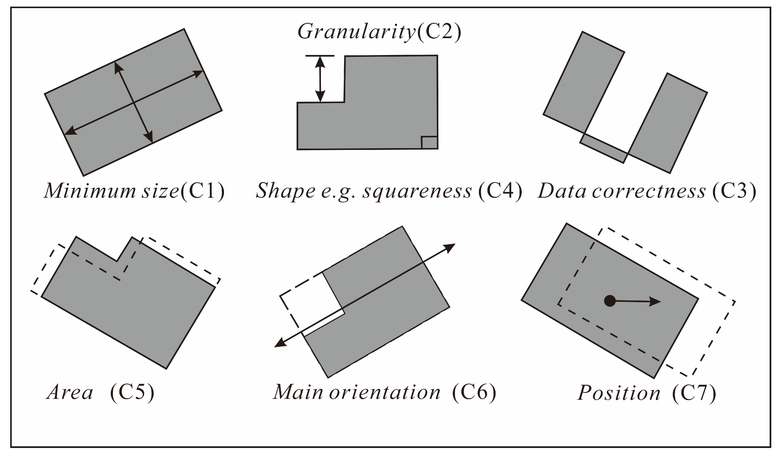
2.1. Building Simplification Constraints
- Granularity (C2): Building edges needs to be large enough to avoid visual confusion, e.g., 0.3 mm [25].
- Data correctness (C3): No data error is allowed, e.g., self-intersection [26].
- Shape (C4): The building shape needs to be maintained, e.g., orthogonal features [27].
- Size (C5): The building area needs to be maintained [25].
- Orientation (C6): The main orientation of the building needs to be maintained [28].
- Position (C7): The simplified building needs to be close to its original position [29].
2.2. Building Simplification Approaches
3. Methodology
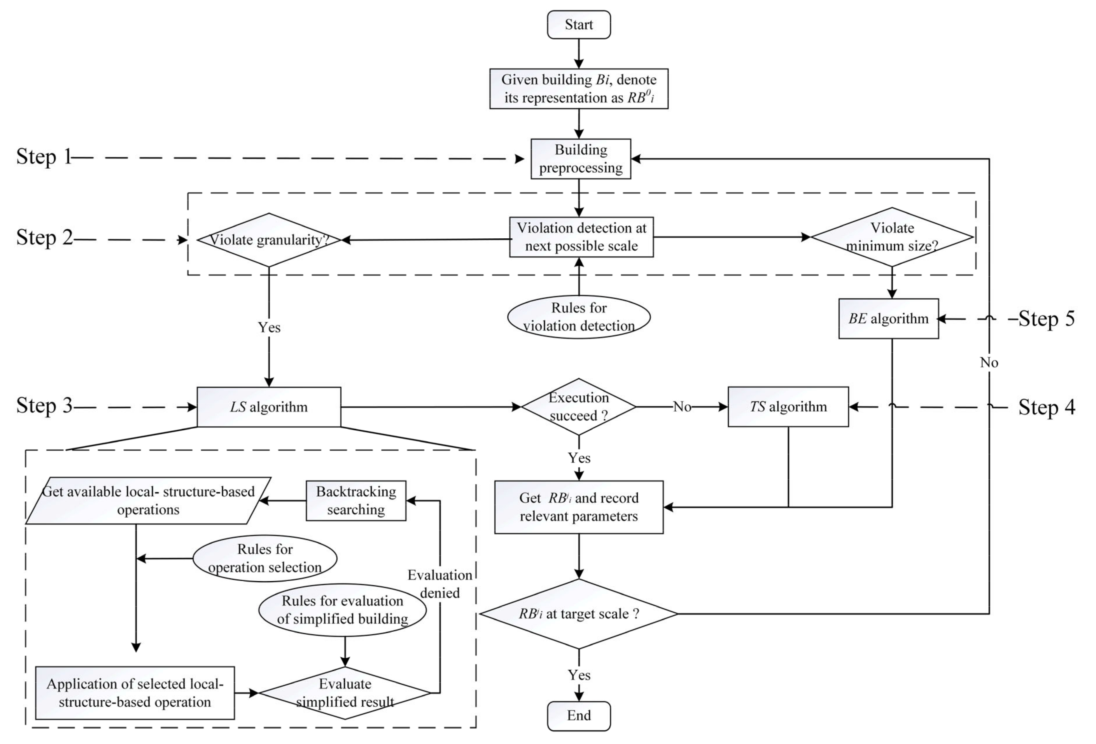
3.1. Framework
- Step 1.
- Perform preprocessing to remove potential abnormal nodes of buildings before applying any simplification operation (Section 3.2.)
- Step 2.
- Violation detection at the next possible scale. Violations are defined based on whether the legibility constraints are violated at the next possible scale (Section 3.3).
- Step 3.
- If RBji violates granularity constraints at the next possible scale, perform a local-structure-based simplification (LS) algorithm (Section 3.4). This algorithm classifies local structures and defines their based operations (Section 3.4.1). Rules considering preservation constraints supporting the application of local-structure-based operation at the current step are provided (Section 3.4.2). A backtracking searching strategy is also provided in case an invalid local-structure-based operation is applied. If a satisfactory result can be obtained with LS algorithm, return to Step 1; otherwise, proceed to Step 4. Whether the result is a satisfactory one is defined based on preservation constraints (Section 3.4.3).
- Step 4.
- If the LS algorithm cannot obtain a satisfactory result, use a template-based simplification (TS) algorithm; then return to Step 1 (Section 3.5).
- Step 5.
- If the minimum size constraint will be violated at the next possible scale, use a building enlargement (BE) algorithm (Section 3.5).
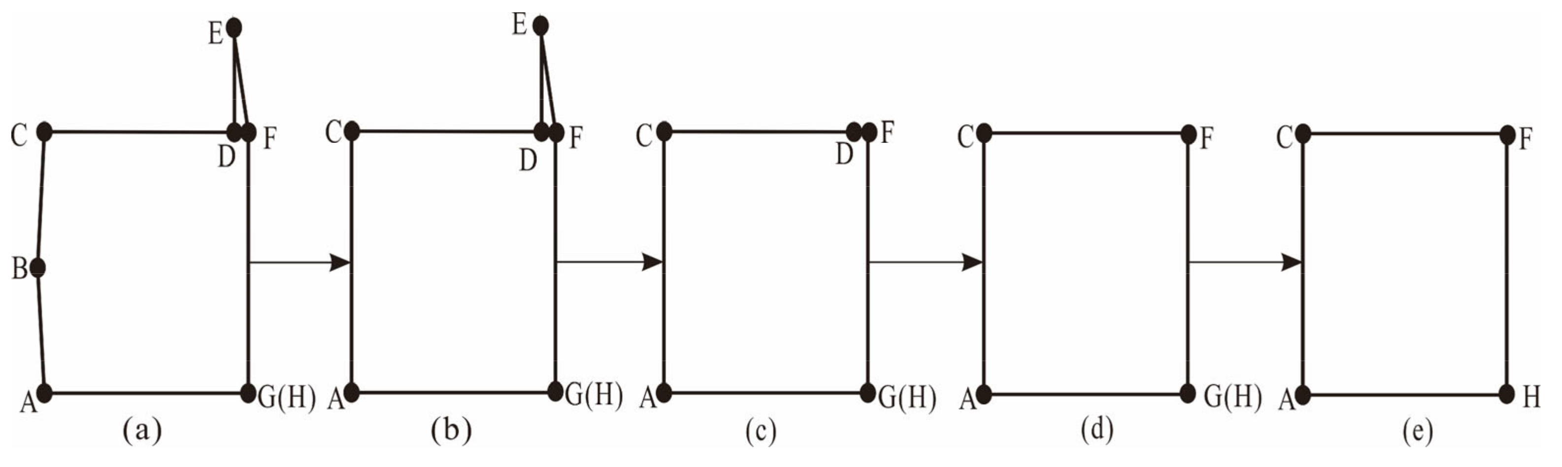
3.2. Step 1: Building Preprocessing
3.3. Step 2: Definitions of Legibility Constraint Violations
3.4. Step 3: Local-Structure-Based Simplification Algorithm
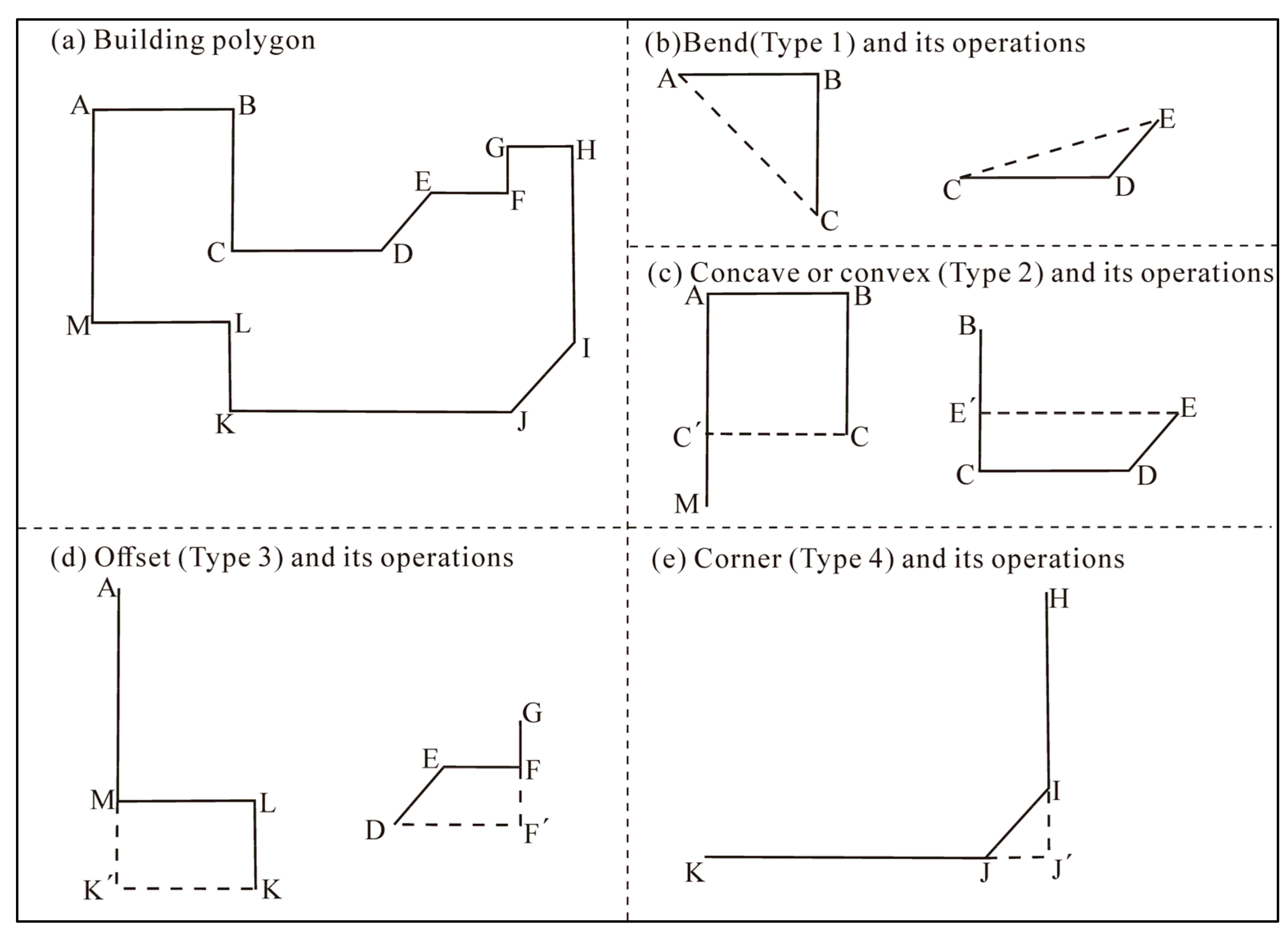
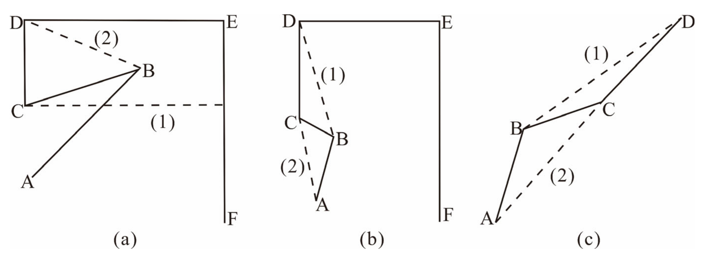
3.4.1. Local Structure Classification and Their Based Operations
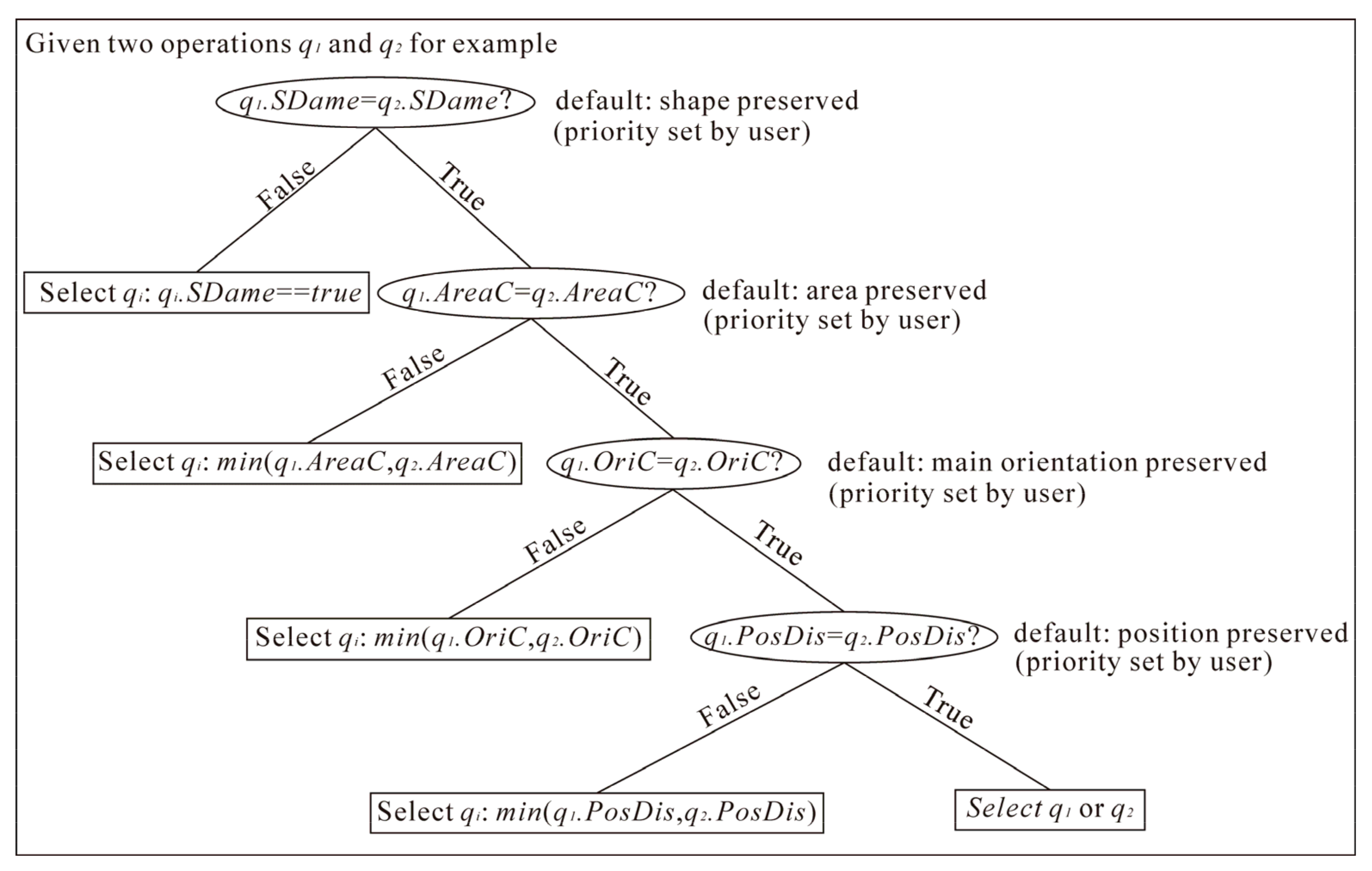
3.4.2. Selection of Applied Local-Structure-Based Operation
3.4.3. Evaluation and Backtracking Strategy
- Rule 1: If , then the result obtained by applying qn is evaluated as unsatisfactory.
- Rule 2: If , then the result obtained by applying qn is evaluated as unsatisfactory.
- Rule 3: If , then the result obtained by applying qn is evaluated as unsatisfactory.
- Rule 4: If the building obtained by applying the selected operation pn has fewer than four nodes, then it is evaluated as unsatisfactory.
| Backtracking strategy. |
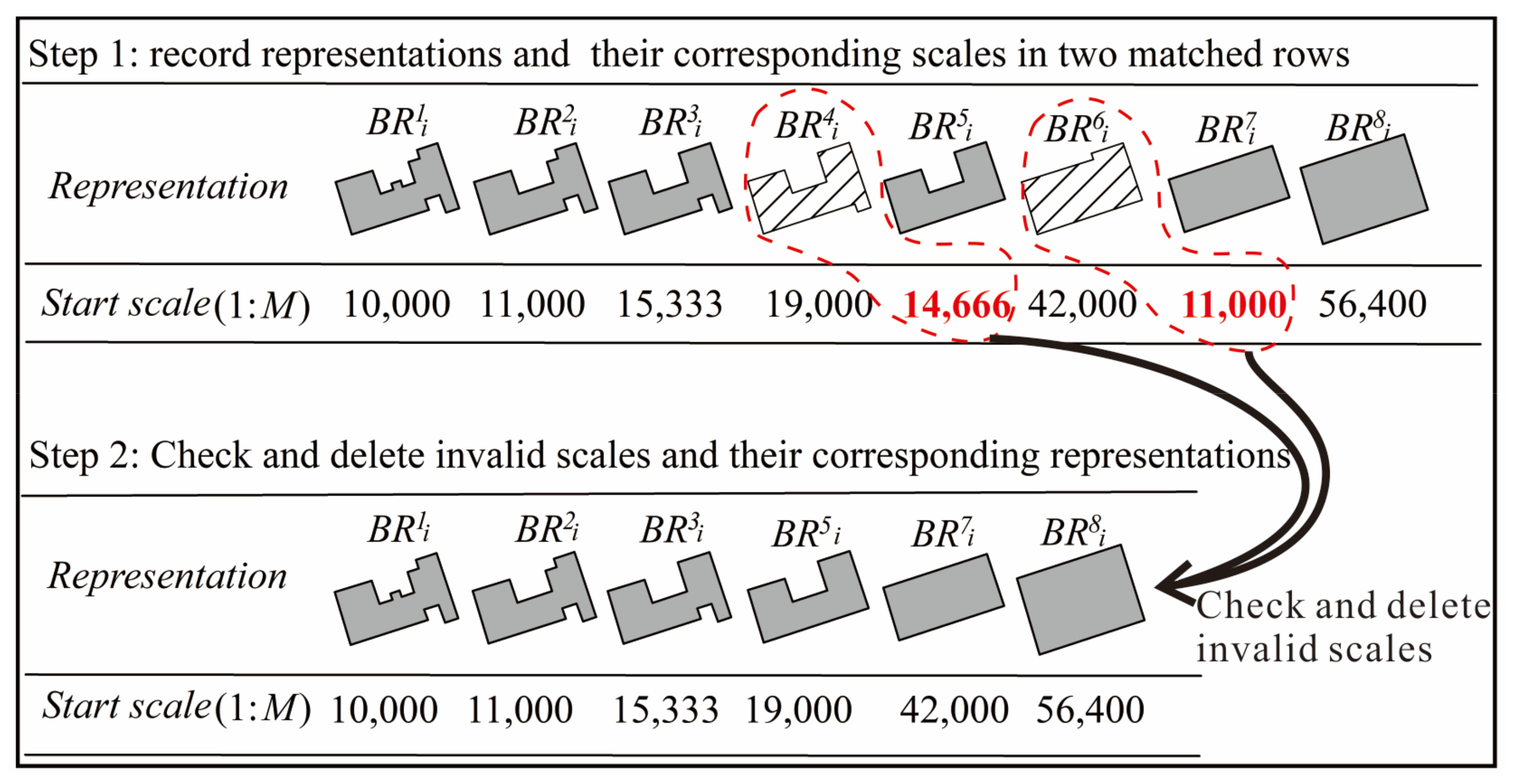
| Input: Obtained representations of Bi as , available operations for RBji in RBS as ; maximum searching step as MaxS Output: RBk Set searching step as p, and Get Qj: Obtain available operation set Qj based on RBji and start with When AND AND , Then Selection: Select an operation qmj in Qj based on the binary decision tree defined in Section 3.4.2 to obtain needs to be determined. If , remove qmj in Qj, Continue Else if , Then Evaluation: Determine whether RBki satisfies rules defined for simplified building: If evaluation accepted, Then return to RBki, End. Else if evaluation denied, remove qmj in Qj. When AND AND , Then , return to Get Qj Else Return null, End. |
3.5. Steps 4 and 5: Template-Based and Building Enlargement Simplification
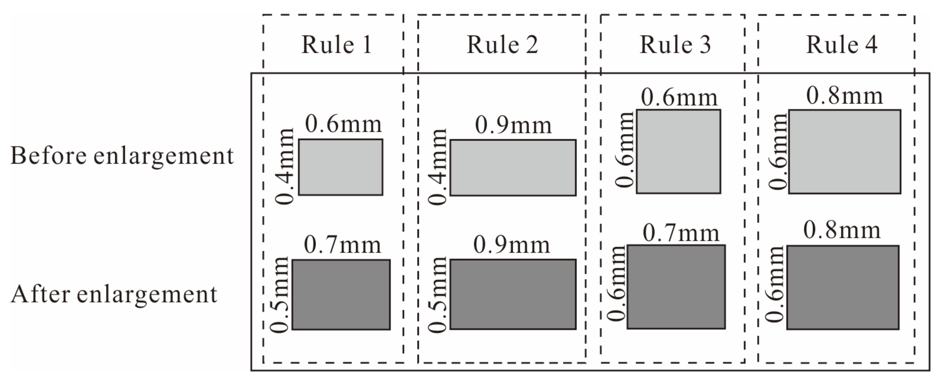
- Rule 1: If Bi violates STa at the next possible scale, it is enlarged by replacing it with a rectangle as STL × STW.
- Rule 2: If Bi violates STW at the next possible scale, it is enlarged by replacing it with a rectangle as LBi × STW.
- Rule 3: If Bi violates STL at the next possible scale, it is enlarged by replacing it with a rectangle as WBi × STL.
- Rule 4: If no violation of minimum size constraint is found at the next possible scale, no building enlargement will be performed.
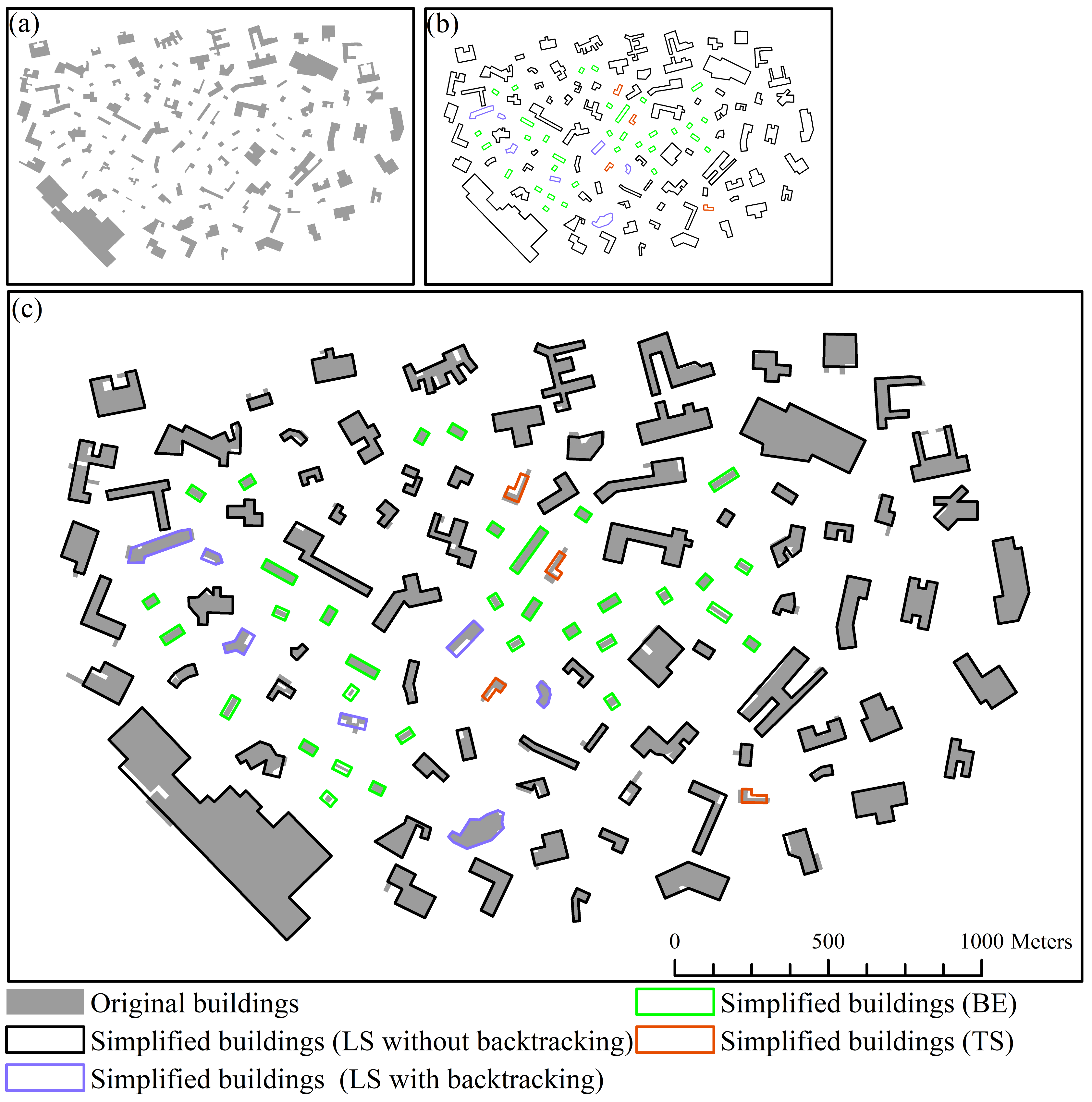
4. Experiment
5. Discussion
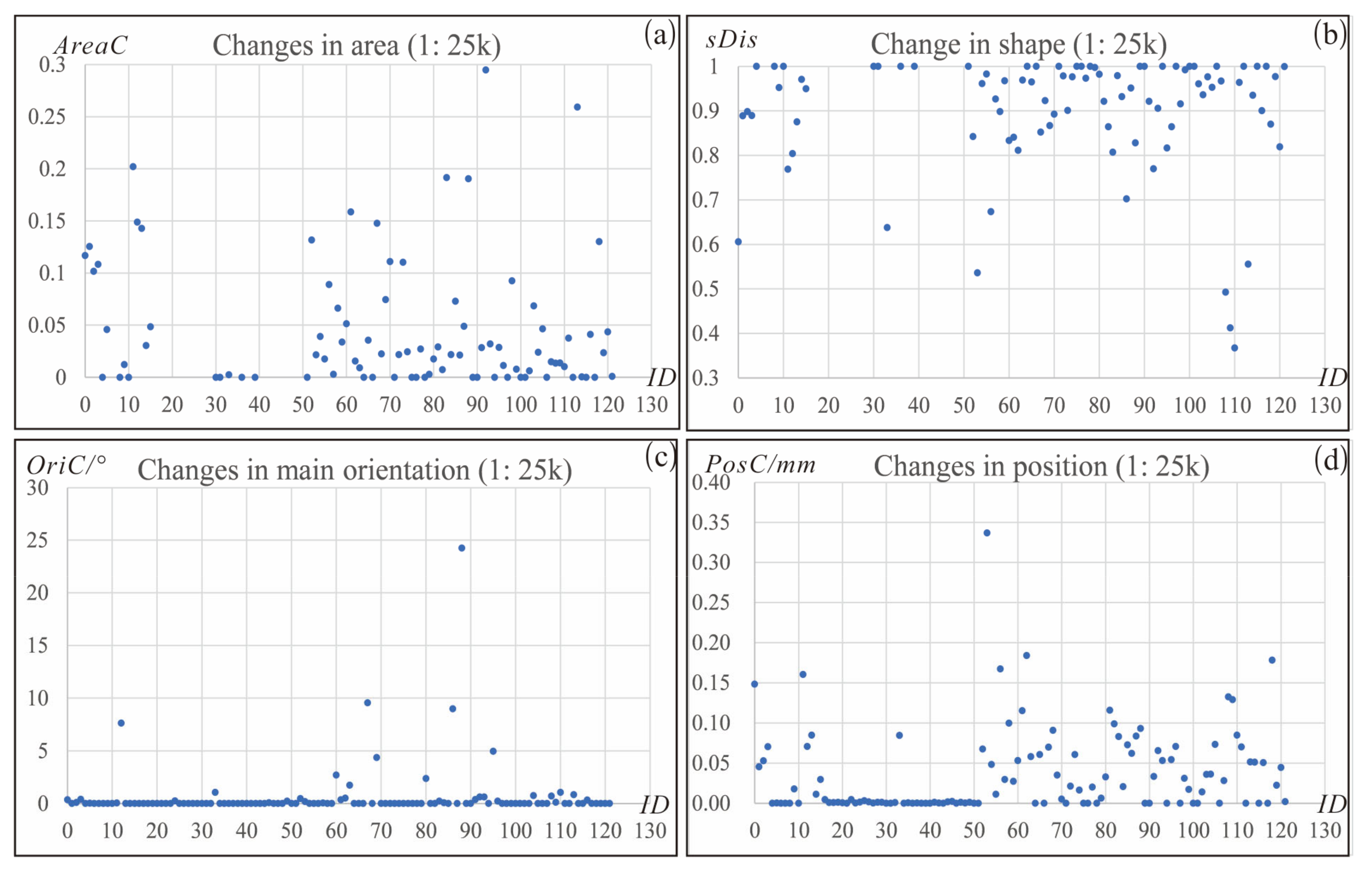
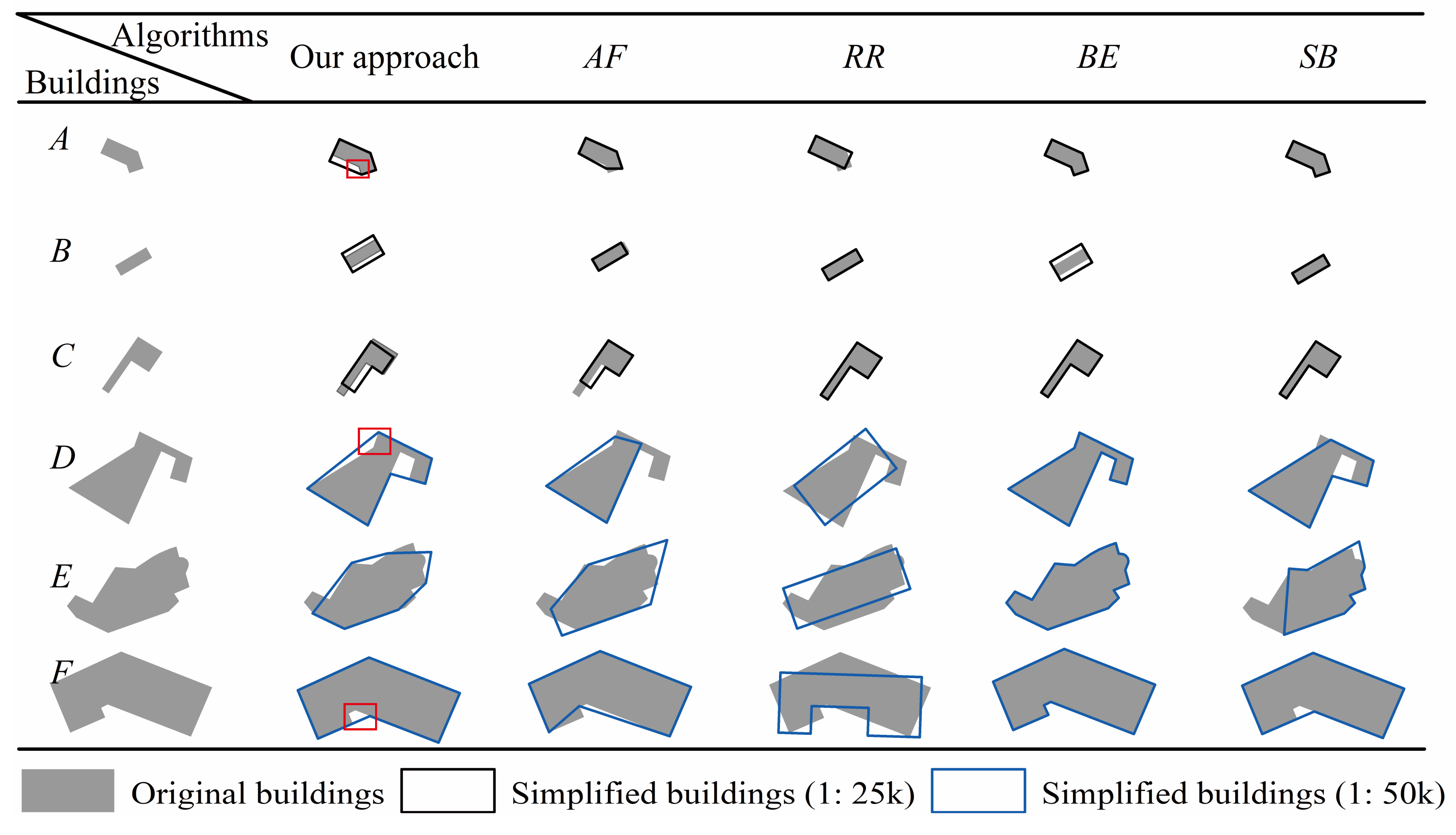
5.1. Comparisons
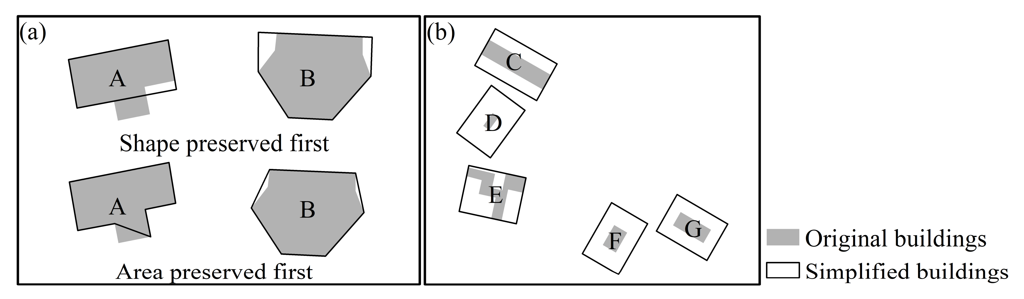
5.2. Possible Use for Continuous Scale Transformation of Buildings
5.3. Limitations
6. Conclusions
Author Contributions
Funding
Data Availability Statement
Acknowledgments
Conflicts of Interest
References
- Lee, D. New cartographic generalization tools. In Proceedings of the 19th International Cartographic Conference of the ICA, Ottawa, ON, Canada, 14–21 August 1999; pp. 1235–1242. [Google Scholar]
- Sester, M. Generalization based on least squares adjustment. Int. Arch. Photogramm. Remote Sens. 2000, XXXIII, 931–938. [Google Scholar]
- Ai, T.; Cheng, X.; Liu, P.; Yang, M. A shape analysis and template matching of building features by the Fourier transform method. Comput. Environ. Urban Syst. 2013, 41, 219–233. [Google Scholar] [CrossRef]
- Burghardt, D.; Schmid, S. Constraint-based evaluation of automated and manual generalized topographic maps. In Cartography in Central and Eastern Europe; Springer: Berlin, Heidelberg, 2009; pp. 147–162. [Google Scholar]
- Rainsford, D.; Mackaness, W. Template matching in support of generalization of rural buildings. In Advances in Spatial Data Handling, Proceedings of the 10th International Symposium on Spatial Data Handling, Ottawa, ON, Canada, 9–12 July; Richardson, D.E., Van O, P., Eds.; Springer: Berlin/Heidelberg, Germany, 2002; pp. 137–151. [Google Scholar]
- Yan, X.; Ai, T.; Zhang, X. Template matching and simplification method for building features based on shape cognition. Int. J. Geo Inf. 2017, 6, 250. [Google Scholar] [CrossRef] [Green Version]
- Wang, L.; Guo, Q.; Liu, Y.; Sun, Y.; Wei, Z. Contextual Building Selection Based on a Genetic Algorithm in Map Generalization. Int. J. Geo Inf. 2017, 6, 271. [Google Scholar] [CrossRef]
- Guo, Q. The method of graphic simplification of area feature boundary as right angle. Geomat. Inf. Sci. Wuhan Univ. 1999, 24, 255–258. [Google Scholar]
- Sester, M. Optimization approaches for generalization and data abstraction. Int. J. Geogr. Inf. Sci. 2005, 19, 871–897. [Google Scholar] [CrossRef]
- Chen, W.; Long, Y.; Shen, J.; Li, W. Structure recognition and progressive of then concaves of building polygon based on constrained D-Tin. Geomat. Inf. Sci. Wuhan Univ. 2011, 36, 584–587. [Google Scholar]
- Cheng, B.; Liu, Q.; Li, X.; Wang, Y. Building simplification using backpropagation neural networks: A combination of cartographers’ expertise and raster-based local perception. GISci. Remote Sens. 2013, 50, 527–542. [Google Scholar] [CrossRef]
- Buchin, K.; Meulemans, W.; Renssen, A.V.; Speckmann, B. Area-preserving simplification and schematization of polygonal subdivisions. ACM Trans. Spat. Algorithms Syst. 2016, 2, 1–36. [Google Scholar] [CrossRef]
- Oosterom, P.V.; Meijers, M. Vario-scale data structures supporting smooth zoom and progressive transfer of 2D and 3D data. Int. J. Geogr. Inf. Sci. 2014, 28, 455–478. [Google Scholar] [CrossRef] [Green Version]
- Huang, L.; Ai, T.; Oosterom, P.V.; Yan, X.; Yang, M. A matrix-based structure for vario-scale vector representation over a wide range of map scales: The case of river network data. ISPRS Int. J. Geo-Inf. 2017, 6, 218. [Google Scholar] [CrossRef] [Green Version]
- Peng, D.; Touya, G. Continuously generalizing buildings to built-up areas by aggregating and growing. In UrbanGIS’17: 3rd ACM SIGSPATIAL Workshop on Smart Cities and Urban Analytics, 7–10 November 2017, Redondo Beach, CA, USA; ACM: New York, NY, USA, 2017; 8p. [Google Scholar]
- Shen, Y.; Ai, T.; Li, C. A simplification of urban buildings to preserve geometric properties using superpixel segmentation. Int. J. Appl. Earth Observ. Geoinf. 2019, 79, 162–174. [Google Scholar] [CrossRef]
- Wang, Z.; Lee, D. Building simplification based on pattern recognition and shape analysis. In Proceedings of the 9th International Symposium on Spatial Data Handling, Beijing, China, 10–12 August 2000; pp. 58–72. [Google Scholar]
- Steiniger, S.; Taillandier, P.; Weibel, R. Utilising urban context recognition and machine learning to improve the generalization of buildings. Int. J. Geogr. Inf. Sci. 2010, 24, 253–282. [Google Scholar] [CrossRef]
- Ruas, A. Modèle de Généralisation de Données Géographiques à Base de Contraintes et d’autonomie. Ph.D. Thesis, Sciences de l’Information G´eographique, Marne La Vallee, France, 1999. [Google Scholar]
- Duchêne, C.; Christophe, S.; Ruas, A. Generalisation, symbol specification and map evaluation: Feedback from research done at COGIT laboratory, IGN France. Int. J. Digit. Earth 2011, 4 (Suppl. S1), 25–41. [Google Scholar] [CrossRef]
- Duchêne, C.; Ruas, A.; Christophe, C. The CartACom model: Transforming cartographic features into communicating agents for cartographic generalization. Cartogr. Geogr. Inf. Syst. 2012, 26, 1533–1562. [Google Scholar] [CrossRef]
- Maudet, A.; Touya, G.; Duchêne, C.; Picault, S. DIOGEN, a multi-level oriented model for cartographic generalization. Int. J. Cartogr. 2017, 3, 121–133. [Google Scholar] [CrossRef]
- Wang, L.; Guo, Q.; Wei, Z.; Liu, Y. Spatial conflict resolution in a multi-agent process by the use of a snake model. IEEE Access 2017, 5, 24249–24261. [Google Scholar] [CrossRef]
- Stoter, J.; Smaalen, J.; Bakker, N.; Hardy, P. Specifying Map Requirements for Automated Generalization of Topographic Data. Cartogr. J. 2009, 46, 214–227. [Google Scholar] [CrossRef]
- Regnauld, N. Contextual building typification in automated map generalization. Algorithmica 2001, 30, 312–333. [Google Scholar] [CrossRef]
- Xu, W.; Long, Y.; Zhou, T.; Chen, L. Simplification of building polygon based on adjacent four-point method. Acta Geod. Cartogr. Sin. 2013, 42, 929–936. [Google Scholar]
- Lokhat, I.; Touya, G. Enhancing building footprints with squaring operations. J. Spat. Inf. Sci. 2016, 13, 33–60. [Google Scholar] [CrossRef]
- Duchêne, C.; Bard, S.; Barillot, X. Quantitative and qualitative descr-iption of building orientation. In Proceedings of the 5th Workshop on Progress in Automated Map Generalization, Paris, France, 28–30 April 2003. [Google Scholar]
- Liu, Y.; Guo, Q.; Sun, Y.; Ma, X. A combined approach to cartographic displacement for buildings based on skeleton and improved elastic beam algorithm. PLoS ONE 2014, 9, e113953. [Google Scholar] [CrossRef] [PubMed]
- Zhang, X.; Stoter, J.; Ai, T.; Kraak, M.-J.; Molenaar, M. Automated evaluation of building alignments in generalized maps. Int. J. Geogr. Inf. Sci. 2013, 27, 1550–1571. [Google Scholar] [CrossRef]
- Bayer, T. Automated building simplification using a recursive approach. In Cartography in Central and Eastern Europe; Gartner, G., Ortag, F., Eds.; Springer: Berlin, Heidelberg, 2009; pp. 121–146. [Google Scholar]
- Damen, J.; van Kreveld, M.; Spaan, B. High quality building generalization by extending the morphological operators. In Proceedings of the 12th ICA Workshop on Generalization and Multiple Representation, Montpellier, France, 20–21 June 2008. [Google Scholar]
- Meijers, M. Building simplification using offset curves obtained from the straight skeleton. In Proceedings of the 19th ICA Workshop on Generalisation and Multiple Representation, Helsinki, Finland, 14 June 2016. [Google Scholar]
- Kada, M. Aggregation of 3D buildings using a hybrid data approach. Cartogr. Geogr. Inf. Syst. 2011, 38, 153–160. [Google Scholar] [CrossRef]
- Wei, Z.; He, J.; Wang, L.; Wang, Y.; Guo, Q. A collaborative displacement approach for spatial conflicts in urban building map generalization. IEEE Access 2018. [Google Scholar] [CrossRef]
- Fan, H.; Alexander, Z.; Wu, H. Detecting repetitive structures on building footprints for the purposes of 3D modeling and reconstruction. Int. J. Digit. Earth 2017, 10, 785–797. [Google Scholar] [CrossRef]
- Shen, Y.; Ai, T.; He, Y. A new approach to line simplification based on image processing: A case study of water area boundaries. ISPRS Int. J. Geo-Inf. 2018, 7, 41. [Google Scholar] [CrossRef] [Green Version]
- Taillandier, P.; Duchêne, C.; Drogoul, A. Automatic revision of rules used to guide the generalization process in systems based on a trial and error strategy. Int. J. Geogr. Inf. Sci. 2011, 25, 1971–1999. [Google Scholar] [CrossRef]
- Yang, M.; Yuan, T.; Yan, X.; Ai, T.; Jiang, C. A hybrid approach to building simplification with an evaluator from a backpropagation neural network. Int. J. Geogr. Inf. Sci. 2021. [Google Scholar] [CrossRef]
- National Administration of Surveying, Mapping and Geoinformation of China. Compilation Specification for National Fundamental Scale Maps-Part1: Complilation Specifications for 1:25,000, 1:50,000 & 1:100,000 Topographic Maps; China Zhijian Publishing House: Beijing, China, 2008.
- Ordnance Survey. OS OPEN MAP-LOCAL: Product Guide and Technical Specification. 2016. Available online: https://www.ordnancesurvey.co.uk/documents/os-open-map-local-product-guide.pdf (accessed on 21 October 2020).


| Description | Constraint Violation |
|---|---|
| Minimum size (violates STa) | |
| Minimum size (violates STL) | |
| Minimum size (violates STW) | |
| Granularity (violates GTL) |
| Field | Type | Description |
|---|---|---|
| ID | Int | Unique building identification code. |
| SType | Int | Denotes type of local structure: 1 = bend, 2 = convex or concave, 3 = offset, 4 = corner. |
| IsInt | Bool | Denotes whether self-intersection is generated after applying qn: true or false. |
| SDame | Bool | Denotes whether orthogonal features are damaged after applying qn: true or false. |
| AreaC | Double | Denotes area change rate by comparing to original after applying qn, as , in which AreaA is the area of original one, AreaS is the area of the obtained building after applying qn. |
| OriC | Double | Denotes main orientation change compared to original after applying qn, as , in which OriC is the MBR orientation of the original one, OriS is the MBR orientation of the obtained building after applying qn. |
| PosC | Double | Denotes displaced distance by comparing to original after applying qn. |
| Scale | Number of Simplified Buildings | |||
|---|---|---|---|---|
| LS without Backtracking | LS without Backtracking | TS | BE | |
| 1: 25k | 78 | 7 | 4 | 33 |
| Scale | Measures | Our Approach | AF | RR | BE | SB |
|---|---|---|---|---|---|---|
| 1:25k | BNS | 0 | 36 | 42 | 0 | 33 |
| BNG | 0 | 1 | 7 | 65 | 47 | |
| aAreaC | 0.809 | 0.009 | 0.091 | 0.775 | 0.013 | |
| aOriC/° | 0.627 | 1.000 | 0.742 | 0.002 | 1.189 | |
| aPosC/mm | 0.040 | 0.020 | 0.042 | 0.000 | 0.012 | |
| asDis | 0.819 | 0.926 | 0.855 | 0.893 | 0.972 |
| Representation | BR1i | BR2i | BR3i | BR4i | BR5i | BR6i | BR7i | BR8i |
|---|---|---|---|---|---|---|---|---|
| AreaB (m2) | 1370 | 1357 | 1386 | 1421 | 1390 | 1626 | 1601 | 2300 |
| LB (m) | 56.8 | 56.8 | 56.8 | 56.8 | 56.8 | 56.8 | 56.8 | 56.8 |
| WB (m) | 35.3 | 35.3 | 35.3 | 35.3 | 31.0 | 3.3 | 28.2 | 40.5 |
| MLe (m) | 3.3 | 4.6 | 5.7 | 4.4 | 12.6 | 3.3 | 28.2 | 40.5 |
| Violation | GTL | GTL | GTL | GTL | GTL | GTL | GTL | STW |
| Start scale (1:M) | 10,000 | 11,000 | 15,333 | 19,000 | 14,666 | 42,000 | 11,000 | 56,400 |
| Validation | Valid | Valid | Valid | Valid | Invalid | Valid | Invalid | Valid |
Publisher’s Note: MDPI stays neutral with regard to jurisdictional claims in published maps and institutional affiliations. |
© 2021 by the authors. Licensee MDPI, Basel, Switzerland. This article is an open access article distributed under the terms and conditions of the Creative Commons Attribution (CC BY) license (https://creativecommons.org/licenses/by/4.0/).
Share and Cite
Wei, Z.; Liu, Y.; Cheng, L.; Ding, S. A Progressive and Combined Building Simplification Approach with Local Structure Classification and Backtracking Strategy. ISPRS Int. J. Geo-Inf. 2021, 10, 302. https://doi.org/10.3390/ijgi10050302
Wei Z, Liu Y, Cheng L, Ding S. A Progressive and Combined Building Simplification Approach with Local Structure Classification and Backtracking Strategy. ISPRS International Journal of Geo-Information. 2021; 10(5):302. https://doi.org/10.3390/ijgi10050302
Chicago/Turabian StyleWei, Zhiwei, Yang Liu, Lu Cheng, and Su Ding. 2021. "A Progressive and Combined Building Simplification Approach with Local Structure Classification and Backtracking Strategy" ISPRS International Journal of Geo-Information 10, no. 5: 302. https://doi.org/10.3390/ijgi10050302