
Spatial and Temporal Characteristic Analysis of Imbalance Usage in the Hangzhou Public Bicycle System


1
School of Spatial Planning and Design, Zhejiang University City College, Hangzhou 310058, China
2
School of Earth Sciences, Zhejiang University, Hangzhou 310027, China
3
School of Information Systems and Technology, Claremont Graduate University, Claremont, CA 91711, USA
*
Author to whom correspondence should be addressed.
ISPRS Int. J. Geo-Inf. 2021, 10(10), 637; https://doi.org/10.3390/ijgi10100637
Submission received: 5 August 2021
/
Revised: 10 September 2021
/
Accepted: 16 September 2021
/
Published: 24 September 2021
(This article belongs to the Special Issue Geovisualization and Social Media)
Abstract
:Calculating the availability of bicycles and racks is a traditional method for detecting imbalance usage in a public bicycle system (PBS). However, for bike-sharing systems in Asian countries, which have compact layouts and larger system scales, an alternative docking station may be found within walking distance. In this paper, we proposed a synthetic and spatial-explicit approach to discover the imbalance usage by using the Hangzhou public bicycle system as an example. A spatial filter was used to remove the false-alarm docking stations and to obtain true imbalance areas of interest (AOI), where the system operation department installs more stations or increases the capacity of existing stations. In addition, sub-nearest neighbor analysis was adopted to determine the average distance between stations, resulting in an average station spacing of 190 m rather than 15.5 m, which can reflect the nonbiased service level of Hangzhou’s public bicycle systems. Our study shows that neighboring stations are taken into account when analyzing PBSs that use a staggered or face-to-face layout, and our method can reduce the number of problematic stations that need to be reallocated by about 92.81%.
1. Introduction
A public bicycle system (PBS) is an essential component of urban transportation systems. It can reduce car use, alleviate traffic congestion [1], increase transportation connectivity [2] and supplement other means of transportation [3,4,5]. Additionally, a public bicycle system can help save travel time during the rush hour [6], help people to stay fit [2,7,8], and reduce vehicle emissions [2]. Thus, governments are experimenting with various methods to support the development of public bicycles. There are globally already more than 2000 public bicycle systems in operation [9,10]. Among them, Chinese public bicycle systems sprouted from 2008, and its total number of public bicycles in 2014 surpassed the total number of those of all other countries [11]. As a pioneering public bicycle system in China, the Hangzhou public bicycle system is developed and a popular travel choice for the citizens.
With the application of RFID technology and information management systems [12], usage records are available. Geographers, urban planners, and transportation administrators extensively studied and debated various aspects of trip-demand analysis for public bicycle systems [13,14,15,16]. Corcoran et al. [17] classified these studies on the basis of their source data into two categories: docking-station [18,19,20,21,22] and journey [13,23,24,25] data analysis. Docking-station data are sampled at fixed intervals and provide real-time capacity, whereas journey data provide the origin and destination pair stations of each user. In comparison to journey data, docking-station data are much more accessible through the open application programming interface (API) provided by many PBS administrators for third-party developers to create add-in functions.
The literature on docking-station data analysis reveals the spatial–temporal dependency and driven factor of travel demand [20,23,26]. For example, the most significant driven factor varies between weekends and weekdays [18]. On weekdays, rental peaks occur during rush hour in the morning and late afternoon, indicating the purpose of commuting. On weekends, the morning peak usually disappears or is delayed by around two hours. Other factors that may affect travel demand include terrain [20], land use [9,22], weather [19,22] and major events [19]. Furthermore, the spatial–temporal characteristics of travel demand might disclose land use in the surrounding area [18]. Docking stations near businesses and commercial areas operate on the mode of returning in the morning and renting in the evening [20]; those near famous tourist attractions are more frequently visited throughout the day, whereas those near residential areas are more commonly used in the morning than in the evening [22].
One hot issue among all travel-demand analysis is imbalance utilization, which has a tight relationship with new site selection, rebalancing activities, user satisfaction, and the improvements in service quality [4,27,28]. An imbalance occurs when the docking station’s service capacity is insufficient to fulfill customer demand due to traffic flow asymmetry [14,23]. Studies proposed different methods to detect imbalance usage. Borgnat et al. [29] identified imbalanced docking stations by examining whether the absolute value of the difference between incoming and outgoing trips is larger than three times the standard deviation. Fricker and Gast [30] used the term “problematic station” to describe the station’s imbalance demand, which they further classified into two types: not enough bicycles and not enough racks. O’mahony and Shmoys [31], and Ciancia et al. [32] used normalized available bicycles (NAB) to identify imbalance stations and develop bike repositioning strategies. Wang et al. [19] first applied geographic analysis to this problem, categorized problematic stations on the basis of NAB, quantified the degree of imbalance, and displayed it in line chart with time as abscissa. Their research revealed that the distribution of the imbalanced period corresponds to the peak period. Maleki Vishkaei et al. [27] produced NAB as a decision variable and constructed its decision model for PBSs. They tried to find a proactive policy balancing the whole system.
In Asian countries’ public bicycle systems, to serve more people and reach a larger service area, PBSs tend to have a more densely distributed spatial configuration. This means that neighbor stations are close and can provide alternative services to each other. When a citizen finds that a station is full or empty, there may be another station just a few hundred meters away. This situation is very common, especially in urban central areas where travel demand frequently surges and decreases. Thus, an imbalance station may be temporal or “feak”, simply counting the number of available bicycles does not indicate the actual imbalance. The identification process should include spatial neighbors, surrounding stations, into the analysis to determine the unbalanced area where the system operator should intervene.
In this research, we propose a docking-station data-driven approach to detecting real imbalanced areas of the Hangzhou public bicycle system. Unlike other approaches, we identified problematic stations by using an extra spatial filtering procedure and aggregating them into areas of interest (AOI). The main contribution of this study is the synthetic and spatial explicit approach that broadens the definition of problematic station to imbalance AOI. It addresses the fact that imbalance usage detection should not be limited to imbalance docking stations, but should be applied to an entire area of clustered docking stations where regular services cannot be delivered. The second contribution is the use of sub-nearest neighbor analysis to measure station spacing. Our analytical results show that it can provide a more precise definition of the station spacing metric for staggered or face-to-face layout PBSs.
The rest of the content is organized as follows. Section 2 introduces the Hangzhou public bicycle system and data sources. Section 3 focuses on the methods for exploring the overall layout and detecting the imbalance region. In Section 4, we present the results of analysis and detection, and make appropriate interpretations on the basis of the actual situation in Hangzhou. We discuss the reliability of results and the shortcomings of the methods in Section 5. Lastly, in Section 6, we summarize the research works and discuss the future directions of this paper.
2. Background
2.1. Hangzhou Public Bicycle System
Driven by the sustainable development of the city, in 1 May 2008, Hangzhou took the lead in running the public bicycle system as a new form of urban transportation in the entire country [33]. The Hangzhou public bicycle system is classified as a third-generation bike sharing program in terms of utilization and docking-station configurations [34]. It was primarily established for solving the problem of “the last kilometer to end a transit trip” [35], and could provide service for tourists to visit scenic spots such as the famous West Lake [36].
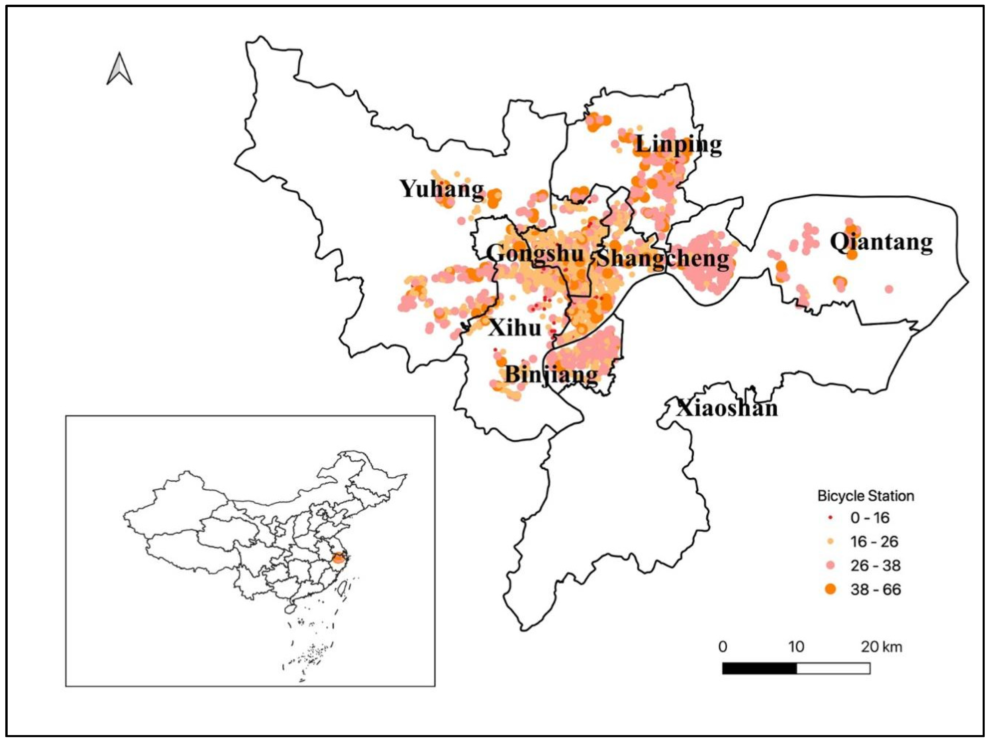
By the end of December 2018, there were 4198 docking stations and 1,017,000 public bicycles, according to data from the Hangzhou public cycling system’s official website. The maximal daily rental amount was 473,000. The overall rental amount topped 925 million, and the free usage rate exceeded 96% [37]. The geographical location of the study area and the distribution of public bicycle system are shown in Figure 1.
2.2. Data
Docking-station data of the Hangzhou public bicycle system were acquired by a Python script that interacted with the capacity inquiry API. The API is provided by the system operator and official website. It provides real-time site stock information, including docking stations’ identification code, address, number of available docking stations, and number of available bicycles. We chose a sampling interval of 10 min from 7:00 a.m. to 22:00 p.m., and at other times, we used a sampling period of 20 min. Our study period began on 7 June 2019 and ended on 14 June 2019, including the Dragon Boat Festival (7–9 June) and five weekdays (10–14 June).
3. Method
3.1. Imbalance Usage Detection
The docking station has the two primary functions: rental and return. An important characteristic statistic for measuring its functionality is the normalized available bicycles or the load factor [20], which is commonly used to represent the availability of a bicycle station in a PBS in many studies [7,20,31,38]. It is the proportion of available bicycles in each docking station, as shown in Equation (1). The numerator is the number of bicycles parked in the station and available to users while they are not being used on the road. The greater the NAB is, the more bicycles are available in the docking station.
where denotes normalized available bicycles, represents the number of available bicycles, represents the number of docking points, and represents the number of available racks at the same time.
Imbalance usage can be depicted as two specific cases. The first case occurs as the NAB approaches 0, indicating that there are nearly no available bicycles in the docking station, and rental demand cannot be met. The other case is when the NAB approaches 1, implying that the bicycle racks in a docking station would run out, making it difficult to return. According to the definition, we define judgment rules as the Equation (2) to select stations where there may be imbalance demand. The former rule applies to the first case (Type A), while the latter applies to the second case (Type B).
where and are thresholds for judging whether conflicts occur.
3.2. Area-of-Interest Delineation
We extended the definition of problematic stations to include imbalance AOIs, where the same type of demand conflict (type A or B) co-occurs at the docking station and its surrounding docking stations. Residents are unable to use the PBS when the imbalance AOIs arise because there is no rental or return station within walking distance.
A three-step process was designed to detect these AOIs.
- ①
- Status calculation. The NAB of each station is calculated using Equation (1). Usage status is ascertained by the imbalance usage detection method shown as Equation (2). Then, at particular periods, stations in demand conflict are sifted out.
- ②
- Spatial filtering. Stations in the imbalance usage list from Step 2 are further validated by using a spatial filter. For each imbalance station, we find alternate workable stations that are not in conflict within neighbor scope. The neighboring scope is typically determined by the maximal walking distance. If no neighboring docking station is available, which means that all nearby stations are under the imbalance usage, we give the target station real imbalance status and add it to the list of imbalance stations as the input for AOI delineation. If one or more neighbors are available and can assist in the imbalance status, the target station is a fake imbalance station and is removed from the list of imbalance stations.
- ③
- AOI delineation. The final step is to aggregate all real imbalance stations and to generate demand conflict AOI. First, all stations are clustered into different groups, which requires that the distance between any stations that belongs to two different groups must be greater than walking distance, or these points are merged to form a new group. Then, AOIs are generated by concave hull algorithm and forms a minimum area containing a set of clustered stations. The concave hull can well describe the area occupied by the given set of points.
Figure 2 illustrates an example of an AOI detection and delineation workflow. The diamond points represent bicycle stations within the area in Figure 2a. After status calculation, there are 19 stations under imbalance usage, drawn as orange diamond points. Then, we execute spatial filtering operation one by one. When the red diamond point is chosen in Figure 2b, the stations within walking distance are all selected, and it is confirmed whether they are alternative stations. However, none is available now. Thus, the red diamond remains in the imbalance station lists.
After the spatial filtering operation, the stations under imbalance usage are fewer than the initial situation. There are only 10 stations left in Figure 2c. Since these stations are within walking distance, they aggregate into one demand conflict AOI in Figure 2d. The resulting AOI is at the top of the rebalancing schedule.
4. Results and Analysis
4.1. Temporal Characteristic of Imbalance Usage
4.1.1. NAB Results between Holidays and Weekdays
The number of available bicycles in a docking station might influence the usage frequency of public bicycles, and so indirectly affects convenience for public transit. A docking station’s ability to deliver public-bike-sharing services at different locations and times is not the same. In this section, we present the analytical results based on NAB to explore the temporal characteristics of public bicycle usage. The response API for the rent record of each station of 14 June at 08:00, 08:10, and 08:20 was −1; we used average NAB values to replace the outliers.
The average daily NAB during the study period is rendered and shown in Figure 3. To ensure the legibility of the diagram, high NAB values are expressed in red, and low NAB values in blue. The lower the NAB is, the more public bicycles are used. NAB clearly declined in a fluctuation way during the day, and gradually increased to its peak level at night.
The disparities in NAB results between holidays and weekdays are quite apparent. On holidays, the NAB showed one evident cold zone and one modest cold zone, whereas on weekdays, the NAB showed two narrow cold zones and a single peak in the afternoon. Furthermore, the morning peak on holidays is substantially later than that on weekdays. In terms of timing, the peak usage period on holidays is about 9:30 a.m. The morning peak lasts nearly two hours and then becomes more decentralized throughout the afternoon. On weekdays, the morning rush begins at around 8:20 a.m., and the afternoon rush begins at around 17:50 p.m.
The pattern represents the various roles that the Hangzhou public bicycle system plays in the daily lives of the city’s citizens. The morning rush hour on weekdays indicates a primary purpose of commuting, while afternoon or evening rush hours may vary depending on local social conventions and working hours. This phenomenon occurred with other PBSs as well. For example, the second peak of the Vienna public bicycle system occurs in the late afternoon hours, when commuting and leisure activities overlap [23]. In Barcelona, there is a usage peak at 14:00 p.m., when users leave their classes to go for lunch [18]. For the Hangzhou PBS, the afternoon rush is more likely to be caused by a combination of commuting, shopping, sightseeing, or other leisure activities. Furthermore, the lack of a clear usage peak during weekday noon indicates that neither office workers nor students have a habit of going out for lunch by bicycle.
On holidays, citizens often hold parties, group dinners, and outdoor activities. Hangzhou, as a typical tourist city, attracts numerous tourists, some of which may prefer to commute by public bicycle. The primary purpose of using public bicycles turns into entertainment. As a result, the NAB on weekdays is significantly smaller than that on holidays, implying that holiday usage was significantly lower than that on weekdays. Zhou [15] found that the intensity of public bicycle usage is lower on holidays than it is on weekends. Relevant international studies likewise reached the same conclusion: peak usage times are higher on weekdays [18,20,23].
An unusual phenomenon, shown in Figure 3, is that NAB on 13 June was significantly lower than the NAB of other weekdays. Rainy weather may affect the public bicycle usage of the day.
4.1.2. Imbalance Usage Detection Results
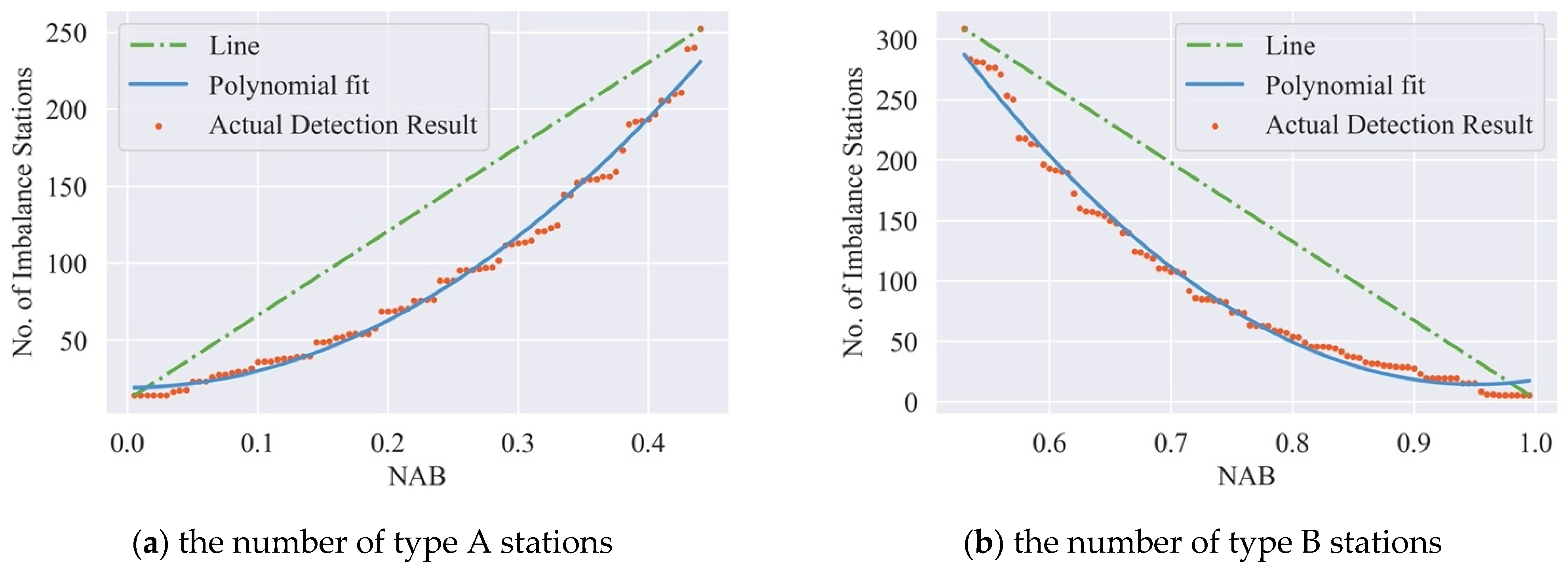
The imbalance usage detection method described in Equation (2) contains two parameters that can directly affect the results. Relevant studies typically select an approximate value on the basis of prior experiences, such as and . In our study, we performed sensitivity analysis to determine the upper and lower thresholds of NAB.
For conflict type A, conflict docking stations at 8:20 a.m. were detected by Equation (2) and spatially filtered. For conflict type B, the same detection was performed for docking stations at 24:00 p.m. Figure 4a,b show the detection result or types A and B, respectively. Red point was used to represent the actual detection results, which change nonlinearly with NAB. The polynomial fitting method was used to simulate the change of red scatter points, and the fitting curve was represented by a blue solid line. The green line of discontinuity was drawn to connect the start and the end of the red dot. The R2 of the Type A fitting curve was 0.9913, and the R2 of the Type B fitting curve was 0.9901, indicating that the fitting result was very close to the reality. Compared to linear curves with uniform change, fitting curves show a distinctive result at and separately.
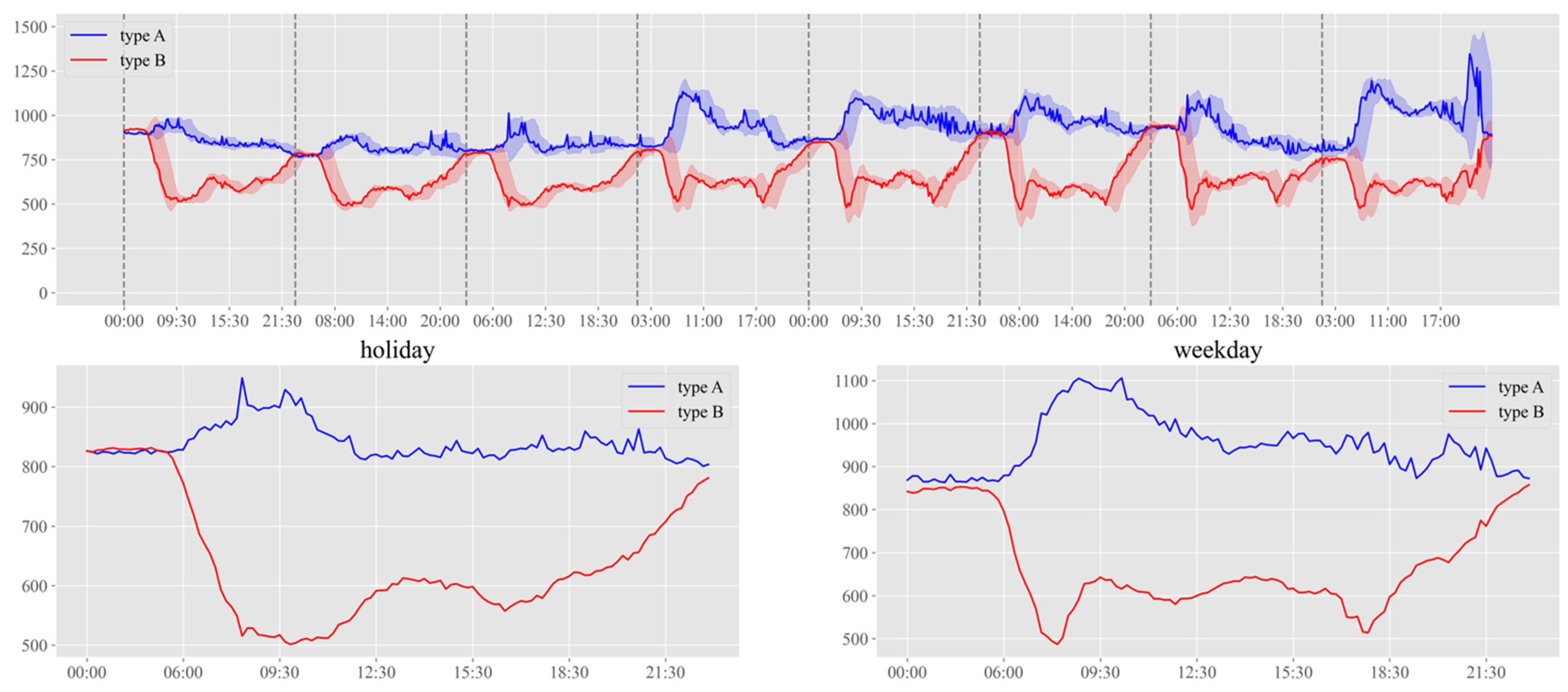
Thus, we used and in the imbalance-usage detection process to find problematic stations, and results are shown in Figure 5. The blue line (Type A) represents the number of docking stations with NABs less than 0.25, while the red line (Type B) represents the ones with a NABs greater than 0.74.
The 7–9 June are holidays during which the shape of the curves is repeated throughout the day. Another curve shape occurs and repeats on weekdays in 10–14 June. The two patterns are depicted in Figure 5. It is clear that the two types of demand conflict are mutually exclusive in time to some extent. While the rental imbalance usage (Type A) occurs, there is a substantial likelihood of finding less return imbalance usage (Type B) and vice versa. In general, the rental conflict (Type A) often occurs between 8:00 a.m. and 10:00 a.m., while the return conflict (Type B) often occurs between 22:00 p.m. and 06:00 a.m. the next morning, since this time is the night dispatching hour in the system operation.
There are some inconsistencies between weekdays and holidays. On weekdays, rental demand conflict occurs at 8:50 a.m., and docking stations with rental conflicts account for about 32% of the overall system. Return conflict typically occurs at 9:30 a.m., 14:30 p.m., and at 17:00 p.m., with docking stations accounting for about 16% of the total. On holidays, the rate of docking stations with rental demand conflict peaks from 9:00 a.m. to 11:00 a.m. and remains at around 18%, while the number of return conflict docking stations peaks from 14:00 p.m. to 16:30 p.m. Both types of demand conflicts exhibit a consistent and temporal clustering pattern. On this basis, whereas two conflict types are generally mutually exclusive, there are variances between holidays and weekdays. Furthermore, return conflict occurs at 24:00 p.m. on both weekdays and weekends, which may be caused by redistribution by bus company workers.
4.2. Spatial–Temporal Characteristics of Imbalance AOIs
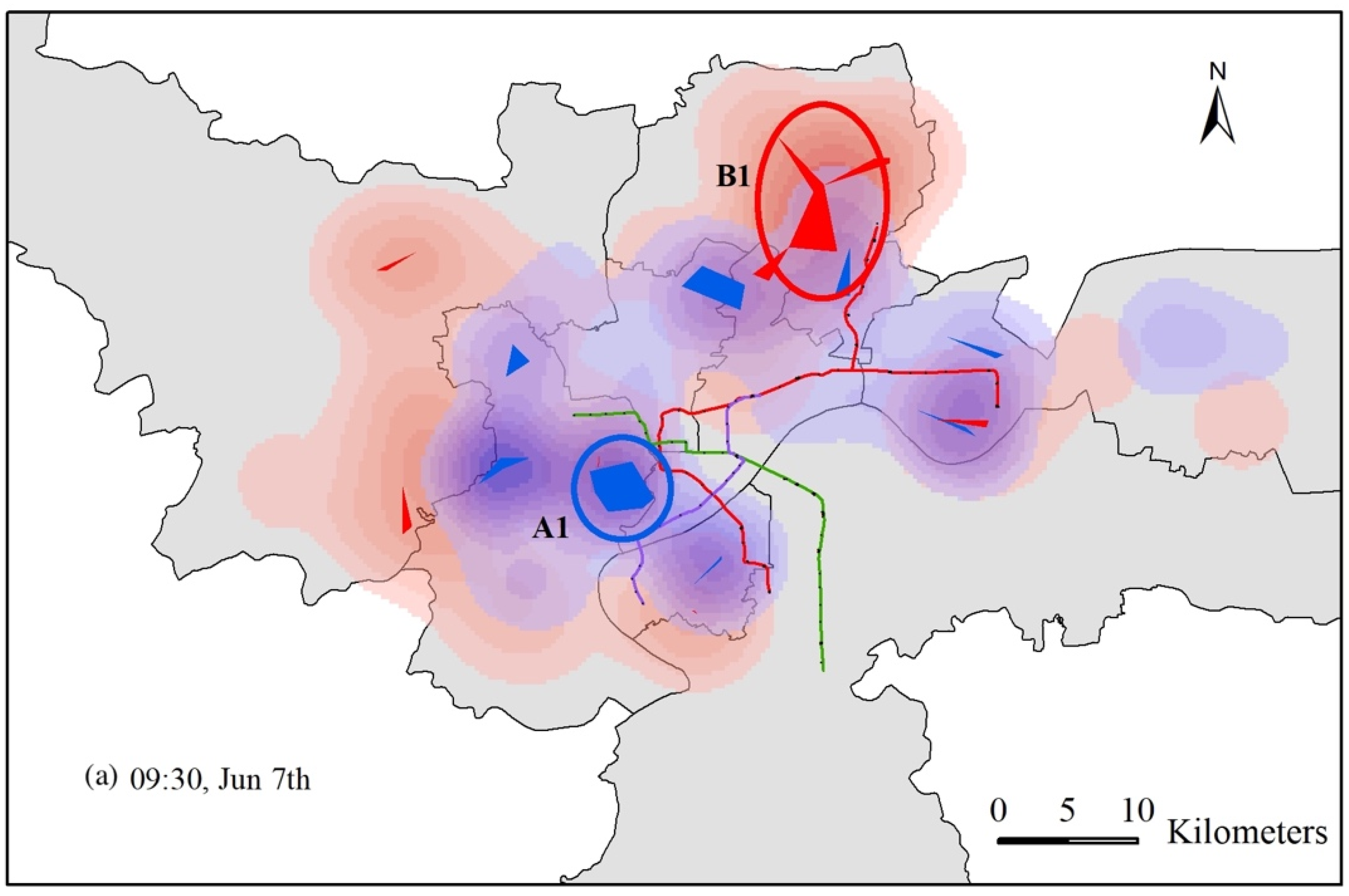
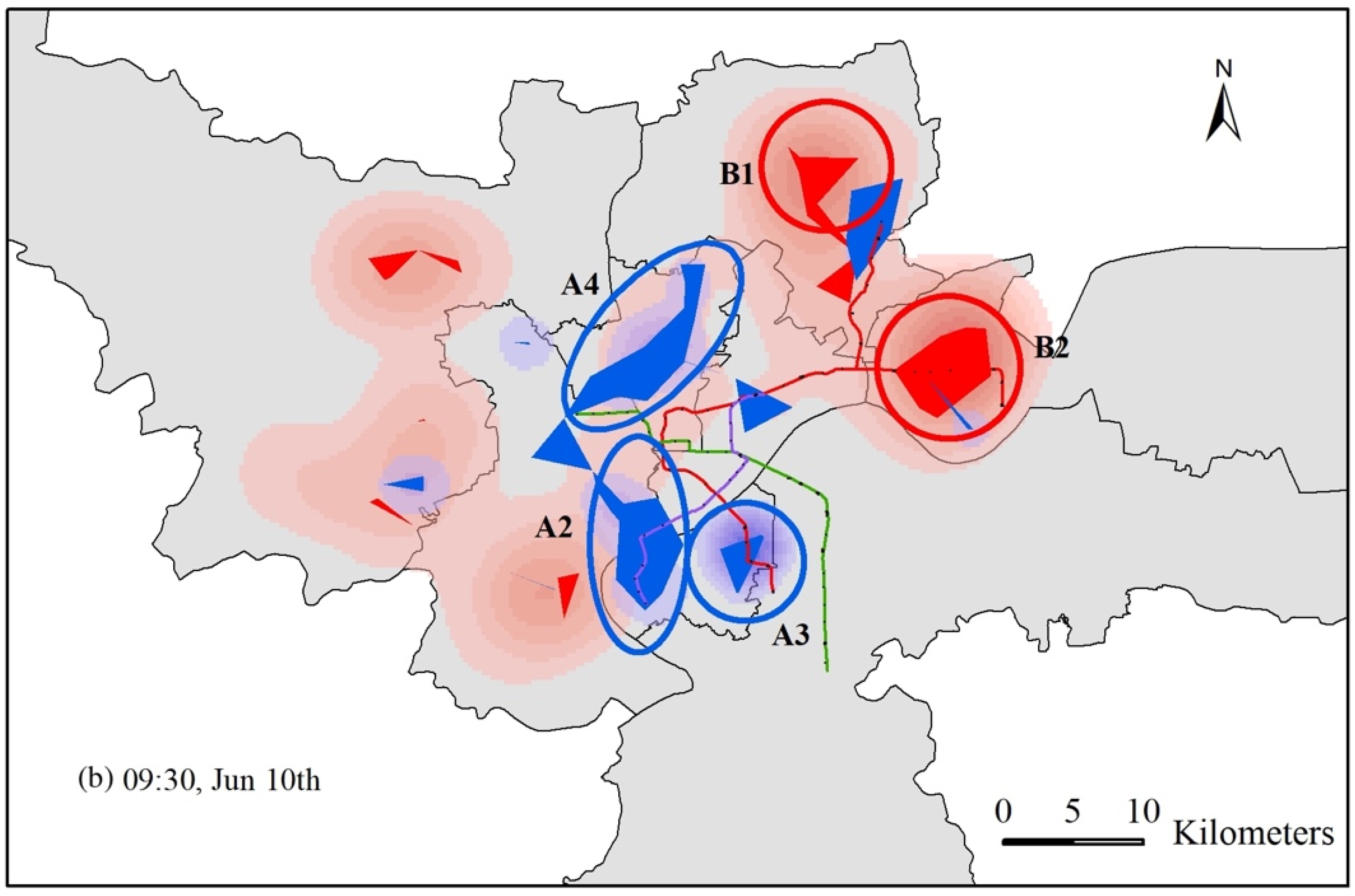
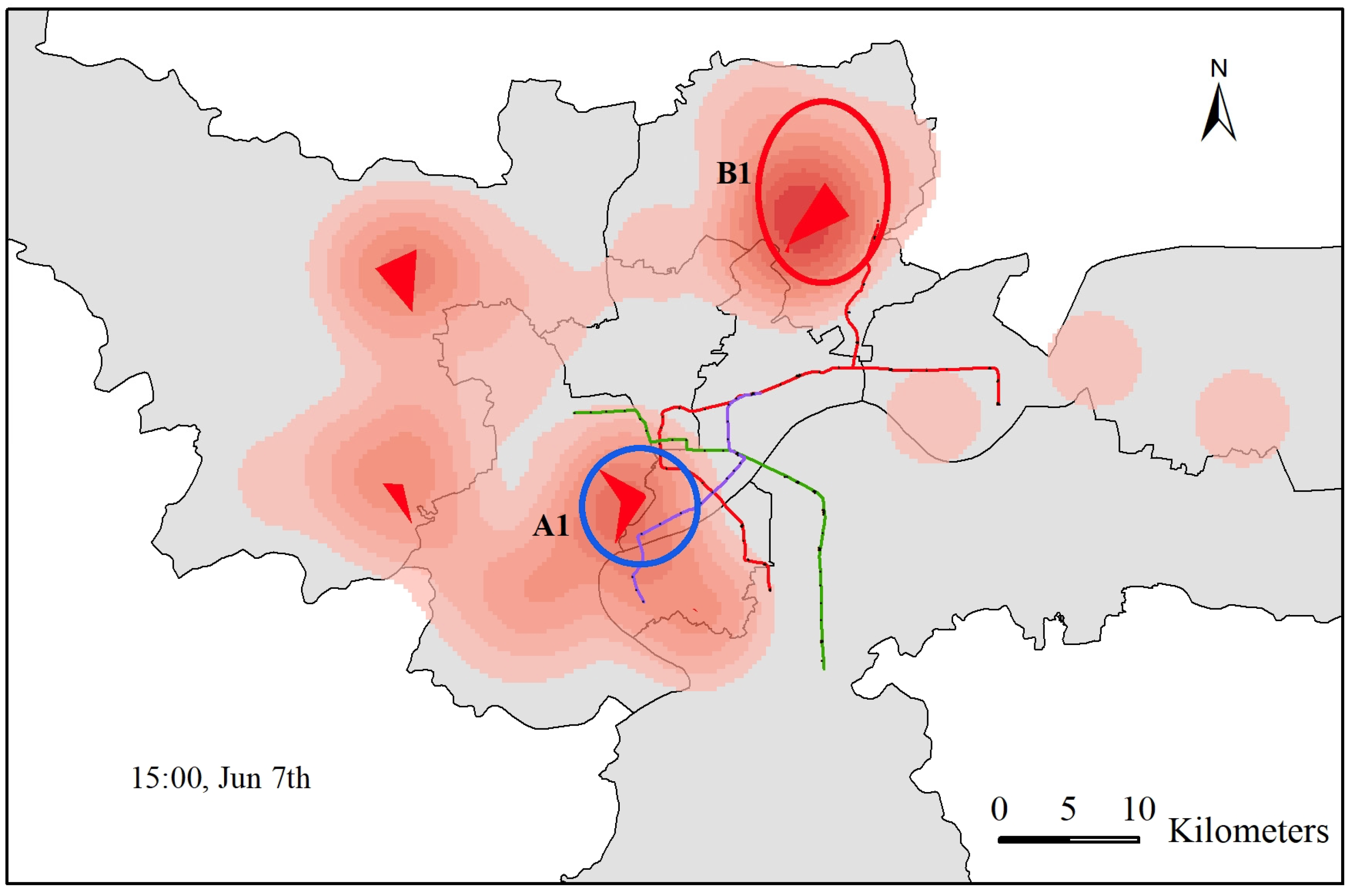
After the detection of imbalanced docking stations and the spatial filtering process, we created maps of demand conflict AOIs, shown in Figure 6 and Figure 7. Figure 6 is at 09:30 a.m., 7 June, a holiday, and 09:30 a.m. on 10 June, a weekday. In a weekday morning, Types A and B are at their local maximal value. On a holiday morning, however, Type A occurs much more widely than Type B does, implying much more scattered destinations for bicycle trips. Figure 7 is at 15:00 p.m. on 7 June, which is a local maximum for Type B on holidays. The blue area indicates a Type A imbalance usage with rental conflict and low NAB value. The red area represents the unbalanced demand of Type B, indicating that there is a conflict in demand for returning bicycles. Because of the close relationship between the metro system and the public bicycle systems in Hangzhou, metro lines and metro stations for 2019 were added, with Line 1 in red, 2 in green, and 4 in purple.
As shown in Figure 6, the locations of AOIs on weekdays and holidays are almost completely different, and imbalance usage occurs less across the city on holiday mornings than it does on the weekday mornings.
Blue AOIs (the rental conflict) in Figure 6a are located at leisure places such as the Sports Park, the Xixi Wetland, and especially the West Lake (A1). The surrounding areas of universities are clustered in blue. Compared to rental conflict, there is less pressure to return bicycles. In holiday mornings, only residential areas (B1) in the Linping district were detected with an inactive usage status.
In Figure 6b, blue AOIs (the rental conflict) are located near metro stations in the central urban area. The phenomenon is particularly noticeable in A2 and A3, where Internet enterprises and the local government of the Hangzhou high-tech zone (Binjiang) are located. This is consistent with the conclusion that the docking stations located near the company had a high rental and return amount during rush hour on weekdays [39]. The area surrounding the start station of Line 1 was also identified as a rental conflict area. In addition, the enormous cluster of the blue area (A4) in the Gongshu district covers almost all working areas and has nothing to do with metro lines. The public bicycle system meets the majority of commuting needs in this area from end to end. On the other hand, bicycle stations around universities (B2), while being on metro Line 1, show a “full” status and return conflicts.
The imbalance usage in Figure 7 is quite interesting. It shows a local maximum of Type B (return conflict) at 15:00 p.m. on 7 June. This type can be found in residential areas, including Linping (B1), Liangzhu, and Xianlin, and it is on a trend of expansion. A1 with Type A conflict changed into Type B, indicating that citizens return the bicycles and end the day’s life.
Figure 6 and Figure 7 show that imbalance usage AOIs are closely related to land use and metro stations (marked as black points). From the perspective of spatial distribution, Type A AOIs (rental conflicts) are more common in core urban areas than Type B AOIs are (return conflicts). As a result, a systematic reschedule strategy is required to ensure total balance usage. The AOI reflects areas prone to imbalance demand under the existing spatial layout, which can help the system operation department in better understanding the problem of unbalanced usage, and more appropriately completing scheduling tasks.
5. Discussion
5.1. Why Station Spacing Matters for PBS in Asian Countries
The location strategy of a public bicycle system is a critical issue of public transit since spacing between neighboring docking stations can influence the transit mode. If the coverage of public transportation is insufficient to provide convenient services, the public is more likely to choose vehicles over public bicycles, resulting in a significant decrease in the use of public bicycles. To reach more populations, PBSs in Asian countries use a small-capacity but high-densely distributed location strategy [7]. In this section, we determine a suitable station spacing value for the Hangzhou public bicycle system.
Average nearest-neighbor analysis is a typical method in geographic statistics to calculate the distance in space between each point (docking station) and its nearest neighbor. The Hangzhou public bicycle system arranges adjacent stations on roads in a two-side opposite or staggered way for the convenience of pedestrians in both directions. In this case, the average nearest-neighbor strategy yields 15.5 m, which is a smaller station spacing with significant bias about the spatial distribution of the system.
To address the issue, we designed subnearest-neighbor analysis to measure docking-station spacing. The first step is to locate all nearby stations within walking distance for each docking station. As shown in Figure 8, the target station is represented by a triangle maker, and all of its neighboring stations within walking distance are represented by red points. Second, the nearest station is removed, and the remaining, at most five, nearby stations are used to calculate the average distance. If there are no remaining nearby docking stations after removing the nearest station, we consider the target docking station to be a remote station, and use the nearest-neighbor distance as its spacing value. Lastly, we compute the average subnearest-neighbor distance and use it as the station spacing. Thus, the station spacing calculated by our subnearest-neighbor analysis was 190 m, which is more appropriate to reflect the relationship between the target docking station and its neighbors.
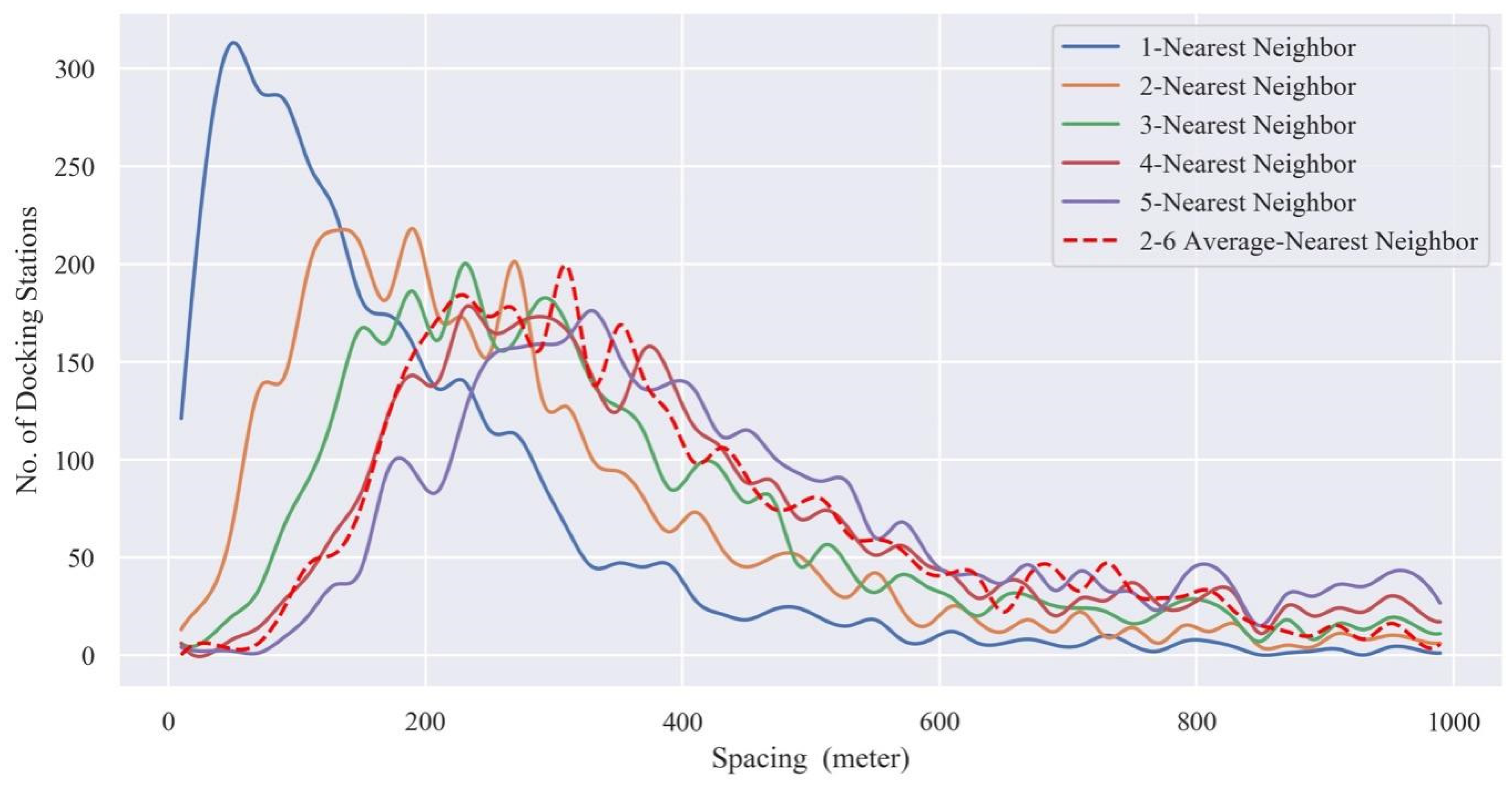
In Figure 9, the subnearest-neighbor distances of each docking station are summarized and drawn in a dashed line. The distribution of the subnearest-neighbor distance presents short-distance peaks and a long tail, avoiding the deviation of the nearest-neighbor distance (the blue curve). The three peaks are separated by three intervals, [23,24], [24,26], and [32,34]. The Guidelines for Planning and Design of Urban Pedestrian and Bicycle Transport System [40] specify a station spacing of 200 to 500 m. Although the majority of docking stations (62.8%) are in line with the station spacing specification, a significant portion of docking stations (equals to 21.1%) have neighboring stations that are more than 500 m away.
5.2. Difference before and after Using Spatial Filter
To better explain why we designed the spatial filter operator, we calculated and counted the number of problematic stations. We chose 10:00 a.m. and 15:00 p.m. on holidays, and 8:50 a.m. and 9:30 a.m. on weekdays, and followed the spatial filtering process shown in Figure 2c. The spacing between neighbors was set to 500 m. If the target station could locate any normal docking stations within the neighborhood distance, we remove it from the problematic-station list.
The total number of problematic stations before and after the spatial filtering process is shown in Table 1. Type A denotes rental conflicts, while Type B denotes return conflicts. To emphasize the importance of spatial filtering, we also calculated the ratio of real imbalance stations in each study period and present it in the table. The number of imbalanced docking stations screened only by NAB was substantial, generally exceeding 600. After spatial filtering, the identified real imbalanced docking stations accounted for nearly 7.19% of the original results detected simply by NAB.
If we set the neighbor distance to a bigger number, such as 1 km, the ratio of real imbalance stations decreases. For the majority of problematic stations, citizens can rent or return their public bicycles within walking distance. That is, the majority of the demand conflict can be alleviated by the support of adjacent docking stations without the need for intervention. Only remaining docking stations after the spatial filtering process are subject to real demand conflicts, requiring bicycle dispatching or other rebalancing strategies. Results show how the spatial filtering step can help in focusing on real imbalanced docking stations and contribute to uncovering demand conflict AOIs.
In short, taking the Hangzhou public bicycle system as an example, PBSs in Asian countries typically include walkable neighboring stations that provide citizens with alternative options. These clustering geographic relationship are considered while detecting imbalance usage. Nearby alternative stations contribute to a flexible manage system of the Hangzhou public bicycle system.
6. Conclusions
In this paper, we proposed a three-step workflow for detecting the imbalance AOIs of the Hangzhou PBS, adding a spatial filtering operation to prevent being influenced by the compact layout and neighboring stations within walking distance. Following the spatial filtering process, the majority of false-alarm stations, with an average of 92.81%, were removed and did not require rebalancing. Further, demand conflict areas were clustered and generated from the stations under real imbalance usage. The identification of imbalance AOIs can help to redesign station locations and in the better scheduling of rebalancing. For example, building new stations or providing more docking points in AOIs where imbalance usage persists can improve the level of service. Additional manual and dynamic distributed work is involved in AOIs when the main cause of imbalance usage is commuting demand in one direction.
We also analyzed the spatial configuration of the Hangzhou public bicycle system with a subnearest-neighbor method. This can effectively avoid interference from adjacent stations on the opposite side in the road. The result indicates that the majority of the station spacing of Hangzhou PBS falls in 230 to 240, 240 to 260, and 320 to 340, which is more apposite than 15.5 m by the nearest-neighbor method. The average station spacing satisfies the design guideline and is smaller than that of other PBSs globally. It emphasizes the geographic concern for neighborhood analysis of aggregated and staggered public bicycle systems, which is the basis of this studies.
The NAB is not a perfect indicator of docking station capacity. The quality of this indicator is greatly related to the trade-off between sampling frequency and usage frequency. The NAB of the docking station where bicycles are frequently rented and returned may vary as much as the NAB of a station that is rarely used [7]. However, we cannot endlessly increase sampling frequency, as too many requests damage the application system. More work is needed to address the underlying causes of conflict.
Author Contributions
Methodology, Xiaoyi Zhang; project administration, Xiaoyi Zhang; validation, Yurong Chen; visualization, Yurong Chen; writing—original draft, Xiaoyi Zhang; writing—review and editing, Yurong Chen and Yang Zhong. All authors have read and agreed to the published version of the manuscript.
Funding
This research received no external funding.
Conflicts of Interest
The authors declare no conflict of interest.
References
- Fishman, E.; Washington, S.; Haworth, N. Bike Share’s Impact on Car Use: Evidence from the United States, Great Britain, and Australia. Transp. Res. Part D Transp. Environ. 2014, 31, 13–20. [Google Scholar] [CrossRef] [Green Version]
- Shaheen, S.A.; Martin, E.W.; Cohen, A.P.; Finson, R.S. Public Bikesharing in North America: Early Operator and User Understanding; Mineta Transportation Institute: San Jose, CA, USA, 2012. [Google Scholar]
- Sato, H.; Miwa, T.; Morikawa, T. A Study on Use and Location of Community Cycle Stations. Res. Transp. Econ. 2015, 53, 13–19. [Google Scholar] [CrossRef]
- Wang, Y.; Douglas, M.; Hazen, B. Diffusion of Public Bicycle Systems: Investigating Influences of Users’ Perceived Risk and Switching Intention. Transp. Res. Part A Policy Pract. 2021, 143, 1–13. [Google Scholar] [CrossRef]
- Zhang, F.; Liu, W. An Economic Analysis of Integrating Bike Sharing Service with Metro Systems. Transp. Res. Part D Transp. Environ. 2021, 99, 103008. [Google Scholar] [CrossRef]
- Shaheen, S.A.; Cohen, A.P.; Martin, E.W. Public Bikesharing in North America: Early Operator Understanding and Emerging Trends. Transp. Res. Rec. 2013, 2387, 83–92. [Google Scholar] [CrossRef]
- O’Brien, O.; Cheshire, J.; Batty, M. Mining Bicycle Sharing Data for Generating Insights into Sustainable Transport Systems. J. Transp. Geogr. 2014, 34, 262–273. [Google Scholar] [CrossRef]
- Molina-Garcia, J.; Castillo, I.; Queralt, A.; Sallis, J.F. Bicycling to University: Evaluation of a Bicycle-Sharing Program in Spain. Health Promot. Int. 2015, 30, 350–358. [Google Scholar] [CrossRef] [Green Version]
- Li, A.; Zhao, P.; Huang, Y.; Gao, K.; Axhausen, K.W. An Empirical Analysis of Dockless Bike-Sharing Utilization and Its Explanatory Factors: Case Study from Shanghai, China. J. Transp. Geogr. 2020, 88, 102828. [Google Scholar] [CrossRef]
- Meng, S.; Brown, A. Docked vs. Dockless Equity: Comparing Three Micromobility Service Geographies. J. Transp. Geogr. 2021, 96, 103185. [Google Scholar] [CrossRef]
- Koala Growing Pains. Behind the World’s First Largest Number of Urban Public Bicycles of Chinese Cities. China Bicycl. 2015, 12, 78–81. [Google Scholar]
- Midgley, P. Bicycle-Sharing Schemes: Enhancing Sustainable Mobility in Urban Areas; United Nations, Department of Economic and Social Affairs: New York, NY, USA, 2011; Volume 8, pp. 1–12. [Google Scholar]
- Zhang, Y.; Thomas, T.; Brussel, M.; van Maarseveen, M. Exploring the Impact of Built Environment Factors on the Use of Public Bikes at Bike Stations: Case Study in Zhongshan, China. J. Transp. Geogr. 2017, 58, 59–70. [Google Scholar] [CrossRef]
- Nair, R.; Miller-Hooks, E.; Hampshire, R.C.; Bušić, A. Large-Scale Vehicle Sharing Systems: Analysis of Vélib’. Int. J. Sustain. Transp. 2013, 7, 85–106. [Google Scholar] [CrossRef] [Green Version]
- Zhou, X. Understanding Spatiotemporal Patterns of Biking Behavior by Analyzing Massive Bike Sharing Data in Chicago. PLoS ONE 2015, 10, e0137922. [Google Scholar] [CrossRef] [PubMed]
- Yu, Q.; Gu, Y.; Yang, S.; Zhou, M. Discovering Spatiotemporal Patterns and Urban Facilities Determinants of Cycling Activities in Beijing. J. Geovis. Spat. Anal. 2021, 5, 16. [Google Scholar] [CrossRef]
- Corcoran, J.; Li, T.; Rohde, D.; Charles-Edwards, E.; Mateo-Babiano, D. Spatio-Temporal Patterns of a Public Bicycle Sharing Program: The Effect of Weather and Calendar Events. J. Transp. Geogr. 2014, 41, 292–305. [Google Scholar] [CrossRef]
- Kaltenbrunner, A.; Meza, R.; Grivolla, J.; Codina, J.; Banchs, R. Urban Cycles and Mobility Patterns: Exploring and Predicting Trends in a Bicycle-Based Public Transport System. Pervasive Mob. Comput. 2010, 6, 455–466. [Google Scholar] [CrossRef]
- Chen, L.; Zhang, D.; Wang, L.; Yang, D.; Ma, X.; Li, S.; Wu, Z.; Pan, G.; Nguyen, T.-M.-T.; Jakubowicz, J. Dynamic Cluster-Based over-Demand Prediction in Bike Sharing Systems. In Proceedings of the 2016 ACM International Joint Conference on Pervasive and Ubiquitous Computing, Heidelberg, Germany, 12 September 2016; ACM: New York, NY, USA, 2016; pp. 841–852. [Google Scholar]
- Froehlich, J.E.; Neumann, J.; Oliver, N. Sensing and Predicting the Pulse of the City through Shared Bicycling. In Proceedings of the Twenty-First International Joint Conference on Artificial Intelligence, Pasadena, CA, USA, 14 July 2009. [Google Scholar]
- Wang, J.; Tsai, C.-H.; Lin, P.-C. Applying Spatial-Temporal Analysis and Retail Location Theory to Public Bikes Site Selection in Taipei. Transp. Res. Part A Policy Pract. 2016, 94, 45–61. [Google Scholar] [CrossRef]
- Li, Y.; Zheng, Y.; Zhang, H.; Chen, L. Traffic Prediction in a Bike-Sharing System. In Proceedings of the 23rd SIGSPATIAL International Conference on Advances in Geographic Information Systems, Seattle, WA, USA, 3 November 2015; ACM: New York, NY, USA, 2015; pp. 1–10. [Google Scholar]
- Vogel, P.; Greiser, T.; Mattfeld, D.C. Understanding Bike-Sharing Systems Using Data Mining: Exploring Activity Patterns. Procedia-Soc. Behav. Sci. 2011, 20, 514–523. [Google Scholar] [CrossRef] [Green Version]
- Faghih-Imani, A.; Eluru, N. Incorporating the Impact of Spatio-Temporal Interactions on Bicycle Sharing System Demand: A Case Study of New York CitiBike System. J. Transp. Geogr. 2016, 54, 218–227. [Google Scholar] [CrossRef]
- Ye, X.; Du, J.; Gong, X.; Zhao, Y.; AL-Dohuki, S.; Kamw, F. SparseTrajAnalytics: An Interactive Visual Analytics System for Sparse Trajectory Data. J. Geovis. Spat. Anal. 2021, 5, 3. [Google Scholar] [CrossRef]
- Liu, F.; Andrienko, G.; Andrienko, N.; Chen, S.; Janssens, D.; Wets, G.; Theodoridis, Y. Citywide Traffic Analysis Based on the Combination of Visual and Analytic Approaches. J. Geovis. Spat. Anal. 2020, 4, 15. [Google Scholar] [CrossRef]
- Maleki Vishkaei, B.; Mahdavi, I.; Mahdavi-Amiri, N.; Khorram, E. Balancing Public Bicycle Sharing System Using Inventory Critical Levels in Queuing Network. Comput. Ind. Eng. 2020, 141, 106277. [Google Scholar] [CrossRef]
- Patel, S.J.; Patel, C.R. A Stakeholders Perspective on Improving Barriers in Implementation of Public Bicycle Sharing System (PBSS). Transp. Res. Part A Policy Pract. 2020, 138, 353–366. [Google Scholar] [CrossRef]
- Borgnat, P.; Abry, P.; Flandrin, P.; Robardet, C.; Rouquier, J.-B.; Fleury, E. Shared bicycles in a city: A signal processing and data analysis perspective. Adv. Complex Syst. 2011, 14, 415–438. [Google Scholar] [CrossRef] [Green Version]
- Fricker, C.; Gast, N. Incentives and Redistribution in Homogeneous Bike-Sharing Systems with Stations of Finite Capacity. EURO J. Transp. Logist. 2016, 5, 261–291. [Google Scholar] [CrossRef] [Green Version]
- O’Mahony, E.; Shmoys, D. Data Analysis and Optimization for (Citi)Bike Sharing. In Proceedings of the AAAI Conference on Artificial Intelligence, Austin, TX, USA, 25–30 February 2015; Volume 29. [Google Scholar]
- Ciancia, V.; Latella, D.; Massink, M.; Pakauskas, R. Exploring Spatio-Temporal Properties of Bike-Sharing Systems. In Proceedings of the 2015 IEEE International Conference on Self-Adaptive and Self-Organizing Systems Workshops, Cambridge, MA, USA, 21 September 2015; IEEE: Piscataway, NJ, USA, 2015; pp. 74–79. [Google Scholar]
- Qian, J.; Zheng, Z.; Feng, Y. An Assessment of the Public Bicycle Facilities in Hangzhou. Planners 2010, 26, 71–76. [Google Scholar]
- Shaheen, S.A.; Guzman, S.; Zhang, H. Bikesharing in Europe, the Americas, and Asia: Past, Present, and Future. Transp. Res. Rec. 2010, 2143, 159–167. [Google Scholar] [CrossRef] [Green Version]
- Yao, Y.; Zhou, Y. Bike Sharing Planning System in Hangzhou. Urban Transp. China 2009, 7, 30–38. [Google Scholar]
- Wang, S.; Zhang, J.; Liu, L.; Duan, Z. Bike-Sharing-A New Public Transportation Mode: State of the Practice & Prospects. In Proceedings of the 2010 IEEE International Conference on Emergency Management and Management Sciences, Beijing, China, 8–10 August 2010; IEEE: Piscataway, NJ, USA, 2010; pp. 222–225. [Google Scholar]
- Hangzhou Public Bicycle Transportation Service Development Co., Ltd. Bicycle Service. Available online: http://www.ggzxc.cn/ (accessed on 1 February 2019).
- Li, J.; Wang, F. Characteristics of Bike Sharing Service in Hangzhou Based on Open Data. Urban Transp. China 2017, 15, 63–73. [Google Scholar]
- Shi, X.; Yu, Z.; Chen, J.; Xu, H.; Lin, F. The Visual Analysis of Flow Pattern for Public Bicycle System. J. Vis. Lang. Comput. 2018, 45, 51–60. [Google Scholar] [CrossRef]
- Ministry of Housing and Urban-Rural Development. Guidelines for Planning and Design of Urban Pedestrian and Bicycle Transport System. 2013. Available online: http://www.mohurd.gov.cn/wjfb/201401/t20140114_216859.html (accessed on 16 September 2021).
Figure 1.
Hangzhou public bicycle system in 2019. The administrative boundary of Hangzhou changed in 2020.
Figure 1.
Hangzhou public bicycle system in 2019. The administrative boundary of Hangzhou changed in 2020.

Figure 2.
Three-step workflow of demand conflict detection and AOI delineation. (a) The results of status calculation; (b) spatial filtering process; (c) the results after spatial filtering and (d) the result imbalance AOI.
Figure 2.
Three-step workflow of demand conflict detection and AOI delineation. (a) The results of status calculation; (b) spatial filtering process; (c) the results after spatial filtering and (d) the result imbalance AOI.
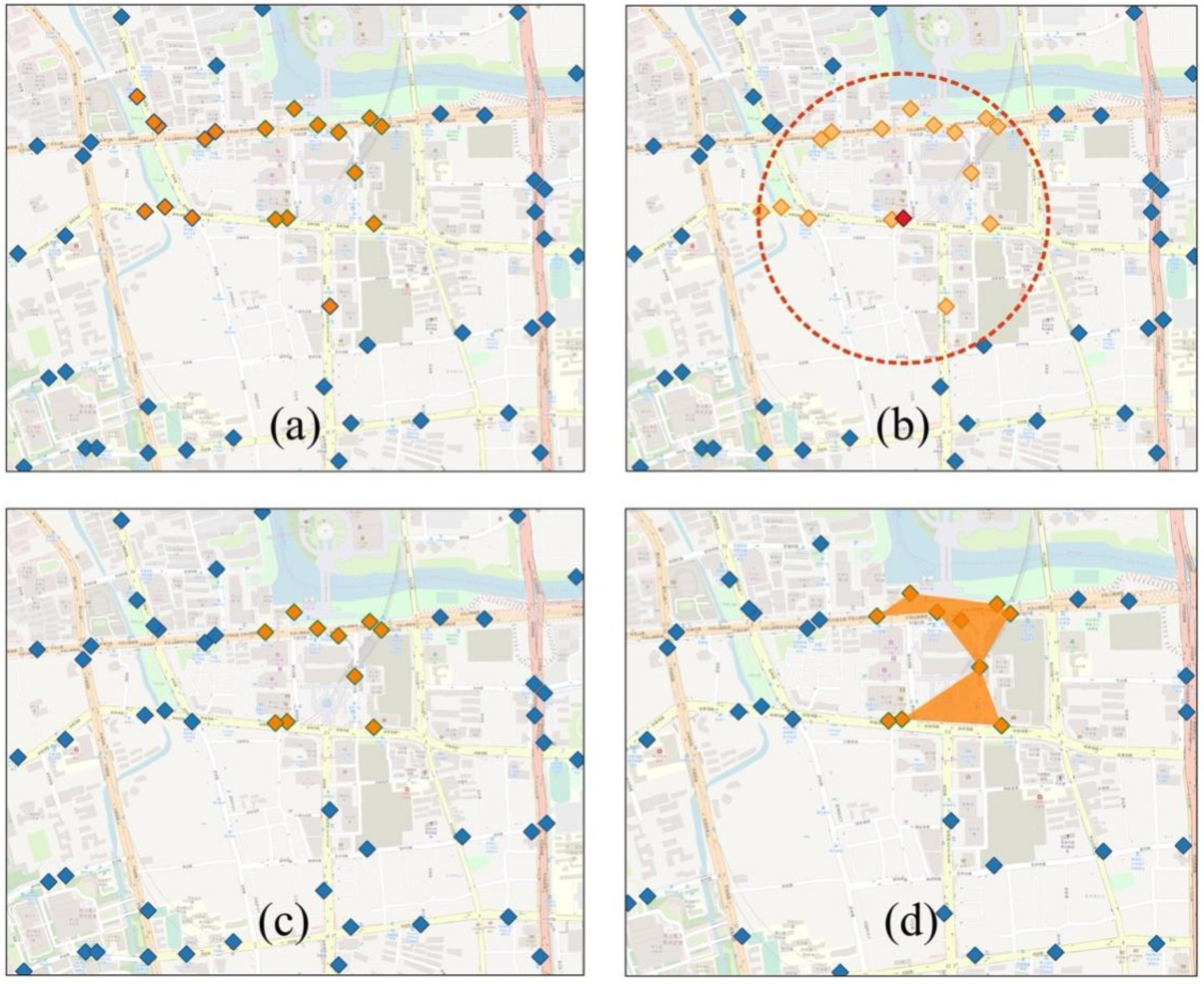
Figure 3.
Change in NAB of Hangzhou public bicycle system on typical days.
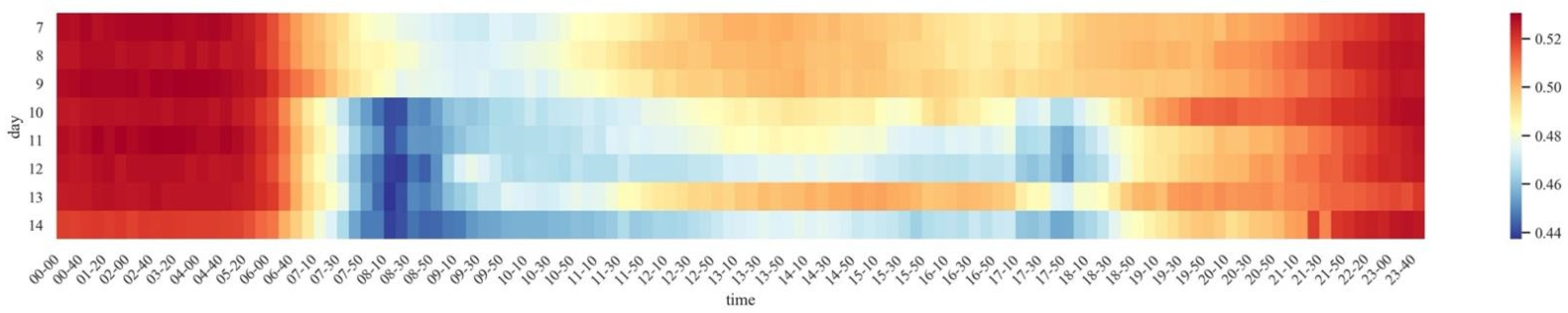
Figure 4.
Sensitive analysis on imbalance usage detection. Fit results on the number of (a) type A and (b) type B stations.
Figure 4.
Sensitive analysis on imbalance usage detection. Fit results on the number of (a) type A and (b) type B stations.

Figure 5.
Statistical result of demand conflict. Red line, NAB higher than 0.74; blue line, NAB lower than 0.25.
Figure 5.
Statistical result of demand conflict. Red line, NAB higher than 0.74; blue line, NAB lower than 0.25.

Figure 6.
Distribution of imbalance usage areas (AOIs) on (a) top: holiday mornings and (b) bottom: weekday mornings.
Figure 6.
Distribution of imbalance usage areas (AOIs) on (a) top: holiday mornings and (b) bottom: weekday mornings.


Figure 7.
Distribution of imbalance usage areas (AOIs) on holiday afternoon.

Figure 8.
Subnearest-neighbor analysis.
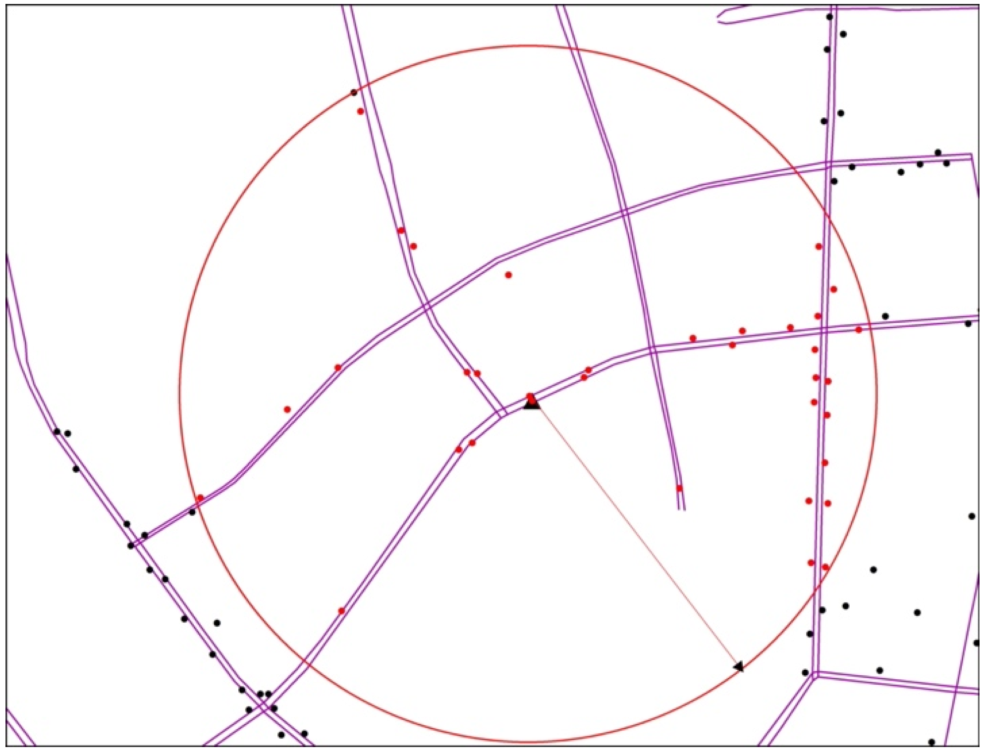
Figure 9.
Spacing between docking stations with k-nearest neighbor and subnearest neighbor.

Table 1.
Detection result of imbalanced docking stations.
| Time | Conflict Type | Before Spatial Filtering | After Spatial Filtering | Ratio |
|---|---|---|---|---|
| 10:00 a.m. 7 June 2019 | A | 934 | 46 | 4.93% |
| 15:00 p.m. 7 June 2019 | B | 626 | 38 | 6.07% |
| 10:00 a.m. 8 June 2019 | A | 881 | 35 | 3.97% |
| 15:00 p.m. 8 June 2019 | B | 590 | 36 | 6.10% |
| 10:00 a.m. 9 June 2019 | A | 894 | 46 | 5.15% |
| 15:00 p.m. 9 June 2019 | B | 593 | 46 | 7.76% |
| 08:50 a.m. 10 June 2019 | A | 1121 | 90 | 8.03% |
| 09:30 a.m. 10 June 2019 | B | 664 | 61 | 9.19% |
| 08:50 a.m. 11 June 2019 | A | 1096 | 90 | 8.21% |
| 09:30 a.m. 11 June 2019 | B | 648 | 53 | 8.18% |
| 08:50 a.m. 12 June 2019 | A | 1092 | 76 | 6.96% |
| 09:30 a.m. 12 June 2019 | B | 633 | 53 | 8.37% |
| 08:50 a.m. 13 June 2019 | A | 1076 | 99 | 9.20% |
| 09:30 a.m. 13 June 2019 | B | 639 | 53 | 8.29% |
| 08:50 a.m. 14 June 2019 | A | 1139 | 82 | 7.20% |
| 09:30 a.m. 14 June 2019 | B | 631 | 47 | 7.45% |
Publisher’s Note: MDPI stays neutral with regard to jurisdictional claims in published maps and institutional affiliations. |
© 2021 by the authors. Licensee MDPI, Basel, Switzerland. This article is an open access article distributed under the terms and conditions of the Creative Commons Attribution (CC BY) license (https://creativecommons.org/licenses/by/4.0/).
Share and Cite
MDPI and ACS Style
Zhang, X.; Chen, Y.; Zhong, Y. Spatial and Temporal Characteristic Analysis of Imbalance Usage in the Hangzhou Public Bicycle System. ISPRS Int. J. Geo-Inf. 2021, 10, 637. https://doi.org/10.3390/ijgi10100637
AMA Style
Zhang X, Chen Y, Zhong Y. Spatial and Temporal Characteristic Analysis of Imbalance Usage in the Hangzhou Public Bicycle System. ISPRS International Journal of Geo-Information. 2021; 10(10):637. https://doi.org/10.3390/ijgi10100637
Chicago/Turabian StyleZhang, Xiaoyi, Yurong Chen, and Yang Zhong. 2021. "Spatial and Temporal Characteristic Analysis of Imbalance Usage in the Hangzhou Public Bicycle System" ISPRS International Journal of Geo-Information 10, no. 10: 637. https://doi.org/10.3390/ijgi10100637
Note that from the first issue of 2016, this journal uses article numbers instead of page numbers. See further details here.