
Application of Neural Networks to Classification of Data of the TUS Orbital Telescope


D.V. Skobeltsyn Institute of Nuclear Physics, M.V. Lomonosov Moscow State University, 119991 Moscow, Russia
Universe 2021, 7(7), 221; https://doi.org/10.3390/universe7070221
Submission received: 31 May 2021
/
Revised: 25 June 2021
/
Accepted: 26 June 2021
/
Published: 1 July 2021
(This article belongs to the Special Issue New Frontiers in Astroparticle Physics: From Nuclear Reactions to Multimessenger Astronomy)
Abstract
:We employ neural networks for classification of data of the TUS fluorescence telescope, the world’s first orbital detector of ultra-high energy cosmic rays. We focus on two particular types of signals in the TUS data: track-like flashes produced by cosmic ray hits of the photodetector and flashes that originated from distant lightnings. We demonstrate that even simple neural networks combined with certain conventional methods of data analysis can be highly effective in tasks of classification of data of fluorescence telescopes.
1. Introduction
It is well known that charged particles in an extensive air shower generated by a cosmic ray hitting the Earth’s atmosphere interact with atmospheric nitrogen, causing it to emit ultraviolet (UV) light via a process called fluorescence. Registration of this UV emission in the nocturnal atmosphere with dedicated telescopes is an established technique of studies in the field of ultra-high energy cosmic rays (UHECRs) that demonstrated its efficacy with the Fly’s Eye detector array in 1980–1993 [1]. Presently fluorescence telescopes are an inherent part of both main modern experiments dedicated to such studies—the Pierre Auger Observatory [2] and the Telescope Array [3] complementing their surface detectors.
One of the main problems in UHECR studies is their extremely low flux at energies ≳5 eV, above the so-called Greisen–Zatsepin–Kuzmin cut-off [4,5]. This necessitates running ground experiments occupying huge areas. For example, the Pierre Auger Observatory covers an area of ∼3000 . In the early 1980s, Benson and Linsley suggested to increase dramatically the exposure of UHECR experiments by a totally different approach. They suggested to put a wide-field-of view fluorescence telescope into a low-Earth orbit and employ it for registering fluorescence and Cherenkov emission of extensive air showers born by UHECRs in the nocturnal atmosphere [6,7].
Several projects aimed to implement the idea of Benson and Linsley have been suggested since then, among them Orbiting Wide-field Light-collectors (OWL) [8], Tracking Ultraviolet Setup (TUS) and KLYPVE (Kosmicheskie Luchi Predel’no Vysokikh Energii, which stands for Extreme Energy Cosmic Rays in Russian) [9,10], the former Extreme Universe Space Observatory on board the Japanese Experiment Module, now Joint Experiment Missions for Extreme Universe Space Observatory (JEM-EUSO) [11] and others. TUS was the first one launched into space in 2016 [12]. It was a comparatively simple device designed as a prototype of the KLYPVE project. Its main aim was to test the technique suggested by Benson and Linsley. The data set obtained with TUS has demonstrated that an unexpected variety of different processes are taking place in the nocturnal atmosphere of the Earth in the ultraviolet (UV) range. Considerable efforts have been put in the analysis of the TUS data, see, e.g., [13,14,15,16,17]. Until recently, all of them were based on conventional approaches. Results of the first attempt of classifying the TUS data with neural networks were briefly presented in [18]. The work was motivated by several reasons. On the one hand, TUS registered more than 78 thousand events in the main mode of operation aimed at observing the fastest phenomena in the atmosphere, and more than almost 12 thousand events in other modes, with every event represented by 65,536 numbers. A visual analysis of this data set is a time-taking and error-prone process, which must be supported by established methods of data analysis. On the other hand, methods that involve machine learning and neural networks are ubiquitous presently in many branches of science and everyday life but their application in the field of cosmic ray physics is still rather limited, see a few examples in [19,20,21,22,23,24,25,26] for a brief review.
The Mini-EUSO fluorescence telescope developed by the JEM-EUSO collaboration is currently working onboard the International Space Station [27], a stratospheric experiment EUSO-SPB2 equipped with a fluorescence and a Cherenkov telescopes is to be launched in 2023 [28] and an advanced POEMMA (Probe Of Extreme Multi-Messenger Astrophysics) mission consisting of two orbital telescopes aimed at registering UHE cosmic rays and neutrinos is being developed [29]. The spatial resolution and the amount of data of these experiments is expected to be orders of magnitude bigger than that of TUS. This suggests developing methods suitable for an analysis of their data, including methods based on neural networks. The work [18] was the first step in this direction applied to the TUS data. In the present paper, we further develop the approach suggested in [18] and present more results of applying neural networks to classification of data of the TUS mission. All neural networks were implemented in Python with the Keras library [30] available in TensorFlow [31].
2. The TUS Detector
A comprehensive description of the TUS telescope can be found in [12,32]. Here we will briefly outline its main features important for the article.
From the very beginning TUS, was designed as a simple device, a pathfinder for a much more sophisticated KLYPVE experiment onboard the International Space Station [9,10]. The main components of TUS were a Fresnel mirror and a square-shaped photodetector aligned to the focal surface of the mirror. The mirror had an area of nearly 2 and a 1.5 m focal distance. The field of view (FOV) of the telescope was , which covered an area of approximately at sea level. Two hundred 56 Hamamatsu R1463 photomultiplier tubes (PMTs) formed the focal surface of the photodetector. A glass UV filter was placed in front of every PMT to limit the measured wavelength to the 300–400 nm range. Light guides with square entrance apertures and circular outputs were used to uniformly fill the FOV. All pixels had 1 cm black blends to protect them from side illumination but the telescope as a whole did not have any side shields.
All pixels were grouped in 16 modules, each of which had its own high-voltage power supply and a data processing system for the first-level trigger. The high-voltage system (HVS) was aimed to adjust the sensitivity of PMTs to the intensity of the incoming light and switch them off completely on day sides of the orbit.
The TUS electronics could operate in four modes with different time sampling windows. The main mode was intended for registering the fastest processes in the atmosphere and had the time step of 0.8 μs. Every record consisted of ADC codes written for all photodetector channels in 256 time steps with a total duration of 204.8 μs. We only discuss events registered in this mode of operation.
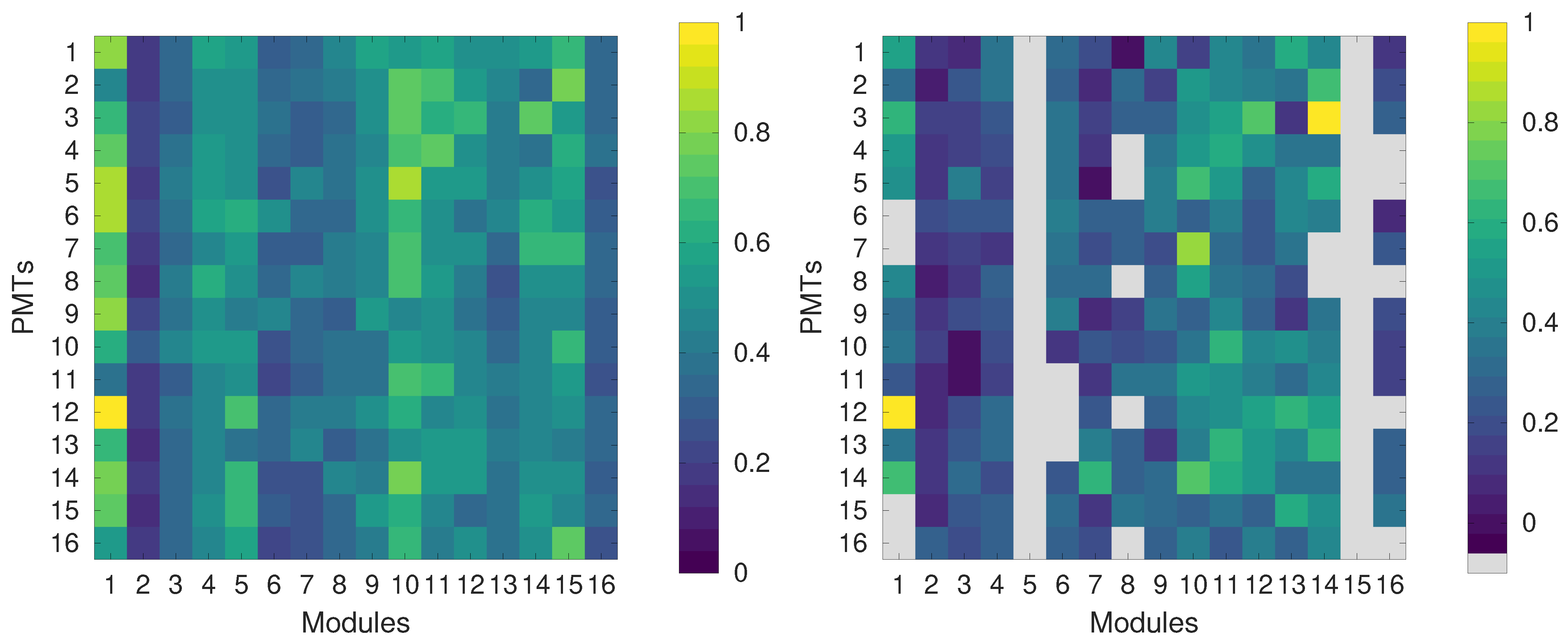
TUS was launched into orbit on 28 April 2016, as a part of the scientific payload of the Lomonosov satellite. The satellite had a sun-synchronous orbit with an inclination of , a height about 470–515 km and a period of ≈94 min. The detector was first put into operation on 19 May 2016. Unfortunately, a shortcut took place in the HVS of the photodetector at the very first day of operation [16]. Due to this, the device operated at the highest voltage during the first few orbits, including day segments, until information about this arrived at the operating center and the detector was switched off. As a result of the accident, the HVSs of two modules were burnt and these modules did not operate anymore. In other modules, PMTs with a high current were damaged. Totally, 51 photodetector channels were burnt. They are shown in grey in the right panel of Figure 1. Besides this, sensitivities of other channels changed.
Several attempts to perform an in-flight calibration of the photodetector have been made [16,33]. These methods, as well as a method tested during the present work (see Section 3.2), resulted in estimates of relative sensitivities that qualitatively agreed with each other for the majority of channels. Figure 1 shows relative sensitivities of photodetector channels calculated from the pre-flight calibration and estimated after the mission. However, none of the approaches has provided reliable estimations of absolute PMT gains. More than this, all estimates of relative sensitivities of photodetector channels were obtained for the highest codes of the HVS, which correspond to perfect observational conditions, but only 38.4% of data satisfy this criterion. Together with a few changes of the trigger settings made during the mission, this poses certain problems for the data analysis within a unified approach.
Regular operation of TUS began on 18 August 2016, and continued till 30 November 2017.
3. Phenomenological Classification of the TUS Data
A preliminary phenomenological classification of TUS events was ready by October 2016 [13] and was refined later on [12]. All events were divided into several groups:
- events with stationary noise-like waveforms; these included events with a strongly non-uniform illumination of the focal surface with bright regions correlated with geographical positions of cities and objects such as airports, power plants, offshore platforms etc.
- instant track-like flashes (TLFs) caused by charged particles hitting the UV filters of the photodetector;
- flashes produced by light coming outside of the FOV of the detector and scattered on its mirror; they were called “slow flashes” because of the long signal rise time in comparison with TLFs; and
- events with complex spatio-temporal dynamics; these included so-called ELVEs, which are short-lived optical events that manifest at the lower edge of the ionosphere (altitudes of ∼90 km) as bright rings expanding at the speed of light up to a maximum radius of ∼300 km [34], events with waveforms that could be expected from fluorescence originating from extensive air showers produced by extreme energy cosmic rays, as well as violent flashes of a yet unknown origin.
Miscellaneous examples of events of all types can be found in [12,13,14,15,16,17]. Please note that the four classes of events were not disjoint: in some cases an event of one type was registered simultaneously with an event of another type within one data record. In what follows, we shall focus on instant track-like flashes and slow flashes. Let us recall their main features before discussing an application of neural networks for their search.
3.1. Instant Track-Like Flashes
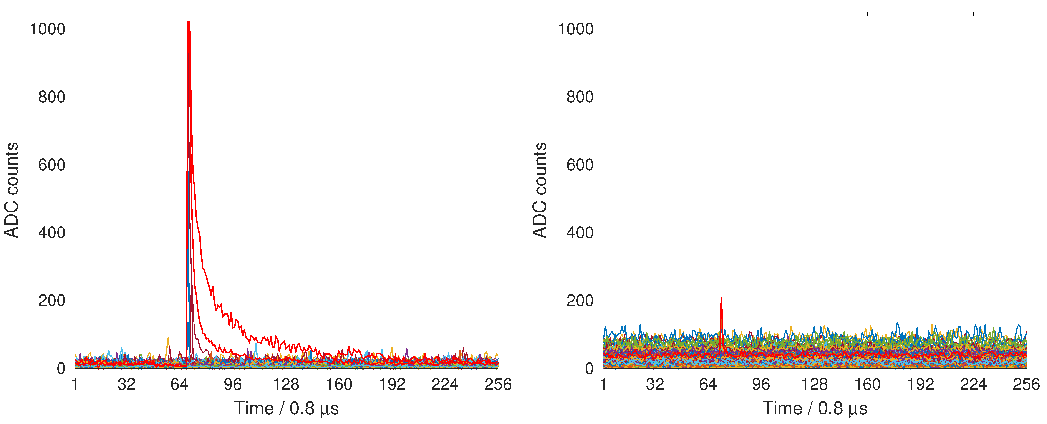
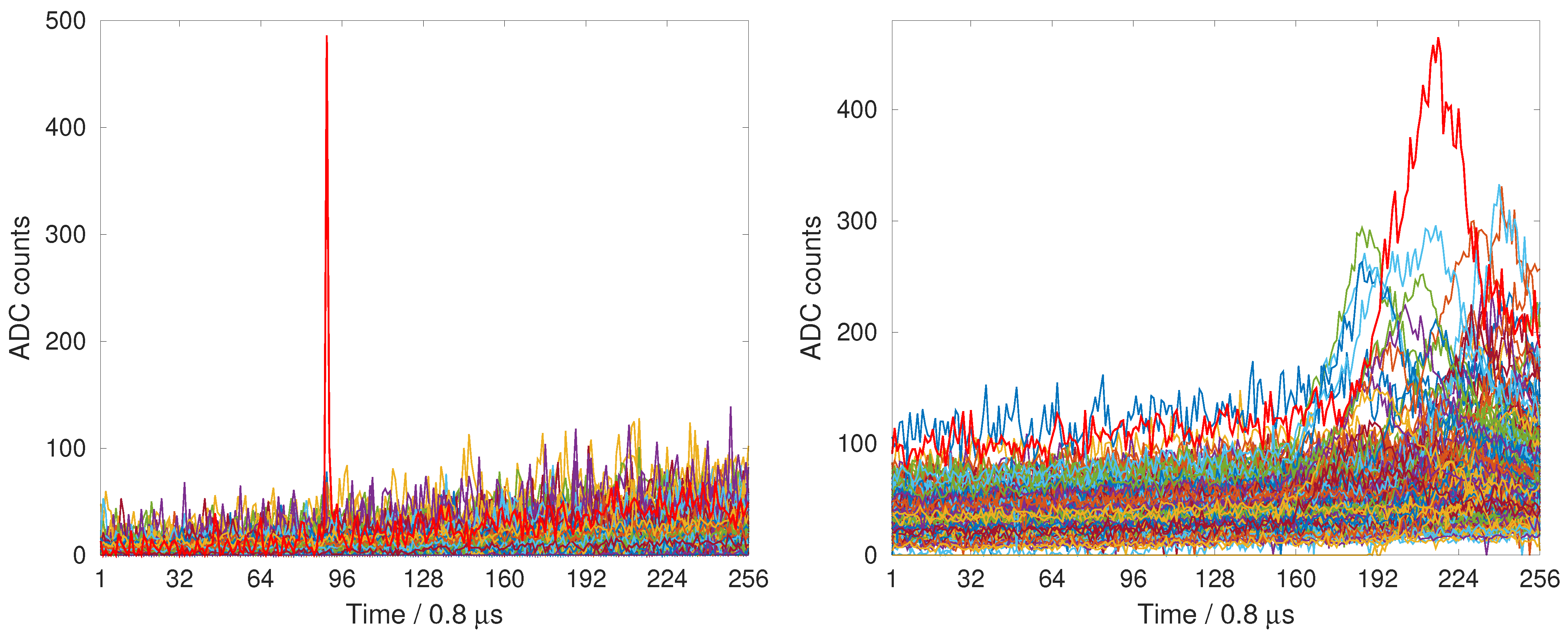
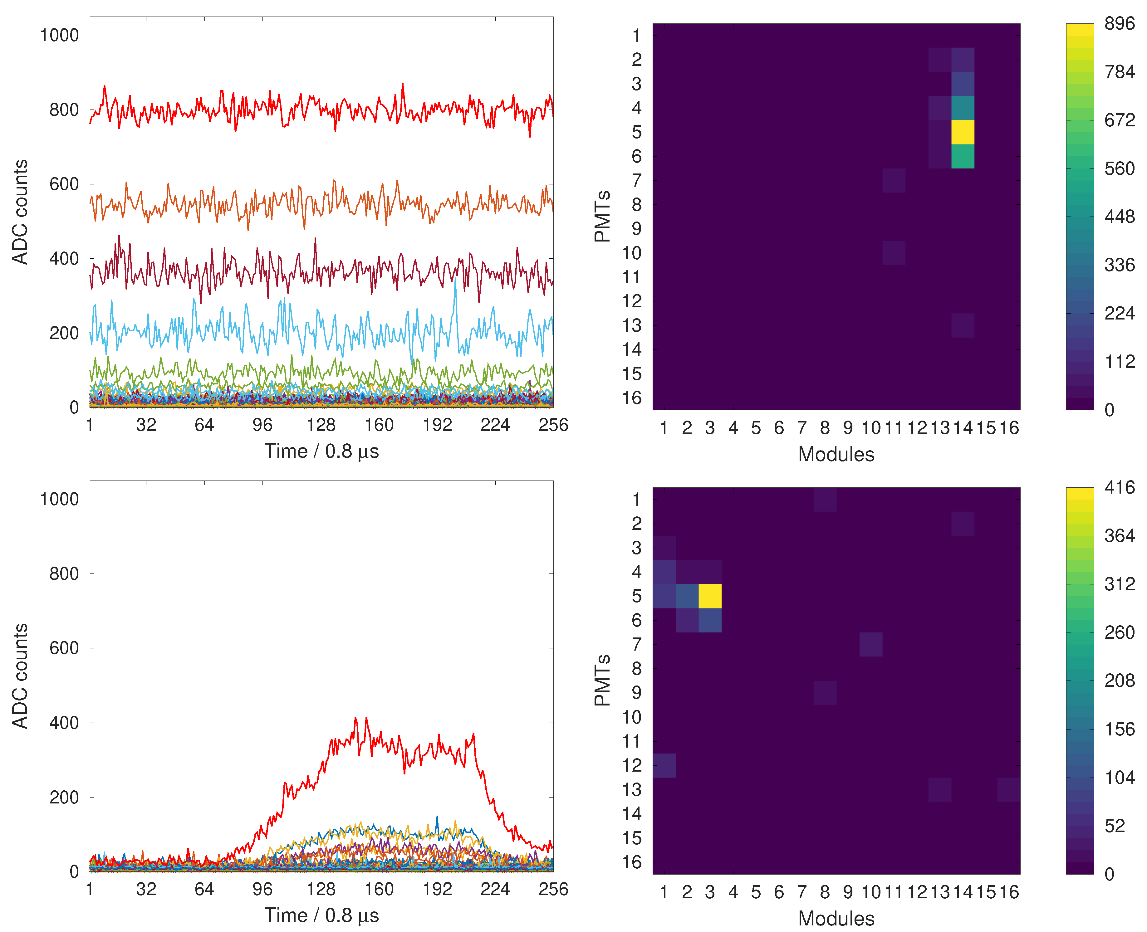
TLFs were observed in the TUS data from the very beginning of the mission on 19 May 2016. They demonstrated an instant growth of the signal (in one or two time steps), mostly to the highest possible ADC codes, in a single pixel or a group of pixels, sometimes producing a kind of a linear track on the focal surface. Therefore, they were called “instant track-like flashes”. They comprised about 10% in average of all events and up to 25% during moonless nights before they were suppressed in late April 2017, with an update of the onboard software. A typical shape of a TLF is shown on the left panel of Figure 2. However, their signals were dim in some cases as demonstrated on the right panel of Figure 2.
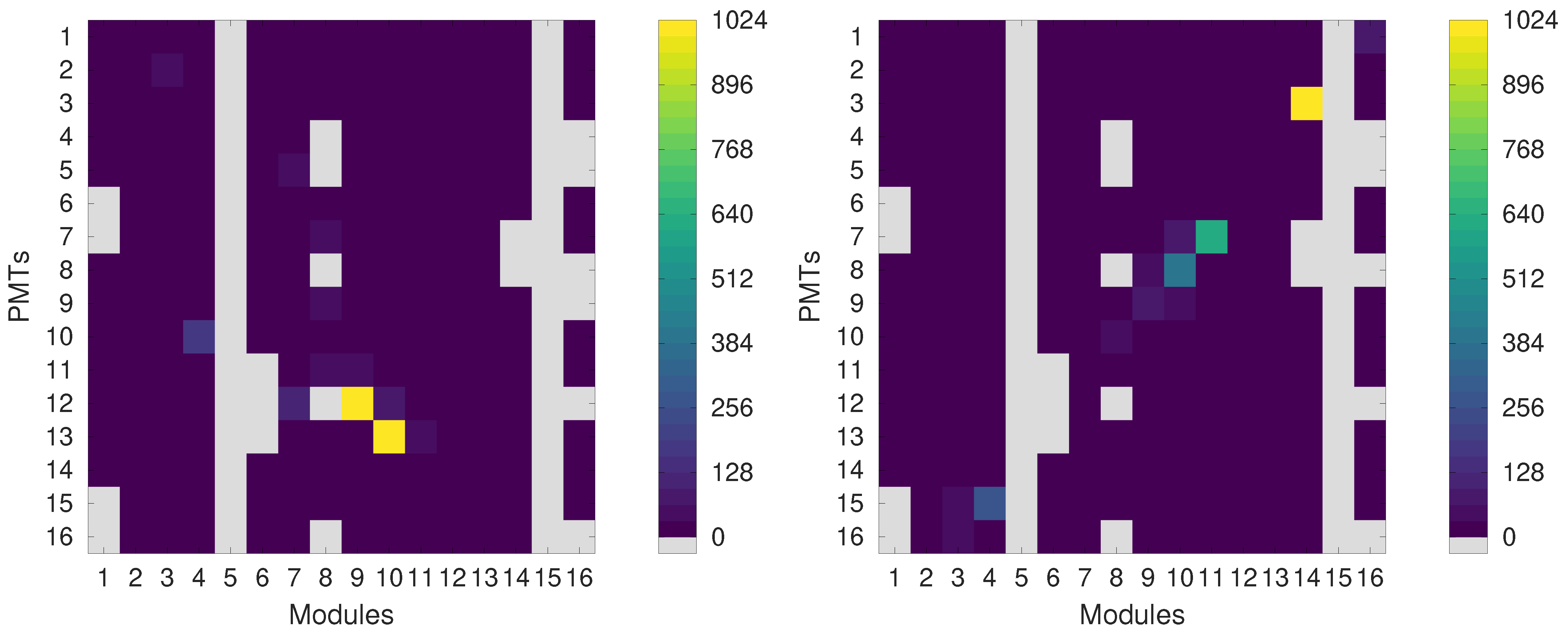
Although waveforms of TLFs could be easily selected by eye in the majority of cases, their traces on the focal surface were much more diverse. Figure 3 provides a couple of examples of events in which clear linear tracks could be seen in the focal surface. In other cases, the traces of TLFs were not that evident. A few typical examples are provided in Figure 4, Figure 5 and Figure 6.
In many cases, TLFs produced a signal in a small group or even in a single channel of the focal surface creating a spot-like trace similar those shown in Figure 4. This could take place both for weak flashes with a low amplitude and for flashes that saturated the channels as shown in the figure.
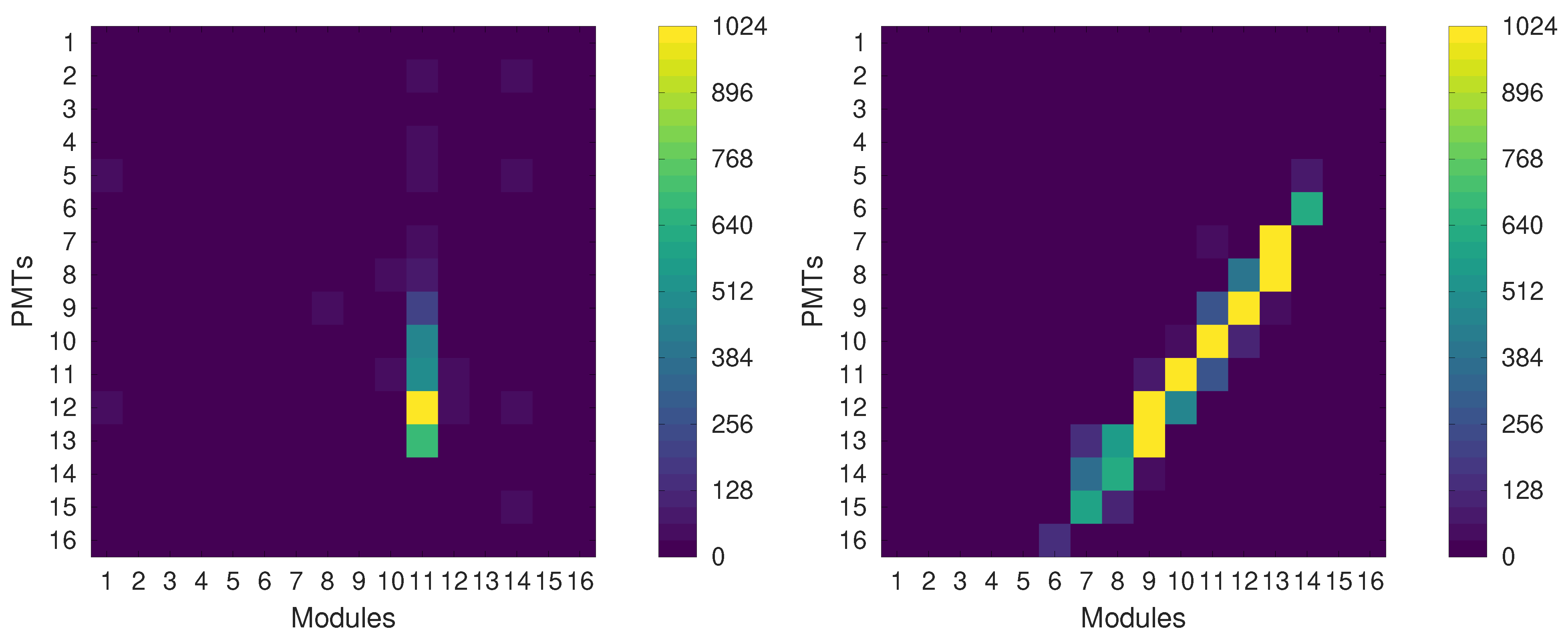
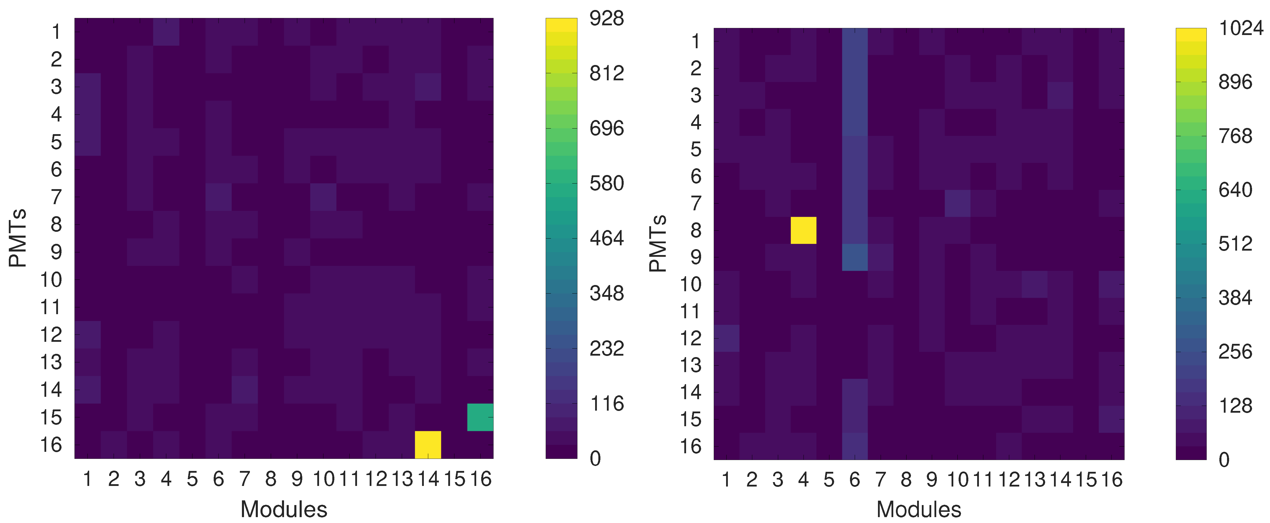
Figure 5 presents two examples of linear traces broken by passing through inactive or low-sensitivity channels. In the left panel, a track spanning through seven modules is clearly broken when intersecting several dead channels. The situation is more complex for the event shown in the right panel. The track spans from PMT 1 in module 16 to PMT 16 in module 3. It crosses two dead modules, a group of dead PMTs in module 6 and several low-sensitivity channels in modules 7, 8 and 9, cf. the right panel of Figure 1. Besides this, the instant growth of the signal in modules 12 and 13 is recorded one time step later due to the way ADC codes were read out. As a result, we obtain a “dashed” track. That was a typical situation since 51 channels were dead (i.e., almost 20% of the focal surface), and PMT gains of a whole number of channels decreased drastically after the misbehavior of the HV system discussed in Section 2.
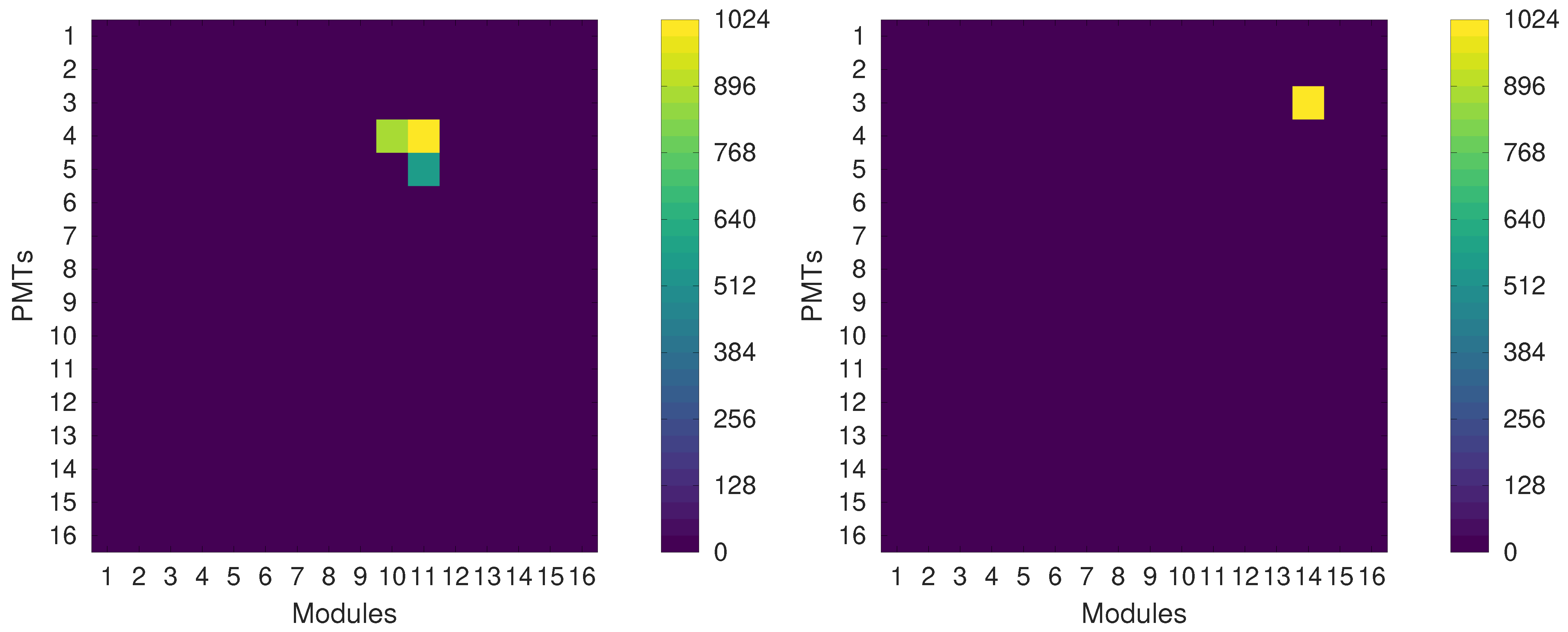
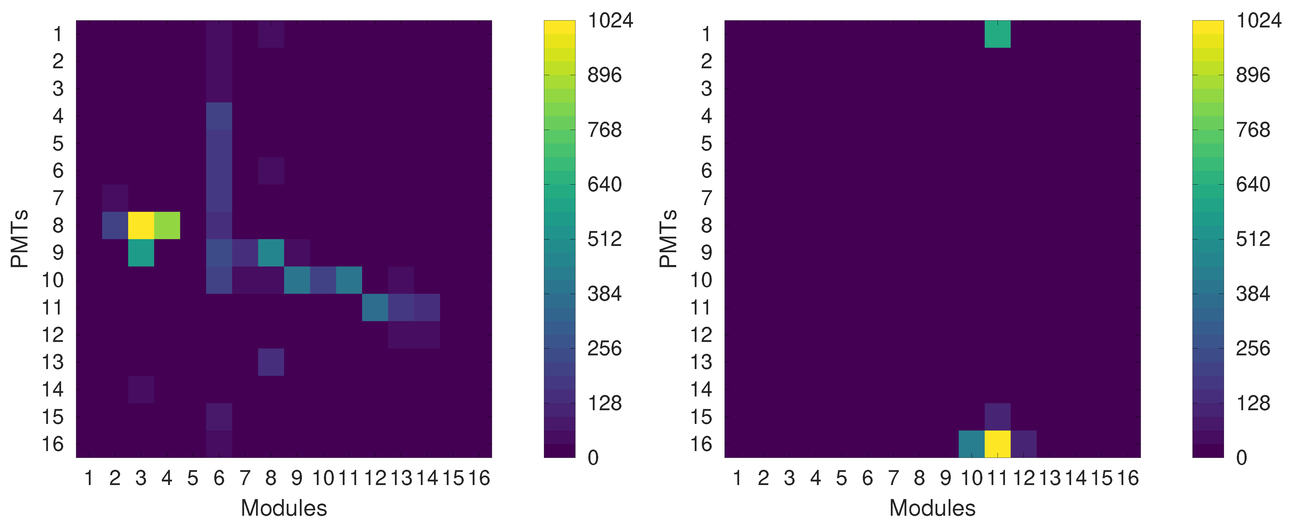
Figure 6 provides two examples of situations when a signal of a TLF was distorted due to some peculiarities in the work of onboard electronics. An X-shaped trace shown in the left panel originated because of a crosstalk in module 6. A situation such as this used to occur mostly with module 6 but could also be found in a less pronounced form with module 8. The right panel of Figure 6 presents an example of a TLF that took place at the edge of the focal surface at one end of a module and produced a simultaneous signal in a channel at the opposite side of the active module.
Understanding the nature of TLFs was straightforward since long tracks in the focal surface appearing in less than a microsecond could not be produced by flashes in the atmosphere. A simulation performed with GEANT4 [35] confirmed that such signals could be produced by protons with energies in the range from a few hundred MeV to several GeV hitting the photodetector (mostly the UV filters) [36]. An analysis of the latitudinal distribution of TLFs also supported this hypothesis [12].
TLFs presented a class of “parasitic” events that occupied a part of active time of the detector. An anti-trigger was implemented in the onboard software on 28 April 2017, which effectively reduced their number in the TUS data by an order of magnitude.
3.2. Slow Flashes
As already mentioned above, slow flashes were named as such due to the long signal rise time in comparison with TLFs. Similar to TLFs, they are ubiquitous in the TUS data set.
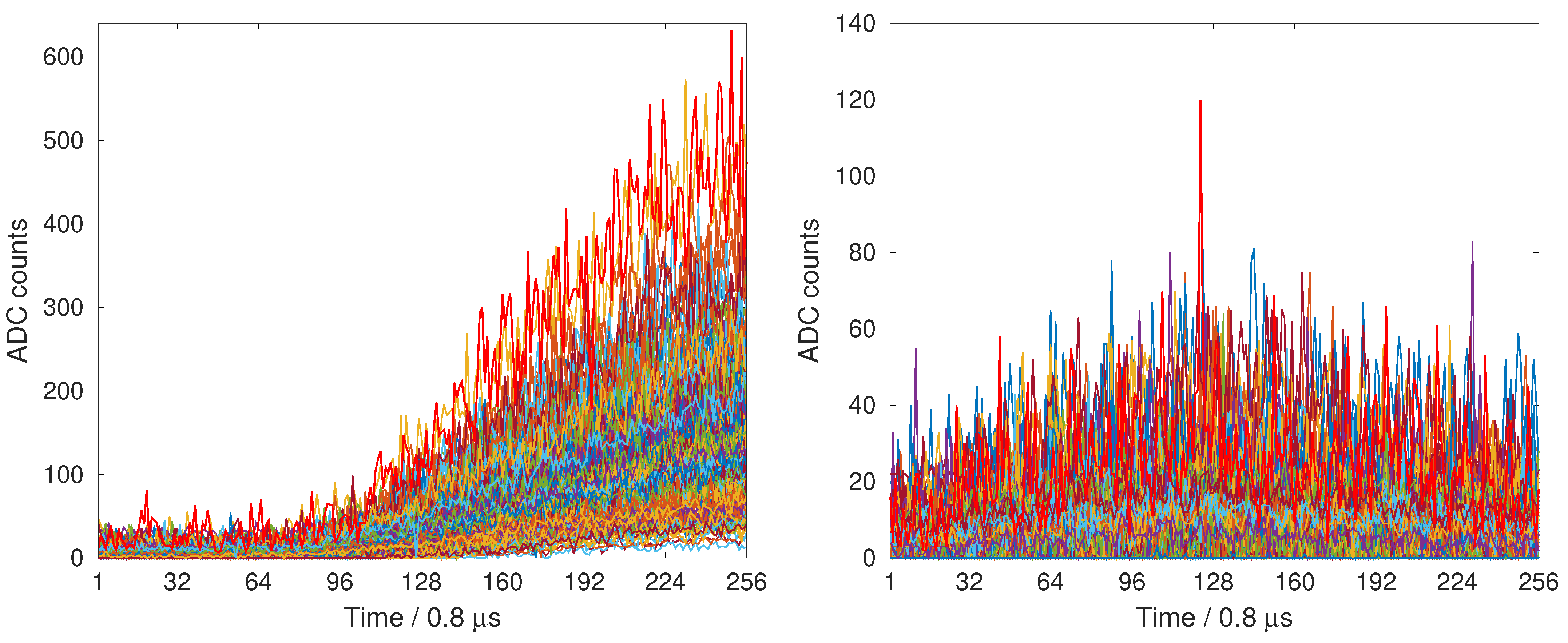
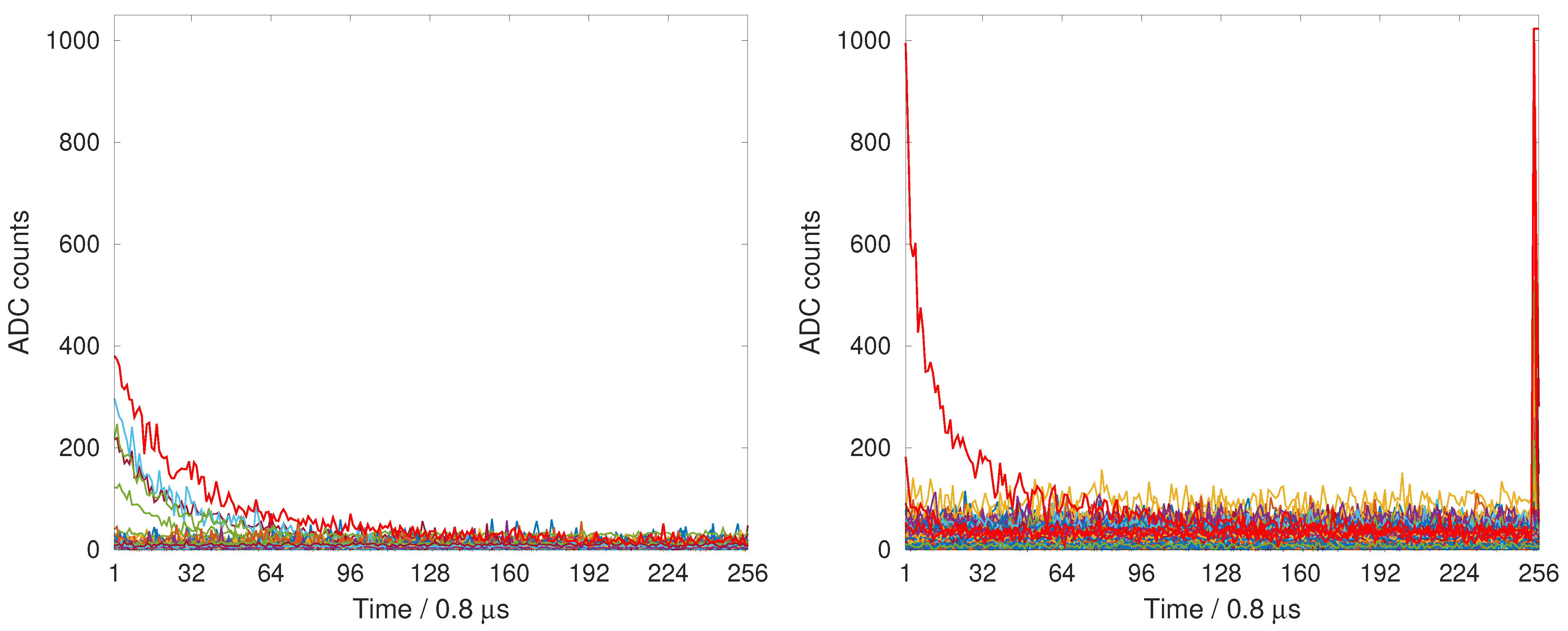
All slow flashes can be roughly divided into two groups: longer flashes that do not reach their maximum during a TUS record (see the left panel of Figure 7) and shorter flashes in which the signal passes its maximum and then attenuates, sometimes even reaching the level preceding the flash (see the right panel of Figure 7). Slow flashes of both groups differ in their amplitudes and the exact shape of waveforms but illumination of the focal surface is practically uniform in most cases up to sensitivity of channels. During this work, we have selected 113 slow flashes in which a rise of the signal was observed in at least 196 channels at ≥10 and calculated relative sensitivities of active channels assuming uniform illumination of the focal surface. The results qualitatively agreed with estimates obtained with a totally different technique presented in [33].
A comparison of geographic locations of slow flashes gave an immediate clue to their origin: they demonstrated a clear correlation with regions of high thunderstorm activity [12]. A set of then-known strong slow flashes registered from 16 August 2016, till 19 September 2016, was compared with the data on lightning strikes kindly provided by the World-Wide Lightning Location Network (WWLLN). It was found that there were “companion” lightnings within the time window s that corresponds to the accuracy of the TUS trigger for the majority of slow flashes. In most cases, the lightnings were registered at distances >400 km from the center of the field of view of TUS. It became clear that the likely origin of slow flashes with uniform illumination of the focal surface is light from distant lightning strikes that arrives at the mirror due to the lack of any side shields and becomes scattered.
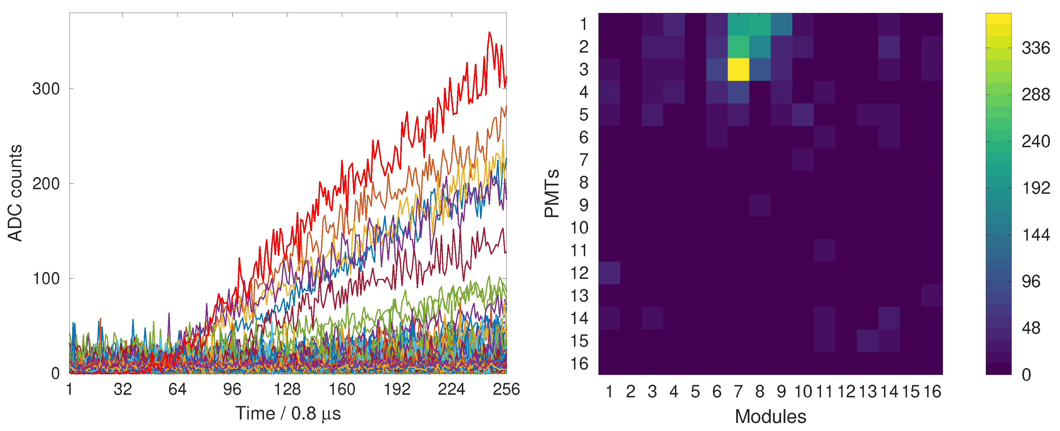
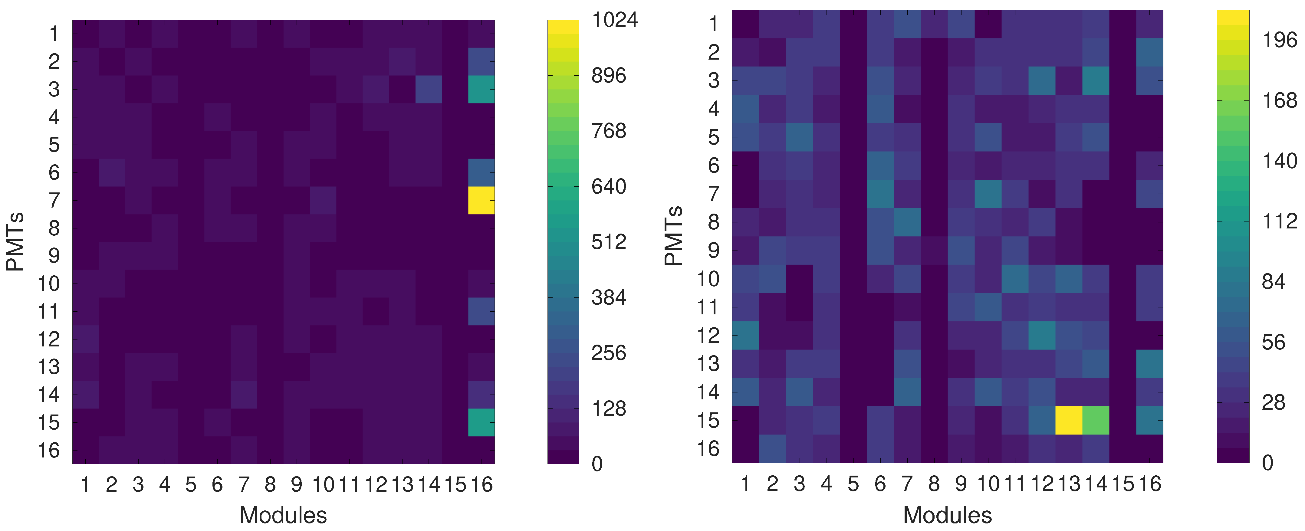
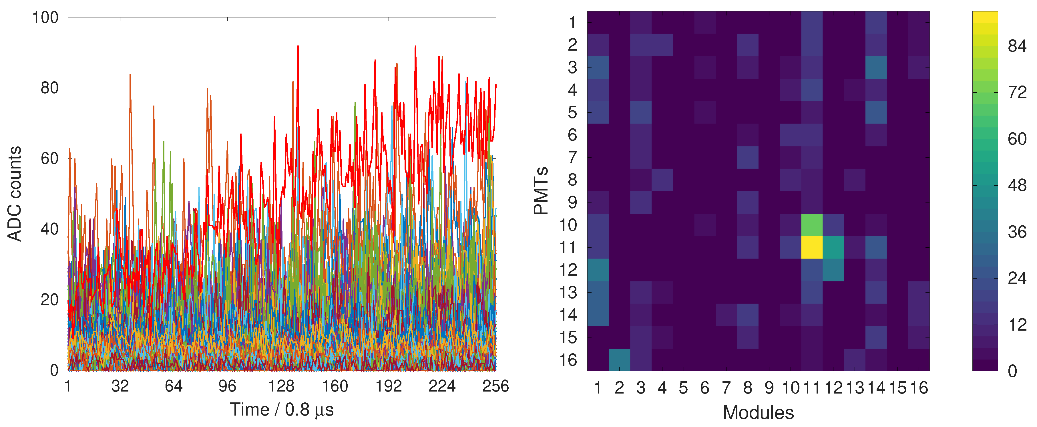
Illumination of the focal surface was found to be strongly non-uniform in some cases while waveforms were typical for slow flashes. An example is shown in Figure 8. In this particular case, two lightning strikes were registered by the Vaisala Global Lightning Dataset GLD360 [37,38] within s from the TUS trigger time stamp approximately at the position of the flash (within the FOV of TUS), see a bright spot in the right panel of Figure 8.
Slow flashes were occasionally registered simultaneously with other types of signals. The left panel of Figure 9 presents an example of a slow flash registered together with an instant track-like flash. The right panel of Figure 9 shows an ELVE evolving simultaneously with a slow flash. Interestingly, at least 15 out of 26 ELVEs found in the TUS data demonstrated a similar behavior.
4. Application of Neural Networks
There are multiple approaches to classification of data based on machine learning, see, e.g., [39]. Here we consider two simple architectures of neural networks. This is justified by two reasons. The first and most important one is that even these implementations demonstrate a very high accuracy of classification. Second, it is interesting to estimate if a neural network can be used onboard a satellite as a real-time trigger or anti-trigger for certain types of events. One should employ a simple neural network in this case since onboard processors have limited performance.
It is important to underline that TUS operated in different observational conditions that used to vary due to changes of the phase of the Moon, cloud coverage, humidity of the atmosphere, anthropogenic lights etc. A natural way to mitigate these factors would be to “flat-field” signals in different channels, i.e., to adjust ADC codes of all channels to a joint scale. Unfortunately, it is difficult to implement this accurately because, as mentioned above, 51 PMTs were totally damaged and sensitivities of the other channels changed after a malfunctioning of the high-voltage system during the first day of TUS operation. A few attempts for an in-flight calibration of the detector were performed but the estimates obtained are not accurate enough for a reliable adjustment of ADC codes in different channels to a joint scale. This complicates a classification of the TUS data within a uniform approach.
4.1. Instant Track-Like Flashes
As already mentioned in the introduction, results of the first application of neural networks to the analysis of the TUS data were briefly reported in [18]. Let us recall the main results of that study and discuss the subsequent analysis.
The main goal of [18] was to estimate if one can effectively employ neural networks as triggers or anti-triggers for certain types of signals that took place during the TUS mission and are likely to occur in the future orbital fluorescence telescopes aimed at studies of UHECRs. These should be simple neural networks since onboard processors have limited performance. The TLFs were chosen for the first study because, on the one hand, they have a simple structure but on the other hand they can hardly be avoided in orbital experiments.
Neural networks of two different architectures were considered. These were multilayer perceptrons (MLPs) and convolutional neural networks (CNNs). Perceptrons with 1, 2 and 3 hidden layers, consisting of 2–32 neurons were tested. To keep things simple, input data for perceptrons included only 512 numbers out of the whole set of 65,535 comprising a TUS event. The first 256 numbers contained ADC codes of a waveform with the highest amplitude and with the biggest FHDM in case there were several waveforms with the same amplitude. The second half of the input data represented a reshaped “snapshot” of the focal surface at the moment of the first maximum. The aim of these numbers was to separate TLFs from so-called “steep-front” events that had waveforms of the similar shape but used to illuminate the whole focal surface.
Results presented in [18] were mainly based on employing data of two months of observations with a subset of previously marked TLFs as a training data set. The data set included results of observations during October 2016, and April 2017. The choice was justified by a few considerations. October 2016, was approximately in the middle of the first period of regular observations in the EAS mode that lasted from 16 August till 16 December 2016. It contained 7888 events including 961 previously known TLFs. (Twenty-four other TLFs were found due to using NNs.) The second month contained data different from the first one in two respects. First, a preliminary version of an anti-trigger aimed to suppress TLFs was implemented in the onboard software of TUS in late March 2017. It did not work effectively enough but resulted in a shift of the moment of a signal rise in TUS records from time step around 60 to that around 30. This could influence the accuracy of neural networks. Second, another anti-trigger was uploaded to TUS on 28 April 2017. This anti-trigger effectively suppressed the majority of TLFs but left space for “tails” of the most long-lasting of them, see an example below. Such events were necessary for a proper training of the NNs. The set recorded in April, 2017, consisted of 8103 events, including 370 TLFs. We tried several other ways of selecting training data sets within the present work, including random sampling, but they did not demonstrate any considerable benefits in comparison with the initial choice.
The main part of the analysis presented in [18] employed MLPs with two hidden layers with 8 neurons in each of them. The TLFs were selected in advance with a conventional algorithm that looked for an instant growth of the signal over the background by more than 20 . Such perceptrons demonstrated an accuracy ≥0.995 on the training data but the accuracy of even more simple neural networks was not drastically lower. The accuracy of classification on the test data sample was also pretty high: the networks used to make ∼200 wrong predictions in the data set of more than 61 thousand events. Most mistakes related to low-amplitude flashes confined to a single pixel with a comparatively high level of the background signal similar to the one shown in the right panel of Figure 2. This kind of signals was also the most difficult one for the conventional algorithm.
We also tested several configurations of CNNs. The network used in [18] consisted of a convolutional layer with 20 filters and a kernel, a maximum pooling layer, a hidden dense layer with 64 neurons and an output layer. In the subsequent analysis reported below, the CNN was complemented with a dropout layer and a dense hidden layer with 256 neurons going after the pooling layer. The output layer used sigmoid as an activation function; the other layers used ReLU. The Adam algorithm was used as an optimizer. A procedure for an early stop of training to prevent an overfitting of the neural network and an adjustable learning rate available in Keras were employed.
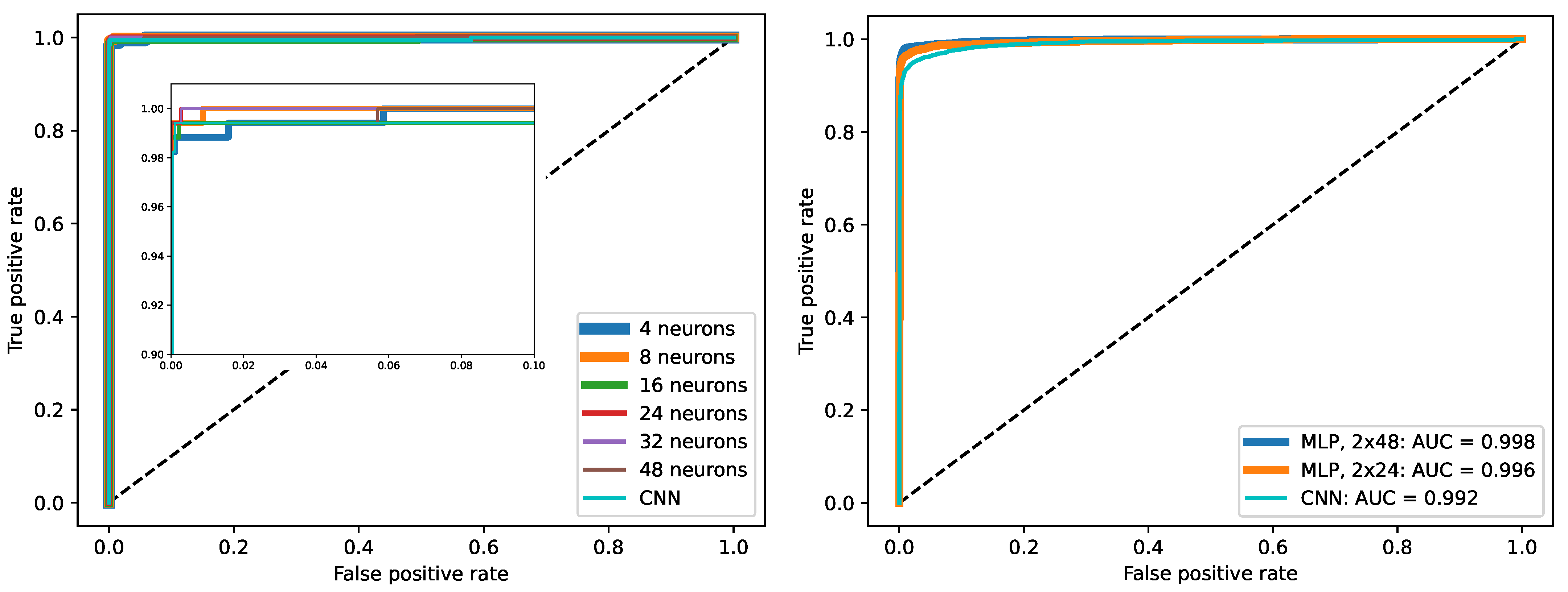
The highest accuracy of the CNN was obtained with every event in the input sample represented by 768 numbers. These were “snapshots” of the focal surface made at the first moment of an event, at the moment of the first maximum of ADC codes and at the last moment. These snapshots were arranged in three layers so that the signal in each pixel was described by three numbers similar to RGB images. Table 1 provides some numbers that illustrate the training stage of the CNN and several MLPs with two hidden layers but different number of nodes in each of them (from 4 to 48). The sample consisted of nearly 16,000 events, 2000 of which were used for testing the trained networks. Twenty percent of the rest of the sample were employed as a validating sample. Neural networks of each configuration were trained ten times with different initial weights. It can be seen that performance of MLPs was very high in all cases and only slightly depended on the number of neurons in the hidden layers. The CNN demonstrated higher accuracy than MLPs during training but its testing accuracy was slightly lower than for MLPs with more than 24 neurons in each hidden layer. We do not include data for perceptrons with more hidden layers or neurons because we did not find an increase of accuracy with such networks.
Figure 10 presents ROC (Receiver Operating Characteristic) curves that illustrate the efficiency of different architectures of neural networks employed in searching for TLFs. The left panel shows ROC curves for the training stage of the CNN and 2-layer MLPs with 4, 8, ..., 48 neurons in each hidden layer. It is clearly seen that there is very little difference in performance of MLPs with ≥8 nodes and the CNN. The right panel shows ROC curves for the testing stage of the CNN and 2-layer MLPs with 24 and 48 nodes in each layer. In this case the MLPs performed slightly better than the CNN with the area under the curve (AUC) equal to 0.996 and 0.998 respectively in comparison with 0.992 for the CNN. A reason MLPs slightly outperformed the CNN might be the specific type of waveforms in track-like flashes that can be easily recognized by an MLP (in most cases) and a much more rich variety of their traces on the focal surface, partially due to dead or buggy pixels and some glitches of the electronics discussed above.
A few examples of snapshots of the focal surface of TLFs that were not properly classified by the CNN are shown in Figure 11. On the other hand, there were several events that were mistakenly classified as TLFs by the CNN. Two examples of such false positives are presented in Figure 12. It is immediately apparent from the waveforms that the events were not track-like flashes but the snapshots were confusing for the neural network. Events with tracks similar to those shown in Figure 6 also posed a problem for the CNN. It is unlikely that issues such as these will take place with orbital fluorescence telescopes with higher spatial resolution, smaller pixels and other electronics systems.
Neither of the two false positives shown in Figure 12 (nor similar ones) posed a problem for the MLPs. However, the CNN was more effective when detecting “tails” of TLFs that used to occur from time to time in the data after the majority of TLFs were suppressed by the anti-trigger, see the left panel in Figure 13 for an example of such event. More than this, the CNN trained on data represented by 768 numbers in the way described above was able to classify properly TLFs such as the one shown in the right panel of Figure 13. Such events used to appear in the period from May till August 2016 due to a bug in the onboard software that resulted in an incorrect sequence of ADC codes, putting the first moment of time somewhere around the middle of the record.
Interestingly, neither increasing the amount of data used for a description of every TUS event, nor a few modifications of the CNN lead to an improvement of the accuracy of classification. Even CNNs employing all available ADC codes in events used for training demonstrated lower accuracy on the testing sample than the CNN employing 768 numbers. They were sometimes confused by events in which the peak of the signal was located close to the beginning or to the end of the record. This might be because the moment of the instant growth of the signal was not always the same in the TUS data. On the one hand, CNNs that employed complete records for training resulted in classifying very weak signals on a strong background as TLFs which we were unable to verify as being such.
Remarkably, the neural networks found more than 400 weak TLFs not identified as such by the conventional algorithm. This increased the number of TLFs found in the TUS data by approximately 10% resulting in nearly 4000 events in the whole TUS data set. (Obviously, one could lower the threshold of the signal jump in the conventional algorithm but this used to lead to a high number of false positives caused by kinks that were likely to be just random fluctuations of the signal).
One can notice that the training data set used in [18] was strongly imbalanced with TLFs comprising only around 8.5% of the whole training sample. It is known that using imbalanced data can lead to a sub-optimal accuracy of a neural network. We studied this issue by creating random samples of data used for training instead of using continuous periods of time, with TLFs representing from 20% to 50% of the whole samples. We did not find any significant improvement of the accuracy of NNs trained on these samples when applied to testing data. More than this, in some cases this resulted in a growth of the number of false positives.
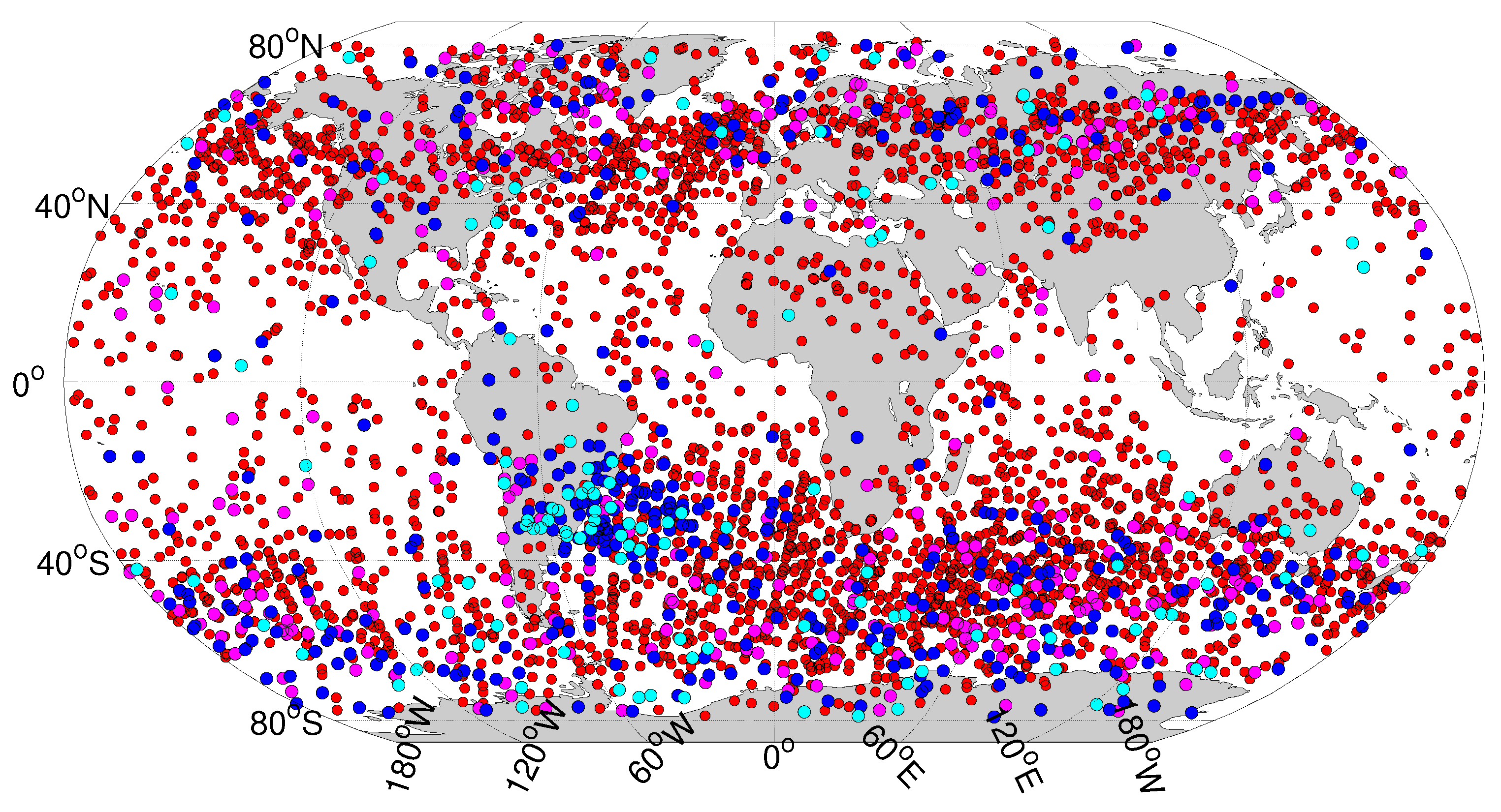
Geographical locations of instant track-like flashes in the final sample are shown in Figure 14. It is clearly seen that the majority of TLFs had high amplitudes. In fact, 2787 of them had amplitudes equal to 1023 ADC counts thus saturating PMTs. Only 131 TLFs in the sample had amplitudes ≤200. Most of them were found in the region of the South-Atlantic anomaly, a huge area in the Southern hemisphere, where the inner Van Allen radiation belt comes closest to the Earth’s surface, going down to an altitude of around 200 km, which leads to an increased flux of energetic particles in this region1.
4.2. Slow Flashes
Every TUS event can be considered to be a video consisting of 256 frames with a resolution of each. One of the established approaches for classification of videos is using so-called convolutional long short-term memory neural networks, see, e.g., [40]. However, we found them more demanding on computational resources than the CNN considered here or its slight modifications without any noticeable benefit in terms of accuracy. Thus, in what follows, we only consider an application of the CNN described above with different ways of arranging input data.
It was clear from the very beginning that snapshots of TUS records made at the first and last time steps and at the moment of the signal maximum will be insufficient for an effective representation of slow flashes because they do not have a characteristic instant “jump” of the signal as TLFs. We tried several ways of preparing input data, mainly by using samples uniformly distributed within a record. We tested input data represented as 4, 8, 16, 32, 64, 128 and 256 snapshots of the focal surface arranged in a stack (a “sandwich”) with the respective number of layers. None of the different ways of arranging input data demonstrated significant benefits over the other in terms of the accuracy. In a typical run, the best testing accuracy was approximately equal to 0.999, the best validation accuracy was of the order of 0.99, and the testing accuracy varied in the range 0.980–0.988. However, the time needed for training used to grow considerably with an increasing number of layers. We have chosen 16 snapshots of the focal surface uniformly distributed within a record as the main way of representing input data. Thus, only 4096 numbers (ADC codes) of the total 65,536 were used to represent each of the TUS events.
We used different samples for training the network. In what follows, we discuss results obtained by employing a sample of 16 thousand events registered during October 2016, and July 2017. One thousand events acted as a testing sample, others were used for training with 20% of them forming a validation set.
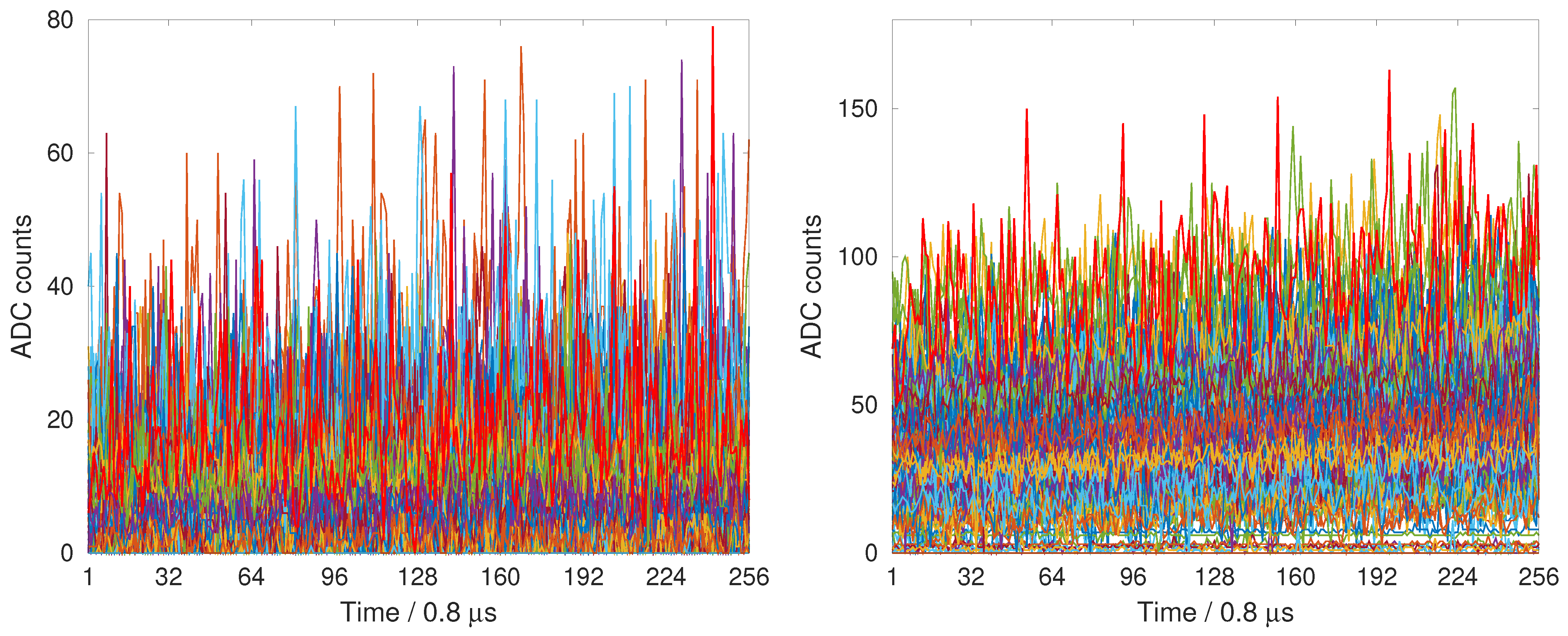
The process of training the CNN brought several surprises. Initially, the training sample included 798 slow flashes selected by a conventional algorithm. Training the network resulted in a considerable number of “false positives” that either had low amplitudes without obvious signs of a “collective” behavior similar to that shown in Figure 7, or were registered on a strong background, mostly during periods around a full Moon. A closer inspection of these events revealed that they could possibly be slow flashes. A couple of examples of such events is presented in Figure 15.
At this stage, we focused on a data set registered from 16 August 2016, till 19 September 2017, since we had the WWLLN data for it. The initial sample of slow flashes for this period consisted of 175 events (out of 6584 events in the whole sample). An analysis of all “false positives” selected by the CNN revealed a correlation between all new events selected around the full Moon and 76 out of 78 weak events on the one hand and companion lightnings/thunderstorms on the other hand. In particular, 5 strikes were registered by the WWLLN in less than 1 s after the event shown in the left panel of Figure 15 in 440–470 km from the center of the FOV of TUS. Another strong thunderstorm was taking place at the moment of registering an event shown in the right panel of Figure 15 with 6 lightnings registered within 1 s from the TUS trigger time stamp at distances around 680 km. This could not unequivocally prove that these events were due to distant lightning strikes but provided evidence that the CNN might be more sensitive to weak slow flashes than the “traditional” algorithm and that at least a part of events selected as “false positives” could be slow flashes.
Since we did not have data on lightning strikes for the rest of the TUS data, we looked for another conventional tool that could help in judging if an event newly selected by the CNN could be a slow flash. We have found that waveforms of almost all slow flashes (except the most violent ones that resulted in a saturation of the focal surface) could be nicely smoothed with a Hamming window of size 128 and fitted with a Gaussian, and the number of good fits was ≥10. Similar to correlations with lightnings, this test could not prove that a particular event was or was not a slow flash in terms of its origin related to lightning strikes. However, we employed it in later studies to be on the conservative side when checking doubtful events selected by the CNN.
To deal with the incompletely marked training data set, we applied the following iterative procedure. After training the CNN, we visually checked all new “false positives” and in the case of doubts applied the above mentioned “smooth-and-fit” procedure to them. Then we repeated training with a new list of slow flashes, and performed a similar check. The cycle was continued until the number of “false positives” reduced to just a few events. This way, the list of slow flashes for October 2016, and July 2017, increased from the initial 798 to 1805 events. The CNN was trained then with this final list of slow flashes and applied to the rest of the data resulting in a sample of nearly 8300 events in comparison with the initial 3327.
All newly selected events were checked and more than 100 of them were excluded from the final sample. More than 30 of them were events with a weak signal and very few or zero good fits of the waveforms. Eighteen excluded events represented so-called “steep-front flashes” mentioned above that are similar to slow flashes in that they mostly illuminate the whole focal surface but have waveforms close to TLFs. The instant growth of the signal in this type of events could not be identified with input data using only 16 uniformly distributed slices of the whole record. A few events registered on the terminator with low values of the high-voltage system were excluded, too. Finally, a few excluded events looked similar to the event with a non-uniform illumination of the focal surface shown in Figure 8. One of these events is shown in Figure 16. It was registered on 3 November 2016, above North Canada. We did not find any information on lightning strikes or thunderstorms in the region on that date but found that the field of view of active channels coincides with the location of a small settlement called Igloolik. The place appears as a small bright spot on the surrounding dark background in DMSP-OLS Nighttime Lights maps obtained in the visible and infrared range2. Since all events of this kind were registered above populated areas, we conclude they are likely to have an anthropogenic origin.
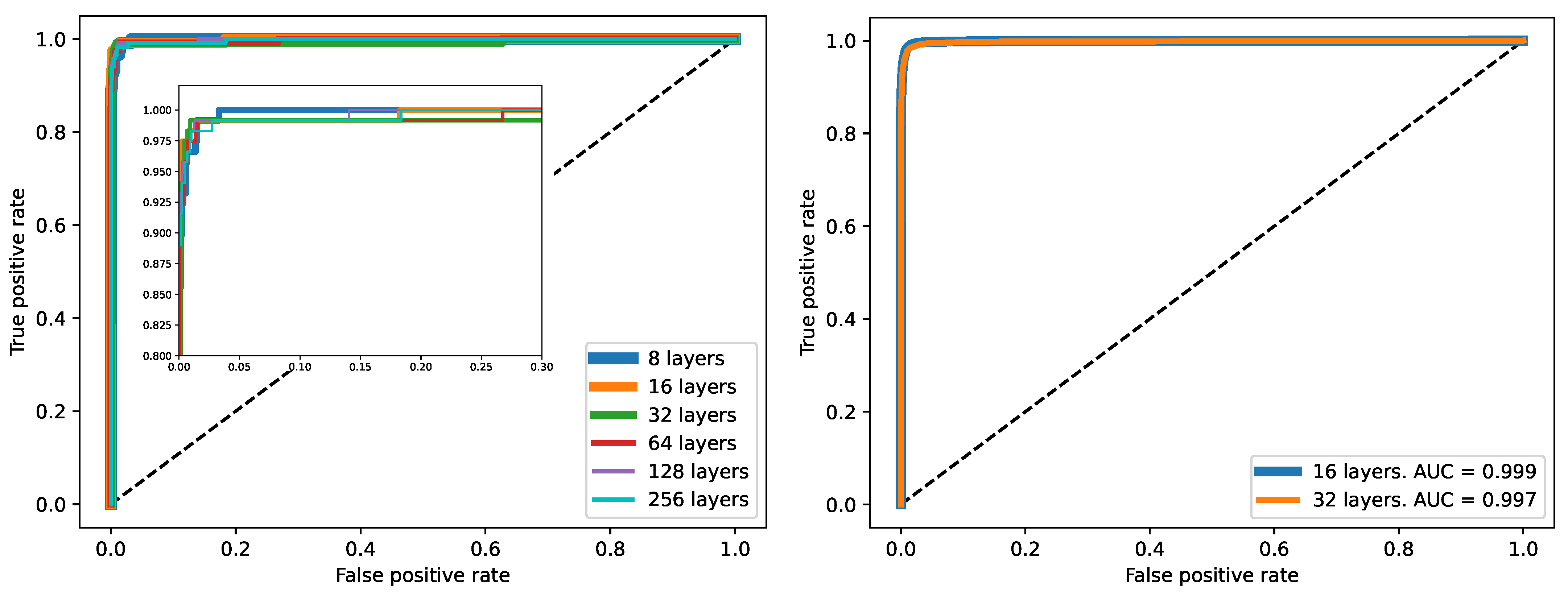
In the end, we obtained a set of more than 8100 events classified by the CNN as slow flashes, which was approximately 2.4 times larger than the initial sample selected with the conventional algorithm. At this moment we repeated an analysis of performance of CNNs using different arrangement of the input data to verify if the initial choice of the 16-layer representation was correct. The left panel of Figure 17 shows ROC curves for the training stage of CNNs that employed input data arranged in 8, 16, 32, 64, 128 and 256 layers sampled uniformly from complete records. It can be seen that CNNs trained with 8- and 256-layer samples performed slightly worse than the others but the difference was negligible. The right panel shows ROC curves for the testing stage of the CNNs that used 16- and 32-layer input samples. The CNN that used simpler data representation (16 layers) performed marginally better than the CNN with 32-layer data (AUC was equal to 0.999 vs. 0.997 respectively).
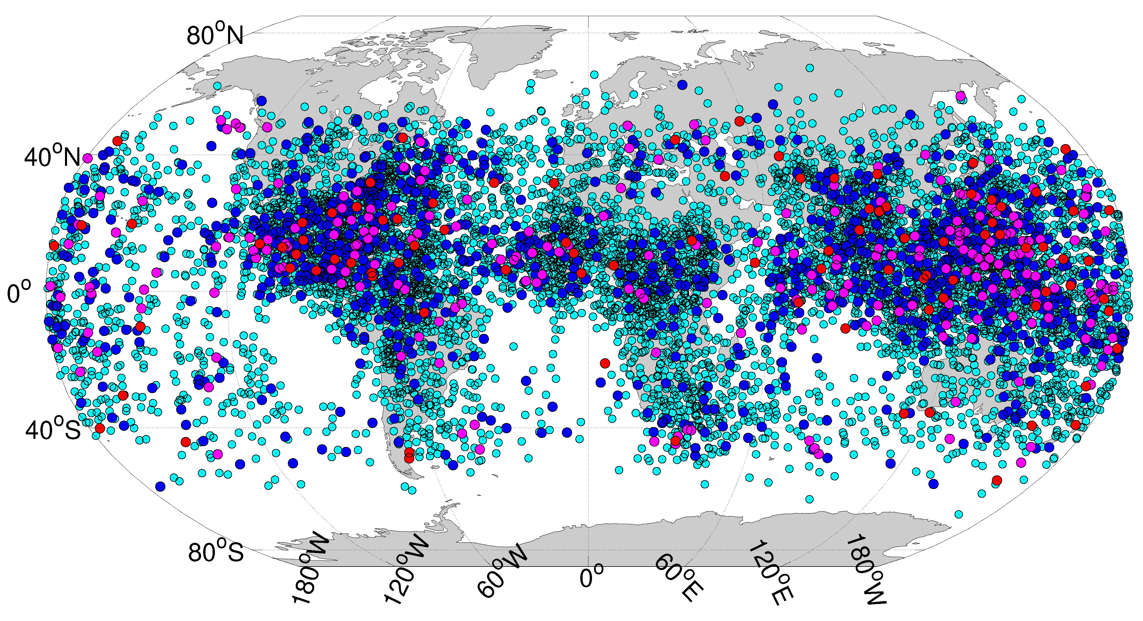
Geographical locations of slow flashes in the final sample are shown in Figure 18. It is clearly seen that they form three huge spots around the main regions of high thunderstorm activity around the Caribbean, central Africa and South-East Asia. Noticeably, the distribution of amplitudes of slow flashes is in a sense opposite to that of TLFs with weak flashes forming the majority of the sample.
Similar to the case of classifying track-like flashes, the training sets were imbalanced: slow flashes made up ∼10% of the samples. However, a rearrangement of data demonstrated that this did not lead to a decrease in the accuracy of training.
5. Discussion
We presented results of using two types of neural networks—multilayer perceptrons and convolutional networks—for classification of data obtained with the TUS orbital fluorescence telescope. The architecture of the neural networks was simple and did not put high demands on computer facilities so that all calculations presented in the work were performed on a desktop PC without a GPU. Nevertheless, both MLPs and CNNs demonstrated a high accuracy in classifying two types of events registered by TUS: instant track-like flashes produced by cosmic ray hits of the focal surface of the detector and so-called slow flashes that used to originate from distant lightnings. More than this, the application of neural networks allowed us to increase the number of previously known TLFs by approximately 20% and the number of slow flashes by 2.4 times due to the discovery of weak signals omitted by conventional algorithms.
To overcome the incompleteness of marks in the training data sets, we performed an iterative procedure in which all events selected as false positives after a run were thoroughly checked and marked as representatives of the respective class if necessary. The cycle was repeated until there were no doubts left that the overwhelming majority of events in the data set were divided into classes properly. We employed data from the World-Wide Lightning Location Network for a certain period of observations to verify the validity of classifying slow flashes by the neural network. However, it is necessary to note that the final samples could contain several erroneous records due to the incompleteness of data on lightning strikes and the fuzzy nature of weak signals in the TUS data.
The latter is worth a special comment. We have already mentioned that we faced certain problems when trying to classify weak signals, be it slow flashes or track-like flashes: a visual analysis of some weak signals did not give a clear clue on how to classify them. In the case of TLFs, one has no way to verify if a weak kink in ADC codes was caused by a low-energy charged particle hitting a single PMT or it was just a random fluctuation of the signal. The only way to check this to some extent is to perform more detailed simulations of the photodetector. The situation with slow flashes seems more complicated in this respect. In principle, one can add information on lightnings to the classifier. However, to the best of the author’s knowledge, there is currently no network of lightning detectors uniformly covering the Earth. Even in case there was one, it would be difficult to judge unequivocally if a particular lightning resulted in a slow flash registered by TUS because of the low accuracy of its timestamps in comparison with those for lightnings, a wide variety of energies of lightnings and the diversity of their types. One might expect that intra-cloud, cloud-to cloud and cloud-to-ground lightnings of the same power used to produce different illumination of the TUS mirror. A detailed simulation seems to be needed to better understand the phenomenon. However, the approach looks promising if applied to lightnings within the FOV of a telescope that has more precise timestamps.
It was interesting to find out that different architectures of neural networks and different representations of input data might be needed for classification of different types of signals within the same data set. It was also remarkable that there was no need to use complete records of events for their effective classification. More than this, networks trained on especially crafted subsets of complete records demonstrated higher classification accuracy than those employing full data.
We believe that our results help to better understand the data obtained during the TUS mission. This is important because the TUS data set provides significant information about the processes taking place in the nocturnal atmosphere of the Earth in the UV band, which comprise the background for registering UHECRs by the future full-scale orbital experiments. A proper classification of these signals, including weak ones, will help to reduce the background and possibly to develop triggers finely tuned for registering UHECRs and suppressing “parasitic” signals. In the case of TUS, effective anti-triggers for slow flashes and instant track-like events could have increased the amount of “useful” data by more than 15%. This can strongly improve the efficiency of orbital missions, especially taking into account their limited hardware and telemetry budgets. We plan to apply the experience obtained during the present study for classification of data of the Mini-EUSO detector currently operating at the ISS and for the fluorescence telescopes that are under development.
Let us finally remark that there is another type of machine learning methods that is widely used for classification of data but is very different from the approach used in the paper. This is the decision tree and its multiple variants (gradient boosted trees, random forest etc.). They are in particular famous because of the simplicity of understanding and interpreting their results. We are going to employ this approach and compare it to the presented results in another paper.
Funding
The research was supported by the Interdisciplinary Scientific and Educational School of Lomonosov Moscow State University “Fundamental and Applied Space Research”.
Data Availability Statement
The TUS data is available upon agreement with Lomonosov Moscow State University.
Acknowledgments
I thank Margarita Kaznacheeva for the initial data set of slow flashes and a helpful discussion.
Conflicts of Interest
The authors declare no conflict of interest.
| 1 | https://heasarc.gsfc.nasa.gov/docs/rosat/gallery/misc_saad.html, accessed on 22 June 2021. |
| 2 | https://ngdc.noaa.gov/eog/dmsp/downloadV4composites.html, accessed on 31 May 2021. |
References
- Baltrusaitis, R.M.; Cady, R.; Cassiday, G.L.; Cooperv, R.; Elbert, J.W.; Gerhardy, P.R.; Ko, S.; Loh, E.C.; Salamon, M.; Steck, D.; et al. The Utah Fly’s Eye detector. Nucl. Instrum. Methods Phys. Res. A 1985, 240, 410–428. [Google Scholar] [CrossRef]
- Abraham, J.; Abreu, P.; Aglietta, M.; Aguirre, C.; Ahn, E.J.; Allard, D.; Allekotte, I.; Allen, J.; Allison, P.; Alvarez-Muñiz, J.; et al. The fluorescence detector of the Pierre Auger Observatory. Nucl. Instrum. Methods Phys. Res. Sect. A Accel. Spectrom. Detect. Assoc. Equip. 2010, 620, 227–251. [Google Scholar] [CrossRef] [Green Version]
- Tokuno, H.; Tameda, Y.; Takeda, M.; Kadota, K.; Ikeda, D.; Chikawa, M.; Fujii, T.; Fukushima, M.; Honda, K.; Inoue, N.; et al. New air fluorescence detectors employed in the Telescope Array experiment. Nucl. Instrum. Methods Phys. Res. Sect. Accel. Spectrom. Detect. Assoc. Equip. 2012, 676, 54–65. [Google Scholar] [CrossRef] [Green Version]
- Greisen, K. End to the cosmic-ray spectrum? Phys. Rev. Lett. 1966, 16, 748–750. [Google Scholar] [CrossRef]
- Zatsepin, G.T.; Kuz’min, V.A. Upper limit of the spectrum of cosmic rays. Sov. J. Exp. Theor. Phys. Lett. 1966, 4, 78. [Google Scholar]
- Benson, R.; Linsley, J. Satellite observation of cosmic-ray air showers. Bull. Am. Astron. Soc. 1980, 12, 818. [Google Scholar]
- Benson, R.; Linsley, J. Satellite observation of cosmic ray air showers. In Proceedings of the 17th International Cosmic Ray Conference, Paris, France, 13–25 July 1981; Volume 8, pp. 145–148. [Google Scholar]
- Ormes, J.F.; Barbier, L.M.; Boyce, K.; Christian, E.; Krizmanic, J.F.; Mitchell, J.F.; Stecker, F.; Stilwell, D.E.; Streitmatter, R.E.; Chipman, R.A.; et al. Orbiting wide-angle light collectors (OWL): A pair of earth orbiting “eyes” to study air showers initiated by >1020 eV particles. In Proceedings of the International Cosmic Ray Conference, Durban, South Africa, 28 July–8 August 1997; Volume 5, p. 273. [Google Scholar]
- Khrenov, B.A.; Panasyuk, M.I.; Alexandrov, V.V.; Bugrov, D.I.; Cordero, A.; Garipov, G.K.; Linsley, J.; Martinez, O.; Salazar, H.; Saprykin, O.A.; et al. Space program KOSMOTEPETL (project KLYPVE and TUS) for the study of extremely high energy cosmic rays. In Observing Ultrahigh Energy Cosmic Rays from Space and Earth, Proceedings of the AIP Conference Proceedings 566, Metepec, Mexico, 9–12 August 2000; American Institute of Physics Conference Series; Salazar, H., Villasenor, L., Zepeda, A., Eds.; American Institute of Physics: College Park, MD, USA, 2001; Volume 566, pp. 57–75. [Google Scholar]
- Alexandrov, V.V.; Bugrov, D.I.; Garipov, G.K.; Grebenyuk, V.M.; Finger, M.; Khrenov, B.A.; Linsley, J.; Martinez, O.; Panasyuk, M.I.; Salazar, H.; et al. Space experiment TUS for study of ultra high energy cosmic rays. In Proceedings of the International Cosmic Ray Conference, Hamburg, Germany, 7–15 August 2001; Volume 2, p. 831. [Google Scholar]
- Adams, J.H.; Ahmad, S.; Albert, J.N.; Allard, D.; Anchordoqui, L.; Andreev, V.; Anzalone, A.; Arai, Y.; Asano, K.; Pernas, M.; et al. The JEM-EUSO mission: An introduction. Exp. Astron. 2015, 40, 3–17. [Google Scholar] [CrossRef] [Green Version]
- Khrenov, B.A.; Klimov, P.A.; Panasyuk, M.I.; Sharakin, S.A.; Tkachev, L.G.; Zotov, M.Y.; Biktemerova, S.V.; Botvinko, A.A.; Chirskaya, N.P.; Eremeev, V.E.; et al. First results from the TUS orbital detector in the extensive air shower mode. J. Cosmol. Astropart. Phys. 2017, 9, 006. [Google Scholar] [CrossRef] [Green Version]
- Zotov, M. Early results from TUS, the first orbital detector of extreme energy cosmic rays. In Proceedings of the Ultra-High Energy Cosmic Rays (UHECR2016), Kyoto, Japan, 11–14 October 2016; p. 011029. [Google Scholar]
- Bertaina, M.; Castellina, A.; Cremonini, R.; Fenu, F.; Klimov, P.; Salsi, A.; Sharakin, S.; Shinozaki, K.; Zotov, M. Search for extreme energy cosmic rays with the TUS orbital telescope and comparison with ESAF. Eur. Phys. J. Web Conf. 2019, 210, 06006. [Google Scholar] [CrossRef] [Green Version]
- Klimov, P.; Khrenov, B.; Kaznacheeva, M.; Garipov, G.; Panasyuk, M.; Petrov, V.; Sharakin, S.; Shirokov, A.; Yashin, I.; Zotov, M.; et al. Remote sensing of the atmosphere by the ultraviolet detector TUS onboard the Lomonosov satellite. Remote Sens. 2019, 11, 2449. [Google Scholar] [CrossRef] [Green Version]
- Khrenov, B.A.; Garipov, G.K.; Kaznacheeva, M.A.; Klimov, P.A.; Panasyuk, M.I.; Petrov, V.L.; Sharakin, S.A.; Shirokov, A.V.; Yashin, I.V.; Zotov, M.Y.; et al. An extensive-air-shower-like event registered with the TUS orbital detector. J. Cosmol. Astropart. Phys. 2020, 2020, 033. [Google Scholar] [CrossRef] [Green Version]
- Khrenov, B.A.; Garipov, G.K.; Zotov, M.Y.; Klimov, P.A.; Panasyuk, M.I.; Petrov, V.L.; Sharakin, S.A.; Shirokov, A.V.; Yashin, I.V.; Grebenyuk, V.M.; et al. A study of atmospheric radiation flashes in the near-ultraviolet region using the TUS detector aboard the Lomonosov satellite. Cosm. Res. 2020, 58, 317–329. [Google Scholar] [CrossRef]
- Zotov, M.Y.; Sokolinskiy, D.B. The first application of neural networks to the analysis of the TUS orbital detector data. Mosc. Univ. Phys. Bull. 2020, 75, 657–664. [Google Scholar] [CrossRef]
- Erdmann, M.; Glombitza, J.; Walz, D. A deep learning-based reconstruction of cosmic ray-induced air showers. Astropart. Phys. 2018, 97, 46–53. [Google Scholar] [CrossRef]
- Guillén, A.; Bueno, A.; Carceller, J.M.; Martínez-Velázquez, J.C.; Rubio, G.; Peixoto, C.J.; Sanchez-Lucas, P. Deep learning techniques applied to the physics of extensive air showers. Astropart. Phys. 2019, 111, 12–22. [Google Scholar] [CrossRef] [Green Version]
- Vrábel, M.; Genci, J.; Bobik, P.; Bisconti, F. Machine learning approach for air shower recognition in EUSO-SPB data. In Proceedings of the 36th International Cosmic Ray Conference (ICRC2019), Madison, WI, USA, 24 July–1 August 2019; Volume 36, p. 456. [Google Scholar]
- Kalashev, O. Using deep learning in ultra-high energy cosmic ray experiments. J. Phys. Conf. Ser. 2020, 1525, 012001. [Google Scholar] [CrossRef]
- Ivanov, D.; Kalashev, O.E.; Kuznetsov, M.Y.; Rubtsov, G.I.; Sako, T.; Tsunesada, Y.; Zhezher, Y.V. Using deep learning to enhance event geometry reconstruction for the Telescope Array surface detector. arXiv 2020, arXiv:2005.07117. [Google Scholar] [CrossRef]
- Spencer, S.; Armstrong, T.; Watson, J.; Mangano, S.; Renier, Y.; Cotter, G. Deep learning with photosensor timing information as a background rejection method for the Cherenkov Telescope Array. Astropart. Phys. 2021, 129, 102579. [Google Scholar] [CrossRef]
- The Pierre Auger Collaboration. Deep-learning based reconstruction of the shower maximum Xmax using the water-cherenkov detectors of the Pierre Auger Observatory. arXiv 2021, arXiv:2101.02946. [Google Scholar]
- Erdmann, M.; Glombitza, J. Deep learning based algorithms in astroparticle physics. J. Phys. Conf. Ser. 2020, 1525, 012112. [Google Scholar] [CrossRef]
- Bacholle, S.; Barrillon, P.; Battisti, M.; Belov, A.; Bertaina, M.; Bisconti, F.; Blaksley, C.; Blin-Bondil, S.; Cafagna, F.; Cambiè, G.; et al. Mini-EUSO mission to study earth UV emissions on board the ISS. Astrophys. J. Suppl. Ser. 2021, 253, 36. [Google Scholar] [CrossRef]
- Adams, J.H., Jr.; Anchordoqui, L.A.; Apple, J.A.; Bertaina, M.E.; Christl, M.J.; Fenu, F.; Kuznetsov, E.; Neronov, A.; Olinto, A.V.; Parizot, E.; et al. White paper on EUSO-SPB2. arXiv 2017, arXiv:1703.04513. [Google Scholar]
- Olinto, A.V.; Krizmanic, J.; Adams, J.H.; Aloisio, R.; Anchordoqui, L.A.; Anzalone, A.; Bagheri, M.; Barghini, D.; Battisti, M.; Bergman, D.R.; et al. The POEMMA (Probe of Extreme Multi-Messenger Astrophysics) observatory. arXiv 2020, arXiv:2012.07945. [Google Scholar]
- Chollet, F.; et al. Keras. 2015. Available online: https://keras.io (accessed on 31 May 2021).
- Abadi, M.; Agarwal, A.; Barham, P.; Brevdo, E.; Chen, Z.; Citro, C.; Corrado, G.S.; Davis, A.; Dean, J.; Devin, M.; et al. TensorFlow: Large-Scale Machine Learning on Heterogeneous Systems. 2015. Available online: https://tensorflow.org (accessed on 31 May 2021).
- Klimov, P.A.; Panasyuk, M.I.; Khrenov, B.A.; Garipov, G.K.; Kalmykov, N.N.; Petrov, V.L.; Sharakin, S.A.; Shirokov, A.V.; Yashin, I.V.; Zotov, M.Y.; et al. The TUS detector of extreme energy cosmic rays on board the Lomonosov satellite. Space Sci. Rev. 2017, 212, 1687–1703. [Google Scholar] [CrossRef]
- Klimov, P.A.; Sigaeva, K.F.; Sharakin, S.A. Flight calibration of the photodetector in the TUS detector. Instrum. Exp. Tech. 2021, 64, 450–455. [Google Scholar] [CrossRef]
- Fukunishi, H.; Takahashi, Y.; Kubota, M.; Sakanoi, K.; Inan, U.S.; Lyons, W.A. Elves: Lightning-induced transient luminous events in the lower ionosphere. Geophys. Res. Lett. 1996, 23, 2157–2160. [Google Scholar] [CrossRef]
- Allison, J.; Amako, K.; Apostolakis, J.; Arce, P.; Asai, M.; Aso, T.; Bagli, E.; Bagulya, A.; Banerjee, S.; Barrand, G.; et al. Recent developments in GEANT4. Nucl. Instrum. Methods Phys. Res. A 2016, 835, 186–225. [Google Scholar] [CrossRef]
- Klimov, P.A.; Zotov, M.Y.; Chirskaya, N.P.; Khrenov, B.A.; Garipov, G.K.; Panasyuk, M.I.; Sharakin, S.A.; Shirokov, A.V.; Yashin, I.V.; Grinyuk, A.A.; et al. Preliminary results from the TUS ultra-high energy cosmic ray orbital telescope: Registration of low-energy particles passing through the photodetector. Bull. Russ. Acad. Sci. Phys. 2017, 81, 407–409. [Google Scholar] [CrossRef]
- Said, R.K.; Inan, U.S.; Cummins, K.L. Long-range lightning geolocation using a VLF radio atmospheric waveform bank. J. Geophys. Res. Atmos. 2010, 115, D23108. [Google Scholar] [CrossRef] [Green Version]
- Said, R.K.; Cohen, M.B.; Inan, U.S. Highly intense lightning over the oceans: Estimated peak currents from global GLD360 observations. J. Geophys. Res. Atmos. 2013, 118, 6905–6915. [Google Scholar] [CrossRef] [Green Version]
- Goodfellow, I.; Bengio, Y.; Courville, A. Deep Learning; MIT Press: Cambridge, MA, USA, 2016; Available online: http://www.deeplearningbook.org (accessed on 31 May 2021).
- Donahue, J.; Hendricks, L.A.; Rohrbach, M.; Venugopalan, S.; Guadarrama, S.; Saenko, K.; Darrell, T. Long-term recurrent convolutional networks for visual recognition and description. arXiv 2014, arXiv:1411.4389. [Google Scholar]
Figure 1.
Relative sensitivities of channels of the TUS photodetector. Left: pre-flight measurements (adapted from [32]). Right: estimations obtained from the data. Dead channels are shown in grey.
Figure 1.
Relative sensitivities of channels of the TUS photodetector. Left: pre-flight measurements (adapted from [32]). Right: estimations obtained from the data. Dead channels are shown in grey.

Figure 2.
Examples of waveforms of instant track-like flashes. Left: typical waveforms with ADC codes reaching their maximum values in one or more channels (shown in red). Right: a weak TLF on a strong background registered during a full-Moon night. One time tick equals 0.8 μs, the total duration of a record is 204.8 μs.

Figure 3.
Examples of “snapshots” of the focal surface at the moment of the (first) maximum of TLFs with clear linear tracks. Here and in what follows, colors in images such as these denote the value of ADC counts as shown in the color bars.
Figure 3.
Examples of “snapshots” of the focal surface at the moment of the (first) maximum of TLFs with clear linear tracks. Here and in what follows, colors in images such as these denote the value of ADC counts as shown in the color bars.

Figure 4.
Examples of traces of TLFs that made active only a small group or even a single channel.

Figure 5.
Examples of traces of TLFs “broken” by intersecting dead channels, see the text for details.
Figure 5.
Examples of traces of TLFs “broken” by intersecting dead channels, see the text for details.

Figure 6.
Left: an examples of an X-shaped trace consisting of a TLFs trace and a simultaneous crosstalk in module 6. Right: a short track at the bottom edge of the focal surface and a simultaneous signal on the other end of module 11 due to a feature of the electronics operation.
Figure 6.
Left: an examples of an X-shaped trace consisting of a TLFs trace and a simultaneous crosstalk in module 6. Right: a short track at the bottom edge of the focal surface and a simultaneous signal on the other end of module 11 due to a feature of the electronics operation.

Figure 7.
Two types of waveforms typical for slow flashes.

Figure 8.
Slow flash with strongly nonuniform illumination of the focal surface. Left: waveforms. Right: a snapshot of the focal surface at the moment of the maximum signal.
Figure 8.
Slow flash with strongly nonuniform illumination of the focal surface. Left: waveforms. Right: a snapshot of the focal surface at the moment of the maximum signal.

Figure 9.
Slow flashes registered with other types of events. Left: a slow flash and a TLF. Right: a slow flash and an ELVE.
Figure 9.
Slow flashes registered with other types of events. Left: a slow flash and a TLF. Right: a slow flash and an ELVE.

Figure 10.
ROC curves for the training (left) and testing (right) stages for the CNN and MLPs with 2 hidden layers and different number of nodes in each layer.
Figure 10.
ROC curves for the training (left) and testing (right) stages for the CNN and MLPs with 2 hidden layers and different number of nodes in each layer.

Figure 11.
Examples of snapshots of the focal surface that were not classified by the CNN as produced by TLFs.
Figure 11.
Examples of snapshots of the focal surface that were not classified by the CNN as produced by TLFs.


Figure 12.
Examples of events that were mistakenly classified by the CNN as instant TLFs.

Figure 13.
Peculiar waveforms of some TLFs. Left: a “tail” of a TLF suppressed by the anti-trigger introduced in late April 2017. Right: waveforms of a TLF with a mistakenly placed beginning of the record due a bug in the onboard software.
Figure 13.
Peculiar waveforms of some TLFs. Left: a “tail” of a TLF suppressed by the anti-trigger introduced in late April 2017. Right: waveforms of a TLF with a mistakenly placed beginning of the record due a bug in the onboard software.

Figure 14.
Geographical distribution of instant track-like flashes. Colors denote ranges of amplitudes: cyan, blue and magenta mark amplitudes ≤200, 400, 800 respectively. Flashes with amplitudes >800 are shown in red.
Figure 14.
Geographical distribution of instant track-like flashes. Colors denote ranges of amplitudes: cyan, blue and magenta mark amplitudes ≤200, 400, 800 respectively. Flashes with amplitudes >800 are shown in red.

Figure 15.
Two examples of events selected by the CNN as slow flashes but not known as such previously.
Figure 15.
Two examples of events selected by the CNN as slow flashes but not known as such previously.

Figure 16.
An event registered above North Canada on 3 November 2016, and seemingly mistakenly selected by the CNN as a slow flash.
Figure 16.
An event registered above North Canada on 3 November 2016, and seemingly mistakenly selected by the CNN as a slow flash.

Figure 17.
ROC curves for the training (left) and testing (right) stages of CNNs with the same architecture but different arrangement of input data. See the text for details.
Figure 17.
ROC curves for the training (left) and testing (right) stages of CNNs with the same architecture but different arrangement of input data. See the text for details.

Figure 18.
Geographical distribution of slow flashes. Colors denote different ranges of amplitudes the same way as in Figure 14 with the highest ones shown in red and the weakest in cyan.
Figure 18.
Geographical distribution of slow flashes. Colors denote different ranges of amplitudes the same way as in Figure 14 with the highest ones shown in red and the weakest in cyan.


Table 1.
Mean accuracies observed during the training stage of the CNN (the last column) and 2-layer MLPs with different number of nodes in each of the hidden layers (4, 8, ..., 48).
Table 1.
Mean accuracies observed during the training stage of the CNN (the last column) and 2-layer MLPs with different number of nodes in each of the hidden layers (4, 8, ..., 48).
| 2-Layer MLPs. # Nodes: | 4 | 8 | 16 | 24 | 32 | 48 | CNN |
|---|---|---|---|---|---|---|---|
| Training accuracy | 0.9983 | 0.9991 | 0.9993 | 0.9995 | 0.9996 | 0.9997 | 1.0 |
| Best validation accuracy | 0.9954 | 0.9960 | 0.9969 | 0.9966 | 0.9969 | 0.9972 | 0.9976 |
| Testing accuracy | 0.9954 | 0.9961 | 0.9969 | 0.9973 | 0.9974 | 0.9975 | 0.9973 |
Publisher’s Note: MDPI stays neutral with regard to jurisdictional claims in published maps and institutional affiliations. |
© 2021 by the author. Licensee MDPI, Basel, Switzerland. This article is an open access article distributed under the terms and conditions of the Creative Commons Attribution (CC BY) license (https://creativecommons.org/licenses/by/4.0/).
Share and Cite
MDPI and ACS Style
Zotov, M. Application of Neural Networks to Classification of Data of the TUS Orbital Telescope. Universe 2021, 7, 221. https://doi.org/10.3390/universe7070221
AMA Style
Zotov M. Application of Neural Networks to Classification of Data of the TUS Orbital Telescope. Universe. 2021; 7(7):221. https://doi.org/10.3390/universe7070221
Chicago/Turabian StyleZotov, Mikhail. 2021. "Application of Neural Networks to Classification of Data of the TUS Orbital Telescope" Universe 7, no. 7: 221. https://doi.org/10.3390/universe7070221
Note that from the first issue of 2016, this journal uses article numbers instead of page numbers. See further details here.