Numerical Investigation for Periodic Orbits in the Hill Three-Body Problem

Abstract

The current work performs a numerical study on periodic motions of the Hill three-body problem. In particular, by computing the stability of its basic planar families we determine vertical self-resonant (VSR) periodic orbits at which families of three-dimensional periodic orbits bifurcate. It is found that each VSR orbit generates two such families where the multiplicity and symmetry of their member orbits depend on certain property characteristics of the corresponding VSR orbit’s stability. We trace twenty four bifurcated families which are computed and continued up to their natural termination forming thus a manifold of three-dimensional solutions. These solutions are of special importance in the Sun-Earth-Satellite system since they may serve as reference orbits for observations or space mission design.

1. Introduction

It is well-known that the restricted three-body problem may serve as a basic dynamical model for the study of many real systems in the field of Celestial Mechanics. One of its benefits, in this field, is that it may be used for several applications in our Solar system and especially in the Earth-Moon one (see [1,2], among others) while another asset is that it may be utilized for revealing the orbital dynamics of a natural/artificial satellite or an asteroid (e.g., [3,4,5]). In addition, it may be adopted for the consideration of the dynamical stability of an inner terrestrial planet which is in mean-motion resonance with an outer giant planet [6]. For the study of the restricted three-body problem, several authors concentrated their work on periodic orbits because they play a key role on the exploration of its dynamics due to their immediate connection with the characterization of nearby orbits (see [7,8,9,10,11] and references therein). Additionally, stable periodic orbits are important in planetary dynamics since they can host real planetary systems [12]. These orbits are also strongly connected with the librational motion either in two or three-dimensions. For example, Voyatzis et al. [13] determined resonant families of three-dimensional periodic orbits related to the dynamics of the Sun-Neptune and a trans-Neptunian object system in order to study the librations and the long-term evolution of orbits near them. Furthermore, several modifications of the restricted problem have been proposed in the past so as to make it more realistic to certain systems of Celestial Mechanics. Such modifications include the radiation and oblateness effects of the primaries [14,15,16,17] or the incorporation of some relativistic terms [18,19], while various works involve also a larger number for the primary bodies [20,21].

A special variant of the classical restricted three-body problem is the Hill one which was firstly proposed by Hill [22] for the study of the moon’s motion. In this limiting case of the restricted problem the massless body is attracted by two primary bodies one of which is extremely larger from the second one, e.g., the Sun and the Earth. In the rotating coordinate system, the smaller primary is located at the origin while the positive Ox-axis points to the larger one which is always at infinite distance from the secondary. For this problem, Hénon [23] explored numerically the network of families of simple planar periodic orbits together with their horizontal stability properties while the same author also studied the vertical stability of these families [24]. The three-dimensional periodic solutions emanating from the two collinear equilibrium points of the Hill’s problem were determined by Zagouras and Markellos [25]. For the same problem, Hénon [26] searched for families of multiple planar periodic orbits while low-energy escaping trajectories were numerically investigated by means of the Poincaré maps by Villac and Scheeres [27].

In the framework of the Hill’s problem where the radiation of the larger primary is also taken into account Kanavos et al. [28] studied its equilibrium points and produced a general map of symmetric periodic orbits in the space of initial conditions while Papadakis [29] presented families of symmetric periodic orbits in the case of regularized variables through the Levi-Civita coordinate transformation. In addition, for the same modified model, de Bustos et al. [30] worked on the bifurcation analysis of the main families of simple periodic orbits. Also, Markellos et al. [31] introduced the version of Hill’s problem with oblateness for which they determined the Hill stability of direct orbits around the smaller primary while the network of families of simple and multiple planar periodic orbits was computed by Perdiou et al. [32] and Perdiou [33], respectively. For the same problem, Papadakis [34] determined the map of the basic families using the regularized equations of motion. In the case where both the oblateness and radiation are incorporated in the model Perdiou et al. [35] presented the chart of the basic planar families together with their stability giving special attention to the stability of retrograde satellites whilst by the use of several numerical techniques Zotos [36] revealed the fractal basins of attraction associated to the collinear equilibria in the complex plane.

Furthermore, in the framework of the classical spatial Hill three-body problem, Batkhin and Batkhina [37] investigated the families of spatial periodic orbits which bifurcate from the Vertical Critical (VC) orbits of the basic families of simple planar periodic solutions and formed a network that connect those planar orbits with the determined spatial ones. In the same vein, our aim here is to numerically explore all the families of three-dimensional periodic orbits (up to their natural termination), which emerge through their bifurcations from the Vertical Self-Resonant (VSR) orbits of the previous mentioned basic planar families. In all the considered cases, we find that each VSR orbit gives rise to two branches of families of three-dimensional periodic orbits whose type of symmetry depends on their own multiplicity. In particular, if the multiplicity of the detected spatial orbits is odd, the member orbits of the one branch is of axisymmetric type while the members of the second one possess the plane symmetric type. In the case where the spotted spatial orbits have been ascertained to have even multiplicity, both the generated branches are constituted by doubly symmetric periodic orbits. This pattern was firstly observed by Robin and Markellos [38] for the vertical branches of the basic family of retrograde satellites in the circular restricted three-body problem. Our results focus to the VSR orbits which give rise to three-dimensional periodic orbits with multiplicity three and four which means that the generated spatial families consist of orbits having the triple or quadruple the period comparably to that of the VSR orbit, respectively. Twenty four such families are found, six of which consist of axisymmetric orbits, six of plane symmetric ones and twelve families are composed by doubly symmetric periodic orbits.

Our work is structured as follows. In Section 2, we recall the equations of motion of the Hill’s problem and compute the families of simple planar symmetric periodic orbits together with their stability properties. Specifically, we determine accurately the VSR periodic orbits at which families of three-dimensional periodic orbits bifurcate where their orbits have the triple or quadruple multiplicity (period) with respect to the multiplicity of the detected planar VSR orbits. In Section 3, the families of spatial periodic orbits that bifurcate from the planar VSR orbits are computed and presented. Finally, in Section 4, we summarize our work and conclude.

2. Planar Motion

In this section we study the simple planar symmetric periodic orbits, together with their stability properties, of the planar Hill problem. In particular, we recompute the network of its basic families, as it was determined by [23], in order to detect and determine accurately the planar symmetric periodic orbits at which families of three-dimensional periodic orbits bifurcate having period up to the quadruple of that of the planar orbits.

2.1. Hill’s Equations of Motion

The equations of motion of the Hill’s problem are (for a detailed description of the problem we may refer here to the famous book by Szebehely [39]):

$${\displaystyle \ddot{x}-2\dot{y}=\frac{\partial W}{\partial x}=3x-\frac{x}{r^3},\ddot{y}+2\dot{x}=\frac{\partial W}{\partial y}=-\frac{y}{r^3},\ddot{z}=\frac{\partial W}{\partial z}=-z-\frac{z}{r^3},}$$

(1)

where ${\displaystyle r=\sqrt{x^2+y^2+z^2}}$ is the distance of the particle from the secondary while the relevant potential function has the form:

$${\displaystyle W=\frac{3x^2}{2}-\frac{z^2}{2}+\frac{1}{r}.}$$

(2)

The problem possesses the following integral:

$$2W-({\dot{x}}^2+{\dot{y}}^2+{\dot{z}}^2)=\Gamma ,$$

(3)

where $\Gamma$ is the Jacobi-like constant related to the Jacobi constant C of the restricted three–body problem by the relation $C=3+{\mu }^{2/3}\Gamma$. We recall that both O$x,$ Oy are axes of symmetry and that two collinear equilibrium points exist; $L_1$ which is located on the negative axis and $L_2$ on the positive one.

2.2. Vertical Stability

To study the stability of motion of the massless body we introduce the new variables $x_1=x,$ $x_2=y,$ $x_3=z,$ $x_4=\dot{x},$ $x_5=\dot{y},$ $x_6=\dot{z}$ and write Equation (1) in the following form:

$${\dot{x}}_i=f_i(x_1,x_2,x_3,x_4,x_5,x_6),i=1,2,\dots 6,$$

(4)

where

$$\begin{array}{ccc}\hfill & \hfill & {\displaystyle f_1=x_4,f_2=x_5,f_3=x_6,f_4=2x_5+3x_1-\frac{x_1}{{(x_1^2+x_2^2+x_3^2)}^{3/2}},}\hfill \\ \hfill & \hfill & {\displaystyle f_5=-2x_4-\frac{x_2}{{(x_1^2+x_2^2+x_3^2)}^{3/2}},f_6=-x_3-\frac{x_3}{{(x_1^2+x_2^2+x_3^2)}^{3/2}}.}\hfill \end{array}$$

(5)

The coordinates of the third body, along any solution, depend uniquely on the initial conditions and time, namely $x_i=(x_{01},x_{02},x_{03},x_{04},x_{05},x_{06};t),$ $i=1,2,\dots ,6,$ and their partial derivatives with respect to the initial conditions fulfill the variational equations:

$$\frac{d}{dt}\frac{\partial x_i}{\partial x_{0j}}=\sum _{k=1}^6\frac{\partial f_i}{\partial x_k}\frac{\partial x_k}{\partial x_{0j}},i,j=1,2,\dots ,6,$$

(6)

or equivalently by using matrix notation:

$$\frac{dV}{dt}=\mathcal{P}V,$$

(7)

with

$$\mathcal{P}=\mathcal{P}\left(x\right)=\frac{\partial f_i}{\partial x_j},\mathrm{and}V=V(x_0;t)=\frac{\partial x_i}{\partial x_{0j}},i,j=1,2,\dots ,6,$$

(8)

while the involved partial derivatives in $\mathcal{P}$ can be easily computed. The variational equations take the following special form:

$$\begin{array}{ccc}\hfill & \hfill & {\dot{v}}_{ij}=v_{(i+3)j},i=1,2,3,j=1,2,\dots ,6,\hfill \\ \hfill & \hfill & {\dot{v}}_{ij}=f_{i1}{v}_{1j}+f_{i2}{v}_{2j}+f_{i3}{v}_{3j}+f_{i4}{v}_{4j}+f_{i5}{v}_{5j}+f_{i6}{v}_{6j},i=4,5,6,j=1,\dots ,6,\hfill \end{array}$$

(9)

where we have abbreviated $v_{ij}=\partial x_i/\partial x_{0j}$ and $f_{ij}=\partial f_i/\partial x_{0j}$.

Of importance here are the variations which describe the stability of planar periodic orbits when small perturbations perpendicular to the plane of motion occur. These variations correspond to the vertical stability indices as they were defined by [40] and provide information for families of three-dimensional periodic orbits bifurcating from the plane. Explicitly, the corresponding indices are:

$$a_v=\frac{\partial x_3}{\partial x_{03}}=v_{33},b_v=\frac{\partial x_3}{\partial x_{06}}=v_{36},c_v=\frac{\partial x_6}{\partial x_{03}}=v_{63},d_v=\frac{\partial x_6}{\partial x_{06}}=v_{66},$$

(10)

and stability occurs when $|s_v|<1,$ where $s_v=(a_v+d_v)/2$, while for planar symmetric periodic orbits it holds $a_v=d_v$ and the latter condition reduces to:

$$-1<a_v<1.$$

(11)

According to Hénon [40] when $a_v=1$ the basic family of planar periodic orbits bifurcates with a family of three-dimensional periodic orbits of the same period while the case $a_v=-1$ matches to a corresponding period doubling bifurcation, i.e., the three-dimensional periodic orbits of the bifurcating family have the double period w.r.t. that of the planar periodic orbits of the basic one. The respective planar periodic orbits are known as VC. Condition (11) also indicates the existence of higher order resonances, i.e., families of three-dimensional periodic orbits are generated from the plane whose orbits have multiple period with respect to the period of the planar periodic orbits of the original family. These are the VSR orbits and correspond to a value of the vertical stability index:

$$a_v=cos(2\pi \frac{p}{q}),$$

(12)

where $p,q\in \mathbb{Z}$ with $p<q$ and $p/q$ irreducible fraction while q is the multiplicity of the bifurcating spatial family with $q\ne 1,2$ since these values correspond to the critical cases described above. So, if T is the period of the VSR orbit, the bifurcating spatial periodic orbit will have the period $qT$.

2.3. Families of Planar Periodic Orbits

In order to detect appropriate initial conditions for the accurate computation of the basic families of the Hill’s problem we use the grid search method as it was described by Markellos et al. [41]. This method is appropriate for the detection of planar symmetric periodic orbits and has been used by several authors in order to sketch the skeleton of the basic families of periodic orbits in several dynamical models of two degrees of freedom (see, e.g., [42,43,44], among others).

For its application, we briefly recall that, we scan the plane of initial conditions $({\Gamma }_0,x_0)$ so as to obtain a thin grid. Since we look for symmetric periodic orbits each node possesses initial conditions of the form $(x,y,z,\dot{x},\dot{y},\dot{z})=(x_0,0,0,0,{\dot{y}}_0,0),$ where ${\dot{y}}_0$ (>0) is determined from the Jacobi Equation (3) using the specific values $({\Gamma }_0,x_0)$ of the node. The equations of motion (1) are integrated numerically up to the k-th intersection of the orbit with the Ox-axis. Then, we move to the next node of the grid which corresponds, e.g., to the same value of the Jacobi constant ${\Gamma }_0$ and a slightly different value $x_0+\delta x_0$ of x, and using these new initial conditions we integrate the equations of motion again up to the k-th intersection of this orbit with the Ox-axis and look for a change of sign of the value of $\dot{x}$ at this intersection. If such a change is found a symmetric periodic orbit, having $2k-$ intersections in total with the Ox-axis, has been detected with an initial value of x between the two values of $x_0$ and $x_0+\delta x_0$ for which the change of sign was spotted. The second perpendicular crossing of an orbit with the Ox-axis ensures that the orbit will be a closed curve in the phase space according to the mirror theorem [45]. The same procedure is followed for all nodes of the grid.

The resulting, by the grid search technique, points on the $({\Gamma }_0,x_0)$ plane correspond to roughly determined initial conditions which are then used for the accurate computation of planar symmetric periodic orbits. According to the above mentioned discussion, a symmetric orbit will be periodic if at the half number $k-$ of its total crossings $2k-$ with the Ox-axis (or equivalently at the half period) it fulfills the following periodicity condition:

$${\dot{x}}_{cut}(x_0,0,0,0,{\dot{y}}_0,0)=0.$$

(13)

If this condition is not satisfied we seek appropriate corrections $\delta x_0$ and $\delta {\dot{y}}_0$ of the initial conditions so as to fulfill it. Linearizing (13) in the corrections we obtain:

$${\displaystyle \frac{\partial {\dot{x}}_{cut}}{\partial x_0}\delta x_0+\frac{\partial {\dot{x}}_{cut}}{\partial {\dot{y}}_0}\delta {\dot{y}}_0=-{\dot{x}}_{cut},}$$

(14)

from which by fixing one of them, e.g., $\delta x_0,$ we obtain the remaining one in the form:

$${\displaystyle \delta {\dot{y}}_0=-\frac{{\dot{x}}_{cut}}{\partial {\dot{x}}_{cut}/\partial {\dot{y}}_0}.}$$

(15)

When a symmetric periodic orbit has been determined with initial conditions $(x_0,0,0,0,{\dot{y}}_0,0),$ this means that the RHS of (14) is equal to zero, we modify $\Delta x_0$ to an arbitrarily chosen small value $\epsilon ,$ e.g., $\epsilon =0.5\times {10}^{-3},$ in (14) and get in this way the prediction for a next periodic orbit in the form:

$${\displaystyle \Delta {\dot{y}}_0=-\frac{\partial {\dot{x}}_{cut}/\partial x_0}{\partial {\dot{x}}_{cut}/\partial {\dot{y}}_0}\epsilon ,}$$

(16)

where now in expansion (14) we have set $\delta x_0\equiv \Delta x_0$ and $\delta {\dot{y}}_0\equiv \Delta {\dot{y}}_0$ to distinguish between prediction and correction steps. The iterative application of the above procedure represents the predictor-corrector algorithm for the accurate computation of families of planar symmetric periodic orbits.

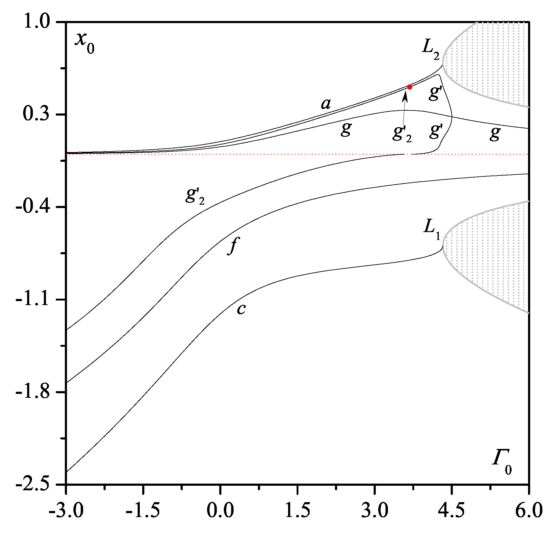
By applying the grid search and the aforementioned predictor-corrector techniques we have computed the basic families of planar symmetric periodic orbits of the classical Hill problem. The resulting family characteristics in the plane of initial conditions $({\Gamma }_0,x_0)$ are shown in Figure 1. We note here that, for the Hill problem the respective families have been firstly computed and presented by Hénon [23] but we recompute them here in order to detect appropriate initial conditions for the VSR orbits (which had not been determined in that paper) which will be used as seed for their accurate computation. Also, for each computed family we keep the name which had been given by Hénon.

We now deal with the VC as well as the VSR orbits at which families of three-dimensional periodic orbits bifurcate. Our aim is to compute them with a predetermined accuracy, e.g., $0.5\times {10}^{-8},$ and use them as appropriate starting points for the determination of the corresponding bifurcating families of spatial periodic orbits. So, at the half number of the total crossings of a planar symmetric orbit with the Ox-axis, i.e., at its half period $t=T/2,$ the orbit will be considered to be periodic and VC or VSR if it simultaneously fulfills the following conditions:

$${\dot{x}}_{cut}(x_0,0,0,0,{\dot{y}}_0,0)=0,a_v(x_0,0,0,0,{\dot{y}}_0,0)=d,$$

(17)

where d may take the values $-1,-1/2,0$ and $1,$ which correspond to the specific bifurcations of the family of planar periodic orbits with a family of spatial periodic orbits which initially have the double, triple, quadruple or the same period with that of the planar one, respectively. These particular values of d are obtained directly from the relevant relations (11) and (12). If the above conditions do not hold we look for appropriate corrections $\delta x_0$ and $\delta {\dot{y}}_0$ of the initial conditions such that to fulfill (17). Expanding the arising equations in Taylor series and keeping only the linear terms we get:

$${\displaystyle \frac{\partial {\dot{x}}_{cut}}{\partial x_0}\delta x_0+\frac{\partial {\dot{x}}_{cut}}{\partial {\dot{y}}_0}\delta {\dot{y}}_0=-{\dot{x}}_{cut},\frac{\partial a_v}{\partial x_0}\delta x_0+\frac{\partial a_v}{\partial {\dot{y}}_0}\delta {\dot{y}}_0=d-a_v,}$$

(18)

from which we obtain the corrector system.

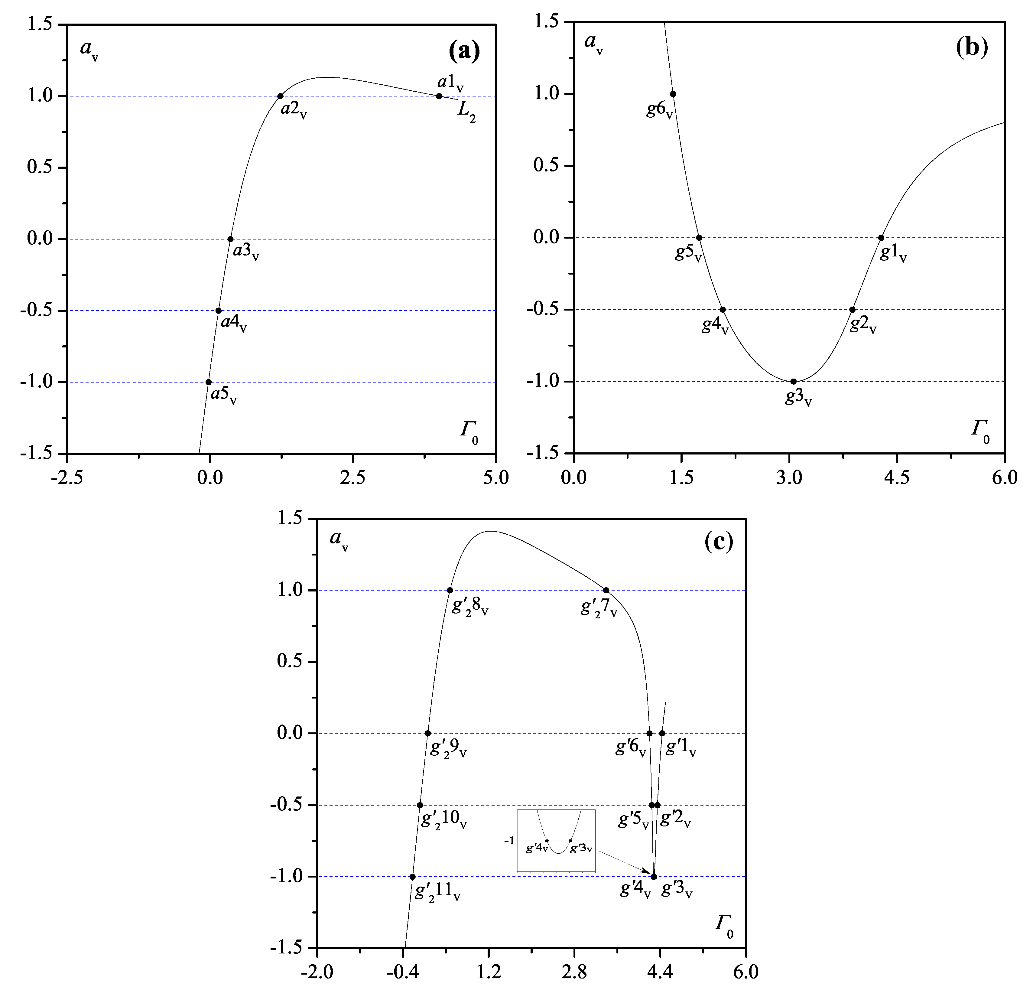
In Figure 2 we present the vertical stability diagrams of all the computed families. In particular, in Figure 2a we show the vertical stability of the Lyapunov family a emanating from the collinear equilibrium point $L_2$. Due to the symmetry of the classical Hill problem with respect to both axes the corresponding stability diagram of the second Lyapunov family c emanating from the other collinear equilibrium point $L_1$ is the same; therefore it is not presented here separately. As we see, there are three VC orbits, denoted by $a{1}_v,$ $a{2}_v$ and $a{5}_v$, from which two families of 3D periodic orbits of the same period and one family of such orbits of double period bifurcate. Also, one VSR orbit exists (denoted by $a{4}_v$) from which a family of spatial periodic orbits of triple period bifurcates and one VSR orbit ($a{3}_v$) from which a family of 3D periodic orbits of quadruple period bifurcates.

In Figure 2b the vertical stability diagram of family g is shown. For this family we observe that there are six VC and VSR periodic orbits. Specifically, at the VC orbit $g{3}_v$ a family of 3D periodic orbits of double period bifurcate while at $g{6}_v$ the 3D members of the bifurcated family are of the same period. Note here that, the stability curve of this family is tangential to the line $a_v=-1$ at its VC orbit $g{3}_v$ providing that this VC orbit is a double root. In addition, in this frame we see the existence of two VSR orbits ($g{2}_v$ and $g{4}_v$) at which two families of spatial periodic orbits of triple period bifurcate as well as two VSR orbits ($g{1}_v$ and $g{5}_v$) at which families of spatial periodic orbits of the quadruple period bifurcate.

Finally, in Figure 2c, the vertical stability of family $g^{\prime }$ is depicted. In this figure, it can be seen that there are five VC and six VSR periodic orbits. Two VC orbits ($g_2^{\prime }{7}_v$ and $g_2^{\prime }{8}_v$) give rise to two families of spatial periodic orbits of the same period while three VC orbits ($g^{\prime }{3}_v,$ $g^{\prime }{4}_v$ and $g_2^{\prime }{11}_v$) give rise to three such families whose members have the double period. Additionally, from the VSR orbits $g^{\prime }{2}_v,$ $g^{\prime }{5}_v$ and $g_2^{\prime }{10}_v$ three families of spatial periodic orbits of triple period bifurcate while from the VSR orbits $g^{\prime }{1}_v,$ $g^{\prime }{6}_v$ and $g_2^{\prime }{9}_v$ three families of such orbits bifurcate whose member orbits have the quadruple period. We note also here that, all the VC orbits had been determined in [24] but none of the VSR orbits and we choose to present them also here for the completeness of our study as well as for reader’s convenience. Additionally, we note here, that family f does not possess any VSR orbits with $q=3$ or $q=4$ in relation (12), therefore we do not show its vertical stability diagram.

Accurate initial conditions of the determined VC and VSR orbits of families $a,$ g and $g^{\prime }$ are given in

Table 1. VC and VSR orbits of families $a$, g and $g^{\prime }$. Due to the symmetry w.r.t. both axes the corresponding orbits of the Lyapunov family c emanating from the other equilibrium point $L_1$ are obtained directly from the Lyapunov family a; so, they are not given here.

Orbit	$\mathit{T}/2$	${\mathit{x}}_0$	${\dot{\mathit{y}}}_0$	${\mathbf{\Gamma }}_0$	${\mathit{x}}_{\mathit{c}\mathit{u}\mathit{t}}$	${\mathit{a}}_{\mathit{v}}-{\mathit{d}}_{\mathit{v}}$	${\mathit{b}}_{\mathit{v}}$	${\mathit{c}}_{\mathit{v}}$
$a{1}_v$	$1.54072125$	$0.58126467$	$0.67012429$	$4.00531265$	$0.77465745$	$1.000$	$-0.083$	$0.000$
$a{2}_v$	$2.06338271$	$0.21266090$	$2.88309804$	$1.22806326$	$0.94913598$	$1.000$	$0.000$	$-30.662$
$a{3}_v$	$2.54074663$	$0.12430197$	$3.97250147$	$0.35543401$	$1.10262083$	$0.000$	$0.019$	$-53.643$
$a{4}_v$	$2.69141465$	$0.10657722$	$4.31885774$	$0.14727997$	$1.16098760$	$-0.500$	$0.020$	$-37.453$
$a{5}_v$	$2.82554541$	$0.09298784$	$4.64365350$	$-0.02938892$	$1.21816343$	$-1.000$	$0.020$	$0.000$
$g{1}_v$	$0.70912134$	$0.30115821$	$1.62301941$	$4.27892454$	$-0.30115821$	$0.000$	$0.138$	$-7.268$
$g{2}_v$	$0.94220945$	$0.32764501$	$1.59674819$	$3.87661638$	$-0.32764501$	$-0.500$	$0.127$	$-5.911$
$g{3}_v$	$1.47270071$	$0.31084341$	$1.91481277$	$3.05747078$	$-0.31084341$	$-1.000$	$0.000$	$0.000$
$g{4}_v$	$2.05558702$	$0.22845003$	$2.61489589$	$2.07353736$	$-0.22845003$	$-0.500$	$-0.071$	$10.511$
$g{5}_v$	$2.27921091$	$0.19822182$	$2.90881626$	$1.74637033$	$-0.19822182$	$0.000$	$-0.082$	$12.237$
$g{6}_v$	$2.56862675$	$0.16471506$	$3.29248839$	$1.38309359$	$-0.16471506$	$1.000$	$-0.089$	$0.000$
$g^{\prime }{1}_v$	$0.67152649$	$0.39943360$	$1.02470483$	$4.43571163$	$-0.18804330$	$0.000$	$0.229$	$-4.371$
$g^{\prime }{2}_v$	$0.80598291$	$0.49144348$	$0.66802090$	$4.34794216$	$-0.13202001$	$-0.500$	$0.264$	$-2.846$
$g^{\prime }{3}_v$	$1.05140046$	$0.57085389$	$0.44267629$	$4.28518367$	$-0.08646195$	$-1.000$	$0.000$	$-0.328$
$g^{\prime }{4}_v$	$1.08318636$	$0.57696026$	$0.42952310$	$4.28060260$	$-0.08221610$	$-1.000$	$-0.051$	$0.000$
$g^{\prime }{5}_v$	$1.32511737$	$0.60237171$	$0.40729155$	$4.24287767$	$-0.05283047$	$-0.500$	$-0.387$	$1.938$
$g^{\prime }{6}_v$	$1.45376790$	$0.60041876$	$0.46088083$	$4.20010544$	$-0.03615817$	$0.000$	$-0.439$	$2.277$
$g_2^{\prime }{7}_v$	$1.81528649$	$0.46469701$	$1.24961994$	$3.39015957$	$-0.00439928$	$1.000$	$-0.179$	$0.000$
$g_2^{\prime }{8}_v$	$3.48496672$	$0.11419691$	$4.13226025$	$0.47715701$	$-0.28581588$	$1.000$	$0.000$	$-104.825$
$g_2^{\prime }{9}_v$	$4.08061376$	$0.07884361$	$5.03211914$	$0.06309927$	$-0.35442155$	$0.000$	$0.008$	$-123.893$
$g_2^{\prime }{10}_v$	$4.30312817$	$0.06856493$	$5.40976067$	$-0.08197783$	$-0.38101203$	$-0.500$	$0.009$	$-84.427$
$g_2^{\prime }{11}_v$	$4.51230096$	$0.05994922$	$5.79584998$	$-0.21952852$	$-0.40811555$	$-1.000$	$0.009$	$0.000$

. In particular, in this table, we give the half of the orbit’s period $T/2$, the position and velocity components $x_0$ and ${\dot{y}}_0$ at the initial vertical intersection of the VC or VSR orbit with the Ox-axis (this means that the remaining components of the position and velocity vectors are $y_0=0$ and ${\dot{x}}_0=0$), respectively, as well as the value of the Jacobi constant ${\Gamma }_0$ as it is computed through Equation (3) of the integral of motion for $(x_0,0,0,{\dot{y}}_0)$. Finally, we present the value of the position $x_{cut}$ at the second orbit’s vertical intersection with the Ox-axis while in the last three columns of the table we incorporate the vertical stability indices $a_v,$ $b_v,$ $c_v$ and $d_v,$ as they are determined by variations (10) and their values define the kind of the vertical bifurcation that occurs at a specific VSR planar periodic orbit.

3. Spatial Periodic Orbits

The VSR orbits give rise to families of three-dimensional periodic orbits which may possess all possible types of symmetry. In particular, the multiplicity q, as it is defined in (12), determines the symmetry properties of the generated spatial periodic orbits. These orbits possess, at least initially, the period $qT,$ where T is the whole period of a VSR orbit. Additionally, at each VSR orbit two branches of spatial periodic orbits bifurcate, i.e., from VSR orbits families always occur in pairs. This has been firstly identified by Robin and Markellos [38] who also described the mechanism where the spatial periodic orbits branch out from the plane. They pointed out that at a VSR orbit, i.e., $q\ge 3,$ exactly two branches of three-dimensional periodic orbits bifurcate while their symmetry properties depend on their own multiplicity. Specifically, in case that the generated spatial periodic orbits are of:

• Odd multiplicity q, i.e., their period is $(2n+1)T,$ $q=2n+1,$ $n=1,2,\dots ,$ with T being the VSR orbit’s period, two such families branch out from the corresponding VSR orbit; one family consists of axis-axis symmetric periodic orbits while the members of the other family are plane-plane symmetric. More precisely, each branch has one of the following symmetries:

  (a)

  O$x-$ Ox symmetry, i.e., they are axisymmetric spatial periodic orbits. They start on the Ox-axis with initial conditions of the form $(x_0,0,0,0,{\dot{y}}_0,{\dot{z}}_0)$ while at their half period $T/2$ return on this axis with final conditions of the form $(x_{cut},0,0,0,{\dot{y}}_{cut},{\dot{z}}_{cut})$.

  (b)

  O$xz-$ O$xz$ symmetry, i.e., they are plane symmetric spatial periodic orbits. They start on the O$xz-$ plane with initial conditions of the form $(x_0,0,z_0,0,{\dot{y}}_0,0)$ while at their half period $T/2$ return on this plane perpendicularly with final conditions $(x_{cut},0,z_{cut},0,{\dot{y}}_{cut},0)$.

• Even multiplicity q, i.e., their period is $\left(2n\right)T,$ $q=2n,$ $n=2,3,\dots ,$ with T being the VSR orbit’s period, two families branch out from the corresponding VSR orbit; both of them consist of orbits which are doubly symmetric according to the following characteristics:

  (a)

  O$x-$ O$xz$ symmetry, i.e., they are doubly symmetric spatial periodic orbits. They start on the Ox-axis with initial conditions of the form $(x_0,0,0,0,{\dot{y}}_0,{\dot{z}}_0)$ while at the quarter of their period $T/4$ return perpendicularly on the O$xz-$ plane with the final conditions $(x_{cut},0,z_{cut},0,{\dot{y}}_{cut},0)$.

  (b)

  O$xz-$ Ox symmetry, i.e., they are also doubly symmetric spatial periodic orbits. However, now they start on the O$xz-$ plane with initial conditions of the form $(x_0,0,z_0,0,{\dot{y}}_0,0)$ while at the quarter of their period $T/4$ return on the Ox-axis with the final conditions $(x_{cut},0,0,0,{\dot{y}}_{cut},{\dot{z}}_{cut}),$ respectively.

For the computation of these branches we can construct corrector-predictor algorithms based on the periodicity conditions. So, to compute a three-dimensional periodic orbit of type, e.g., O$x-$ O$xz$ double symmetry (case 2(a) above) we choose an initial state vector of the form ${\mathbf{x}}_{\mathbf{0}}=(x_0,0,0,0,{\dot{y}}_0,{\dot{z}}_0)$. In this case, at the quarter $T/4$ of the period, namely the orbit meets the O$xz-$ plane, the following conditions must be hold:

$$\begin{array}{c}{\dot{x}}_{cut}(x_0,0,0,0,{\dot{y}}_0,{\dot{z}}_0)=0,\hfill \\ {\dot{z}}_{cut}(x_0,0,0,0,{\dot{y}}_0,{\dot{z}}_0)=0,\hfill \end{array}$$

(19)

i.e., the orbit has to cross perpendicularly the O$xz-$ plane in order the periodicity to be established. In general, these are not satisfied, so we seek appropriate corrections $\delta x_0,$ $\delta {\dot{y}}_0$ and $\delta {\dot{z}}_0$ of the initial conditions. Then, the resulting equations are expanded in Taylor series up to first order terms obtaining:

$$\begin{array}{c}{\displaystyle {\dot{x}}_{cut}+\frac{\partial {\dot{x}}_{cut}}{\partial x_0}\delta x_0+\frac{\partial {\dot{x}}_{cut}}{\partial {\dot{y}}_0}\delta {\dot{y}}_0+\frac{\partial {\dot{x}}_{cut}}{\partial {\dot{z}}_0}\delta {\dot{z}}_0=0,}\hfill \\ {\displaystyle {\dot{z}}_{cut}+\frac{\partial {\dot{z}}_{cut}}{\partial x_0}\delta x_0+\frac{\partial {\dot{z}}_{cut}}{\partial {\dot{y}}_0}\delta {\dot{y}}_0+\frac{\partial {\dot{z}}_{cut}}{\partial {\dot{z}}_0}\delta {\dot{z}}_0=0.}\hfill \end{array}$$

(20)

Since we have two simultaneous equations with three unknowns, we choose to fix one of them, e.g., $\delta {\dot{z}}_0=0,$ and solve for obtaining the remaining corrections. In this case, these are:

$${\displaystyle \delta x_0=\frac{v_{45}{\dot{z}}_{cut}-v_{65}{\dot{x}}_{cut}}{v_{41}{v}_{65}-v_{45}{v}_{61}},\delta {\dot{y}}_0=\frac{v_{61}{\dot{x}}_{cut}-v_{41}{\dot{z}}_{cut}}{v_{41}{v}_{65}-v_{45}{v}_{61}},}$$

(21)

where the partial derivatives $v_{41}=\partial {\dot{x}}_{cut}/\partial x_0,$ $v_{45}=\partial {\dot{x}}_{cut}/\partial {\dot{y}}_0,$ $v_{61}=\partial {\dot{z}}_{cut}/\partial x_0$ and $v_{65}=\partial {\dot{z}}_{cut}/\partial {\dot{y}}_0$ are elements of the variational matrix given in (8). By iterating this process the three-dimensional periodic solution will be computed with the desired accuracy. If a spatial periodic orbit has been sought, i.e., conditions (19) are fulfilled with a predetermined accuracy, a next such orbit existing in its neighbourhood can be predicted. To do so, we use the linearized system (20) and slightly change $\Delta {\dot{z}}_0$ to an arbitrarily chosen small constant $\epsilon$ in order to get the remaining predictions in the form:

$${\displaystyle \Delta x_0=\frac{v_{45}{v}_{66}-v_{46}{v}_{65}}{v_{41}{v}_{65}-v_{45}{v}_{61}}\epsilon ,\Delta {\dot{y}}_0=\frac{v_{46}{v}_{61}-v_{41}{v}_{66}}{v_{41}{v}_{65}-v_{45}{v}_{61}}\epsilon ,}$$

(22)

where in system (20) we have now set $\delta x_0\equiv \Delta x_0,$ $\delta {\dot{y}}_0\equiv \Delta {\dot{y}}_0$ and $\delta {\dot{z}}_0\equiv \Delta {\dot{z}}_0$ to distinguish the prediction and correction steps. Also, the new terms appeared in (22) are $v_{46}=\partial {\dot{x}}_{cut}/\partial {\dot{z}}_0$ and $v_{66}=\partial {\dot{z}}_{cut}/\partial {\dot{z}}_0$.

The stability of a three-dimensional periodic orbit can be determined through the variational Equation (7) and using the following formulas [38]:

$$P=\frac{\alpha +\sqrt{{\alpha }^2-4(\beta -2)}}{2},Q=\frac{\alpha -\sqrt{{\alpha }^2-4(\beta -2)}}{2},$$

(23)

with $\alpha =2-\mathrm{Tr}\left(V\right)$ and $\beta =({\alpha }^2+2-\mathrm{Tr}{\left(V\right)}^2)/2,$ while V is the variational matrix given in (8), computed at the orbit’s period T. In this case, the periodic orbit in question is stable if the defined parameters $P,$ Q of (23) are reals for which it simultaneously holds $\left|P\right|<2$ and $\left|Q\right|<2$. Note that, we can also exploit the symmetry properties of the periodic orbit so as to determine the variational matrix at the half or the quarter of the period $T,$ i.e., $T_1=T/2$ or $T_2=T/4,$ depending on whether it possesses a simple or double symmetry, respectively. In particular, for the simple types of symmetry we get the variational matrix by using the following two formulas [38]:

$$V\left(T\right)=M{V}^{-1}\left(T_1\right)MV\left(T_1\right),V\left(T\right)=L{V}^{-1}\left(T_1\right)LV\left(T_1\right),$$

(24)

where the first one corresponds to the O$x-$ Ox type of symmetry and the second holds for the O$xz-$ O$xz$ plane one. Finally, for the orbits of double symmetry we have that:

$$V\left(T\right)={\left[M{V}^{-1}\left(T_2\right)LV\left(T_2\right)\right]}^2,V\left(T\right)={\left[L{V}^{-1}\left(T_2\right)MV\left(T_2\right)\right]}^2.$$

(25)

The first formula fits to the O$x-$ O$xz$ double symmetry while the second to the O$xz-$ Ox one. In all the above mentioned cases, $L,$ M are the diagonal matrices $L=\mathrm{diag}\{1,-1,1,-1,1,-1\}$ and $M=\mathrm{diag}\{1,-1,-1,-1,1,1\},$ respectively. Obviously, the determination of the variational matrix through transformations (24) and (25) offers economy to the computations of the numerical integration.

So, by applying the above mentioned techniques we have determined twenty four families of three-dimensional periodic orbits, together with their stability properties, which bifurcate from the VSR orbits given in Table 1. Note that, the corresponding families where the VC orbits, of the same table, generate have been discussed by Batkhin and Batkhina [37], so we do not consider their study here. Specifically, Table 1 contains twelve VSR periodic orbits; each one of these planar orbits possesses two vertical intersections with the Ox-axis (given in this table as $x_0$ and $x_{cut}$, respectively) so as a mirror configuration to be satisfied [45]. Twelve families of three-dimensional periodic orbits branch from the first vertical intersection of a VSR orbit while the rest twelve spatial families are generated from the second intersection of the same VSR orbit. All these branches of spatial periodic orbits have been computed and followed to their natural end.

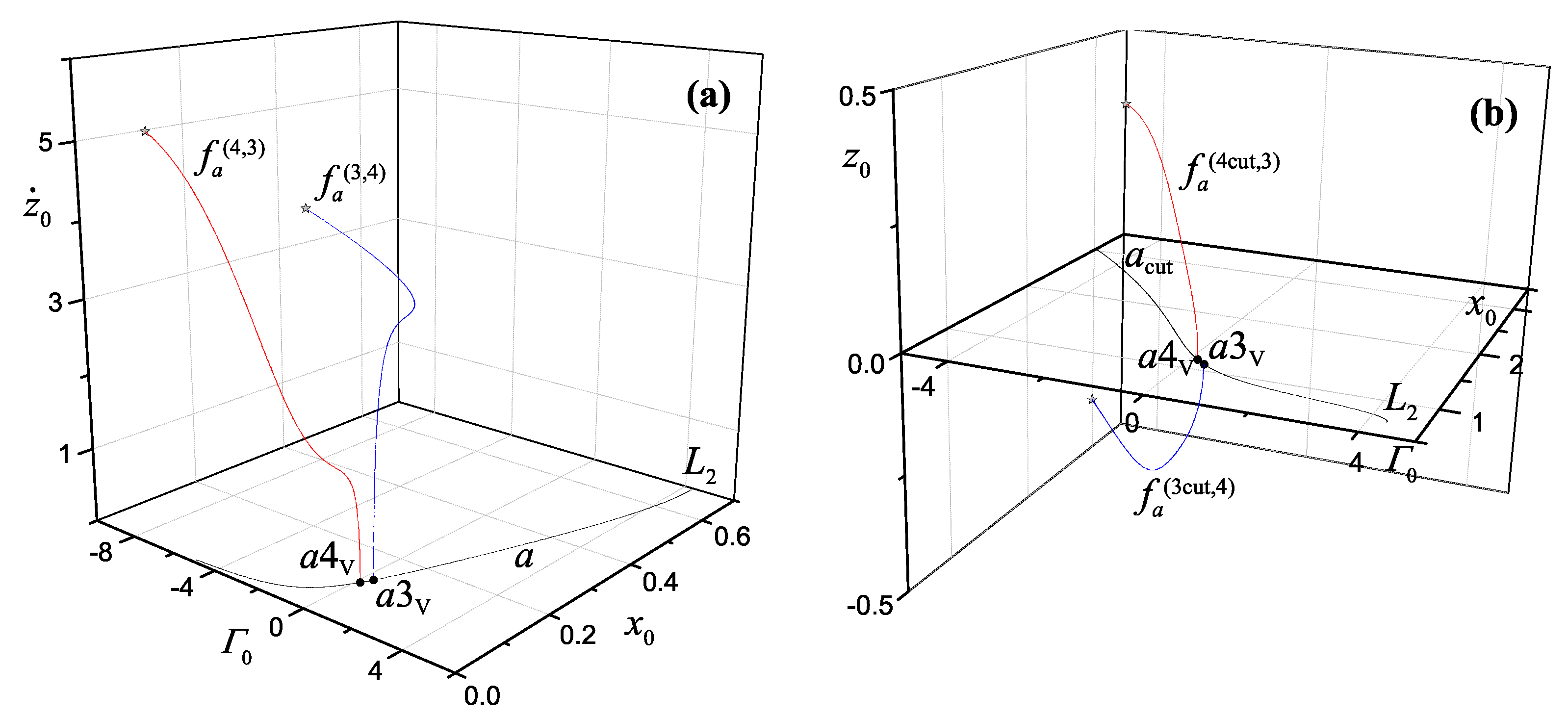
The planar Lyapunov family a has two VSR orbits under consideration at which four families of spatial periodic orbits bifurcate. These are shown in Figure 3 where we have plotted their characteristic curves in the space of their initial conditions. Families $f_a^{(3,4)}$ and $f_a^{(4,3)}$ bifurcate from the first perpendicular intersections of $a{3}_v$ and $a{4}_v$ VSR orbits, respectively, while the second such intersections give rise to the families $f_a^{(3cut,4)}$ and $f_a^{(4cut,3)},$ correspondingly. In the superscript, the first number follows the running number of the corresponding VSR orbit while the second one indicates that the period of the spatial periodic orbits is, at least initially, $qT,$ $q=3$ or $4,$ where T is the period of the VSR orbit, i.e., it describes the period commensurability between the planar and spatial orbits.

More precisely, in the first frame of Figure 3 we present the characteristic curve of the planar family a by giving its initial conditions $({\Gamma }_0,x_0),$ where the value of the Jacobi constant ${\Gamma }_0$ is determined by (3) for $x_0,$ $y_0=0,$ $z_0=0,$ ${\dot{x}}_0=0,$ ${\dot{y}}_0$ and ${\dot{z}}_0=0$ (first perpendicular cuts of family’s orbits with the Ox-axis), while the second frame depicts the respective characteristic curve in the $({\Gamma }_0,x_{cut})$ plane, i.e., these conditions correspond to the second perpendicular cuts $x_{cut},$ $y_{cut}=0,$ $z_{cut}=0,$ ${\dot{x}}_{cut}=0,$ ${\dot{y}}_{cut}$ and ${\dot{z}}_{cut}=0$ of the planar orbits with the Ox-axis (obviously it holds ${\Gamma }_0\equiv {\Gamma }_c$). Also, according to the multiplicity q, family $f_a^{(4,3)}$ consists of axisymmetric spatial periodic orbits and family $f_a^{(4cut,3)}$ of plane symmetric ones while families $f_a^{(3,4)}$ and $f_a^{(3cut,4)}$ have spatial members which are doubly symmetric. All the computed families go to three-dimensional collision orbits, so we consider that this is their natural termination and stop calculating them.

In Figure 4 the corresponding spatial branches which the planar family g generates are presented. This family possesses four VSR orbits therefore, eight such branches bifurcate. For their names we follow the same terminology described in the previous paragraph. So, $g{1}_v$ gives rise to families $f_g^{(1,4)}$ and $f_g^{(1cut,4)}$ which consist of doubly symmetric spatial members and both of them terminate with co-planar periodic orbits. Families $f_g^{(5,4)}$ and $f_g^{(5cut,4)}$ bifurcate from $g{5}_v$ and due to their orbit’s multiplicity they are also comprised by orbits of double symmetry. Both of them goes to three-dimensional collision orbits. Finally, families $f_g^{(2,3)},$ $f_g^{(2cut,3)}$ and $f_g^{(4,3)},$ $f_g^{(4cut,3)}$ are produced by the VSR orbits $g{2}_v$ and $g{4}_v,$ respectively. The spatial member orbits of branches $f_g^{(2,3)}$ and $f_g^{(4,3)}$ are axisymmetric while the corresponding members of families $f_g^{(2cut,3)}$ and $f_g^{(4cut,3)}$ are plane symmetric. The last four families terminate on the plane.

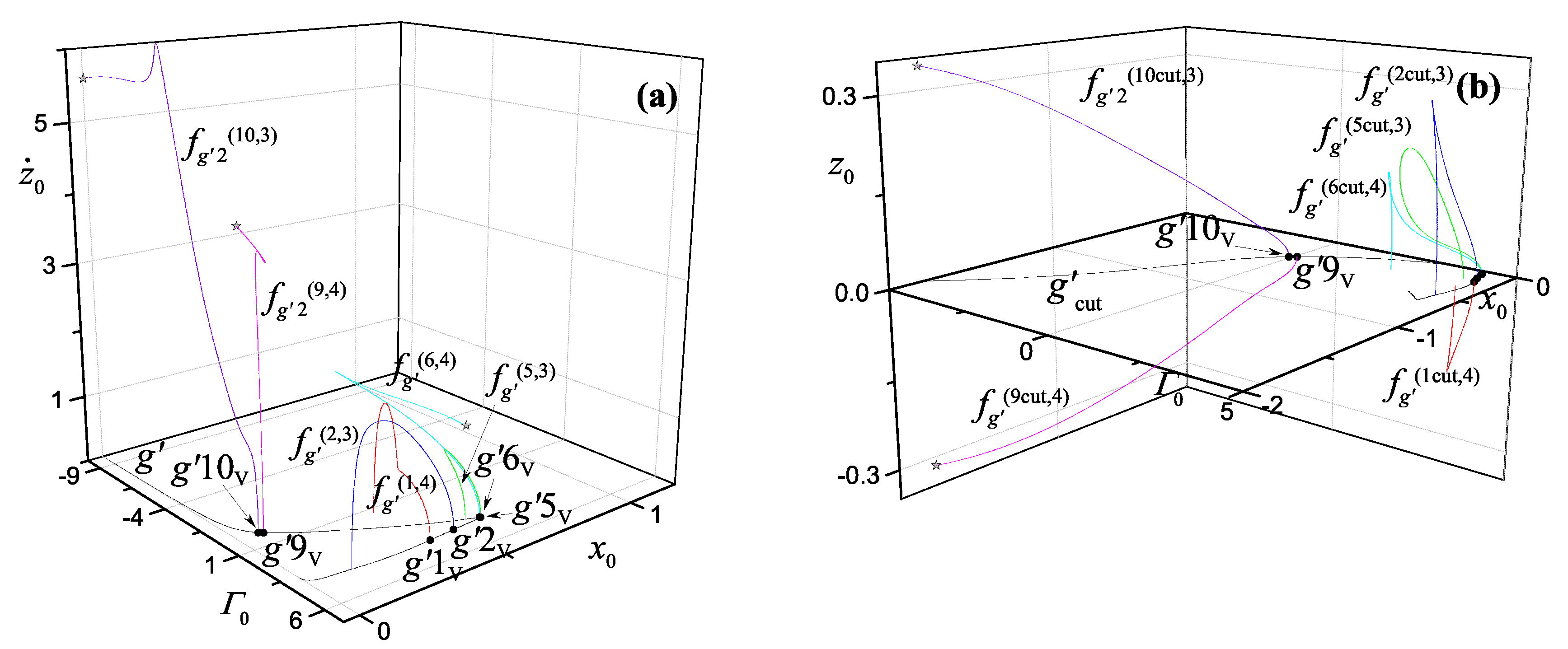
All families of three-dimensional periodic orbits which bifurcate from the VSR orbits of the planar family $g^{\prime }$ and their members have initially multiplicities 3 and 4 are presented in Figure 5. The six VSR orbits $g^{\prime }{i}_v,$ $i=1,2,5,6,9$ and $10,$ of $g^{\prime }$ which have been spotted indicate that, in total, twelve vertical branches intersect them. In particular, the branched families $f_{g^{\prime }}^{(2,3)},$ $f_{g^{\prime }}^{(5,3)}$ and $f_{g^{\prime }2}^{(10,3)}$, which are generated from the first vertical intersections of the VSR orbits $g^{\prime }{2}_v,$ $g^{\prime }{5}_v$ and $g_2^{\prime }{10}_v,$ respectively, consist of three-dimensional members which admit the O$x-$ Ox axis symmetry. Moreover, the first two families terminate on the O$xy-$ plane with coplanar orbits while the third one goes to a collision orbit in three-dimensions. The second vertical intersections of these VSR orbits give rise to the families $f_{g^{\prime }}^{(2cut,3)},$ $f_{g^{\prime }}^{(5cut,3)}$ and $f_{g^{\prime }2}^{(10cut,3)}$ whose member orbits possess the O$xz-$ O$xz$ plane symmetry. Furthermore, the first two families fall on planar periodic orbits and eventually cease to exist in three-dimensions while the rest one is led to spatial collision orbits. Besides, families $f_{g^{\prime }}^{(1,4)},$ $f_{g^{\prime }}^{(6,4)}$ and $f_{g^{\prime }2}^{(9,4)},$ emerge from the VSR orbits $g^{\prime }{1}_v,$ $g^{\prime }{6}_v$ and $g_2^{\prime }{9}_v,$ respectively, and they are constituted by orbits of the double symmetry O$x-$ O$xz$. The first family terminate on the plane while the rest two go to collision orbits. Finally, the same VSR orbits give also rise to the branches $f_{g^{\prime }}^{(1cut,4)},$ $f_{g^{\prime }}^{(6cut,4)}$ and $f_{g^{\prime }2}^{(9cut,4)},$ respectively, where the first two end on the plane while the third one goes, in its evolution, to collision orbits. The member orbits of the latter families are O$xz-$ Ox doubly symmetric.

The terminations of the spatial families which were found to end on the physical plane O$xy$ are shown in Figure 6 with the cyan, green and magenta coloured dots. In this figure, we have plotted the basic families of planar symmetric periodic orbits along both the positive and negative direction of the flow, i.e., for $\dot{y}>0$ (black continuous lines) and $\dot{y}<0$ (blue dotted lines), respectively, providing thus a chart with all vertical intersections of the respective planar orbits with the Ox-axis. In particular, the green dots correspond to the terminations of families $f_g^{(2cut,3)}$ and $f_g^{(4cut,3)}$ where they end up with degenerated orbits around the primary body located at the origin. Furthermore, the magenta dots indicate the planar terminations of families $f_g^{(4,3)},$ $f_{g^{\prime }}^{(5cut,3)},$ $f_{g^{\prime }}^{(5,3)}$ and $f_{g^{\prime }}^{(6cut,4)}$. Specifically, family $f_g^{(4,3)}$ ends up on a planar family where its members are of multiplicity five (magenta dot near $L_2$), $f_{g^{\prime }}^{(5cut,3)}$ terminates on another family with planar periodic orbits of multiplicity three (magenta dot near the characteristic curve of f) while $f_{g^{\prime }}^{(5,3)}$ and $f_{g^{\prime }}^{(6cut,4)}$ end up also on planar families with members of multiplicity three (the magenta dots which are shown to be located on the characteristic curves of $g^{\prime }$ and $g_2^{\prime }$). The latter four cases of planar families have not been identified in our study since we have only considered the basic families of the Hill’s problem. Also, the two cyan dots on the characteristic curve of family f with $\dot{y}<0,$ i.e., family $f_{cut},$ correspond to the termination orbits of families $f_g^{(2,3)}$ and $f_{g^{\prime }}^{(1,4)}$. However, the first family bifurcates from a VSR orbit of the family $f_{cut}$ of retrograde satellites with $q=5$ in relation (12) while the second one emanates from a VSR orbit with $q=6$, two cases which have not also been considered in our study. The remaining five cyan dots located on the characteristic curves of $g^{\prime },$ $g_{cut}^{\prime }$ and $g_{cut}$ represent the terminations of families $f_{g^{\prime }}^{(2,3)},$ $f_{g^{\prime }}^{(2cut,3)},$ $f_g^{(1,4)},$ $f_g^{(1cut,4)}$ and $f_{g^{\prime }}^{(1cut,4)}$ which return on VSR orbits of these planar families (existing in Table 1) or on VSR orbits which are images of the latter ones under reflection in the origin and have the same value of the Jacobi constant $\Gamma$. In particular, families $f_{g^{\prime }}^{(2,3)}$ and $f_{g^{\prime }}^{(2cut,3)}$ end up on the two vertical intersections of the symmetrical VSR orbit of $g^{\prime }2v$. Also, $f_g^{(1,4)}$ terminates on the positive crossing of the image planar orbit of $g^{\prime }1v$ while $f_g^{(1cut,4)}$ falls on the vertical intersection $x_{cut}$ of $g^{\prime }1v$. Finally, $f_{g^{\prime }}^{(1cut,4)}$ falls on the vertical intersection $x_{cut}$ of $g1v$ from which $f_g^{(1cut,4)}$ originates, so these two families are essentially the same.

Table 2. Sample members of families of 3D periodic orbits having the O$x-$ Ox axis symmetry. These families bifurcate from the VSR orbits as the first column denotes. The last column indicates whether each family contains stable parts $\left(S\right)$ or not $\left(U\right)$.

VSR Orbit	Family	$\mathit{T}/2$	${\mathit{x}}_0$	${\dot{\mathit{y}}}_0$	${\dot{\mathit{z}}}_0$	${\mathbf{\Gamma }}_0$	Stability
$a{4}_v$	$f_a^{(4,3)}$	$8.28108914$	$0.09738337$	$4.35161692$	$1.30000000$	$-0.06073137$	U
$g{2}_v$	$f_g^{(2,3)}$	$3.02875641$	$0.36825238$	$0.02326322$	$1.73500119$	$2.82711705$	U
$g{4}_v$	$f_g^{(4,3)}$	$6.40350957$	$0.27206142$	$1.28603484$	$2.16710076$	$1.22312215$	U
$g^{\prime }{2}_v$	$f_{g^{\prime }}^{(2,3)}$	$2.71221891$	$0.24559916$	$1.30859807$	$1.72000000$	$3.65347819$	U
$g^{\prime }{5}_v$	$f_{g^{\prime }}^{(5,3)}$	$4.40022566$	$0.52395964$	$0.57439090$	$0.97702231$	$3.35619150$	U
$g_2^{\prime }{10}_v$	$f_{g^{\prime }2}^{(10,3)}$	$14.90408085$	$0.04362095$	$6.66929837$	$1.40386131$	$-0.59513059$	U

incorporates initial conditions for sample members of the six computed spatial families whose orbits are axisymmetric and have been generated from the VSR orbits $a4v,$ $g2v,$ $g4v,$ $g^{\prime }2v,$ $g^{\prime }5v$ and $g_2^{\prime }10v$. In particular, each entry involves the orbit’s half period $T/2$, the position and velocity components $(x_0,0,0,0,{\dot{y}}_0,{\dot{z}}_0)$ which the orbit has initially on the Ox-axis as well as the value of the Jacobi constant. The last column indicates whether the family contains some stable parts $\left(S\right)$ or not $\left(U\right)$. In

Table 3. Sample members of families of 3D periodic orbits having the O$xz-$ O$xz$ plane symmetry. These families bifurcate from the second vertical intersection with the Ox-axis of the corresponding VSR orbits, presented in the first column. The last column indicates whether each family contains stable parts $\left(S\right)$ or not $\left(U\right)$.

VSR Orbit	Family	$\mathit{T}/2$	${\mathit{x}}_0$	${\mathit{z}}_0$	${\dot{\mathit{y}}}_0$	${\mathbf{\Gamma }}_0$	Stability
$a{4}_v$	$f_a^{(4cut,3)}$	$8.10480019$	$1.17311668$	$0.05000000$	$-2.39299088$	$0.10301672$	U
$g{2}_v$	$f_g^{(2cut,3)}$	$2.94020264$	$-0.16401030$	$0.25153736$	$-1.87987761$	$3.14385103$	S
$g{4}_v$	$f_g^{(4cut,3)}$	$6.31311752$	$-0.13802904$	$0.12953972$	$-2.98949436$	$1.66882484$	U
$g^{\prime }{2}_v$	$f_{g^{\prime }}^{(2cut,3)}$	$2.86331675$	$-0.16518580$	$0.19202694$	$-2.13512698$	$3.38200526$	S
$g^{\prime }{5}_v$	$f_{g^{\prime }}^{(5cut,3)}$	$5.47054222$	$-0.04220315$	$0.10082891$	$-4.03567045$	$2.00597171$	U
$g_2^{\prime }{10}_v$	$f_{g^{\prime }2}^{(10cut,3)}$	$14.50221897$	$-0.47514046$	$0.05000000$	$2.31882339$	$-0.51599948$	U

we present sample members of the six families which bifurcate from the other vertical intersection of the same planar VSR orbits. Since their orbits are planar symmetric, we give now the position and velocity components $(x_0,0,z_0,0,{\dot{y}}_0,0)$ when the orbit starts perpendicularly from the O$xz-$ plane. Finally, in the

Table 4. Sample members of families of 3D periodic orbits having the O$x-$ O$xz$ double symmetry. These families bifurcate from the VSR orbits presented in the first column. The last column indicates whether each family contains stable parts $\left(S\right)$ or not $\left(U\right)$.

VSR Orbit	Family	$\mathit{T}/4$	${\mathit{x}}_0$	${\dot{\mathit{y}}}_0$	${\dot{\mathit{z}}}_0$	${\mathbf{\Gamma }}_0$	Stability
$a{3}_v$	$f_a^{(3,4)}$	$5.08770908$	$0.13256407$	$3.55142141$	$1.50000000$	$0.27716970$	U
$g{1}_v$	$f_g^{(1,4)}$	$1.43380965$	$0.29446412$	$1.34203629$	$1.08722851$	$4.06899919$	S
$g{5}_v$	$f_g^{(5,4)}$	$4.64387725$	$0.19337079$	$2.72154006$	$1.24600000$	$1.49570433$	U
$g^{\prime }{1}_v$	$f_{g^{\prime }}^{(1,4)}$	$1.36955543$	$0.38309726$	$1.04442285$	$0.50000000$	$4.32007783$	U
$g^{\prime }{6}_v$	$f_{g^{\prime }}^{(6,4)}$	$3.17340274$	$0.51995209$	$0.57763956$	$1.00000000$	$3.32389130$	U
$g_2^{\prime }{9}_v$	$f_{g^{\prime }2}^{(9,4)}$	$8.22922408$	$0.07940642$	$4.91666525$	$1.00000000$	$0.03219913$	U

and

Table 5. Sample members of families of 3D periodic orbits having the O$xz-$ Ox double symmetry. These families bifurcate from the second vertical intersection with the Ox-axis of the corresponding VSR orbits, presented in the first column. The last column indicates whether each family contains stable parts $\left(S\right)$ or not $\left(U\right)$.

VSR Orbit	Family	$\mathit{T}/4$	${\mathit{x}}_0$	${\mathit{z}}_0$	${\dot{\mathit{y}}}_0$	${\mathbf{\Gamma }}_0$	Stability
$a{3}_v$	$f_a^{(3cut,4)}$	$5.56514907$	$1.28678525$	$-0.19596176$	$-2.59789645$	$-0.28347259$	U
$g{1}_v$	$f_g^{(1cut,4)}$	$1.41364637$	$-0.22169375$	$-0.11327032$	$-2.00619479$	$4.14339700$	S
$g{5}_v$	$f_g^{(5cut,4)}$	$4.61712103$	$-0.16386318$	$0.08332496$	$-3.06307199$	$1.57070128$	U
$g^{\prime }{1}_v$	$f_{g^{\prime }}^{(1cut,4)}$	$1.43381518$	$-0.25279920$	$-0.14461255$	$-1.72308981$	$4.06898038$	S
$g^{\prime }{6}_v$	$f_{g^{\prime }}^{(6cut,4)}$	$2.91496122$	$-0.03575314$	$0.00564098$	$-7.14762756$	$4.17085491$	U
$g_2^{\prime }{9}_v$	$f_{g^{\prime }2}^{(9cut,4)}$	$9.16012429$	$-0.42750381$	$-0.04366273$	$2.34791591$	$-0.31222756$	U

we provide data for sample orbits of the families which the VSR orbits $a3v,$ $g1v,$ $g5v,$ $g^{\prime }1v,$ $g^{\prime }6v$ and $g_2^{\prime }9v$ generate from their two vertical intersections with the Ox-axis. The presented data correspond to the quarter of the orbits’ period $T/4$ since these families consist of spatial orbits which are doubly symmetric.

4. Conclusions

The Hill three-body problem was considered and its three-dimensional periodic solutions which bifurcate from the VSR periodic orbits of the basic planar families were determined. We focused on families where their spatial members have initially three or four times the period of a specific VSR planar orbit. Twelve such VSR orbits were detected and calculated accurately while these orbits were found to give rise to twenty four families of three-dimensional periodic orbits. As it happens in the classical restricted three-body problem, we also identified here that each VSR orbit may generate two vertical branches; each branch bifurcates from a vertical intersection of the planar VSR periodic orbit with the Ox-axis.

Besides, the multiplicity of the generated spatial orbit’s period was noticed to specify the symmetry properties of the orbit. Our results showed that the spatial orbits of the computed branches may have the following types of symmetry: axis-axis, plane-plane as well as double symmetry which combines both the other two types. The numerical continuation of these branches were accomplished through predictor-corrector algorithms which were based on mirror configurations where the periodicity conditions fulfill according to the spatial orbit’s type of symmetry. Thirteen branches were found to terminate with coplanar periodic orbits while the remaining eleven ones were collided in their evolution with the smaller primary body. Additionally, among the twenty four computed families of three-dimensional periodic orbits, we found that only five of them include stable parts; these are $f_g^{(2cut,3)},$ $f_{g^{\prime }}^{(2cut,3)},$ $f_g^{(1,4)},$ $f_g^{(1cut,4)}$ and $f_{g^{\prime }}^{(1cut,4)}$.

Since the vertical stability diagrams of the basic planar families indicated the existence of higher order resonances (than $q=4$ which was the maximum considered here) for the generation of vertical branches, a natural continuation of the present work would be to consider a similar study for their determination. Also, another interesting extension could be to incorporate additional forces in the Hill’s problem, such as the radiation of the larger primary body, i.e., the Sun emits radiation, and examine the influence of these forces to the considered here spatial solutions.

References

- Mingotti, G.; Topputo, F.; Bernelli-Zazzera, F. Earth-Mars transfers with ballistic escape and low-thrust capture. Celest. Mech. Dyn. Astr. 2011, 110, 169–188. [Google Scholar] [CrossRef] [Green Version]
- Capdevila, L.R.; Howell, K.C. A transfer network linking Earth, Moon, and the triangular libration point regions in the Earth-Moon system. Adv. Space Res. 2018, 62, 1826–1852. [Google Scholar] [CrossRef]
- Nagler, J. Crash test for the restricted three-body problem. Phys. Rev. E 2005, 71, 026227. [Google Scholar] [CrossRef] [Green Version]
- Zotos, E.E. Orbital dynamics in the planar Saturn-Titan system. Astrophys. Space Sci. 2015, 358, 4. [Google Scholar] [CrossRef] [Green Version]
- Antoniadou, K.I.; Veras, D. Driving white dwarf metal pollution through unstable eccentric periodic orbits. Astron. Astrophys. 2019, 629, A126. [Google Scholar] [CrossRef] [Green Version]
- Antoniadou, K.I.; Libert, A.-S. Spatial resonant periodic orbits in the restricted three-body problem. Mon. Not. R. Astron. Soc. 2019, 483, 2923–2940. [Google Scholar] [CrossRef]
- Douskos, C.; Kalantonis, V.; Markellos, P. Effects of resonances on the stability of retrograde satellites. Astrophys. Space Sci. 2007, 310, 245–249. [Google Scholar] [CrossRef]
- Gao, F.B.; Zhang, W. A study on periodic solutions for the circular restricted three-body problem. Astron. J. 2014, 148, 116. [Google Scholar] [CrossRef] [Green Version]
- Musielak, Z.; Quarles, B. Three body dynamics and its applications to exoplanets. In Springer Briefs in Astronomy; Springer: Cham, Switzerland, 2017. [Google Scholar]
- Voyatzis, G.; Antoniadou, K.I. On quasi-satellite periodic motion in asteroid and planetary dynamics. Celest. Mech. Dyn. Astr. 2018, 130, 59. [Google Scholar] [CrossRef] [Green Version]
- Abouelmagd, E.I.; Guirao, J.L.G.; Pal, A.K. Periodic solution of the nonlinear Sitnikov restricted three-body problem. New Astron. 2020, 75, 101319. [Google Scholar] [CrossRef]
- Antoniadou, K.I.; Voyatzis, G. Resonant periodic orbits in the exoplanetary systems. Astrophys. Space Sci. 2014, 349, 657–676. [Google Scholar] [CrossRef] [Green Version]
- Voyatzis, G.; Tsiganis, K.; Antoniadou, K.I. Inclined asymmetric librations in exterior resonances. Celest. Mech. Dyn. Astr. 2018, 130, 29. [Google Scholar] [CrossRef] [Green Version]
- Singh, J.; Perdiou, A.E.; Gyegwe, J.M.; Perdios, E.A. Periodic solutions around the collinear equilibrium points in the perturbed restricted three-body problem with triaxial and radiating primaries for binary HD 191408, Kruger 60 and HD 155876 systems. Appl. Math. Comput. 2018, 325, 358–374. [Google Scholar] [CrossRef]
- Pathak, N.; Abouelmagd, E.I.; Thomas, V.O. On higher order resonant periodic orbits in the photo-gravitational planar restricted three-body problem with oblateness. J. Astronaut. Sci. 2019, 66, 475–505. [Google Scholar] [CrossRef]
- Zotos, E.E.; Md Suraj, S.; Aggarwal, R.; Mittal, A. Orbit classification in the Copenhagen problem with oblate primaries. Astron. Nachr. 2019, 340, 760–770. [Google Scholar] [CrossRef]
- Gao, F.; Wang, R. Bifurcation analysis and periodic solutions of the HD 191408 system with triaxial and radiative perturbations. Universe 2020, 6, 35. [Google Scholar] [CrossRef] [Green Version]
- Zotos, E.E.; Dubeibe, F.L. Orbital dynamics in the post Newtonian planar circular restricted Sun-Jupiter system. Int. J. Mod. Phys. D 2018, 27, 1850036. [Google Scholar] [CrossRef] [Green Version]
- Zotos, E.E.; Chen, W.; Abouelmagd, E.I.; Han, H. Basins of convergence of equilibrium points in the restricted three-body problem with modified gravitational potential. Chaos Solitons Fractals 2020, 134, 109704. [Google Scholar] [CrossRef]
- Burgos-Garcia, J.; Bengochea, A. Horseshoe orbits in the restricted four-body problem. Astrophys. Space Sci. 2017, 362, 212. [Google Scholar] [CrossRef]
- Suraj, M.S.; Aggarwal, R.; Mittal, A.; Meena, O.P.; Asique, M.C. On the spatial collinear restricted four-body problem with non-spherical primaries. Chaos Solitons Fractals 2020, 133, 109609. [Google Scholar] [CrossRef]
- Hill, G.W. Researches in the lunar theory. Am. J. Math. 1878, 1, 5–26. [Google Scholar] [CrossRef]
- Hénon, M. Numerical exploration of the restricted problem V. Hill’s case: Periodic orbits and their stability. Astron. Astrophys. 1969, 1, 223–238. [Google Scholar]
- Hénon, M. Vertical stability of periodic orbits in the restricted problem II. Hill’s case. Astron. Astrophys. 1974, 30, 317–321. [Google Scholar]
- Zagouras, C.; Markellos, V.V. Three-dimensional periodic solutions around equilibrium points in Hill’s problem. Celes. Mech. 1985, 35, 257–267. [Google Scholar] [CrossRef]
- Hénon, M. New families of periodic orbits in Hill’s problem of three-bodies. Celest. Mech. Dyn. Astr. 2003, 85, 223–246. [Google Scholar] [CrossRef]
- Villac, B.F.; Scheeres, D.J. Escaping trajectories in the Hill three–body problem and applications. J. Guid. Control Dyn. 2003, 26, 224–232. [Google Scholar] [CrossRef]
- Kanavos, S.S.; Markellos, V.V.; Roy, A.E.; Perdios, E.A.; Douskos, C.N. The photogravitational Hill problem: Numerical exploration. Earth Moon Planets 2002, 91, 223–241. [Google Scholar] [CrossRef]
- Papadakis, K.E. The planar photogravitational Hill problem. Int. J. Bifurcat. Chaos 2006, 16, 1809–1821. [Google Scholar] [CrossRef]
- De Bustos, M.T.; Lopez, M.A.; Martinez, R.; Vera, J.A. On the periodic solutions emerging from the equilibria of the Hill Lunar problem with oblateness. Qual. Theory Dyn. Syst. 2018, 17, 331–344. [Google Scholar] [CrossRef]
- Markellos, V.V.; Roy, A.E.; Perdios, E.A.; Douskos, C.N. A Hill problem with oblate primaries and effect of oblateness on Hill stability of orbits. Astrophys. Space Sci. 2001, 278, 295–304. [Google Scholar] [CrossRef]
- Perdiou, A.E.; Markellos, V.V.; Douskos, C.N. The Hill problem with oblate secondary: Numerical exploration. Earth Moon Planets 2005, 97, 127–145. [Google Scholar] [CrossRef]
- Perdiou, A.E. Multiple periodic orbits in the Hill problem with oblate secondary. Earth Moon Planets 2008, 103, 105–118. [Google Scholar] [CrossRef]
- Papadakis, K.E. The planar Hill problem with oblate primary. Astrophys. Space Sci. 2004, 293, 271–287. [Google Scholar] [CrossRef]
- Perdiou, A.E.; Perdios, E.A.; Kalantonis, V.S. Periodic orbits of the Hill problem with radiation and oblateness. Astrophys. Space Sci. 2012, 342, 19–30. [Google Scholar] [CrossRef]
- Zotos, E.E. Comparing the fractal basins of attraction in the Hill problem with oblateness and radiation. Astrophys. Space Sci. 2017, 362, 190. [Google Scholar] [CrossRef] [Green Version]
- Batkhin, A.B.; Batkhina, N.V. Hierarchy of periodic solutions families of spatial Hill’s problem. Sol. Syst. Res. 2009, 43, 178–183. [Google Scholar] [CrossRef]
- Robin, I.A.; Markellos, V.V. Periodic orbits generated from vertical self-resonant satellite orbits. Celest. Mech. 1980, 21, 395–434. [Google Scholar] [CrossRef]
- Szebehely, V. Theory of Orbits; Academic Press: New York, NY, USA, 1967. [Google Scholar]
- Hénon, M. Vertical stability of periodic orbits in the restricted problem I. Equal masses. Astron. Astrophys. 1973, 28, 415–426. [Google Scholar]
- Markellos, V.V.; Black, W.; Moran, P.E. A grid search for families of periodic orbits in the restricted problem of three bodies. Celest. Mech. 1974, 9, 507–512. [Google Scholar] [CrossRef]
- Barrio, R.; Blesa, F. Systematic search of symmetric periodic orbits in 2DOF Hamiltonian systems. Chaos Solitons Fractals 2009, 41, 560–582. [Google Scholar] [CrossRef]
- Tsirogiannis, G.A.; Perdios, E.A.; Markellos, V.V. Improved grid search method: An efficient tool for global computation of periodic orbits: Application to Hill’s problem. Astrophys. Space Sci. 2009, 013, 49–78. [Google Scholar] [CrossRef]
- Zotos, E.E.; Papadakis, K.E. Orbit classification and networks of periodic orbits in the planar circular restricted five-body problem. Int. J. Nonlin. Mech. 2019, 111, 119–141. [Google Scholar] [CrossRef] [Green Version]
- Roy, A.E.; Ovenden, M.W. On the occurence of commensurable mean motions in the solar system: The mirror theorem. Mon. Not. R. Astron. Soc. 1955, 11, 296–309. [Google Scholar] [CrossRef] [Green Version]
Figure 1.
The basic families of planar periodic orbits of the Hill problem as they were determined in [23]—reproduction here. Forbidden regions to motion are shown with light grey color while red dashed line represents the position of the smaller primary body. The respective families have been recomputed here in order their VSR orbits to be calculated.
Figure 2.
Vertical stability diagrams of (a) family (b) family g and (c) family . and denote the VC or VSR orbits of the respective families.
Figure 3.
3D families bifurcating from the VSR orbits and of family a. (a) Bifurcating families starting from the initial condition of the planar family and (b) Bifurcating families starting from the initial condition of the planar family. Grey star indicates that a family goes to collision orbit.
Figure 4.
3D families bifurcating from the VSR orbits of family g. (a) Bifurcating families starting from the initial condition of the planar family and (b) Bifurcating families starting from the initial condition of the planar family. Grey star indicates that a family goes to collision orbit.
Figure 5.
3D families bifurcating from the VSR orbits of family . (a) Bifurcating families starting from the initial condition of the planar family and (b) Bifurcating families starting from the initial condition of the planar family. Grey star indicates that a family goes to collision orbit.
Figure 6.
The full chart of the basic families of planar periodic orbits of the Hill problem where both the positive (black continuous lines) and negative (blue dotted lines) crossings of the orbits with the Ox-axis are presented. Forbidden regions to motion are shown grey while red dashed line stands for the position of the secondary. Cyan, green and magenta dots represent the planar termination orbits of the spatial families.