Achieving Spatial Multi-Point Focusing by Frequency Diversity Array


1
Institute of Applied Physics, University of Electronic Science and Technology of China, Chengdu 611731, China
2
School of Electrical and Electronic Information, Xihua University, Chengdu 610039, China
3
Department of Electrical, Computers and Biomedical Engineering, University of Pavia, 27100 Pavia, Italy
*
Authors to whom correspondence should be addressed.
Electronics 2019, 8(8), 883; https://doi.org/10.3390/electronics8080883
Submission received: 5 July 2019
/
Revised: 30 July 2019
/
Accepted: 5 August 2019
/
Published: 9 August 2019
(This article belongs to the Section Microwave and Wireless Communications)
Abstract
:This paper proposes a class of frequency diverse array (FDA) for achieving time-varying spatial focusing for multiple targets. On the basis of single-target focusing of FDA, sequential focus at the four points is achieved by controlling the time period. The effects of frequency offset on the range of focusing area are derived. Since FDA is narrowband in nature, the relative operating bandwidth is limited to be 10%. Under the limitation of the bandwidth, the sequential multi-target focusing in the far-field is achieved. To validate the proposed method, numerical examples of eight-element FDA are reported and discussed.
1. Introduction
In 2006, P. Antonik and his colleagues first proposed the concept of frequency diversity array antenna based on the research of traditional beam-scanning phased array technique [1,2]. It is pointed out that by introducing a progressive small frequency offset at the center frequency of the array element, the pointing direction of the spatial beam will rotate with the change of the distance, thereby realizing the spatial beam scanning without the phase shifter. At the same year, they conducted a preliminary analysis of the relationship between distance and spatial beam of the frequency diversity array under waveform diversity. From 2008 to 2009, they studied the implementation of frequency diversity arrays, as well as frequency and amplitude-phase modulation methods and also verified the characteristics of beam pointing with distance variation of linear frequency offset of frequency diverse array (FDA) [3,4]. L. Huang et al. also designed an eight-element uniform linear array with linear frequency offset and tested its radiation characteristics [5]. The results show that the radiation beam of the array changes not only with the variation of the distance but also with the frequency offset. At the same time, the rate at which the beam scan angle changes with time is also obtained. In 2009, T. Higgins studied the linear frequency offset FDA. The research indicates that the half-power beam-width is narrowing as the frequency offset gradually increases [6]. It is also pointed out that the FDA can be used to improve the Doppler distance-ambiguity. There will be broad prospects in the field of imaging. In 2012, A. M. Jones extended the linear array of one-dimensional linear frequency offset to a two-dimensional planar array, and analyzed its distance-angle pattern characteristics [7]. In 2013, J. Shin used the finite difference time domain (FDTD) to perform time-domain full-wave analysis on FDA [8]. From 2007 to 2014 Demir et al. analyzed the spatial beam scanning characteristics of linear frequency-biased FDA and found that the beam scanning changes periodically in time, distance, and angle, and found the law of periodic variation [9,10,11].
The FDA have great potential to change the traditional information and energy transfer ways [12,13,14]. From 2017, researchers began to concentrate on the study of spatial focusing using FDA technology [15,16,17,18]. In 2017 A. M. Yao proposed time-modulated FDA for achieving spatial focusing for multiple areas [15]. The principle is based on modified time modulated optimized frequency offset. It allows the FDA available for fixed-point communication and the signal is not easily intercepted [16]. In the above studies, the focus spots produced by the FDA were time invariant [17,18]. If FDA can be used to generate multi-region time-varying focus, then the confidentiality of FDA communications can be further improved. Therefore, this paper will study the use of FDA to achieve multi-target time-varying focusing. In this paper, according to the theory of the single-target focusing of FDA, by optimizing the relevant parameters, time-varying multi-target focusing is achieved. By limiting the operating frequency band, the feeding signal of the array element cannot exceed the operation band.
2. Effects of Frequency Offset on the Range of Focusing Area
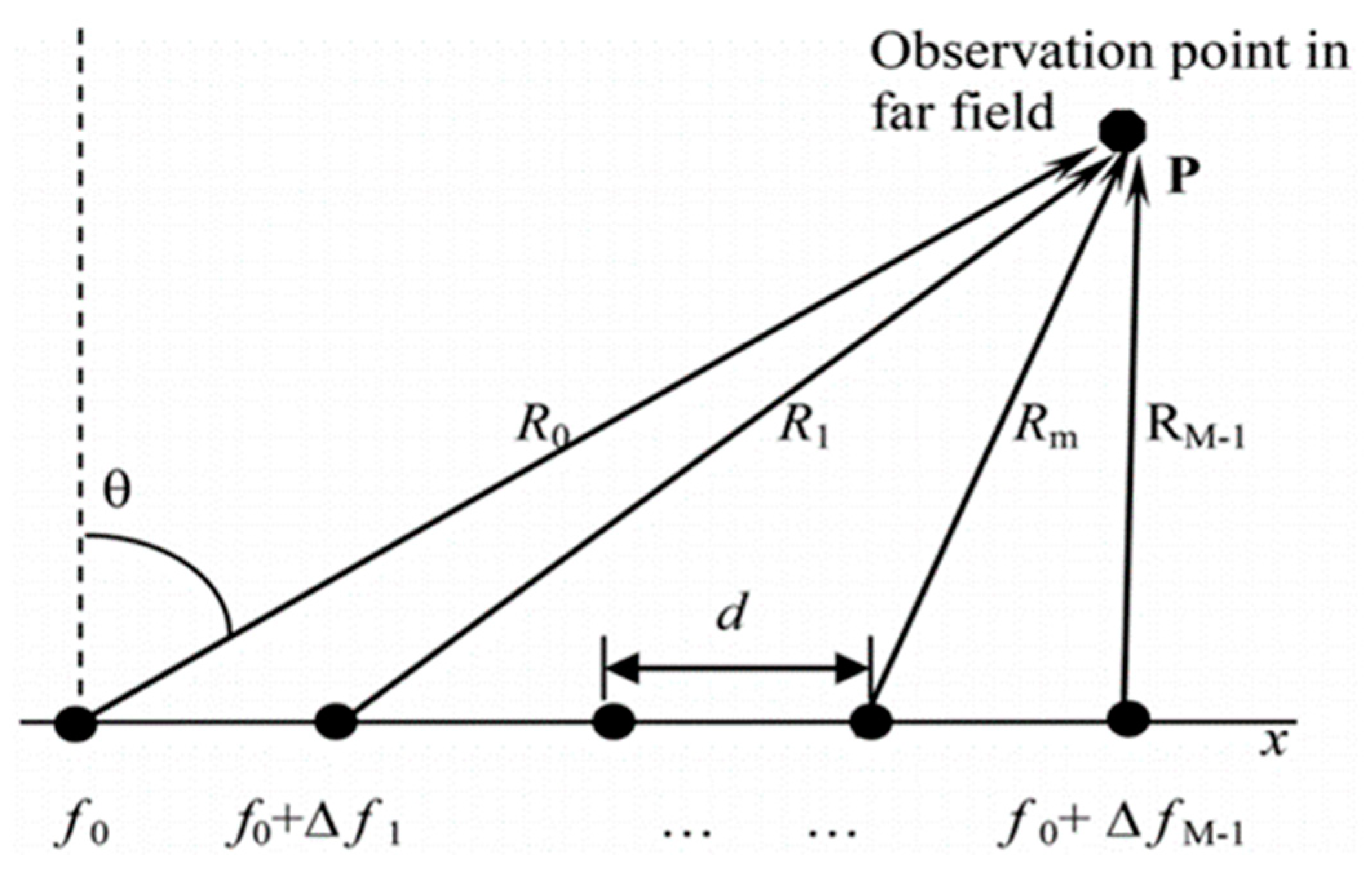
The schematic diagram is shown in Figure 1. The operating frequencies of the array elements are different. The position of the focusing point can be calculated with the classical equation of the FDA. However, the characteristics of the FDA impose limits on the far-field focus position. Once the limits are exceeded, the focusing behavior is adversely affected. In the case of an isotropic dipole introduced in Reference [15], for example, the array factor is
where f0 is the central operation frequency of the FDA, t is time, Δf is the frequency offset of the element, Rn is the distance from each element to the observation point in far field, and c is the speed of light in vacuum.
In considering the distance limitation, Rn represents the actual distance without any approximation, and g(n) is the corresponding array element parameter. To focus on the target area, we set the phase term of the exponent in Equation (1) to zero and obtain the following frequency offset [15]:
Since FDA is narrowband in nature, we assume a bandwidth of 10% and proceed with the following derivation on this basis.
2.1. The Frequency Offset is Negative
When the frequency offset is negative (), Equation (2) shows that, as time increases and with , (Rmin is the minimal distance) the absolute value of the denominator gradually decreases. Since the numerator remains the same and only the denominator changes, the absolute value of is the smallest at t = 0. When the corresponding frequency offset is zero, given that the denominator is negative and is negative, the numerator must be either positive or zero. Therefore, we have
From Equation (2), we have . If the value of t is smaller than and corresponds to , then we have
And
From simultaneous Equations (3) and (5), we obtain
Since , Equation (6) may be rewritten as
and we have
2.2. The Frequency Offset is Positive
Similarly, Equation (2) also shows that, as time progresses and with , the absolute value of the denominator gradually decreases. Since the numerator remains the same and only the denominator changes, the absolute value of is the smallest at t = 0. Hence, when the corresponding frequency offset is zero, given that the denominator is negative and is positive, the numerator must be either negative or zero. Therefore, we have
From Equation (2), we have . If the value of t is smaller than and corresponds to , then we have
And
From Equations (9) and (11), we obtain
Since , Equation (12) may be rewritten as
and we have
Combining the two categories above, we have
where k is the specified bandwidth range, with the FDA’s relative bandwidth limited at 10%. If the bandwidth range is increased, the ratio of the maximum distance to the minimum distance will increase, and a wider focus range can be obtained.
Based on the above derivation results, it follows that a certain relationship between the maximum distance and the minimum distance from the array elements to the target point must be satisfied in order to achieve focusing. This relationship is independent of whether the bandwidth change is negative or positive. It is limited mainly by the bandwidth and the distance to the focal point. This relationship is easier to satisfy in the far-field because, compared to the far-field distance, the size of the array can often be neglected. This method is therefore more suited for focusing in the far-field.
2.3. Upper and Lower Limits of Frequency Offset
When using the classic focusing formula of FDA, even though intelligent optimization algorithms can solve some of the parameter optimization problems in spatial focusing, one must still control the range of parameter g(n) in the optimization process and satisfy the specified bandwidth requirements of the FDA; otherwise, the frequency variation may exceed the range and may even lead to negative frequency in the optimization result. Next, we study the allowed range of g(n). Using the classical focusing equation of FDA, and placing from the spatial focal point at , we obtain
By assuming the absolute value of the FDA bandwidth to be k, we get the following Equation:
where c is the speed of light. As before, assuming that the frequency increment is negative, we have
Since the denominator in Equation (18) is less than zero, for a given n, the range of g(n) is
And
When the parameter satisfies the inequality relationship in Equation (19), the frequency of the corresponding array element does not change. By calculating the range of the optimized parameters of each array element and bringing it into the genetic algorithm for threshold pre-setting, we obtain the optimized parameters that satisfy the bandwidth limit conditions. Only the optimized parameters found within the allowed threshold range are valid parameters meeting the FDA conditions.
3. Multi-Point Focusing in the Far-Field
For sequential multi-point focusing, the adjustment of the focal point position is crucial for achieving focus at different positions in different time periods. A suitable target optimization function should be designed for this purpose. First, we still start with the optimization function for the focused core target, as shown below:
Here we designate four target points. In Equation (21), , , and , and respectively represent the half-power angular width of the array, the half power width in distance, and the size of the side-lobe size; their values are 10, 1, and 0.35, respectively. The parameters w1, w2, and we are the weight factors of each term. Unlike single-point focus, different target parameters can be specified for each point since multiple points are focused sequentially. However, for the sake of simplicity, the same target parameters are assigned here. Here represents different time periods corresponding to different focal point positions. Optimization is carried out using the quadratic paradigm.
The specific settings of the optimization model are as follows:
The number of subjects in the genetic algorithm is set to 30, the maximum number of iterations is 30, and the length of the chromosome code is eight. The positions of the four target points chosen in free space are (15 m, −45°), (15 m, −30°), (15 m, 30°), and (15 m, 45°), and the field space under consideration is , , and w1 = w2 = w3 = 1. The simulation time duration is set to be 20 ns, with each point having a focusing time of 5 ns. The relative bandwidth is 10%.
Additionally, , Ltar = 1 m, and SLLtar = 0.35. The optimized center frequency, bandwidth, and number of elements are the same as those in the existing single point focus method.
After completing the above settings, we first verify that the target points meet the previously mentioned position limits. There are four points, but since the closer the point is to an edge, the more difficult it is to satisfy the optimization constraints, we only need to calculate the point on the edge. As long as the point closest to the edge is within the focus range, the other points must also be within the focus range. In this manner we determine whether all the points have satisfied the conditions. Select the position (15 m, −45°) as an example, we carry out the determination process as follows:
And
Then we calculate Rmax/Rmin = 1.0238, which is less than the value calculated from Equation (15). The focusing position condition is therefore met.
Under the premise that the focus point satisfies the position limit, the relevant parameters are substituted into the Equation. The range of g(n) values calculated from Equations (19) and (20) is shown in Table 1.
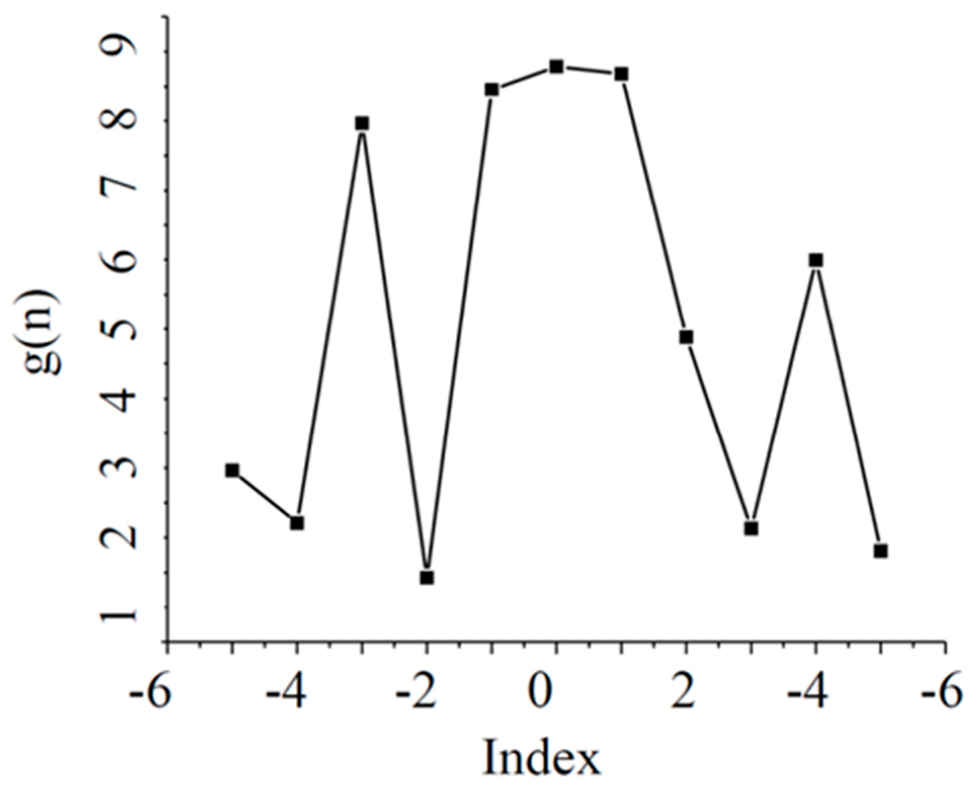
After optimization by genetic algorithm, the value of g(n) are shown in Figure 2. All the optimized parameters are within the established threshold range.
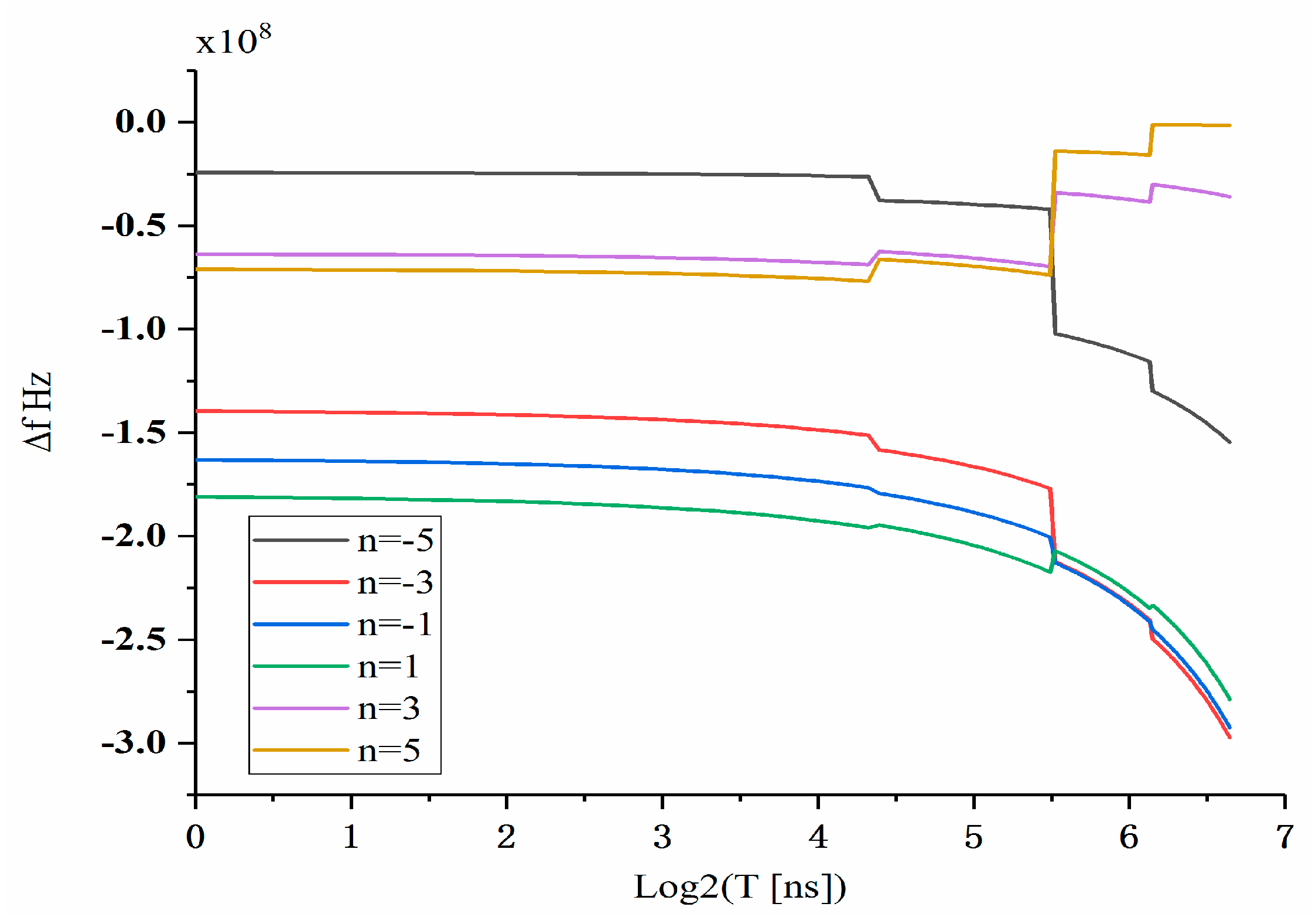
The frequency offset of the optimized array elements is shown in Figure 3. To show the large variations of different array elements, the x-axis representing time is in logarithmic scale. Figure 3 shows that the optimized shift frequency Δf completely satisfies the range −0.3–0 GHz.
The frequency variation behavior shown in the figure illustrates that the frequency of each array element has incurred three frequency changes in a total of four curve segments. Each curve represents a focal point, and the result is consistent with the sequential focus at four points.
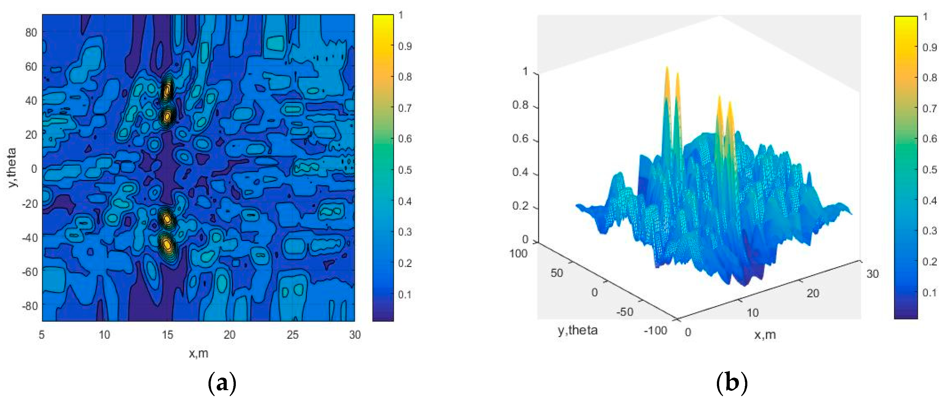
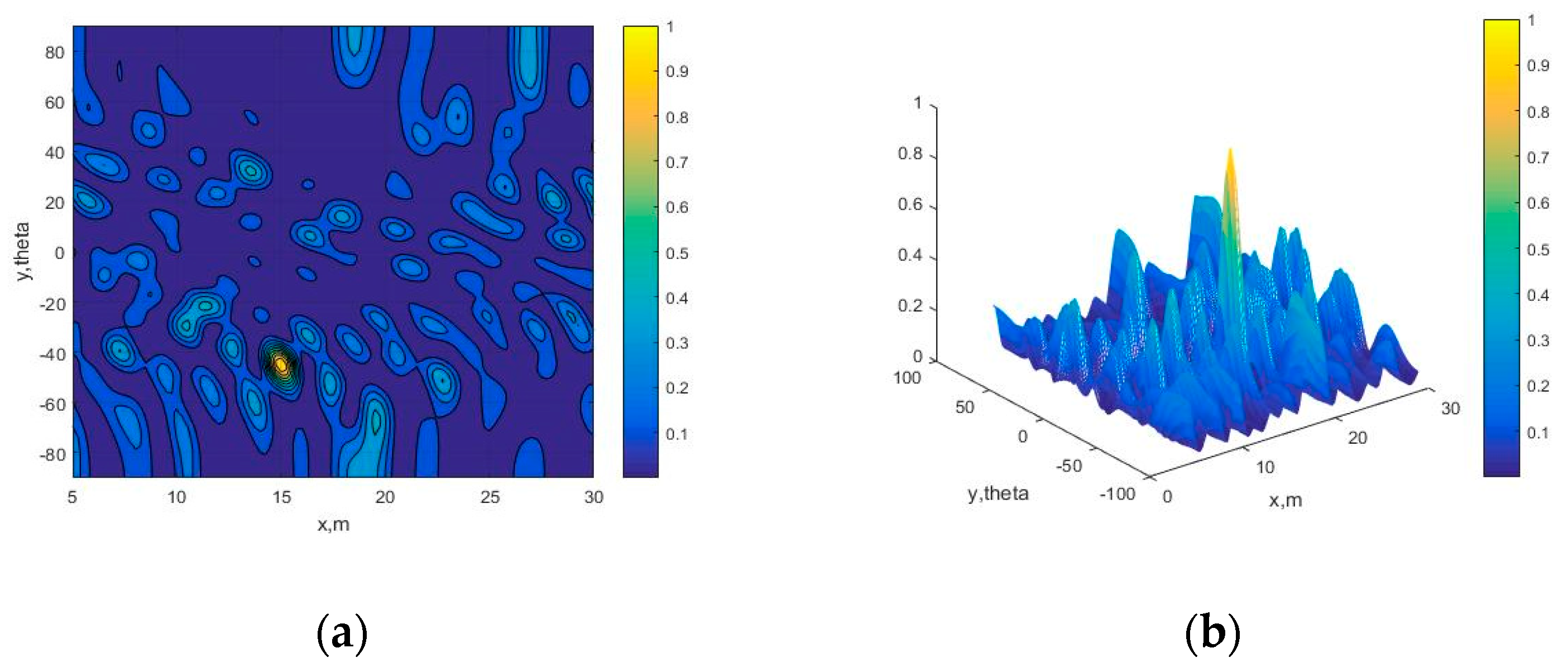
Figure 4 is a schematic structural diagram of an actual simulation signal for sequential focus at multiple points. The simulation results are shown in Figure 5 and Figure 6. As time increases, the focus position has sequentially shifted from the first point to the last point, and the focal spot size does not change significantly. This proves that the frequency is controlled successfully through different time periods and that sequential focus at the four target points is achieved.
We now show the focal spot parameter values at specific times, with the data shown in Table 2.
4. Conclusions
In summary, this paper develops a method for multi-point sequential focusing and multi-point simultaneous focusing in the far-field. The first section introduces four-point sequential focusing, and the optimized target function for four-point sequential focusing is given. On the basis of the previous single-point focusing, sequential focus at the four points is achieved by controlling the time period. Then, the validity of the focal point is examined. A reasonable threshold range of the four points is then found by calculating the threshold range of the four points and by finding the intersection set. Finally, sequential focusing of the four points is validated through simulation. The so-called multi-point sequential focusing is really an extension of single-point focusing. By controlling the frequency in different time intervals with functions, in-phase addition of a single point in space is achieved.
Author Contributions
Conceptualization, S.D. and H.T.; investigation, Y.-M.H.; writing—original draft preparation, S.D. and Y.-M.H.; writing—review and editing B.-Z.W. and M.B.
Funding
This research was funded by National Natural Science Foundation of China, Grant No. 61601087; Sichuan Science and Technology Program, grant number 2018GZ0518.
Conflicts of Interest
The authors declare no conflict of interest.
References
- Antonik, P.; Wicks, M.C.; Griffiths, H.D.; Baker, C.J. Frequency diverse array radars. In Proceedings of the IEEE Radar Conference, Verona, NY, USA, 24–27 April 2006; pp. 215–217. [Google Scholar]
- Antonik, P.; Wicks, M.C.; Griffiths, H.D.; Baker, C.J. Range dependent beam using element level waveform diversity. In Proceedings of the International Waveform Diversity and Design Conference, Lihue, HI, USA, 22–27 January 2006; pp. 1–4. [Google Scholar]
- Wicks, M.C.; Antonik, P. Frequency Diverse Array with Independent Modulation of Frequency, Amplitude, and Phase. International Patent Application No. 7319427, 15 January 2008. [Google Scholar]
- Wicks, M.C.; Antonik, P. Method and Apparatus for a Frequency Diverse Array, Amplitude. U.S. Patent 7, 31 March 2008. [Google Scholar]
- Huang, J.; Tong, K.F.; Baker, J. Frequency diverse array with beam scanning feather. In Proceedings of the IEEE International Symposium on Antennas and Propagation, San Diego, CA, USA, 5–11 July 2008; pp. 2324–2327. [Google Scholar]
- Higgins, T.; Blunt, S.D. Analysis of rang-angle coupled beam-forming with frequency-diverse chirps. In Proceedings of the International Waveform Diversity and Design Conference, Kissimmee, FL, USA, 8–13 February 2009; pp. 140–144. [Google Scholar]
- Jones, A.M.; Rigling, B.D. Planar frequency diverse array receiver architechre. In Proceedings of the IEEE Radar conference, Atlanta, GA, USA, 7–11 May 2012; pp. 226–229. [Google Scholar]
- Shin, J.; Choi, J.H.; Kim, J.; Yang, J.; Lee, W.; Cheon, C. Full-wave simulation of requency diverse array antenna using FDTD method. In Proceedings of the Asia-Pacific Microwave Conference, Seoul, Korea, 5–8 November 2013; pp. 1070–1072. [Google Scholar]
- Secmen, M.; Demir, S.; Hizal, A.; Eker, T. Frequency diverse array antenna with periodic time modulated pattern in range and angle. In Proceedings of the IEEE Radar Conference, Boston, MA, USA, 17–20 April 2007; pp. 427–430. [Google Scholar]
- Eker, T.; Demir, S.; Hizal, A. Exploitation of linear frequency modulation continuous waveform (LFMCW) for frequency diverse arrays. IEEE Trans. Antennas Propag. 2013, 61, 3546–3553. [Google Scholar] [CrossRef]
- Cetinepe, T.; Demir, S. Multipath characteristics of frequency diverse arrays over a ground plane. IEEE Trans. Antennas Propag. 2014, 62, 3567–3574. [Google Scholar] [CrossRef]
- Khan, W.; Qureshi, I.M.; Saeed, S. Frequency Diverse Array Radar with Logarithmically Increasing Frequency Offset. IEEE Antennas Wirel. Propag. Lett. 2015, 14, 499–502. [Google Scholar] [CrossRef]
- Han, S.; Fan, C.; Huang, X. Frequency diverse array with time-dependent transmit weights. In Proceedings of the IEEE 13th International Conference on Signal Processing (ICSP), Chengdu, China, 6–10 November 2016; pp. 448–451. [Google Scholar]
- Yao, A.M.; Rocca, P.; Wu, W.; Massa, A.; Fang, D.G. Synthesis of Time-Modulated Frequency Diverse Arrays for Short-Range Multi-Focusing. IEEE J. Sel. Top. Signal Process. 2017, 11, 282–294. [Google Scholar] [CrossRef]
- Yao, A.M.; Wu, W.; Fang, D.G. Frequency diverse array antenna using time-modulated optimized frequency offset to obtain timeinvariant spatial fine focusing beampattern. IEEE Trans. Antennas Propag. 2016, 64, 4434–4446. [Google Scholar] [CrossRef]
- Yao, A.M.; Wu, W.; Fang, D.G. Solutions of Time-Invariant Spatial Focusing for Multi-Targets Using Time Modulated Frequency Diverse Antenna Arrays. IEEE Trans. Antennas Propag. 2017, 65, 552–566. [Google Scholar] [CrossRef]
- Fang, D.G.; Yao, A.M.; Wu, W. Synthesis of 4-D beampatterns using 4-D arrays. In Proceedings of the 2016 IEEE International Symposium on Antennas and Propagation (APSURSI), Fajardo, Puerto Rico, 26 June–1 July 2016; pp. 703–704. [Google Scholar]
- Yang, Y.; Wang, H.; Gu, S. Optimization of Multi-Carrier Frequency Diverse Array for Wireless Power Transmission. In Proceedings of the 2018 Asia-Pacific Microwave Conference (APMC), Kyoto, Japan, 6–9 November 2018; pp. 43–45. [Google Scholar]
Figure 1.
The schematic of frequency diversity array.

Figure 2.
The value of g(n).

Figure 3.
Frequency offset of array element.

Figure 4.
Signals fed in the array elements.
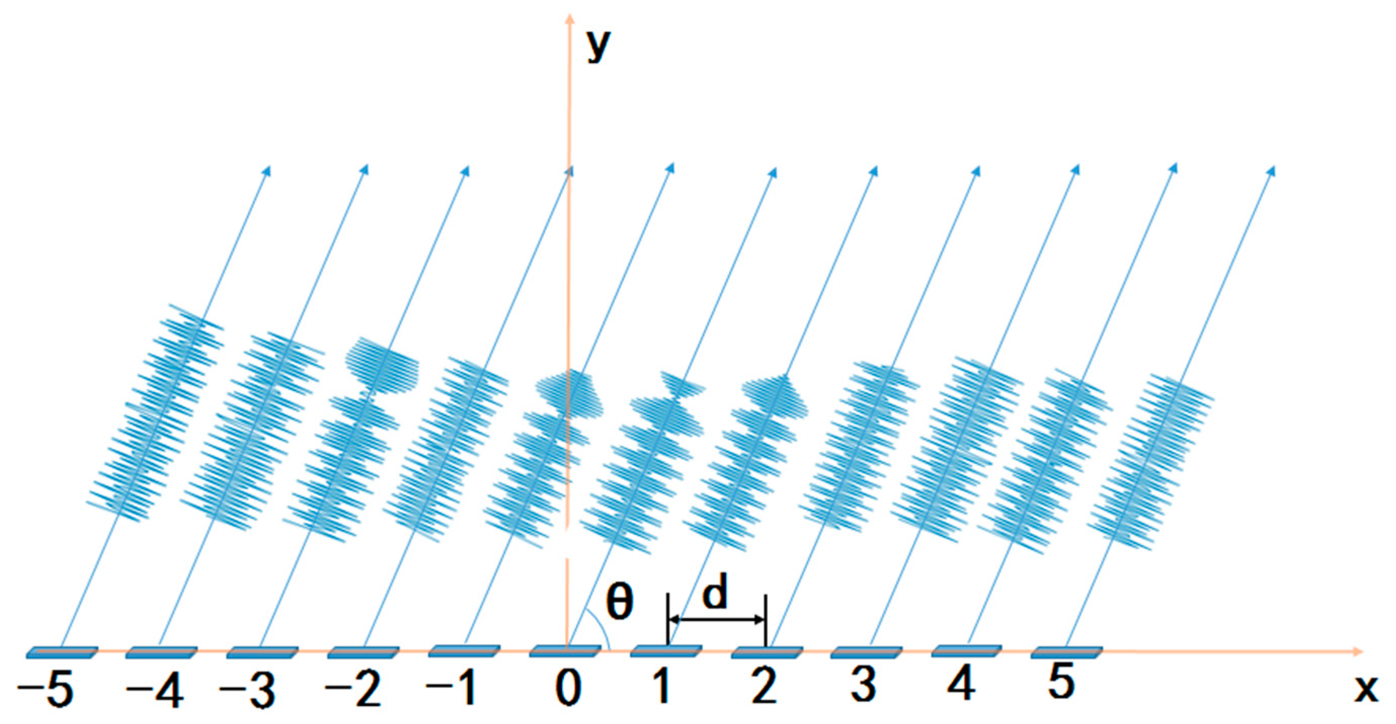
Figure 5.
Multi-point sequential focus: (a) top view of focus at t = 0 ns; (b) side view of focus at t = 0 ns; (c) top view of focus at t = 5 ns; (d) side view of focus at t = 5 ns; (e) top view of focus at t = 10 ns; (f) side view of focus at t = 10 ns; (g) top view of focus at t = 15 ns; (h) side view of focus at t = 15 ns.


Figure 6.
Focusing position. (a) Total field diagram for four-point sequential focus; (b) perspective view of four-point sequential focus.
Figure 6.
Focusing position. (a) Total field diagram for four-point sequential focus; (b) perspective view of four-point sequential focus.

Table 1.
Range of multi-point sequential focus frequency offset function parameter g(n).
| Index | Upper Limited | Lower Limited |
|---|---|---|
| −5 | 1.7678 | 7.4090 |
| −4 | 1.4142 | 7.7272 |
| −3 | 1.0607 | 8.0454 |
| −2 | 0.7071 | 8.3636 |
| −1 | 0.3536 | 8.6818 |
| 0 | 0 | 9 |
| 1 | 0.3536 | 8.6818 |
| 2 | 0.7071 | 8.3636 |
| 3 | 1.0607 | 8.0454 |
| 4 | 1.4142 | 7.7272 |
| 5 | 1.7678 | 7.4090 |
| −5 | 1.7678 | 7.4090 |
| −4 | 1.4142 | 7.7272 |
| −3 | 1.0607 | 8.0454 |
| −2 | 0.7071 | 8.3636 |
Table 2.
Values of the parameters.
| Time | Half-Power Angular Width (°) | Half-Power Distance width (m) |
|---|---|---|
| 0 | 13.9612 | 1.4851 |
| 5 ns | 11.4681 | 1.4851 |
| 10 ns | 11.4681 | 1.4851 |
| 15 ns | 13.9612 | 0.9901 |
| 20 ns | 13.9612 | 0.9901 |
© 2019 by the authors. Licensee MDPI, Basel, Switzerland. This article is an open access article distributed under the terms and conditions of the Creative Commons Attribution (CC BY) license (http://creativecommons.org/licenses/by/4.0/).
Share and Cite
MDPI and ACS Style
Ding, S.; Huang, Y.-M.; Tang, H.; Bozzi, M.; Wang, B.-Z. Achieving Spatial Multi-Point Focusing by Frequency Diversity Array. Electronics 2019, 8, 883. https://doi.org/10.3390/electronics8080883
AMA Style
Ding S, Huang Y-M, Tang H, Bozzi M, Wang B-Z. Achieving Spatial Multi-Point Focusing by Frequency Diversity Array. Electronics. 2019; 8(8):883. https://doi.org/10.3390/electronics8080883
Chicago/Turabian StyleDing, Shuai, Yong-Mao Huang, Huan Tang, Maurizio Bozzi, and Bing-Zhong Wang. 2019. "Achieving Spatial Multi-Point Focusing by Frequency Diversity Array" Electronics 8, no. 8: 883. https://doi.org/10.3390/electronics8080883
Note that from the first issue of 2016, this journal uses article numbers instead of page numbers. See further details here.