Support-Vector-Regression-Based Kinematics Solution and Finite-Time Tracking Control Framework for Uncertain Gough–Stewart Platform

Abstract

This paper addresses the trajectory tracking control problem of a six-degree-of-freedom Gough–Stewart Platform (GSP) by proposing a control strategy that combines a sliding mode (SM) controller with a rapid forward kinematics solution algorithm. The study first develops an efficient forward kinematics method that integrates Support Vector Regression (SVR) with the Levenberg–Marquardt algorithm, effectively resolving issues related to multiple solutions and local optima encountered in traditional iterative approaches. Subsequently, a SM controller based on the GSP’s dynamic model is designed to achieve high-precision trajectory tracking. The proposed control strategy’s robustness and effectiveness are validated through simulation experiments, demonstrating superior performance in the presence of model discrepancies and external disturbances. Comparative analysis with traditional PD controllers and linear SM controllers shows that the proposed method offers significant advantages in both tracking accuracy and control response speed. This research provides a novel solution for high-precision control in GSP applications.

1. Introduction

The Gough–Stewart Platform (GSP) [1,2,3], a six-degree-of-freedom parallel mechanism first introduced in 1965 as a flight simulator, is renowned for its high-speed performance, dynamic stability, and precise repeatability. Its advanced parallel structure has established its indispensability across various applications. In aircraft simulation, it ensures precision and stability. For vibration isolation systems, it provides a critical dynamic response. In surgical robotics, it offers exceptional accuracy, and in high-precision machining, it ensures consistent performance across varying conditions.

The control of parallel mechanisms [1,4,5] like the GSP presents significant challenges, primarily due to the strong coupling and nonlinear characteristics inherent in their control variables. These complexities have made the control of the GSP a central topic of interest within the academic community, driving ongoing research efforts aimed at developing more effective control strategies. One of the fundamental objectives in controlling the GSP is to ensure high-precision tracking of predefined trajectories, a task that becomes particularly challenging when the system is subject to external disturbances. Furthermore, in nonlinear systems with strict-feedback forms, preassigned finite-time control schemes have been developed to guarantee rapid convergence and ensure that all signals of the closed-loop system meet preassigned finite-time stability criteria [6], which could also inform GSP control strategies that demand fast and precise trajectory tracking.

The mainstream control methods for GSP can be categorized into task-space and joint-space control. Task-space control involves using sensors to obtain the end-effector’s position and orientation, followed by feedback control. However, the high cost and spatial requirements of these sensors limit its practical application. In contrast, joint-space control directly adjusts the lengths of the GSP’s six legs to track the desired trajectory. A key challenge in joint-space control is the requirement to rapidly compute the end-effector’s position and orientation from the leg lengths. This forward kinematics computation is essential to ensure that the control system accurately correlates the actuator inputs (leg lengths) with the resulting platform motion, which is necessary to meet real-time demands and maintain precise trajectory tracking.

Solving the forward kinematics of GSP is particularly challenging due to the complex nonlinear coupled equations involved. Researchers have developed various methods including algebraic elimination, interval analysis, and optimization techniques to address this problem. In [7], a 20th-degree univariate polynomial for a general 6-6 Stewart platform was derived using a 15 × 15 Sylvester matrix. Reference [8] proposed a hybrid method combining the immune algorithm, genetic algorithm, and fuzzy system to solve the forward kinematics problem of the Stewart platform, comparing it with the standard genetic algorithm. Reference [9] proposed a method for real-time forward kinematics of Stewart platforms, which involves decomposing the leg space into cells, using inverse kinematics to generate data, and storing model parameters in a lookup table for fast online computation. Similarly, reference [10] proposed an efficient algorithm based on dual quaternions and the Jacobian matrix, converting the problem into a system of quadratic equations and developing a convergent iterative solution. The use of sensor feedback is also a common approach for solving the forward kinematics of parallel platforms. In [11], a method using tetrahedron configurations is proposed to solve the forward kinematics of the 6-6 Stewart platform, avoiding numerical iteration and providing a unique solution, which makes it suitable for real-time applications.

However, iterative methods still have limitations, such as issues with multiple solutions and local optima. To address these challenges, some researchers have recently turned to neural network algorithms to enhance the accuracy of the solutions. In [12], a forward kinematic solution for the Stewart platform was developed by employing a linear estimator based on Luenberger’s observer, alongside a nonlinear estimator utilizing a measurement model. Given the complexity of designing the estimator parameters, a neural network with a multi-layer perceptron architecture was introduced to optimize the estimation gain via backpropagation. The proposed methodology was validated through simulations, demonstrating its robustness and accuracy. In [13], a soft-computing-based approach is introduced to solve the forward kinematics problem of the Stewart platform. A multi-layer feed-forward neural network is trained using different metaheuristic optimizers, including Particle Swarm Optimization (PSO), Modified Chaotic Invasive Weed Optimization (MCIWO), and Teachers’ Learning-Based Optimization (TLBO), with the training dataset generated from the inverse kinematics solution.

Despite these advances, there is still no universally effective method for real-time solutions to the forward kinematics of parallel mechanisms. To further enhance these approaches, this paper proposes a hybrid method that combines SVR with iterative solving. First, the system of nonlinear equations for the forward kinematics is formulated, and data generated via inverse kinematics is used to train the SVR model. The SVR then provides an initial guess for the iterative process, which is refined using the Levenberg–Marquardt method. Compared to neural networks, SVR models are more compact and can produce results faster, making them more suitable for real-time applications.

Accurate and fast forward kinematics solutions are not only essential for determining the platform’s position and orientation but are also crucial for implementing advanced control strategies. Advanced control strategies for the GSP aim to achieve precise trajectory tracking and robust disturbance rejection. Traditional methods [14], such as PID [15] and fuzzy control [16], have been applied with some success, but they often lack the necessary tracking speed and accuracy, keeping GSP control an active research area. In [17], an improved equivalent input disturbance (IEID) method combined with SM control was proposed to enhance trajectory tracking and disturbance rejection. A joint space neural network compensation method was introduced in [18] to address uncertain loads in Stewart robots. A decentralized adaptive synchronized control scheme was presented in [4], which integrates synchronization and model reference adaptive control (MRAC) to ensure tracking accuracy and joint coordination under uncertainties. The method features a simple structure and does not rely on precise dynamic models, making it suitable for real-time control. Additionally, reference [19] integrated a dynamic model of hydraulic cylinders with a SM controller to achieve trajectory tracking in hydraulically actuated GSPs.

Most existing schemes operate in joint space, which limits their effectiveness in handling the nonlinearities and external disturbances inherent to the GSP. To address these challenges, accurate dynamic modeling has become essential. Several approaches have been developed for the dynamic modeling of the GSP, including the principle of virtual work [20], screw theory [21], the Lagrange method [22], and the Newton–Euler method [23]. The results obtained from these methods for solving the dynamic equations of the GSP are generally similar. Current research in this area focuses on improving computation speed and reducing the number of parameters, which is critical for enabling real-time control. In parallel, advanced control strategies, such as direct adaptive finite-time control using neural networks, have been proposed to address additional challenges such as time delays and quantized inputs in strict-feedback nonlinear systems, offering a novel approach to further improve the control performance of systems like the GSP [24].

When addressing external disturbances and ensuring stability in complex systems, the application of sliding mode control (SMC) has proven to be effective. For example, a pre-assigned time sliding mode approach has been proposed for distributed secondary control in microgrids, where a time-varying gain function is used to set the convergence time independently of initial conditions and other design parameters [25]. This ensures that system states, such as frequency and voltage errors, converge to the sliding surface within the pre-assigned time, making it a robust method for managing systems under external disturbances and uncertainties. Building on this concept, recent studies have extended the use of SMC to multi-system synchronization problems, particularly under uncertainties and disturbances. For instance, the finite-time synchronization of uncertain chaotic systems using SMC [26] provides a solid foundation for applying similar control strategies to systems like the Stewart platform, where precise coordination and disturbance rejection are critical. Furthermore, to further enhance the system’s robustness against disturbances, event-triggered control methods have also been successfully employed. A notable example is the improved event-triggered-based anti-disturbance control method proposed for Takagi–Sugeno fuzzy wind-turbine systems [27], which offers valuable insights for optimizing control strategies in systems like the Stewart platform. Additionally, in addressing motion and input constraints in spacecraft operations, a learning-based robust optimal control approach has been proposed, demonstrating how robust control strategies can be applied to systems facing similar challenges as the Stewart platform [28].

SM control [29,30] is considered a robust control technique for complex higher-order nonlinear systems, particularly under the influence of parametric uncertainties [31] and external disturbances. Given its robustness and effectiveness in handling uncertainties, SMC [32] has been widely adopted in various robotic systems. In [17], an integrated control method combining an improved equivalent-input-disturbance (IEID) estimator and sliding-mode control (SMC) [33] is proposed for the Stewart platform, aimed at enhancing reference tracking and disturbance rejection. A state observer and IEID estimator are used to compensate for overall disturbances, while a small sliding-mode gain reduces chattering and ensures tracking precision. The system’s stability is analyzed based on Lyapunov theory, with the observer and estimator gains designed using a linear matrix inequality. The experimental results demonstrate superior disturbance rejection compared to standalone SMC and IEID methods. In [34], a multivariable integral SM controller is proposed for MIMO systems, where the conventional discontinuous feedback control is replaced by a multivariable super twisting algorithm to eliminate chattering while maintaining disturbance rejection. The proposed controller achieves continuous control and demonstrates effectiveness through simulation results. In [35], a fast terminal SM control technique is proposed for robust tracking of a nonlinear mass–spring system with parametric uncertainties and external disturbances. The method uses Lyapunov stability theory [36] and is validated through simulations and experiments. In [37], a novel non-singular terminal SM surface incorporating an arctan function is proposed for trajectory tracking of n-link robotic manipulators. The effectiveness of the approach is demonstrated using a two-link robotic manipulator.

The main contributions of this paper can be divided into three parts:

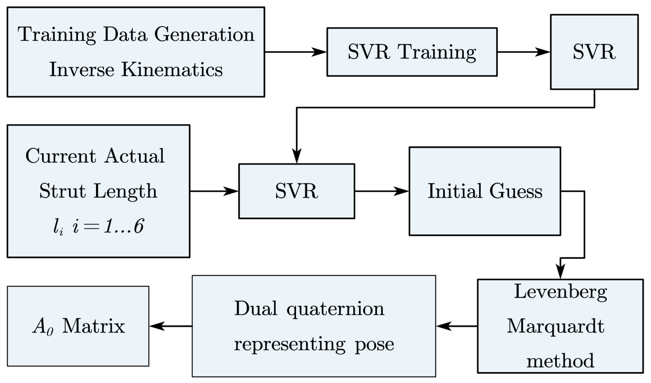
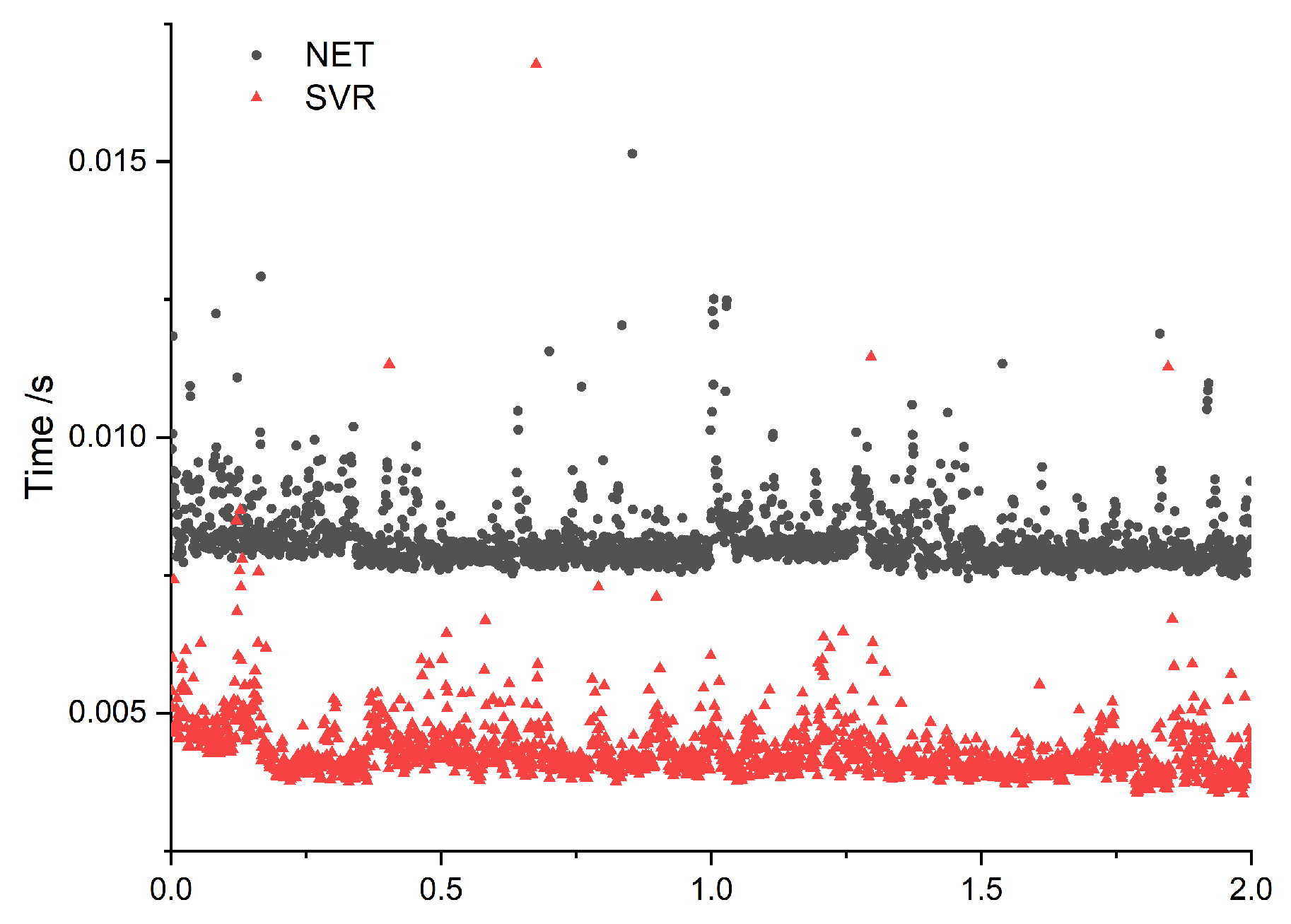
• Novel Kinematics Solution Based on SVR: This paper proposes an innovative kinematics solution for Generalized Spatial Mechanisms (GSP) by integrating Support Vector Regression (SVR) with the Levenberg–Marquardt method. Unlike traditional iterative algorithms, this hybrid approach ensures computational accuracy through iteration while leveraging SVR for efficient inference of the initial iterative values. This not only prevents the iteration from getting trapped in local optima but also improves overall computational efficiency. The proposed method accelerates convergence and reduces sensitivity to initial conditions, making it a highly effective alternative for solving complex spatial mechanism problems.
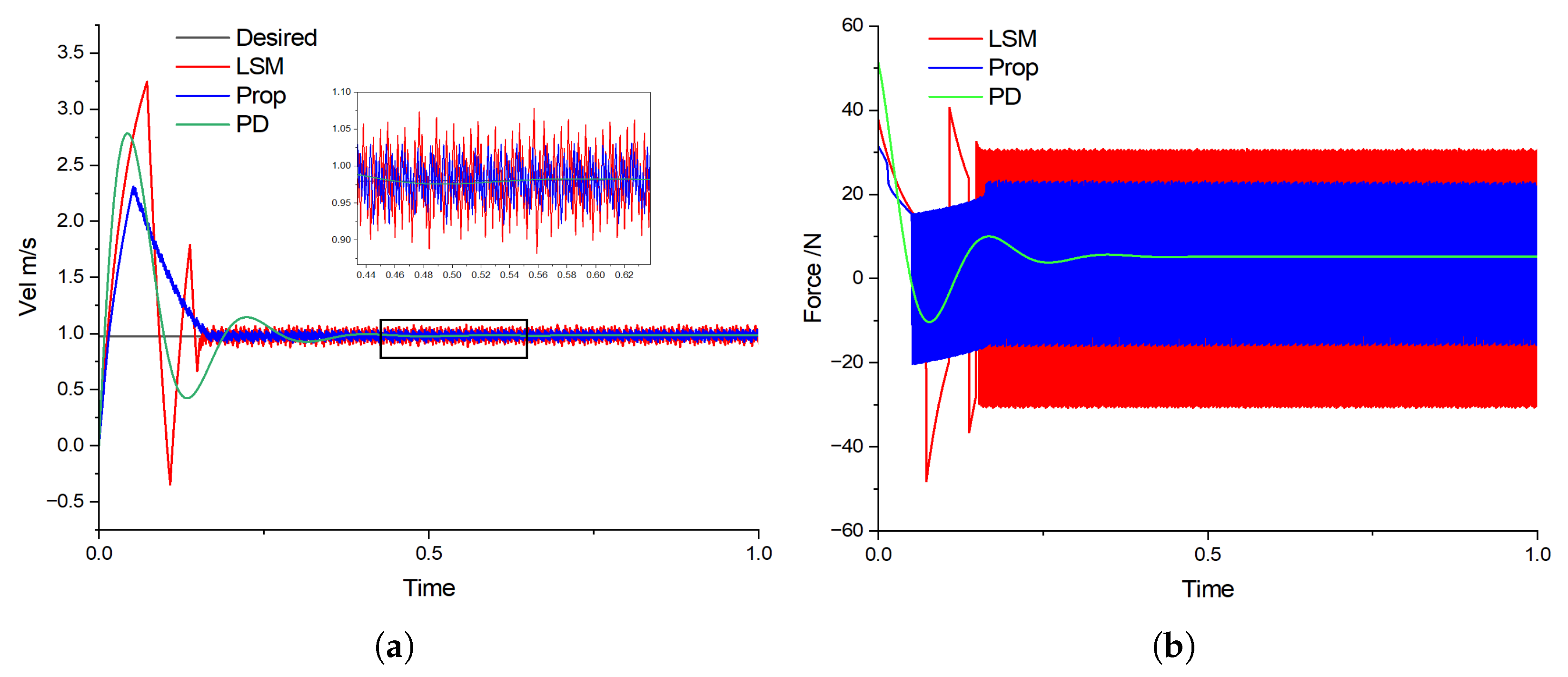
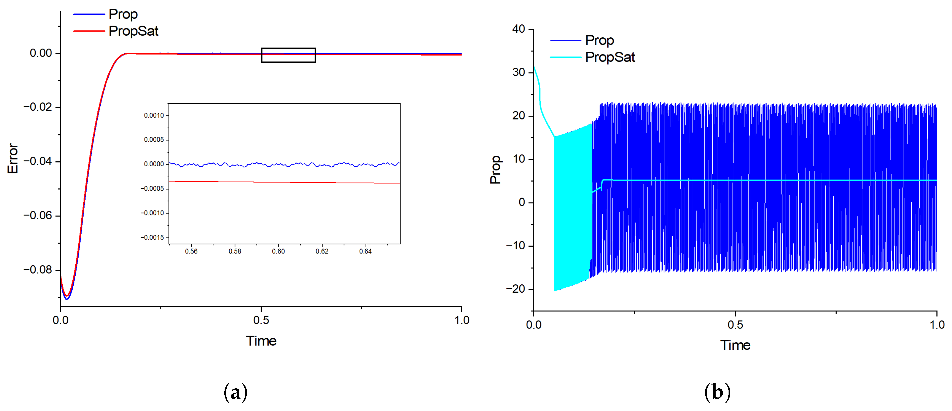
• Finite-Time Convergent Precise Trajectory Tracking: A significant advancement of this study is the introduction of a finite-time convergent sliding mode control (SMC) strategy, specifically designed for the precise and rapid trajectory tracking of Generalized Spatial Mechanisms (GSP). Compared to traditional SMC methods, the proposed approach guarantees finite-time convergence, ensuring deterministic control performance within a predefined time horizon. Furthermore, in comparison with the widely used PID control method, this approach exhibits smaller tracking errors and faster convergence speed, making it particularly suitable for scenarios that demand high responsiveness and control precision.
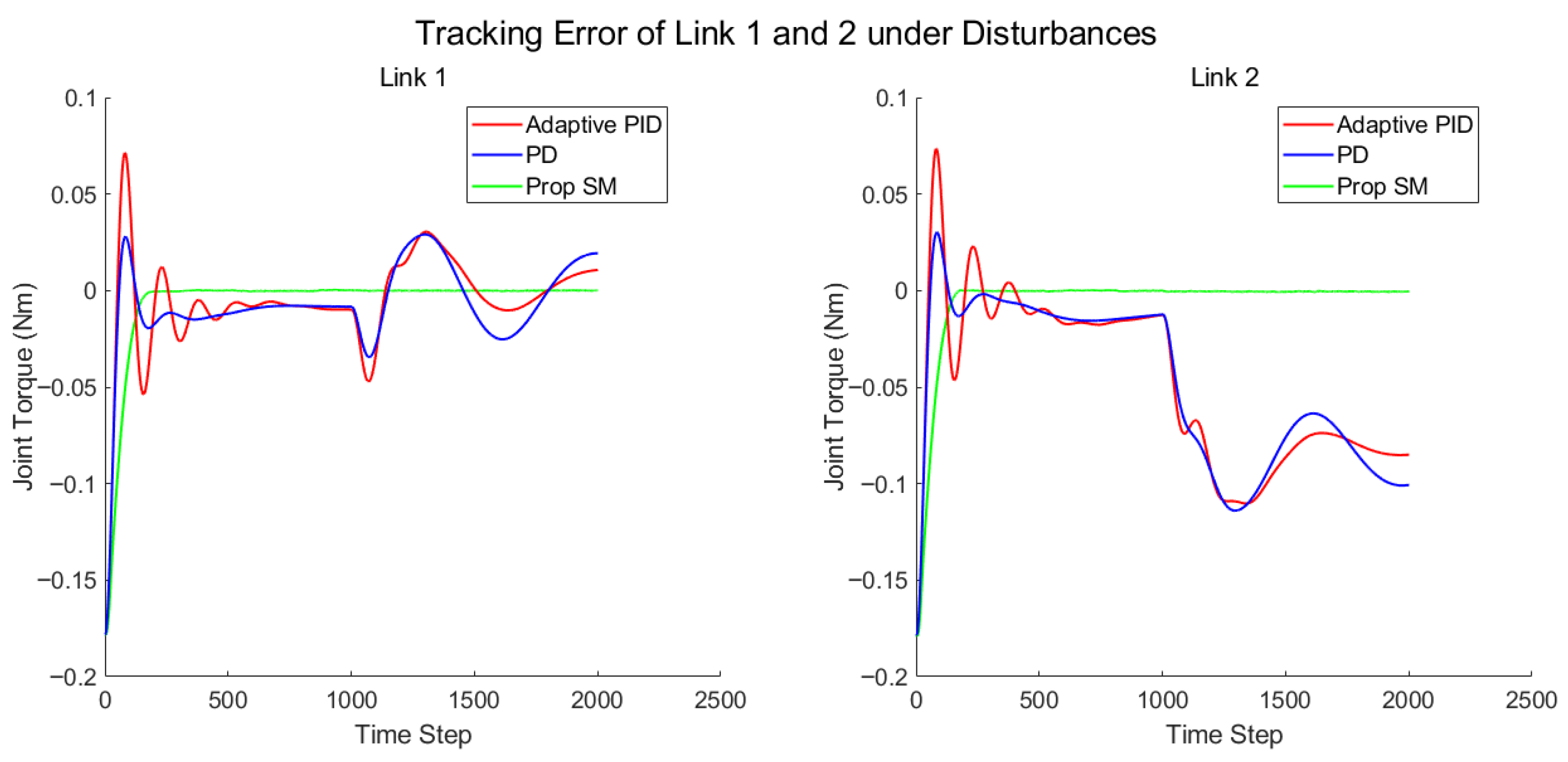
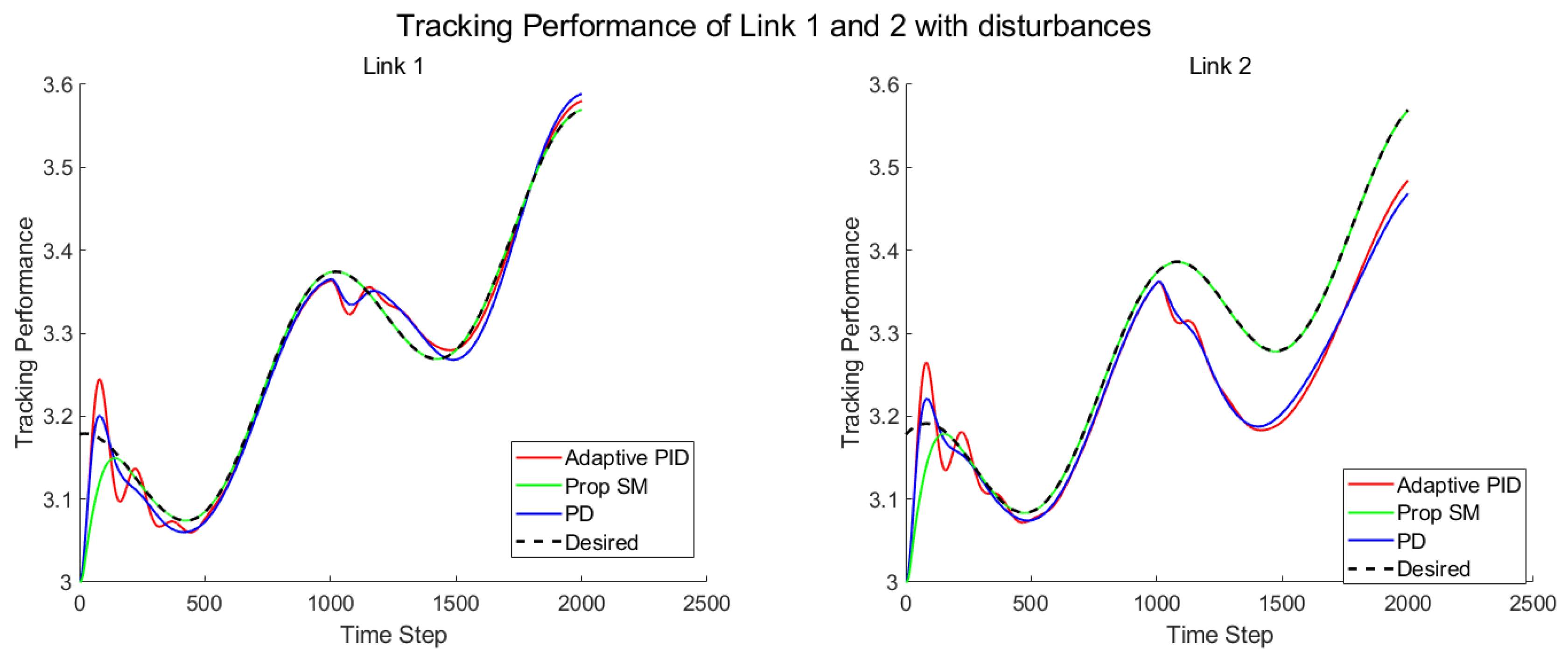
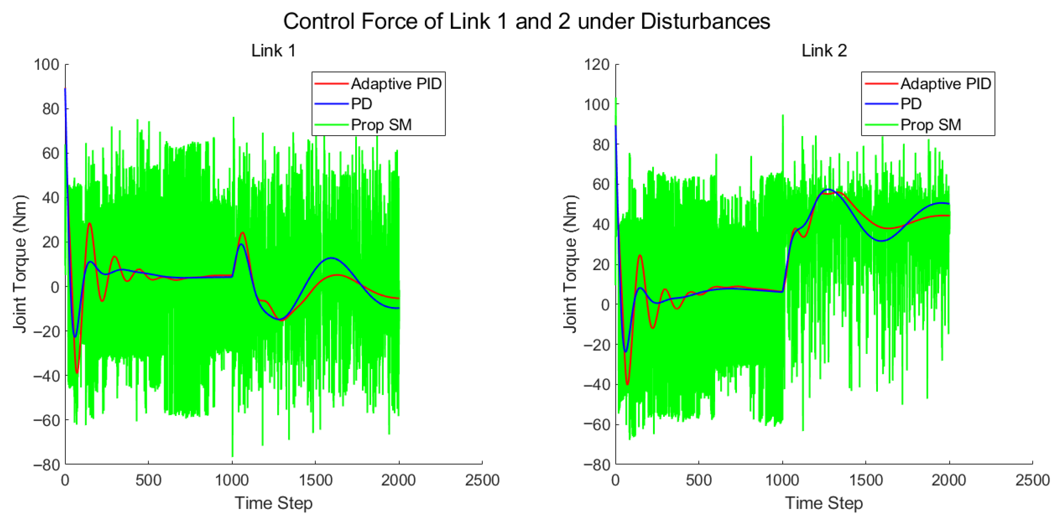
• Enhanced Robustness Against Uncertainties and Disturbances: The proposed control framework explicitly considers model uncertainties and external disturbances, thereby significantly enhancing system robustness. Unlike conventional control schemes, which often suffer from degraded performance under varying conditions, our method ensures sustained precision and stability. Extensive simulations validate the effectiveness of our approach, achieving superior tracking performance and robustness even when subject to unknown disturbances and model mismatches.

This paper is structured into five sections. Section 1 introduces the research background and current state of the GSP. Section 2 outlines the control problems that need to be addressed. In Section 3, a model-based SM controller is proposed, along with a forward kinematics solution method that combines an SVR machine with an iterative algorithm, and the stability of the controller is demonstrated. Section 4 presents the simulation results, including a comparison with PD control, Adaptive PID control, and linear SM control. Finally, Section 5 provides a summary and conclusion of the entire paper.

2. Problem Statement

In this section, we define the basic structure and control problem of the GSP. Figure 1a illustrates a 6-degree-of-freedom Stewart platform. The platform consists of a fixed base, a movable platform, and six identical legs connecting the movable platform to the fixed base. Each linkage is connected to the fixed base and the movable platform through a universal joint at one end and a spherical joint at the other. The length of each linkage can be adjusted via hydraulic or screw-based actuators, allowing the movable platform to achieve effective 6-degree-of-freedom motion.

Define the coordinate system of the fixed platform as the base coordinate system $\mathbf{B}$ and the coordinate system fixed to the upper platform as the moving coordinate system $\mathbf{T}$, as shown in Figure 1b. The origins of the two coordinate systems are located at the centroids of the movable and fixed platforms, respectively. At the initial position, the $x_T{y}_T$ plane is parallel to the horizontal plane. $z_T$ and z are perpendicular to the horizontal plane. The coordinates ${\mathbf{a}}_{\mathbf{i}}$ and ${\mathbf{b}}_{\mathbf{i}}$ ($i=1\dots 6$) represent the position vectors of the upper and lower joints connecting the legs to the fixed and movable platforms, respectively. According to this definition, ${}^B\mathbf{a}_{\mathbf{i}}$ represents the position vector of the universal joint relative to the $\mathbf{B}$ coordinate system, and ${}^T\mathbf{b}_{\mathbf{i}}$ represents the position vector of the spherical joint relative to the $\mathbf{T}$ coordinate system. Therefore, both vectors are constants determined by the configuration. Define the vector $\mathbf{P}={\left(p_x,p_y,p_z\right)}^T$ as the position of the origin of the moving coordinate system $\mathbf{T}$ relative to the base coordinate system $\mathbf{B}$. The vector ${\mathbf{l}}_{\mathbf{i}}$ represents the linkage vector connecting joints ${\mathbf{a}}_{\mathbf{i}}$ and ${\mathbf{b}}_{\mathbf{i}}$, and ${\mathbf{r}}_{\mathbf{i}}$ is the length of the linkage.

The dynamics of the Stewart–Gough Platform can be expressed as

$$\mathbf{A}\left(\mathbf{r}\right)\ddot{\mathbf{r}}+\mathbf{B}(\mathbf{r},\dot{\mathbf{r}})\dot{\mathbf{r}}+\mathbf{C}\left(\mathbf{r}\right)=\mathbf{f}+\mathbf{\tau }$$

(1)

where $\mathbf{r}={\left(r_1,r_2,\dots ,r_6\right)}^T$ represents the vector of leg lengths, $\mathbf{f}={\left(f_1,f_2,\dots ,f_6\right)}^T$ represents the vector of forces applied along the legs, and $\mathbf{\tau }={\left({\tau }_1,{\tau }_2,\dots ,{\tau }_6\right)}^T$ represents the vector of forces exerted on the links due to external disturbances. The matrix $\mathbf{A}\left(\mathbf{r}\right)$, a 6 × 6 matrix, represents the inertia matrix, which characterizes the mass distribution and resistance to acceleration within the system. The matrix $\mathbf{B}(\mathbf{r},\dot{\mathbf{r}})$, also a 6 × 6 matrix, captures the Coriolis and centrifugal forces that arise due to the system’s motion. Lastly, $\mathbf{C}\left(\mathbf{r}\right)$ is a 6 × 1 vector representing the gravitational forces acting on the system based on its current configuration.

Considering that there are discrepancies between the established dynamic model and the actual model,

$$\begin{array}{cc}\hfill \mathbf{A}\left(\mathbf{r}\right)& ={\mathbf{A}}_{\mathbf{0}}\left(\mathbf{r}\right)+\Delta \mathbf{A}\left(\mathbf{r}\right)\hfill \end{array}$$

(2)

$$\begin{array}{cc}\hfill \mathbf{B}\left(\mathbf{r},\dot{\mathbf{r}}\right)& ={\mathbf{B}}_{\mathbf{0}}\left(\mathbf{r},\dot{\mathbf{r}}\right)+\Delta \mathbf{B}\left(\mathbf{r},\dot{\mathbf{r}}\right)\hfill \end{array}$$

(3)

$$\begin{array}{cc}\hfill \mathbf{C}\left(\mathbf{r}\right)& ={\mathbf{C}}_{\mathbf{0}}\left(\mathbf{r}\right)+\Delta \mathbf{C}\left(\mathbf{r}\right)\hfill \end{array}$$

(4)

The matrices ${\mathbf{A}}_{\mathbf{0}}\left(\mathbf{r}\right)$, ${\mathbf{B}}_{\mathbf{0}}(\mathbf{r},\dot{\mathbf{r}})$, and ${\mathbf{C}}_{\mathbf{0}}\left(\mathbf{r}\right)$ represent the parameter matrices obtained through the dynamic model, while $\Delta \mathbf{A}\left(\mathbf{r}\right)$, $\Delta \mathbf{B}(\mathbf{r},\dot{\mathbf{r}})$, and $\Delta \mathbf{C}\left(\mathbf{r}\right)$ represent the uncertainties of the system model. The link tracking error ${\mathbf{e}}_{\mathbf{1}}$ and its derivative ${\mathbf{e}}_{\mathbf{2}}$ are defined as follows:

$$\begin{array}{cc}\hfill {\mathbf{e}}_{\mathbf{1}}& =\mathbf{r}-{\mathbf{r}}_{\mathbf{g}}\hfill \end{array}$$

(5)

$$\begin{array}{cc}\hfill {\mathbf{e}}_{\mathbf{2}}& ={\displaystyle \frac{d}{dt}}{\mathbf{e}}_{\mathbf{1}}=\dot{\mathbf{r}}-{\dot{\mathbf{r}}}_g\hfill \end{array}$$

(6)

where $r_g$ represents the vector of desired link lengths, and ${\dot{r}}_g$ represents the desired velocity, both of which are 6-dimensional vectors. Similarly, r denotes the current actual link lengths, and $\dot{r}$ represents the actual link velocities, both also being 6-dimensional vectors. The error between the actual and desired values is denoted by ${\mathbf{e}}_{\mathbf{1}}$, which is a 6-dimensional vector, while ${\mathbf{e}}_{\mathbf{2}}$ represents the time derivative of ${\mathbf{e}}_{\mathbf{1}}$ and is likewise a 6-dimensional vector. After simplification, we obtain

$$\begin{array}{cc}\dot{{\mathbf{e}}_{\mathbf{1}}}\hfill & ={\mathbf{e}}_{\mathbf{2}}\hfill \end{array}$$

(7)

$$\begin{array}{cc}\hfill \dot{{\mathbf{e}}_{\mathbf{2}}}& =\mathbf{G}\left(\mathbf{e}\right)+{\mathbf{A}}_0^{-1}\left(\mathbf{r}\right)\mathbf{f}+\mathbf{D}(\mathbf{e},\dot{\mathbf{e}})\hfill \end{array}$$

(8)

where $\mathbf{e}={\left[{{\mathbf{e}}_{\mathbf{1}}}^T,{{\mathbf{e}}_{\mathbf{2}}}^T\right]}^T\in {\mathbb{R}}^{12}$. $\mathbf{G}\left(\mathbf{e}\right)$ and $\mathbf{D}(\mathbf{e},\dot{\mathbf{e}})$ are given by the following expressions:

$$\begin{array}{cc}\hfill \mathbf{G}\left(\mathbf{e}\right)& =-{\mathbf{A}}_{\mathbf{0}}^{-1}\left({\mathbf{B}}_{\mathbf{0}}\dot{\mathbf{r}}+{\mathbf{C}}_{\mathbf{0}}\right)-\ddot{{\mathbf{r}}_{\mathbf{g}}}\hfill \\ \hfill \mathbf{D}(\mathbf{e},\dot{\mathbf{e}})& ={\mathbf{A}}_{\mathbf{0}}^{-\mathbf{1}}\left(\mathbf{v}-\Delta \mathbf{A}\ddot{\mathbf{r}}-\Delta \mathbf{B}\dot{\mathbf{r}}-\Delta \mathbf{C}\right)\hfill \end{array}$$

(9)

3. Control Development

To ensure that the moving platform follows the desired trajectory, a SM control-based scheme is implemented. In practical applications, measuring the position and orientation of the platform often requires gyroscopes and position sensors. However, these devices not only add to the cost but also take up considerable space, making them unsuitable for certain setups. The lengths of the six legs are easier to measure than the platform’s position and orientation. Thus, the platform’s pose is determined through forward kinematics based on leg lengths, and this information is used for the platform’s dynamic modeling.

3.1. Kinematic Solution of the GSP

In contrast to serial joint robots, parallel mechanisms like the GSP exhibit an inherent structural complexity. These systems are typically characterized by easier access to inverse kinematic solutions as their closed-loop architecture lends itself to more direct calculation of joint variables given the position of the end-effector. However, the forward kinematic problem for such parallel mechanisms is considerably more challenging, often necessitating the formulation and solution of a complex system of nonlinear equations to determine the platform’s pose from the actuator lengths.

3.1.1. Inverse Kinematics of the GSP

The inverse kinematics of the Gough–Stewart platform (GSP) involves computing the leg lengths based on the pose of the moving platform. The platform pose is described by a translation vector $\mathbf{P}\in {\mathbb{R}}^3$ and a unit quaternion $\zeta \in \mathbb{H}$, which represents its orientation relative to the base frame. Let ${\mathbf{a}}_{\mathbf{i}}\in {\mathbb{R}}^3$ and ${\mathbf{b}}_{\mathbf{i}}\in {\mathbb{R}}^3$ denote the coordinates of the i-th leg’s attachment points on the base and the moving platform, respectively.

Using quaternion rotation, the i-th leg vector in the base frame is given by

$$\begin{array}{cc}\hfill l_i& =\mathbf{P}+\zeta {\mathbf{b}}_{\mathbf{i}}{\zeta }^{\ast }-{\mathbf{a}}_{\mathbf{i}},i=1,\dots ,6\hfill \end{array}$$

(10)

The corresponding leg length is computed as

$$\begin{array}{cc}\hfill r_i& =\parallel l_i\parallel ,i=1,\dots ,6\hfill \end{array}$$

(11)

This formulation provides a compact and robust means of calculating the leg lengths from the platform pose using quaternion algebra.

3.1.2. Forward Kinematics of the GSP

The forward kinematics of the Gough–Stewart platform aims to determine the pose of the moving platform from the given leg lengths. The pose is represented by a dual quaternion $\rho =[\zeta ,\eta ]$, where $\zeta \in \mathbb{H}$ is a unit quaternion representing rotation, and $\eta =q_P\zeta$ encodes translation.

Based on the geometry of the platform, the i-th leg vector in quaternion form satisfies

$$\begin{array}{c}\hfill q_l^{\left(i\right)}=q_P+\zeta q_b^{\left(i\right)}{\zeta }^{\ast }-q_a^{\left(i\right)},i=1,\dots ,6.\end{array}$$

(12)

By further manipulation, the squared leg length can be written as

$$\begin{array}{c}\hfill {\parallel l_i\parallel }^2={\parallel \eta \parallel }^2+{\parallel b_i\parallel }^2+{\parallel a_i\parallel }^2+2\left({\zeta }^{\ast }\eta \right)·q_b^{\left(i\right)}-2\left(\eta {\zeta }^{\ast }\right)·q_a^{\left(i\right)}-2\left(\zeta q_b^{\left(i\right)}{\zeta }^{\ast }\right)·q_a^{\left(i\right)}.\end{array}$$

(13)

This expression can be rearranged into a quadratic form with respect to $\rho$, yielding

$$\begin{array}{c}\hfill f_i\left(\rho \right)={\rho }^T{\mathbf{M}}_{\mathbf{i}}\rho -r_i^2=0,i=1,\dots ,6,\end{array}$$

(14)

along with two additional constraints to ensure $\rho$ is a unit dual quaternion:

$$\begin{array}{c}\hfill f_7\left(\rho \right)={\displaystyle \frac{1}{2}}{\rho }^T{\mathbf{M}}_{\mathbf{7}}\rho -1=0,f_8\left(\rho \right)={\displaystyle \frac{1}{2}}{\rho }^T{\mathbf{M}}_{\mathbf{8}}\rho =0,\end{array}$$

(15)

where the constraint matrices are defined as

$${\mathbf{M}}_{\mathbf{7}}=\left[\begin{array}{cc}2{\mathbf{I}}_{\mathbf{4}\times \mathbf{4}}& {\mathbf{0}}_{\mathbf{4}\times \mathbf{4}}\\ {\mathbf{0}}_{\mathbf{4}\times \mathbf{4}}& {\mathbf{0}}_{\mathbf{4}\times \mathbf{4}}\end{array}\right],{\mathbf{M}}_{\mathbf{8}}=\left[\begin{array}{cc}{\mathbf{0}}_{\mathbf{4}\times \mathbf{4}}& {\mathbf{I}}_{\mathbf{4}\times \mathbf{4}}\\ {\mathbf{I}}_{\mathbf{4}\times \mathbf{4}}& {\mathbf{0}}_{\mathbf{4}\times \mathbf{4}}\end{array}\right].$$

(16)

This system of eight nonlinear equations is solved using the Levenberg–Marquardt (LM) method, which minimizes the sum of squared residuals:

$$\begin{array}{c}\hfill \underset{\rho }{min}{\parallel F\left(\rho \right)\parallel }_2^2=\sum _{i=1}^8{f}_i{\left(\rho \right)}^2,\end{array}$$

(17)

with the iterative update given by

$$\begin{array}{c}\hfill {\rho }_{k+1}={\rho }_k-{({\mathbf{J}}^{\mathbf{T}}\mathbf{J}+\lambda \mathbf{I})}^{-1}{\mathbf{J}}^{\mathbf{T}}\mathbf{F}\left({\rho }_k\right).\end{array}$$

(18)

The Levenberg–Marquardt (LM) method is effective for solving nonlinear systems involving quadratic equations. When initialized near the true solution, it can avoid local minima and rapidly converge to a global or near-global solution. Therefore, selecting a good initial value is critical for both accuracy and efficiency.

To provide a better initialization for forward kinematics, a Support Vector Regression (SVR) model is trained using data generated from inverse kinematics.The basic principle of support vector regression (SVR) is illustrated in Figure 2. The input to the model is the vector of six leg lengths $q_i\in {\mathbb{R}}^6$, and the output is the platform pose represented as a dual quaternion $x_i={[{\mathbf{q}}_r,{\mathbf{q}}_d]}^T\in {\mathbb{R}}^8$, where ${\mathbf{q}}_r$ denotes rotation and ${\mathbf{q}}_d$ denotes translation.

SVR learns a nonlinear mapping:

$$\begin{array}{c}\hfill f\left(q\right)=x\end{array}$$

(19)

using a kernel-based approach. A radial basis function (RBF) kernel is employed:

$$\begin{array}{c}\hfill K(q_i,q_j)=\exp \left(-\gamma \parallel q_i-q_j{\parallel }^2\right)\end{array}$$

(20)

and the regression function takes the following form:

$$\begin{array}{c}\hfill f\left(q\right)=\sum _{i=1}^n({\alpha }_i-{\alpha }_i^{\ast })K(q_i,q)+b\end{array}$$

(21)

Each of the eight pose components is predicted by an independent SVR model. Compared to neural networks, SVR provides a better trade-off between prediction quality and computational cost. While neural networks may produce initial guesses that are slightly closer to the true solution, SVR achieves significantly faster inference with fewer parameters, making it more suitable for real-time initialization of iterative solvers.

3.2. Controller Design

To begin the controller design process, it is essential to first establish some foundational definitions that will be used throughout the development. These definitions lay the groundwork for understanding the control strategy and its implementation.

Definition 1.

Consider the following autonomous system:

$$\dot{\mathbf{x}}=\mathbf{f}\left(\mathbf{x}\right),\mathrm{with}\mathbf{f}\left(\mathbf{0}\right)=\mathbf{0},\mathbf{x}\in \mathbf{D},\mathbf{x}\left(\mathbf{0}\right)={\mathbf{x}}_{\mathbf{0}}$$

(22)

where the mapping $f:\mathbf{D}\to {\mathbb{R}}^n$ is a continuous function defined on an open neighborhood $\mathbf{D}\subseteq {\mathbb{R}}^n$ containing the origin. If, for any ${\mathbf{x}}_{\mathbf{0}}\in \mathbf{U}$, the trajectory $\mathbf{x}\left(\mathbf{t},{\mathbf{x}}_{\mathbf{0}}\right)$ of the system (22) starting from the initial point ${\mathbf{x}}_{\mathbf{0}}\in \mathbf{U}\setminus \left\{0\right\}$ is well defined and unique within the time interval $t\in [0,T\left(x_0\right))$, and satisfies ${\lim }_{t\to T\left(x_0\right)}\mathbf{x}(t,{\mathbf{x}}_{\mathbf{0}})=0$, then the system (22) is said to be Lyapunov stable and finite-time convergent. If $\mathbf{U}=\mathbf{D}={\mathbb{R}}^n$, the zero solution is referred to as globally finite-time stable.

Lemma 1.

For the system (22), the following conclusions hold:

 1. 

If there exists a $C^1$ function $V:\mathbf{D}\to \mathbb{R}$, a $\mathcal{K}$ function $\overline{\alpha }(·)$, a real number $\rho >0$, and $\lambda \in (0,1)$, such that for an open neighborhood $U\subseteq D$ containing the origin, the following conditions hold:

$$\begin{array}{c}\hfill V\left(\mathbf{0}\right)=0,\overline{\alpha }(\parallel x\parallel )\le V\left(\mathbf{x}\right),\\ \hfill \dot{\mathbf{V}}\left(\mathbf{x}\right)\le -\rho V^{\lambda }\left(\mathbf{x}\right),\mathbf{x}\in U\end{array}$$

(23)

the solution of system $x\left(t\right)=0$ is finite-time stable.

 2. 

If $\mathbf{U}=\mathbf{D}={\mathbb{R}}^n$ and the conditions in Equation (23) are satisfied, then the zero solution $\mathbf{x}\left(\mathbf{t}\right)=\mathbf{0}$ of system (22) is globally finite-time stable. Moreover, the convergence time $T\left({\mathbf{x}}_{\mathbf{0}}\right)$ satisfies the following:

$$\begin{array}{c}\hfill T\left(\mathbf{x}\right)\le {\displaystyle \frac{1}{\rho (1-\lambda )}}{V}^{1-\lambda }\left(\mathbf{x}\right),\forall \mathbf{x}\in U\end{array}$$

(24)

Assumption 1.

The lumped disturbance $\mathbf{D}(\mathbf{e},\dot{\mathbf{e}})$ is bounded and satisfies the following:v

$$\begin{array}{c}\hfill \Vert \mathbf{D}(\mathbf{e},\dot{\mathbf{e}})\Vert <d_0\end{array}$$

(25)

For the system in Equation (22), the SM surface can be constructed as follows:

$$\begin{array}{c}\hfill \mathbf{s}=\mathbf{\alpha }+\mathbf{H}{\mathbf{e}}_{\mathbf{2}}^{{\displaystyle \frac{\mathbf{m}}{\mathbf{n}}}}\end{array}$$

(26)

where ${\mathbf{e}}_{\mathbf{1}}={\left[e_{11},e_{12},\dots ,e_{16}\right]}^T$ represents the tracking error, and ${\mathbf{e}}_{\mathbf{2}}={\left[e_{21},e_{22},\dots ,e_{26}\right]}^T$ is the derivative of the tracking error. The term α is defined as

$$\begin{array}{c}\hfill \mathbf{\alpha }={\left[{\left(1+e_1{1}^2\right)}^{m/n}\arctan \left(e_{11}\right),\dots ,{\left(1+e_{16}^2\right)}^{m/n}\arctan \left(e_{16}\right)\right]}^T\end{array}$$

(27)

H is given by

$$\begin{array}{c}\hfill \mathit{H}=\mathrm{diag}\left(h_1,\dots ,h_6\right)\end{array}$$

(28)

where $h_i>0$ represents positive real numbers. $m,n$ are positive odd integers satisfying $1<m/n<2$. By differentiating the sliding surface, we obtain

$$\begin{array}{cc}\hfill \dot{\mathit{s}}& =\dot{\mathbf{\alpha }}+{\displaystyle \frac{m}{n}}\mathit{H}\mathrm{diag}\left(e_{21}^{{\displaystyle \frac{m}{n}}-1},\dots ,e_{2n}^{{\displaystyle \frac{m}{n}}-1}\right){\dot{\mathit{e}}}_{\mathbf{2}}\hfill \\ \hfill & =\dot{\mathbf{\alpha }}+{\displaystyle \frac{m}{n}}\Lambda \left(\mathit{G}\left(\mathit{e}\right)+{\mathit{A}}_{\mathbf{0}}^{-\mathbf{1}}\left(\mathit{r}\right)\mathit{f}+\mathit{D}(\mathit{e},\dot{\mathit{e}})\right)\hfill \end{array}$$

(29)

where $\mathit{G}\left(\mathit{e}\right)$ and $\mathit{D}(\mathit{e},\dot{\mathit{e}})$ are given by Equation (9), and ${\mathit{A}}_{\mathbf{0}}$ represents the inertia matrix from the dynamic equations.

The output force $\mathit{f}$ of the legs is composed of two parts:

$$\begin{array}{c}\hfill \mathit{f}={\mathit{f}}_{\mathit{e}}+{\mathit{f}}_{\mathit{c}}\end{array}$$

(30)

where $\mathit{f}=\left(f_1,f_2,\dots ,f_6\right)$ represents the forces on the six legs. The expressions for ${\mathit{f}}_{\mathit{e}}$ and ${\mathit{f}}_{\mathit{c}}$ are given by the following equations:

$$\begin{array}{cc}\hfill {\mathit{f}}_{\mathit{e}}& =-{\mathit{A}}_{\mathbf{0}}\left(\mathit{r}\right)(\mathit{M}+\mathit{G}\left(\mathit{e}\right))\hfill \end{array}$$

(31)

$$\begin{array}{cc}\hfill {\mathit{f}}_{\mathit{c}}& =-{\mathit{A}}_{\mathbf{0}}\left(\mathit{r}\right){\mathit{d}}_{\mathbf{0}}\mathit{sign}\left(\Lambda \mathit{s}\right)-{\mathit{kA}}_{\mathbf{0}}\left(\mathit{r}\right)\mathit{s}\hfill \end{array}$$

(32)

where the matrix M is given by the following expression:

$$\begin{array}{cc}\hfill \mathit{M}=& \left[{\displaystyle \frac{n}{h_{1}m}}{\left(1+e_{11}^2\right)}^{{\displaystyle \frac{m}{n}}-1}\left(1+{\displaystyle \frac{2m}{n}}{e}_{11}\arctan \left(e_{11}\right)\right)e_{21}^{2-{\displaystyle \frac{m}{n}}},\right.\hfill \\ \hfill & \dots ,\hfill \\ \hfill & {\left.{\displaystyle \frac{n}{h_{6}m}}{\left(1+e_{16}^2\right)}^{{\displaystyle \frac{m}{n}}-1}\left(1+{\displaystyle \frac{2m}{n}}{e}_{16}\arctan \left(e_{16}\right)\right)e_{26}^{2-{\displaystyle \frac{m}{n}}}\right]}^T\hfill \end{array}$$

(33)

For a 6-degree-of-freedom Stewart parallel platform, under the control law (30), the trajectory tracking error will converge to zero along the sliding surface (26) within a finite time.

3.3. Stability Proof

To demonstrate that the sliding surface converges in finite time, we construct a Lyapunov function.

$$V_1={\displaystyle \frac{1}{2}}{\mathit{s}}^{\mathit{T}}\mathit{s}$$

(34)

where the sliding surface s is given by Equation (26). It can be verified that $V_1\left(s\right)$ satisfies the conditions $V_1\left(0\right)=0$ and $\overline{\alpha }(\parallel s\parallel )\le V_1\left(s\right)$. A typical choice of the class $\mathcal{K}$ function is given by

$$\overline{\alpha }(\parallel \mathit{s}\parallel )={k\parallel \mathit{s}\parallel }^2,0<k<{\displaystyle \frac{1}{2}}.$$

(35)

The first derivative of the Lyapunov function can be obtained as

$$\begin{array}{cc}\hfill {\dot{V}}_1& ={\mathit{s}}^{\mathit{T}}\left(\dot{\mathit{\alpha }}+{\displaystyle \frac{m}{n}}\mathit{H}\mathrm{diag}\left(e_{21}^{{\displaystyle \frac{m}{n}}-1},\dots ,e_{2n}^{{\displaystyle \frac{m}{n}}-1}\right){\dot{\mathit{e}}}_{\mathbf{2}}\right)\hfill \\ \hfill & ={\mathit{s}}^{\mathit{T}}\left(\dot{\alpha }+{\displaystyle \frac{m}{n}}\Lambda \left(\mathit{G}\left(\mathit{e}\right)+{\mathit{A}}_{\mathbf{0}}^{-\mathbf{1}}\left(\mathit{r}\right)\mathit{f}+\mathit{D}(\mathit{e},\dot{\mathit{e}})\right)\right)\hfill \end{array}$$

(36)

Substituting the control law (30) into Equation (36) and simplifying, we obtain

$${\dot{V}}_1={\displaystyle \frac{m}{n}}{s}^T\Lambda \left({\mathit{A}}_{\mathbf{0}}^{-\mathbf{1}}\left(\mathit{r}\right){\mathit{f}}_{\mathit{c}}+\mathit{D}(\mathit{e},\dot{\mathit{e}})\right)$$

(37)

The component ${\mathit{f}}_{\mathit{e}}$ counteracts the terms $\mathit{G}\left(\mathit{e}\right)$ and $\dot{\mathit{\alpha }}$ in the original equation. Substituting the given expression (32) into the equation yields

$$\begin{array}{cc}\hfill {\dot{V}}_1=& -{\displaystyle \frac{m}{n}}{\mathit{s}}^{\mathit{T}}\Lambda \left(d_0\mathrm{sign}\left(\Lambda s\right)+k\mathit{s}\right)+{\displaystyle \frac{m}{n}}{\mathit{s}}^{\mathit{T}}\Lambda \mathit{D}(\mathit{e},\dot{\mathit{e}})\hfill \\ \hfill =& -{\displaystyle \frac{m}{n}}{\mathit{s}}^{\mathit{T}}\Lambda d_0\mathrm{sign}\left(\Lambda \mathit{s}\right)-{\displaystyle \frac{m}{n}}{\mathit{s}}^{\mathit{T}}\Lambda ks\hfill \\ \hfill & +{\displaystyle \frac{m}{n}}{\mathit{s}}^{\mathit{T}}\Lambda \mathit{D}(\mathit{e},\dot{\mathit{e}})\hfill \end{array}$$

(38)

Because of ${\displaystyle \frac{m}{n}}{\mathit{s}}^{\mathit{T}}\mathit{\Lambda }k\mathit{s}={\displaystyle \frac{km}{n}}{\sum }_{i=1}^n{h}_i{e}_{2i}^{{\displaystyle \frac{m}{n}}-1}{s}_i^2\ge 0$, it can be derived that

$$\begin{array}{cc}\hfill {\dot{V}}_1⩽& -{\displaystyle \frac{m}{n}}{\mathit{s}}^{\mathit{T}}\Lambda d_{0}sign\left(\Lambda \mathit{s}\right)+{\displaystyle \frac{m}{n}}{\mathit{s}}^{\mathit{T}}\Lambda D(e,\dot{e})\hfill \\ \hfill ⩽& -{\displaystyle \frac{m}{n}}{d}_0\Vert \Lambda \mathit{s}\Vert +{\displaystyle \frac{m}{n}}\Vert D(e,\dot{e})\Vert \Vert \Lambda \mathit{s}\Vert \hfill \\ \hfill ⩽& -{\displaystyle \frac{m}{n}}\left(d_0-\Vert D(e,\dot{e})\Vert \right)\Vert \Lambda \mathit{s}\Vert \hfill \\ \hfill ⩽& -\eta \Vert s\Vert \hfill \end{array}$$

(39)

where $\eta ={\displaystyle \frac{m}{n}}\left(d_0-\parallel \mathit{D}(\mathit{e},\dot{\mathit{e}})\parallel \right){\min }_{1\le i\le n}\left\{|{\lambda }_i|\right\}$, and ${\lambda }_i=c_i{\epsilon }_{2i}^{{\displaystyle \frac{m}{n}}-1},i=1,...,6$. According to Lemma 1, the sliding surface (26) converges to zero in finite time.

When the system converges to zero, the system state satisfies the following equation:

$$\begin{array}{c}\hfill \mathit{s}={\left[s_1,s_2,\dots ,s_6\right]}^T=0\end{array}$$

(40)

According to (26), we can derive the following equations.

$$\begin{array}{c}\hfill {\left(1+e_{1i}^2\right)}^{{\displaystyle \frac{m}{n}}}\arctan \left(e_{1i}\right)+h_i{e}_{2i}^{{\displaystyle \frac{m}{n}}}=0,i=1,\dots ,6\end{array}$$

(41)

The above equation can be transformed into

$$\begin{array}{c}\hfill \left(1+e_{1i}^2\right){\left(\arctan \left(e_{1i}\right)\right)}^{{\displaystyle \frac{n}{m}}}+h_i^{{\displaystyle \frac{n}{m}}}{\dot{e}}_{1i}=0\end{array}$$

(42)

Let $\epsilon =\arctan \left(e_{1i}\right)$. Then, Equation (42) can be expressed as

$$\begin{array}{c}\hfill {\epsilon }^{{\displaystyle \frac{n}{m}}}+h_i^{{\displaystyle \frac{n}{m}}}\dot{\epsilon }=0\end{array}$$

(43)

To prove that the system converges along the sliding surface in finite time, we construct the following Lyapunov function:

$$\begin{array}{c}\hfill V_2={\displaystyle \frac{1}{2}}{\epsilon }^2\end{array}$$

(44)

It is straightforward to verify that the Lyapunov function $V_2$ satisfies the conditions specified in Lemma 1, i.e., $V_2\left(0\right)=0$ and $\overline{\alpha }(\parallel x\parallel )\le V_2\left(x\right)$. Differentiate the above equation:

$$\begin{array}{cc}\hfill {\dot{V}}_2& =\epsilon \dot{\epsilon }=-h_i^{-{\displaystyle \frac{n}{m}}}{\epsilon }^{1+{\displaystyle \frac{n}{m}}}\hfill \\ \hfill & =-{\sqrt{2}}^{1+{\displaystyle \frac{n}{m}}}{h}_i^{-{\displaystyle \frac{n}{m}}}{V}^{\left(1+{\displaystyle \frac{n}{m}}\right)/2},i=1,\dots ,6\hfill \end{array}$$

(45)

Since $1<m/n<2$, and $(1+n/m)/2\in (3/4,1)$, according to Lemma 1, $\epsilon$ converges to zero in finite time along the sliding surface. The convergence time $t_{s_i}$ for each rod along the sliding surface $s_i=0$ satisfies the following:

$$\begin{array}{c}\hfill t_{s_i}\le {\displaystyle \frac{h_i^{\frac{n}{m}}}{1-\frac{n}{m}}}{\left|\arctan \left(e_{1i}\right)\right|}^{1-{\displaystyle \frac{n}{m}}}\le {\displaystyle \frac{h_i^{\frac{n}{m}}}{1-\frac{n}{m}}}{\left({\displaystyle \frac{\pi }{2}}\right)}^{1-{\displaystyle \frac{n}{m}}}\end{array}$$

(46)

The convergence time $t_s$ along the sliding surface is defined as the maximum $t_{si}$ of the convergence times of all the links, that is

$$t_s=\underset{1⩽i⩽6}{\max }\left\{t_{si}\right\}⩽\underset{1⩽i⩽6}{\max }\left\{{\displaystyle \frac{h_i^{\frac{n}{m}}}{1-\frac{n}{m}}}\right\}{\left({\displaystyle \frac{\pi }{2}}\right)}^{1-{\displaystyle \frac{n}{m}}}$$

(47)

Thus, based on the above derivation, the convergence time of the system along the sliding surface is finite. Since it has been previously proven that the system reaches the sliding surface in finite time, it follows that the proposed control algorithm ensures finite-time convergence within the GSP system.

4. Simulation Results

In this section, we use MATLAB R2020a to simulate the tracking performance of the above control law applied to the GSP. The parameters of the GSP model used are shown in

Table 1. Parameters of the Gough–Stewart Platform.

Position vectors of U-joints and S-joints
${}^{\mathit{T}}\mathit{b}_{\mathbf{1}}$ = [0.0868, 0.4924, 0]T	${}^{\mathit{B}}\mathit{a}_{\mathbf{1}}$ = [0.7818, 0.6235, 0]T
${}^{\mathit{T}}\mathit{b}_{\mathbf{2}}$ = [−0.0868, 0.4924, 0]T	${}^{\mathit{B}}\mathit{a}_{\mathbf{2}}$ = [−0.7818, 0.6235, 0]T
${}^{\mathit{T}}\mathit{b}_{\mathbf{3}}$ = [−0.4698, −0.1710, 0]T	${}^{\mathit{B}}\mathit{a}_{\mathbf{3}}$ = [−0.9309, 0.3654, 0]T
${}^{\mathit{T}}\mathit{b}_{\mathbf{4}}$ = [−0.3830, −0.3214, 0]T	${}^{\mathit{B}}\mathit{a}_{\mathbf{4}}$ = [−0.1490, −0.9888, 0]T
${}^{\mathit{T}}\mathit{b}_{\mathbf{5}}$ = [0.3830, −0.3214, 0]T	${}^{\mathit{B}}\mathit{a}_{\mathbf{5}}$ = [0.1490, −0.9888, 0]T
${}^{\mathit{T}}\mathit{b}_{\mathbf{6}}$ = [0.4698, −0.1710, 0]T	${}^{\mathit{B}}\mathit{a}_{\mathbf{6}}$ = [0.9309, 0.3654, 0]T
Center of mass of the upper and lower sections of each link
c1 = 0.5	c2 = 0.5
Mass of the moving platform and each link section
m = 1.5 kg	m1 = 0.1 kg, m2 = 0.1 kg
Inertia matrices
${}^T\mathit{I}_c=\left(\begin{array}{ccc}0.08& 0& 0\\ 0& 0.08& 0\\ 0& 0& 0.08\end{array}\right)$
${}^{F_i}\mathit{I}_{i1}=\left(\begin{array}{ccc}0.00625& 0& 0\\ 0& 0.00625& 0\\ 0& 0& 0\end{array}\right)$
${}^{F_i}\mathit{I}_{i2}=\left(\begin{array}{ccc}0.00625& 0& 0\\ 0& 0.00625& 0\\ 0& 0& 0\end{array}\right)$

.

The simulation process is primarily divided into the following four steps:

• Set the desired motion trajectory of the moving platform and obtain the corresponding joint space trajectory using inverse kinematics.
• Measure the current lengths and velocities of the legs and use forward kinematics to solve the dynamic model of the moving platform at this time step.
• Calculate the control forces for the six legs by combining the position and velocity errors with the A matrix in the dynamic model.
• Substitute the control forces into the dynamic equations and, considering external disturbances, solve for the strut lengths at the next time step using a differential approach. This process then repeats in a new cycle.

Figure 3 provides an overview of the entire simulation process. Additionally, the detailed Kinematics process is depicted in Figure 4, which illustrates the specific procedures and computations required for accurate kinematic analysis.

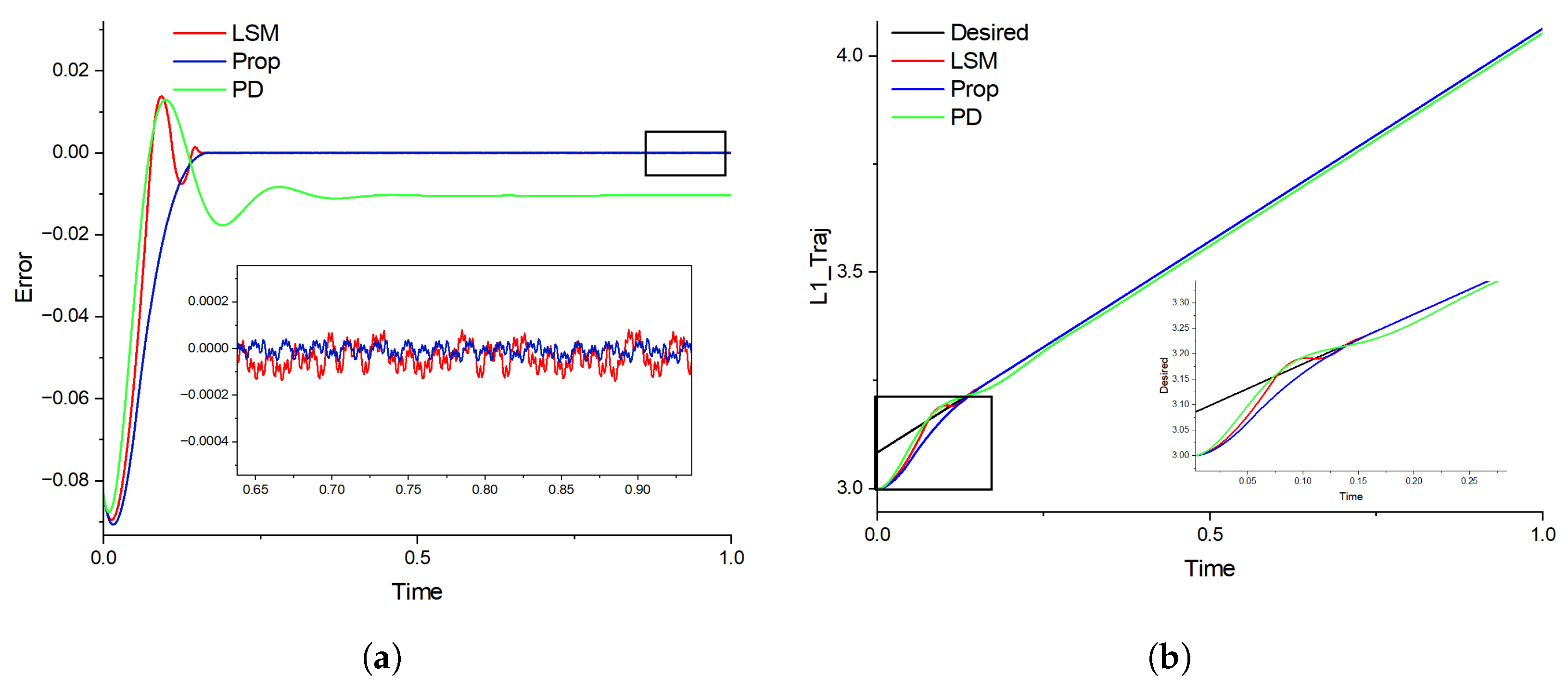
4.1. Case1: Vertical Lifting

The target motion is set to vertically lift the moving platform, where the desired lengths of the six legs are always equal. In this example, the controller parameters are set as $d_0=48,m=5,n=3,k=100,h_1=h_2=\cdots =h_6=0.4$. The parameters of the PD controller are $K_p=500$ and $K_d=10$. All simulation results were obtained under an external disturbance of ${[0;0;-10]}^T$. The linear SM controller is designed based on the sliding surface $s={\mathbf{e}}_{\mathbf{2}}+k_1{\mathbf{e}}_{\mathbf{1}}$, where ${\mathbf{e}}_{\mathbf{1}}$ represents the position error, and ${\mathbf{e}}_{\mathbf{2}}$ represents the velocity error. The control law applies a proportional control term to the velocity error and a discontinuous term to enforce the sliding condition. The control force of LSM is given by $f=-k_2{\mathbf{e}}_{\mathbf{2}}-k_1\mathrm{sign}\left(s\right)$. The key parameters are selected as follows: the sliding surface parameter $k_1=300$, the proportional control gain $k_2=8$, and the switching control gain $k_3=30$.

The tracking errors and performance for the vertical lifting task, using PD control, linear sliding mode control (LSM), and the proposed controller, are compared in Figure 5. Compared to PD control, the proposed method demonstrates faster convergence and reduced tracking errors. While LSM control exhibits oscillations over an extended period before the tracking error converges to zero, the proposed controller achieves convergence without overshoot or oscillations, and the steady-state error is approximately the same as that of the LSM.

A comparison of velocity tracking performance under various control laws, along with the associated leg output forces, is illustrated in Figure 6. PD control achieves a smoother and more stable tracking response, free from any chattering, albeit with a significantly slower convergence to the desired velocity trajectory. Conversely, both LSM and the proposed method exhibit faster tracking dynamics but at the expense of pronounced chattering. Notably, the proposed method demonstrates a substantial reduction in the amplitude of chattering compared to LSM, offering a superior trade-off between rapid tracking and minimizing high-frequency oscillations.

To mitigate the issue of chattering, the sign function in the controller can be replaced with a saturation function (Sat). The saturation function is defined as

$$\mathrm{sat}(x,\delta )=\left\{\begin{array}{cc}-1\hfill & x<-\delta \hfill \\ {\displaystyle \frac{x}{\delta }}\hfill & -\delta \le x\le \delta \hfill \\ 1\hfill & x>\delta \hfill \end{array}\right.$$

In this simulation experiment, the parameter $\delta$ of the saturation function is set to $1\times {10}^{-6}$. Figure 7 presents a comparison of the trajectory tracking error and control forces before and after replacing the sign function with the saturation function. It can be observed that, while the trajectory tracking error remains consistently small, the chattering in the control force is significantly reduced after the system stabilizes, resulting in smoother control behavior.

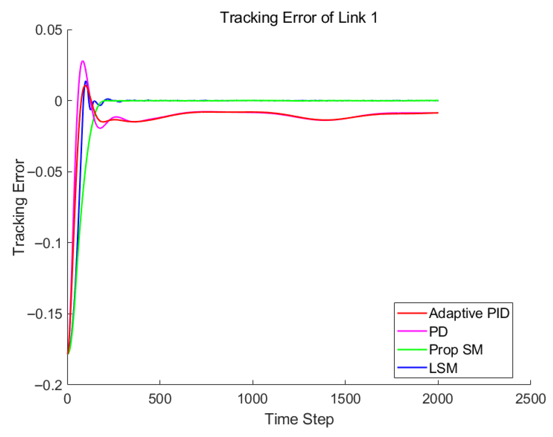
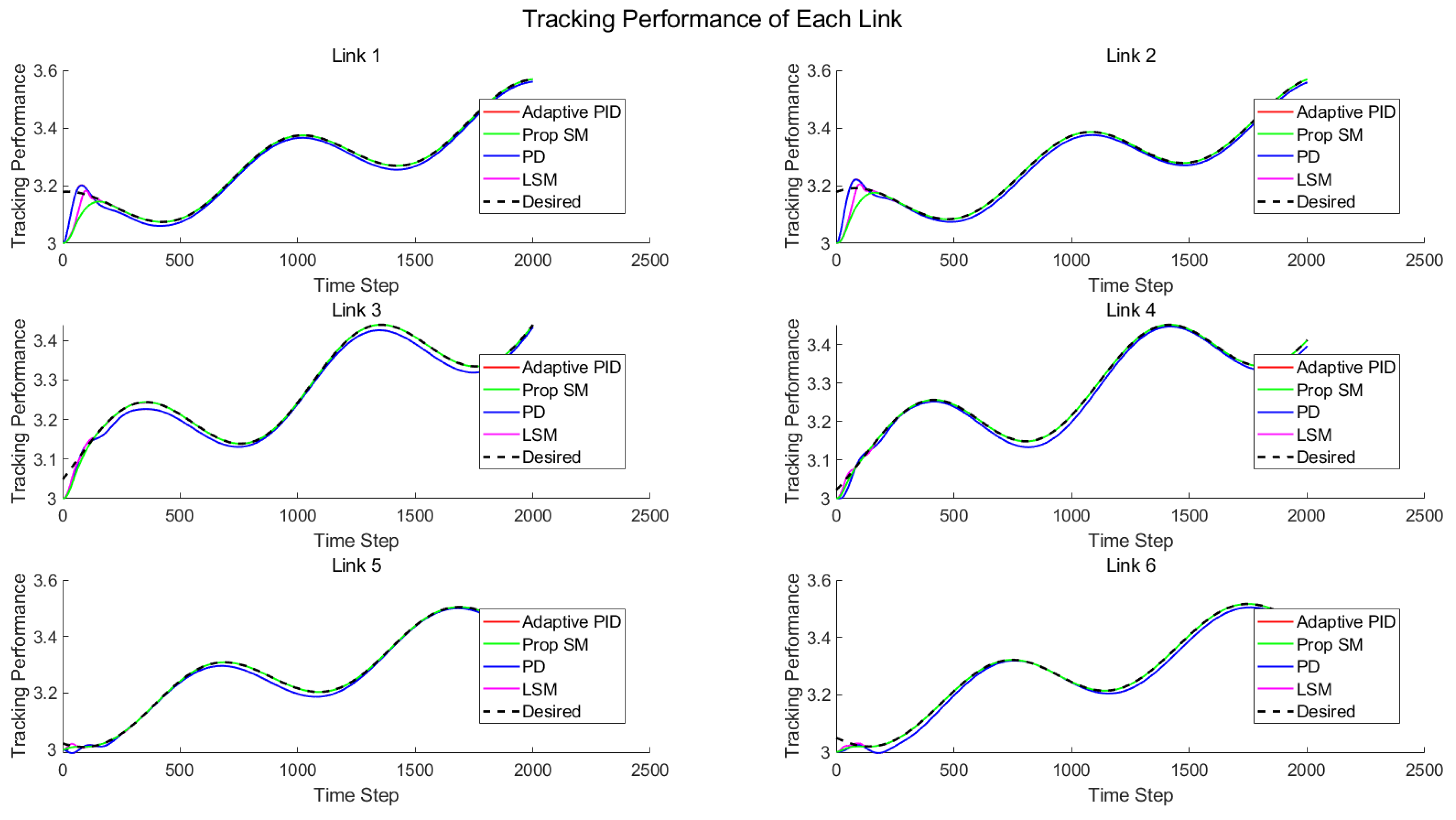
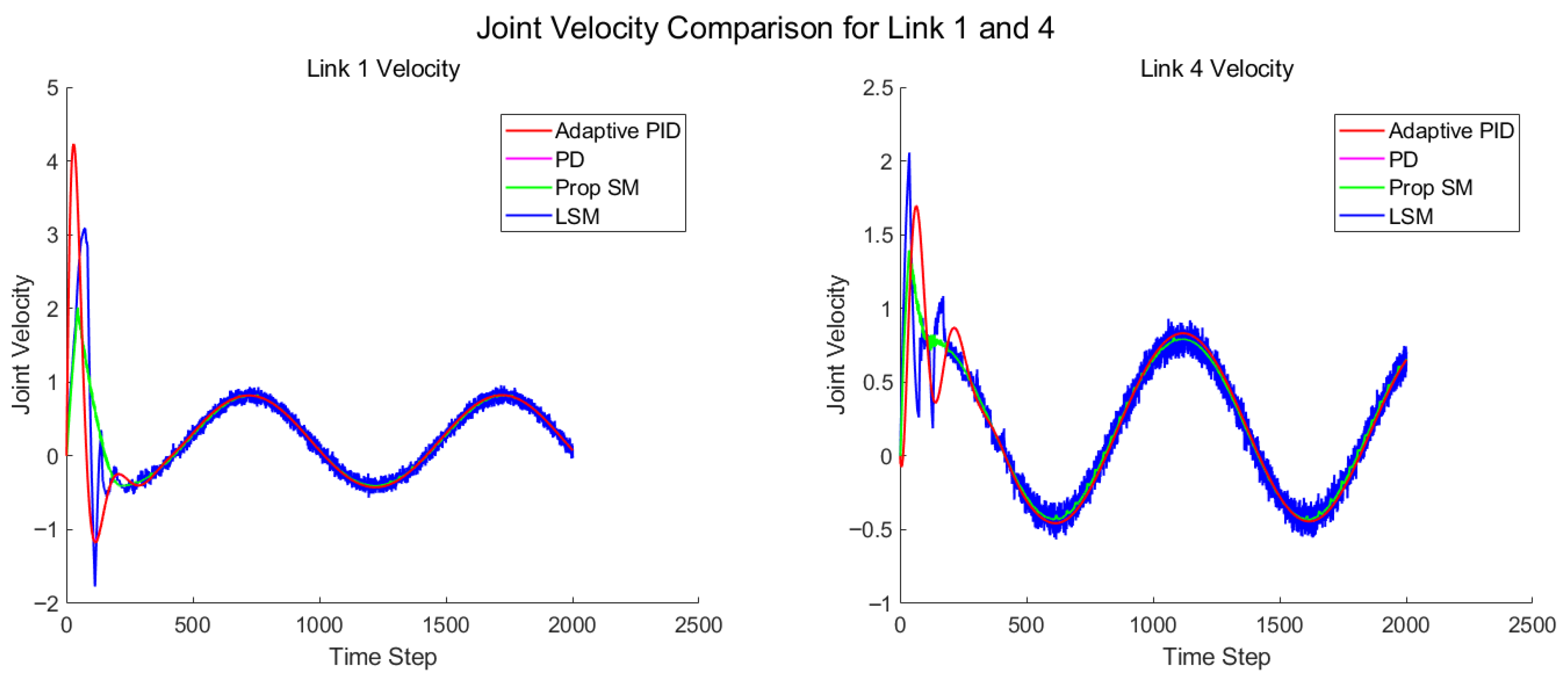
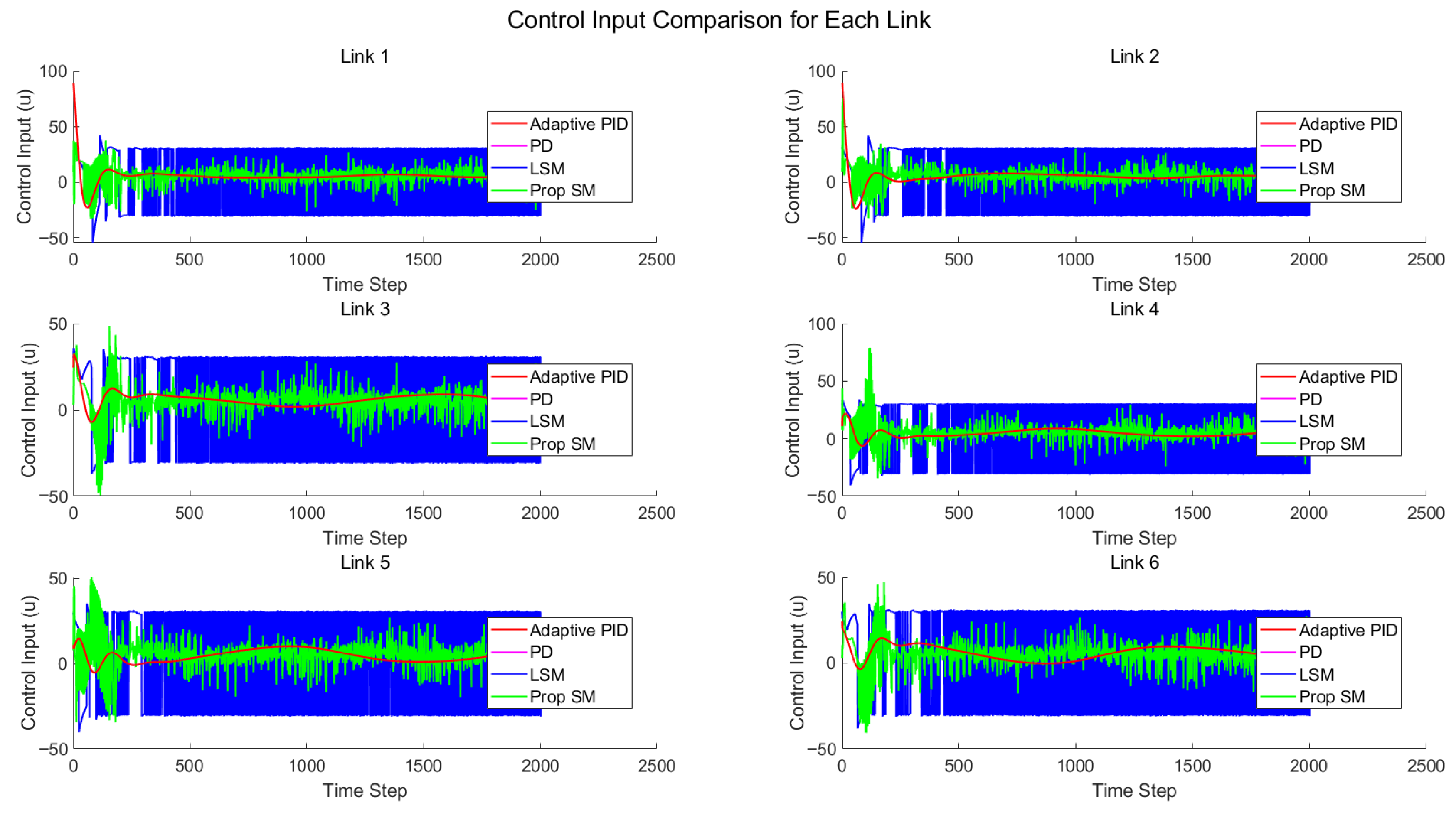
4.2. Case2: Complex Trajectory Tracking

To further evaluate the tracking performance of the controllers, a more complex trajectory involving simultaneous translational and rotational motion of the moving platform was used. The simulation parameters remained consistent with those of the vertical lifting scenario. As shown in Figure 8, the tracking errors of all six legs under PD, LSM, Adaptive PID, and the proposed method are compared. It can be observed that both LSM and the proposed method achieve significantly smaller tracking errors than the conventional PD controller. The Adaptive PID controller shows slightly improved performance over PD, particularly during periods of rapid trajectory variation, but still falls short of the precision achieved by the sliding-mode-based methods.

To provide a fair comparison, an Adaptive PID (APID) controller was introduced as a benchmark. This controller retains the conventional PID structure but updates its gain parameters online using adaptive laws. The initial values of the proportional, integral, and derivative gains were set to 500, 1, and 20, respectively, for each of the six legs. The learning rates for the adaptive update process were set as ${\gamma }_p=1000$, ${\gamma }_i=1000$, and ${\gamma }_d=500$, applied uniformly across all joints. These settings allow the controller to adjust its parameters in response to changing tracking errors while maintaining a balance between responsiveness and stability.

The tracking responses of the leg lengths under different control strategies—PD, LSM, Adaptive PID, the proposed method, and its saturation-augmented variant—are shown in Figure 9. In regions where the trajectory changes rapidly, the proposed method maintains low tracking errors and superior robustness. In contrast, the Adaptive PID controller exhibits noticeable deviations in such regions, while the LSM method demonstrates improved, yet still less stable, performance compared to the proposed approach.

Table 2. Average tracking error and convergence time of each method.

Method	Link 1	Link 2	Link 3	Link 4	Link 5	Link 6
Average Tracking Error
APID	0.0105	0.0100	0.0112	0.0099	0.0096	0.0114
PD	0.0105	0.0098	0.0122	0.0092	0.0086	0.0125
Prop SM	9.89 × 10−4	9.33 × 10−4	1.06 × 10−3	8.84 × 10−4	1.07 × 10−3	7.87 × 10−4
LSM	7.70 × 10−4	8.03 × 10−4	7.17 × 10−4	7.69 × 10−4	7.41 × 10−4	7.26 × 10−4
Convergence Time (time step = 1 ms)
APID	63	64	61	66	59	54
PD	101	107	53	63	60	44
Prop SM	198	191	186	139	166	325
LSM	490	264	608	485	566	513

summarizes the average tracking errors and convergence times of four control strategies. The average tracking error is calculated from the final 1 s of the simulation data, using the mean of the last 1000 time steps. The convergence time is defined as the earliest time step at which the tracking error remains continuously below twice the corresponding average error for at least 100 consecutive steps. It can be observed that the Prop SM and LSM controllers achieve significantly lower tracking errors, approximately one order of magnitude smaller than those of the APID and PD controllers. However, they also exhibit slower convergence times. In contrast, the APID and PD methods converge more quickly but maintain higher steady-state errors. This highlights a trade-off between convergence speed and steady-state accuracy across different control strategies.

As illustrated in Figure 10, the velocity tracking performance of links L1 and L4 under different control strategies is compared. The PD controller exhibits relatively large tracking errors, while both the LSM and the proposed method experience chattering due to the use of discontinuous control terms. However, the proposed method shows smaller chattering amplitude compared to LSM. The Adaptive PID controller demonstrates improved tracking accuracy over PD and produces smooth control signals without chattering, but its tracking precision is still lower than that of the sliding-mode-based methods.

Figure 11 illustrates the control forces generated by different control schemes under a complex motion trajectory, where PropSat refers to the proposed method with a saturation function. The results demonstrate that both the PD and Adaptive PID controllers produce relatively smooth control forces but suffer from larger tracking errors and slower convergence rates compared to the sliding-mode-based methods. In contrast, the LSM and the proposed method exhibit chattering due to the discontinuous nature of the control law. However, by replacing the sign function with a saturation function, the amplitude of chattering is significantly reduced, resulting in smoother control responses without sacrificing tracking performance.

Table 3. Control effort energy of each method (joules).

Method	Leg 1	Leg 2	Leg 3	Leg 4	Leg 5	Leg 6
APID	157.83	164.24	105.09	70.81	68.54	104.82
PD	157.05	163.37	104.25	70.62	68.10	103.77
Prop SM	180.68	182.88	186.74	195.37	195.14	185.32
LSM	1.81 × 103	1.81 × 103	1.83 × 103	1.84 × 103	1.85 × 103	1.83 × 103

presents the control effort of each method across all six legs. The proposed method (Prop SM) requires moderate effort, averaging around 187 N²·s per leg. This is higher than that of APID and PD controllers (about 112 N²·s) but significantly lower than the LSM controller, which exceeds 1800 N²·s per leg. This indicates that the proposed method achieves a substantial reduction in tracking error at the cost of slightly increased control effort while remaining far more energy-efficient than conventional sliding mode control.

4.3. Case3: Tracking with Disturbances

An external disturbance is applied at $t=1\mathrm{s}$ to evaluate controller robustness. The applied force and torque switch from

$$f_{\mathrm{ext}}=\left[\begin{array}{c}0\\ 0\\ -10\end{array}\right],n_{\mathrm{ext}}=\left[\begin{array}{c}0\\ 0\\ 0\end{array}\right]$$

to

$$f_{\mathrm{ext}}=\left[\begin{array}{c}0\\ 0\\ -100\end{array}\right],n_{\mathrm{ext}}=\left[\begin{array}{c}0\\ 0\\ 10\end{array}\right].$$

Figure 12 shows the tracking error of the platform under disturbance. Figure 13 presents the actual tracking trajectories. After $t=1\mathrm{s}$, both PD and APID controllers experience a significant increase in error, while the proposed sliding mode (Prop SM) controller maintains a consistently low level of error throughout.

Figure 14 illustrates the control force outputs. It can be observed that the Prop SM controller responds rapidly with a sharp change in force at the moment of disturbance, indicating strong disturbance rejection. In contrast, the forces generated by APID and PD do not adjust quickly enough, leading to poor compensation.

4.4. Case4: Efficient Forward Kinematics

In order to investigate efficient solution methods for forward kinematics, we trained a neural network model (NET) and SVR using the same dataset. The neural network consists of two hidden layers, with 15 and 10 nodes, respectively. The activation function used in both hidden layers is tansig, and the output layer uses the purelin activation function.

To compare the advantages of SVR over NET in solving the forward kinematics problem of the GSP, we randomly selected 2000 reachable points. For each point, the initial value for the iterative solution was computed using both SVR and Net. Subsequently, the Levenberg–Marquardt method was employed to iteratively solve for a solution that meets the accuracy requirements. The total computation time for each method is presented in Figure 15.

From the results, it can be concluded that the mean computation time required for generating the initial value using SVR is consistently lower than that of Net. This discrepancy is likely due to the lower computational complexity of SVR compared to Net. Even for a relatively simple neural network structure, its computational overhead is still higher than that of SVR. On the other hand, the time required for the iterative solving process remains similar for both methods. These findings highlight the superiority of SVR in solving the kinematics problem of parallel mechanisms, particularly in terms of computational efficiency.

5. Conclusions

This study proposed an efficient forward kinematics solution algorithm that combines Support Vector Regression (SVR) with the Levenberg–Marquardt method, applied to trajectory tracking control of a six-degree-of-freedom Gough–Stewart platform (GSP). By designing a sliding mode (SM) controller, high-precision trajectory tracking was achieved under complex dynamic conditions. The experimental results show that the proposed method not only improves the speed and accuracy of forward kinematics computation but also significantly enhances the robustness and disturbance rejection capabilities of the controller, especially in the presence of model deviations and external disturbances. In particular, under sudden force and torque disturbances, the SM controller maintained a low tracking error and responded rapidly with effective control force adjustment, while PD and adaptive PID controllers exhibited degraded performance. This work provides a novel approach to addressing the control challenges of GSPs, with promising application prospects. However, it is important to note that, due to constraints in our laboratory conditions, physical experiments were not conducted to validate the proposed method. We sincerely regret this limitation and hope that future studies will provide experimental validation to further substantiate the findings presented herein.

In future work, we aim to focus on several key areas: optimizing the control algorithm to enhance computational efficiency and convergence rates while addressing real-time performance challenges in practical applications. Additionally, efforts will be made to improve the system’s robustness under varying environmental conditions and external disturbances and to expand the system’s scalability for larger platforms. Furthermore, we plan to explore the integration of machine learning techniques for adaptive control. If conditions permit, we are also keen to perform physical experiments to validate the proposed algorithm under real-world conditions, which will provide further insights into its performance and robustness. We believe that such experimental verification will contribute significantly to improving the algorithm’s practical applicability and performance.

References

1. Duong, T.T.C.; Nguyen, C.C.; Tran, T.D. Experimental Investigation of Motion Control of a Closed-Kinematic Chain Robot Manipulator Using Synchronization Sliding Mode Method with Time Delay Estimation. Appl. Sci. 2025, 15, 5206. [Google Scholar] [CrossRef]
2. Vu, M.T.; Alattas, K.A.; Bouteraa, Y.; Rahmani, R.; Fekih, A.; Mobayen, S.; Assawinchaichote, W. Optimized Fuzzy Enhanced Robust Control Design for a Stewart Parallel Robot. Mathematics 2022, 10, 1917. [Google Scholar] [CrossRef]
3. Xie, B.; Dai, S. Robust Terminal Sliding Mode Control on SE(3) for Gough–Stewart Flight Simulator Motion Platform with Payload Uncertainty. Electronics 2022, 11, 814. [Google Scholar] [CrossRef]
4. Nguyen, T.T.; Nguyen, C.C.; Nguyen, T.M.; Duong, T.T.C.; Ngo, H.T.T.; Sun, L. Decentralized Adaptive Control of Closed-Kinematic Chain Mechanism Manipulators. Machines 2025, 13, 331. [Google Scholar] [CrossRef]
5. Jing, X.; Li, C. Dynamic Modeling and Solution of 6-DOF Parallel Mechanism. IEEE Access 2022, 10, 33695–33703. [Google Scholar] [CrossRef]
6. Chen, X.; Zhao, F.; Liu, Y.; Liu, H.; Huang, T.; Qiu, J. Reduced-Order Observer-Based Preassigned Finite-Time Control of Nonlinear Systems and Its Applications. IEEE Trans. Syst. Man Cybern. Syst. 2023, 53, 4205–4215. [Google Scholar] [CrossRef]
7. Huang, X.; Liao, Q.; Wei, S.; Qiang, X.; Huang, S. Forward Kinematics of the 6-6 Stewart Platform with Planar Base and Platform Using Algebraic Elimination. In Proceedings of the 2007 IEEE International Conference on Automation and Logistics, Jinan, China, 18–21 August 2007; pp. 2655–2659. [Google Scholar] [CrossRef]
8. Sheng, L.; Wan-long, L.; Yan-chun, D.; Liang, F. Forward kinematics of the Stewart platform using hybrid immune genetic algorithm. In Proceedings of the 2006 International Conference on Mechatronics and Automation, Luoyang, China, 25–28 June 2006; pp. 2330–2335. [Google Scholar] [CrossRef]
9. Tarokh, M. Real Time Forward Kinematics Solutions for General Stewart Platforms. In Proceedings of the 2007 IEEE International Conference on Robotics and Automation, Rome, Italy, 10–14 April 2007; pp. 901–906. [Google Scholar] [CrossRef]
10. Yang, X.; Wu, H.; Chen, B.; Li, Y.; Jiang, S. A dual quaternion approach to efficient determination of the maximal singularity-free joint space and workspace of six-DOF parallel robots. Mech. Mach. Theory 2018, 129, 279–292. [Google Scholar] [CrossRef]
11. Chen, S.H.; Fu, L.C. The Forward Kinematics of the 6-6 Stewart Platform Using Extra Sensors. In Proceedings of the 2006 IEEE International Conference on Systems, Man and Cybernetics, Taipei, Taiwan, 8–11 October 2006; Volume 6, pp. 4671–4676. [Google Scholar] [CrossRef]
12. Sang, L.H.; Han, M.C. The estimation for forward kinematic solution of Stewart platform using the neural network. In Proceedings of the 1999 IEEE/RSJ International Conference on Intelligent Robots and Systems. Human and Environment Friendly Robots with High Intelligence and Emotional Quotients (Cat. No.99CH36289), Kyongju, Republic of Korea, 17–21 October 1999; Volume 1, pp. 501–506. [Google Scholar] [CrossRef]
13. Chauhan, D.K.S.; Vundavilli, P.R. Forward kinematics of the Stewart parallel manipulator using machine learning. Int. J. Comput. Methods 2022, 19, 2142009. [Google Scholar] [CrossRef]
14. Huang, T.; Wang, J.; Pan, H. Adaptive bioinspired preview suspension control with constrained velocity planning for autonomous vehicles. IEEE Trans. Intell. Veh. 2023, 8, 3925–3935. [Google Scholar] [CrossRef]
15. Sosa-Méndez, D.; Lugo-González, E.; Arias-Montiel, M.; Garcia-Garcia, R.A. ADAMS-MATLAB co-simulation for kinematics, dynamics, and control of the Stewart–Gough platform. Int. J. Adv. Robot. Syst. 2017, 14, 1729881417719824. [Google Scholar] [CrossRef]
16. Huang, C.I.; Wang, R.S. Hybrid control based on type-2 fuzzy-iterative learning control strategies with stewart platform for repetitive trajectories. In Proceedings of the 2015 10th Asian Control Conference (ASCC), Kota Kinabalu, Malaysia, 31 May–3 June 2015; IEEE: Piscataway, NJ, USA, 2015; pp. 1–5. [Google Scholar]
17. Zhou, Y.; She, J.; Wang, F.; Iwasaki, M. Disturbance Rejection for Stewart Platform Based on Integration of Equivalent-Input- Disturbance and Sliding-Mode Control Methods. IEEE/ASME Trans. Mechatronics 2023, 28, 2364–2374. [Google Scholar] [CrossRef]
18. Dai, X.; Song, S.; Xu, W.; Huang, Z.; Gong, D. Modal space neural network compensation control for Gough-Stewart robot with uncertain load. Neurocomputing 2021, 449, 245–257. [Google Scholar] [CrossRef]
19. Lafmejani, A.S.; Masouleh, M.T.; Kalhor, A. Trajectory tracking control of a pneumatically actuated 6-DOF Gough–Stewart parallel robot using Backstepping-Sliding Mode controller and geometry-based quasi forward kinematic method. Robot. Comput.-Integr. Manuf. 2018, 54, 96–114. [Google Scholar] [CrossRef]
20. Kalani, H.; Rezaei, A.; Akbarzadeh, A. Improved general solution for the dynamic modeling of Gough–Stewart platform based on principle of virtual work. Nonlinear Dyn. 2016, 83, 2393–2418. [Google Scholar] [CrossRef]
21. Gallardo, J.; Rico, J.; Frisoli, A.; Checcacci, D.; Bergamasco, M. Dynamics of parallel manipulators by means of screw theory. Mech. Mach. Theory 2003, 38, 1113–1131. [Google Scholar] [CrossRef]
22. Liu, M.J.; Li, C.X.; Li, C.N. Dynamics analysis of the Gough-Stewart platform manipulator. IEEE Trans. Robot. Autom. 2000, 16, 94–98. [Google Scholar] [CrossRef]
23. Khalil, W.; Guegan, S. Inverse and direct dynamic modeling of Gough-Stewart robots. IEEE Trans. Robot. 2004, 20, 754–761. [Google Scholar] [CrossRef]
24. Liu, Y.; Liu, X.; Jing, Y.; Chen, X.; Qiu, J. Direct adaptive preassigned finite-time control with time-delay and quantized input using neural network. IEEE Trans. Neural Netw. Learn. Syst. 2019, 31, 1222–1231. [Google Scholar] [CrossRef]
25. Chen, X.; Hu, S.; Xie, X.; Qiu, J. Consensus-Based Distributed Secondary Control of Microgrids: A Pre-Assigned Time Sliding Mode Approach. IEEE/CAA J. Autom. Sin. 2024, 11, 2525–2527. [Google Scholar] [CrossRef]
26. Chen, X.; Huang, T.; Cao, J.; Park, J.H.; Qiu, J. Finite-time multi-switching sliding mode synchronisation for multiple uncertain complex chaotic systems with network transmission mode. IET Control. Theory Appl. 2019, 13, 1246–1257. [Google Scholar] [CrossRef]
27. Gu, Y.; Shen, M.; Park, J.H.; Wang, Q.G.; Zhu, Z.H. Dynamic Guaranteed Cost Event-Triggered-Based Anti-Disturbance Control of T-S Fuzzy Wind-Turbine Systems Subject to External Disturbances. IEEE Trans. Fuzzy Syst. 2024, 32, 7063–7072. [Google Scholar] [CrossRef]
28. Tian, Y.; Shi, Y.; Shao, X.; Hu, Q.; Yang, H.; Zhu, Z.H. Spacecraft Proximity Operations Under Motion and Input Constraints: A Learning-Based Robust Optimal Control Approach. IEEE Trans. Aerosp. Electron. Syst. 2024, 60, 7838–7852. [Google Scholar] [CrossRef]
29. Zhou, W.; Cheng, H.; Chen, Z.; Hua, M. Adaptive Sliding Mode Fault-Tolerant Tracking Control for Underactuated Unmanned Surface Vehicles. J. Mar. Sci. Eng. 2025, 13, 712. [Google Scholar] [CrossRef]
30. Ahn, H.; Kim, S.; Park, J.; Chung, Y.; Hu, M.; You, K. Adaptive Quick Sliding Mode Reaching Law and Disturbance Observer for Robust PMSM Control Systems. Actuators 2024, 13, 136. [Google Scholar] [CrossRef]
31. Huang, T.; Pan, H.; Sun, W.; Gao, H. Sine resistance network-based motion planning approach for autonomous electric vehicles in dynamic environments. IEEE Trans. Transp. Electrif. 2022, 8, 2862–2873. [Google Scholar] [CrossRef]
32. Keshavan, J.; Belgaonkar, S.; Murali, S. Adaptive Control of a Constrained First Order Sliding Mode for Visual Formation Convergence Applications. IEEE Access 2023, 11, 112263–112275. [Google Scholar] [CrossRef]
33. Huang, T.; Wang, J.; Pan, H.; Sun, W. Finite-time fault-tolerant integrated motion control for autonomous vehicles with prescribed performance. IEEE Trans. Transp. Electrif. 2022, 9, 4255–4265. [Google Scholar] [CrossRef]
34. Kamal, S.; Chalanga, A.; Bandyopadhyay, B. Multivariable continuous integral sliding mode control. In Proceedings of the 2015 International Workshop on Recent Advances in Sliding Modes (RASM), Istanbul, Turkey, 9–11 April 2015; IEEE: Piscatway, NJ, USA, 2015; pp. 1–5. [Google Scholar]
35. Amirkhani, S.; Mobayen, S.; Iliaee, N.; Boubaker, O.; Hosseinnia, S.H. Fast terminal sliding mode tracking control of nonlinear uncertain mass–spring system with experimental verifications. Int. J. Adv. Robot. Syst. 2019, 16, 1729881419828176. [Google Scholar] [CrossRef]
36. Huang, T.; Wang, J.; Pan, H. Approximation-Free Prespecified Time Bionic Reliable Control for Vehicle Suspension. IEEE Trans. Autom. Sci. Eng. 2024, 21, 5333–5343. [Google Scholar] [CrossRef]
37. Zhai, J.; Xu, G. A novel non-singular terminal sliding mode trajectory tracking control for robotic manipulators. IEEE Trans. Circuits Syst. II Express Briefs 2020, 68, 391–395. [Google Scholar] [CrossRef]
Figure 1. (a) The structure of the GSP. (b) The closed-loop vectors of the Stewart platform.
Electronics 14 02872 g001
Figure 2. Illustration of SVR.
Electronics 14 02872 g002
Figure 3. Overall framework.
Electronics 14 02872 g003
Figure 4. Kinematics process.
Electronics 14 02872 g004
Figure 5. (a) Comparison of tracking errors. (b) Comparison of tracking performance.
Electronics 14 02872 g005
Figure 6. (a) Comparison of velocity errors. (b) Comparison of control forces.
Electronics 14 02872 g006
Figure 7. (a) Error comparison of sat and sign function. (b) Control force of sat and sign function.
Electronics 14 02872 g007
Figure 8. Tracking error of the link 1.
Electronics 14 02872 g008
Figure 9. Tracking performance of the six legs.
Electronics 14 02872 g009
Figure 10. Velocity tracking performance of L1 and L4.
Electronics 14 02872 g010
Figure 11. Force of 6 Legs.
Electronics 14 02872 g011
Figure 12. Tracking error of the Stewart platform under external disturbances.
Electronics 14 02872 g012
Figure 13. Tracking trajectories of the Stewart platform under disturbances.
Electronics 14 02872 g013
Figure 14. Control force response of each controller under disturbances.
Electronics 14 02872 g014
Figure 15. Solving time using NET and SVR.
Electronics 14 02872 g015