
Fault Diagnosis Method of Planetary Gearbox Based on Compressed Sensing and Transfer Learning

1
Shijiazhuang Campus, Army Engineering University of PLA, Shijiazhuang 050003, China
2
Hebei Key Laboratory of Condition Monitoring and Assessment of Mechanical Equipment, Shijiazhuang 050003, China
*
Author to whom correspondence should be addressed.
Electronics 2022, 11(11), 1708; https://doi.org/10.3390/electronics11111708
Submission received: 19 April 2022
/
Revised: 22 May 2022
/
Accepted: 24 May 2022
/
Published: 27 May 2022
(This article belongs to the Special Issue Deep Learning Algorithm Generalization for Complex Industrial Systems)
Abstract
:This paper suggests a novel method for diagnosing planetary gearbox faults. It addresses the issue of network bandwidth limitation during wireless data transmission and the problem of relying on expert experience and insufficient training samples in traditional fault diagnosis. The continuous wavelet transform was combined with the AlexNet convolutional neural network using transfer learning and the compressed theory of sense. The original vibration signal was compressed and reconstructed using the compressed sampling orthogonal matching pursuit reconstruction algorithm. A continuous wavelet transform was used to convert the compressed signal into a time–frequency image. The pretrained AlexNet model was selected as the migration object, the network model was fine-tuned and retrained, and the trained AlexNet model was used to diagnose the fault using the model-based migration method. It was demonstrated by the experimental results when the compression ratio CR = 0.5. Compared to other network models, the classification accuracy rate is 97.78%. This method has specific reference value and application prospects and good feature extraction and fault classification capabilities.
1. Introduction
Online monitoring of rotating machinery equipment status has become critical in intelligent manufacturing. The mechanical structure has become more complicated and extensive as science and technology progress, and the operating environment is harsh. When rotating machinery fails, it causes a production shutdown or a safety accident [1]. As a result, it is critical to extract valuable information from massive historical data. As a result, the health status assessment of the current working condition of the equipment can be carried out effectively.
Nonetheless, real-time monitoring and fault diagnosis are underway, posing significant challenges to data transmission, network bandwidth, and data storage. The generation of a large amount of redundant data will result in the waste of resources. Data compression and intelligent fault diagnosis have evolved into research hotspots, offering practical solutions to the abovementioned problems [2,3]. Data compression technology, for example, has been widely used in image and video processing, with numerous research results [4,5].
In recent years, conventional fault diagnosis has been divided into data collection, vibration signal characteristic parameter extraction, and fault classification. It includes a variety of fault diagnosis implementation methods. The equipment vibration signal collection is realized using the Nyquist sampling theorem [6]. There are primarily two techniques for extracting feature parameters in the time and frequency domains [7,8]. Statistical and model methods are used in time-domain plans [9], while envelope analysis and cepstral analysis are used in frequency domain plans [10,11]. Following the extraction of feature parameters, the following fault diagnosis models are used: K-nearest neighbor classification [12], random forest [13], and support vector machine [14]. Although traditional fault diagnosis technology has produced notable results when rotating machinery is considered [15,16], the following limitations remain:
- When the vibration signal acquisition process is run, many redundant observations are generated, which is incompatible with wireless transmission and data storage. As a result, advanced sensing technology must be used to compress and rebuild the original signal;
- The vibration signal is nonstationary, and the extracted characteristic parameters include random noise. As a result, it is sufficient to use noise reduction technology to preprocess the signal before extracting the characteristic parameters from the weak signal;
- The extracted time domain and frequency domain feature parameters rely on expert, prior knowledge. When the feature parameters are incorrectly set, the precision of the fault diagnosis outcomes suffers;
This article focuses primarily on vibration signal compression and reconstruction, feature parameter extraction, and the development of a deep network structure model.
Compressed sensing technology has solved the problems of wireless data transmission and storage in recent years. Still, it has also played an essential role in the fault diagnosis of rotating machinery. Compressed sensing technology can significantly reduce the processing time of massive data and improve fault diagnosis efficiency, allowing for real-time online fault diagnosis of equipment. As a result, the equipment’s safety and stability are effectively improved, and the risks and economic losses caused by equipment failures are avoided. It is now gradually becoming a research hotspot in this field.
Xing et al. [19] proposed using multimodal recombination methods to compress and reconstruct data. To diagnose fault detection, they advocate for the use of the least-squares planning algorithm. Shi et al. [20] proposed a sparse autoencoder and compressed sensing technique. The wavelet packet’s energy entropy reduces feature dimensionality, and the general sparse autoencoder is used for classification. Shao et al. [21] proposed a diagnosis method that combines an advanced convolutional deep belief network with the sense of compression. The moving average process of finger data improves the model’s generalization capability. Shi et al. [22] directly extracted characteristic fault parameters from compressed data using compressed sensing technology.
Deep learning (DL) has gradually grown into an efficient method to solve the problems’ conventional fault-diagnosing approaches face as artificial intelligence develops rapidly. It also has the powerful ability to automatically extract valuable feature parameters, allowing it to avoid reliance on noise reduction technology and expert knowledge effectively. Deep learning techniques that are commonly used include Convolutional Neural Network (CNN) [23], Deep Belief Network (DBN) [24], and Long Short-term Memory Network (LSTM) [25]. They first used CNN in research to process images and recognize speeches. Many researchers have applied CNN technology to fault diagnosis [26,27,28], which has proven to be a popular research topic. He et al. [29] proposed a 1D-CNN deep transfer learning approach, Adopt Adam optimizer, to improve fault diagnosis precision. Xu and colleagues [30] propose a fault diagnosis method that combines CNN and the deep forest (gcForest) model, significantly improving fault diagnosis accuracy. Xin et al. [31] proposed a multiobjective deep convolutional neural network diagnosis method that uses data about time, frequency, and time–frequency as input conditions to detect faults. Zhao et al. [32] proposed a convolutional neural network (CNN) diagnosis method that combines batch normalization and finger data moving average. When different settings are assumed, this method has an excellent diagnostic effect. However, deep learning has achieved remarkable results in fault diagnosis in the studies mentioned above. However, processing large amounts of data in practical engineering applications and consuming computing resources are still required. Because of the harsh working environment, vibration signals containing many noise signals are produced, significantly increasing the difficulty of using one-dimensional signals for diagnosis.
Intelligent monitoring and equipment health assessments have entered the significant data phase, and higher demands have been proposed. Data compression is critical because it reduces storage requirements while also lowering network bandwidth requirements. This manuscript offers a method for diagnosing faults that combines sense compression and transfer learning. This method compresses and reconstructs the collected original vibration signal; the compressed signal is then transformed into an image represented by a time–frequency by continuous wavelet transform; and finally, an efficient deep transfer learning model is built. As the migration target, a pretrained AlexNet network model is selected. In addition, the new fully connected layer parameters are randomly initialized and retrained. The experiment results indicated that the model could extract robust features and classify faults.
This paper’s main contributions are as follows:
- Using the Compressive Sampling Orthogonal Matching Pursuit algorithm, the optimal global solution is gradually approximated by finding the optimal local solution in each iteration. The most relevant one is seen from the absolute value of the inner product: the residuals. Compared with other traditional compression algorithm methods, this method can effectively improve data network transmission’s work efficiency and show a better compression effect and reconstruction accuracy.
- A fault diagnosis method is proposed based on the combination of compressed sensing technology and transfer learning. Compared with other deep understanding and traditional machine learning methods, under a high compression rate, this method has the advantages of a simple network model structure, strong fault–feature extraction ability, high classification accuracy, small calculation amount, and short running time. In addition, the method has good portability and can be applied to embedded systems based on edge computing.
The remainder of this manuscript is arranged as the following: Part 2 introduces the basic theory of continuous wavelet transform and compressive sampling orthogonal matching pursuit algorithm. Part 3 presents the structure principle of deep convolutional neural networks and the description and analysis of transfer learning. Part 4 describes the process of fault diagnosis based on compressed sensing and deep transfer learning. Part 5 verifies the proposed method through experiments and analyzes the experimental results, and the final part, Part 6, presents the conclusions.
2. Continue Wavelet Transform and Compressed Sensing
2.1. Continue Wavelet Transform
Continuous Wavelet Transform (CWT) is a generally employed time–frequency domain investigation approach. This method effectively maintains the localization advantage of STFT (Short-Time Fourier Transform, STFT) and solves the defect that the window size does not change with frequency. A “Time-Frequency” window that varies with frequency can be achieved to some extent. At the same time, it exhibits the advantages of good local representation ability and multiresolution. It is extensively used when the vibration signal analysis of rotating machinery is under consideration [33]. The transformation Equation is defined by:
In the Equation, x(t) represents the original vibration signal; α represents the scale parameter; β represents the transformation parameter; and represents the coefficient of the wavelet. represents the basic function of the wavelet. After running continuous wavelet transformations, the one-dimensional vibration signal x(t) can be converted into the coefficient matrix of two dimensions , and the corresponding time–frequency diagram can be obtained.
2.2. Compressed Sensing
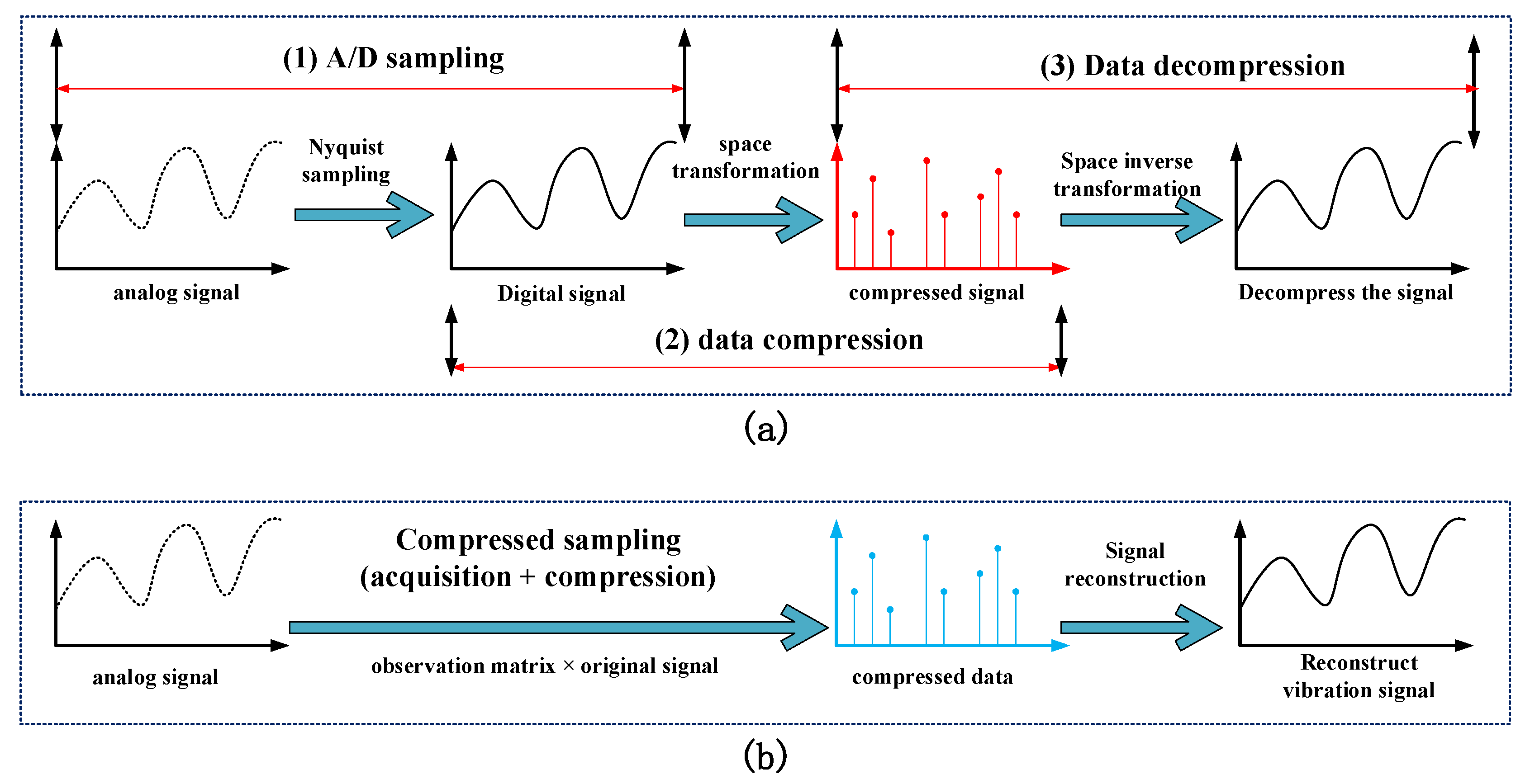
In 2006, Donoho et al. proposed the basic theory of Compressive Sensing (CS) at Stanford University in the United States [34]. CS technology breaks through the limitation of the traditional signal sampling theorem, integrates the signal acquisition and compression process, and contains the most valuable data in a small number of signals. In the conventional compression process, the Nyquist theorem is used to convert the analog signal into a digital signal, and wavelet transformation or discrete cosine transform is used to compress, store, and transmit the original signal. The sampled data is then decompressed using different fitting strategies and interpolations to recover the original vibration signal in a lossy or lossless manner. In compressed sensing, the analog signal is directly subjected to linear projection (i.e., observation matrix × original signal) to obtain a compressed signal. A reconstruction algorithm is used to restore the compressed signal at the receiving end. Figure 1 depicts a comparative analysis of the traditional compression process and the compressed sensing operation.
2.3. Compressed Sampling Orthogonal Matching Pursuit Reconstruction Algorithm
In 2008, D. Needell et al. proposed the basic theory of Compressive Sampling Orthogonal Matching Pursuit (CoSaMP) [35]. This algorithm is greedy. The CoSaMP algorithm finds the largest element in each iteration and picks the most suitable atom to gradually build a sparse approximation. No matter whether it is a common or sparse signal, the CoSaMP algorithm has high constraints on the computational cost and storage requirements, so the CoSaMP algorithm is effective in solving the problem. The specific process of the CoSaMP algorithm is as follows:
Input: observation vector y, M × N dimension measurement matrix A, Sparsity k.
Output: The original vibration signal X approximates X′.
Step 1: Initialization. Residual r0 = y, number of iterations t = 1, index set Λ0 = Ø.
Step 2: Calculate the correlation between the observation matrix A and the residual r, and find the index of the atom when the 2k maximum matches are:
In the formula, dj is the atom in the observation matrix A.
Step 3: Update the set of candidate atoms.
Step 4: Solve the set corresponding to the k atoms with the largest inner product of the candidate atom matrix At and the observation vector.
Step 5: Update Signal Approximation by Least Squares.
Step 6: Update residual values and number of iterations.
Step 7: If t > k, stop the iteration and output the reconstructed signal, otherwise continue to Step 2.
3. Deep Convolutional Neural Networks and Transfer Learning
3.1. Deep Convolutional Neural Network based on AlexNet
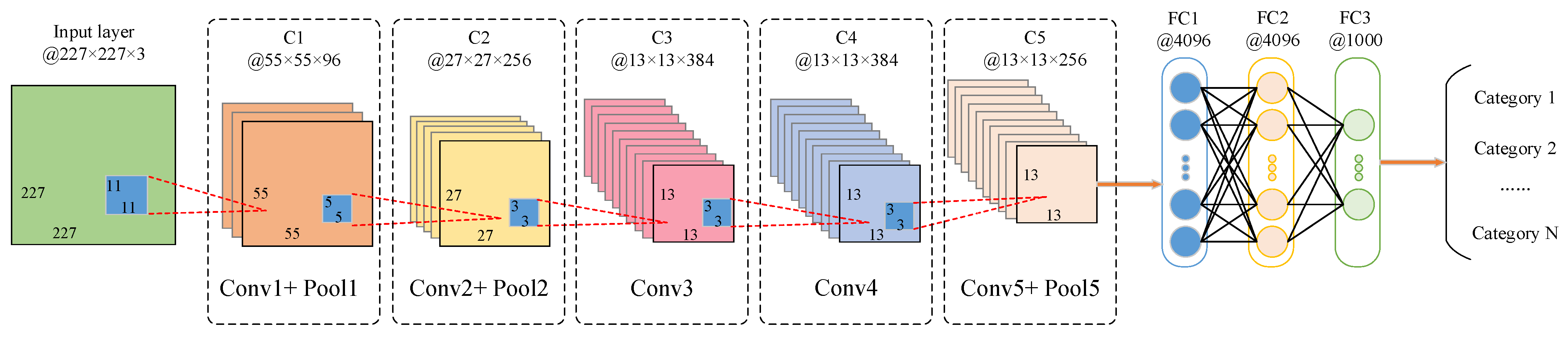
Compared with the traditional neural network [36], the AlexNet network model, with a deeper network structure, can better extract image features and learning capabilities. The AlexNet network model structure includes: five convolutional, three pooling, and three fully joined layers. Figure 2 presents them.
3.1.1. Convolutional Layer (CL)
The AlexNet network model has a convolutional layer (CL) called the core, and most of the feature extraction calculation functions are completed in the CL. By extracting different feature parameters in the image through multiple convolution kernels, the convolution outcomes are imported into the function, called activation, to form the feature mapping of the current layer. Computing convolution is denoted by
In the formula, L is the current layer number; denotes the i-th input feature mapping of the L-1 layer; denotes the j-th output feature mapping of the L-th convolutional layer; denotes the convolution kernel of the L-th convolution layer; Mj denotes the input feature mapping; f denotes the activation function.
After the convolutional layer, the ReLU activation function is generally used to replace the traditional Sigmod activation function. It helps enhance the training speed of the network and avoid the disappearance of the gradient, as shown in the following formula:
3.1.2. Pooling Layer (PL)
The pooling layer (PL) generally includes the mean PL and the highest PL. The pooling operation has the characteristics of scale invariance, which reduces the number of parameters while extracting the essential features. The overfitting can be avoided efficiently, thereby enhancing the model’s generalization capability. The maximum PL is used to attain the total value of each neural unit in the feature mapping to build the PL.
3.1.3. Softmax classifier
A wholly joined layer generally appears at the last stage of the network, connecting the weights of all neurons between layers. Using the softmax function, the two-dimensional features derived by the CL and PL will output a vector and map it between [0, 1] to achieve multiclassification tasks. After the softmax function regression processing, the output vector is converted into a probability distribution, and the corresponding expression is:
Among them: PL denotes the output of the completely joined layer; χL−1 denotes the input of the completely joined layer; ωL denotes the weight coefficient; bL denotes the bias of the L-th CL.
3.2. Transfer Learning (TL)
When the training and updating of the DL model are under consideration, a lot of calculation time and correct manual annotation are required. The labeling of massive data requires a lot of time and high cost, bringing new challenges to deep learning. However, the use of transfer learning methods can effectively solve such problems [37].
Transfer learning is a significant division of machine learning. TL can utilize the similarities between data, models, and tasks thoroughly, and transfer the knowledge and models learned in the source domain to the target domain. This paper adopts the model-based TL approach (MBTL) [38]. It relates to finding the feature parameters of the model that can be shared from both source and target domains to realize TL, as shown in Figure 3. Compared with other networks, the AlexNet network has the advantages of solid fault–feature extraction ability, simple network structure, fewer parameters, and fast convergence speed [39]. Therefore, to build an efficient deep transfer learning model, one must choose five convolutional layers of a pretrained AlexNet network model as the migration target, randomly initialize the new fully connected layer parameters, and migrate the basic image features of the ImageNet dataset (containing more than 1.2 million images and 1000 categories) to the planetary gearbox dataset. Although the classification in the ImageNet data set is very different from the vibration signal of the planetary gearbox, the essential characteristics remain the same. The continuous wavelet transform is employed to transform the vibration signal into the image represented by time–frequency so that this part of the crucial characteristics can be fully utilized. At the same time, these data are employed as the input conditions of the deep migration learning model. Then, the AlexNet network model is retrained, automatically extracting more expressive feature parameters, saving network training time, and improving learning classification accuracy and generalization ability.
4. Process of Fault Diagnosis Method Based on Deep Transfer Learning and Compressed Sensing
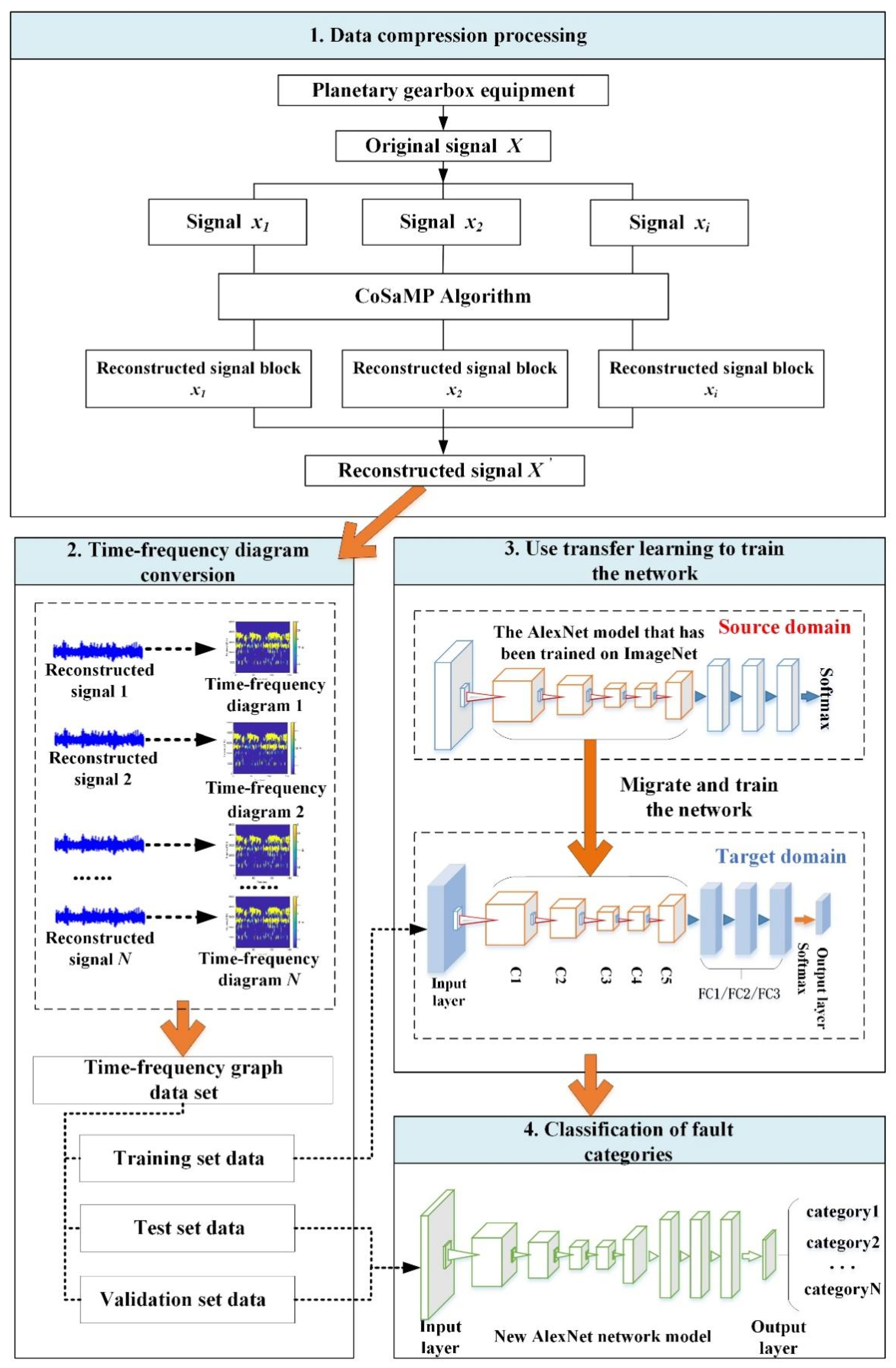
The framework flow of diagnosing faults utilizing deep transfer learning and compressed sensing is shown in Figure 4. The framework of the method mainly includes: data collection, data compression and reconstruction, time–frequency graph conversion, and the use of transfer learning to train the network, etc.
The specific implementation stages are presented as the following:
Step 1: Data collection. The vibration sensor is used to attain the original vibration signal x of the planetary gearbox.
Step 2: Data compression. The collected raw vibration signal x will be divided into xi signal blocks. Optimizing the dictionary Ψ by DCT to map signals into sparse transforms and the original signal x = Ψθ can obtain the sparse transformation signal θ. Sensing matrix A = ΦΨ (that is, observation matrix × sparse matrix) compresses the sparse signal data, and obtains the data compressed signal observation value y = Aθ.
Step 3: Signal reconstruction. Using the CoSaMP Reconstruction Algorithm, using the sensor matrix A1,..., Ai and compressed signal y1,...,yi to reconstruct, obtain the restored sparse signal θ1,…, θi. At the same time, perform an inverse sparse transformation to obtain reconstructed signal blocks x1,...,xi, and connect the reconstructed signal blocks one by one, and finally form a complete reconstructed signal x′.
Step 4: Time–frequency diagram conversion. Perform continuous wavelet transform on the reconstructed signal to obtain a time–frequency graph data set, and divide the dataset into three sections: training, test, and validation sets.
Step 5: Transfer learning. Use the pretrained AlexNet network model parameters of the source domain as the migration object. Using model fine-tuning, import the training set data, and retrain the fine-tuned model to obtain the deep transfer learning AlexNet network model.
Step 6: Classification of fault categories. Import the test set and verification set data into the trained deep transfer learning AlexNet network model and output the outcomes of the fault diagnosis.
5. The Verification of The Experimental Data
5.1. The Preparation of The Experiment
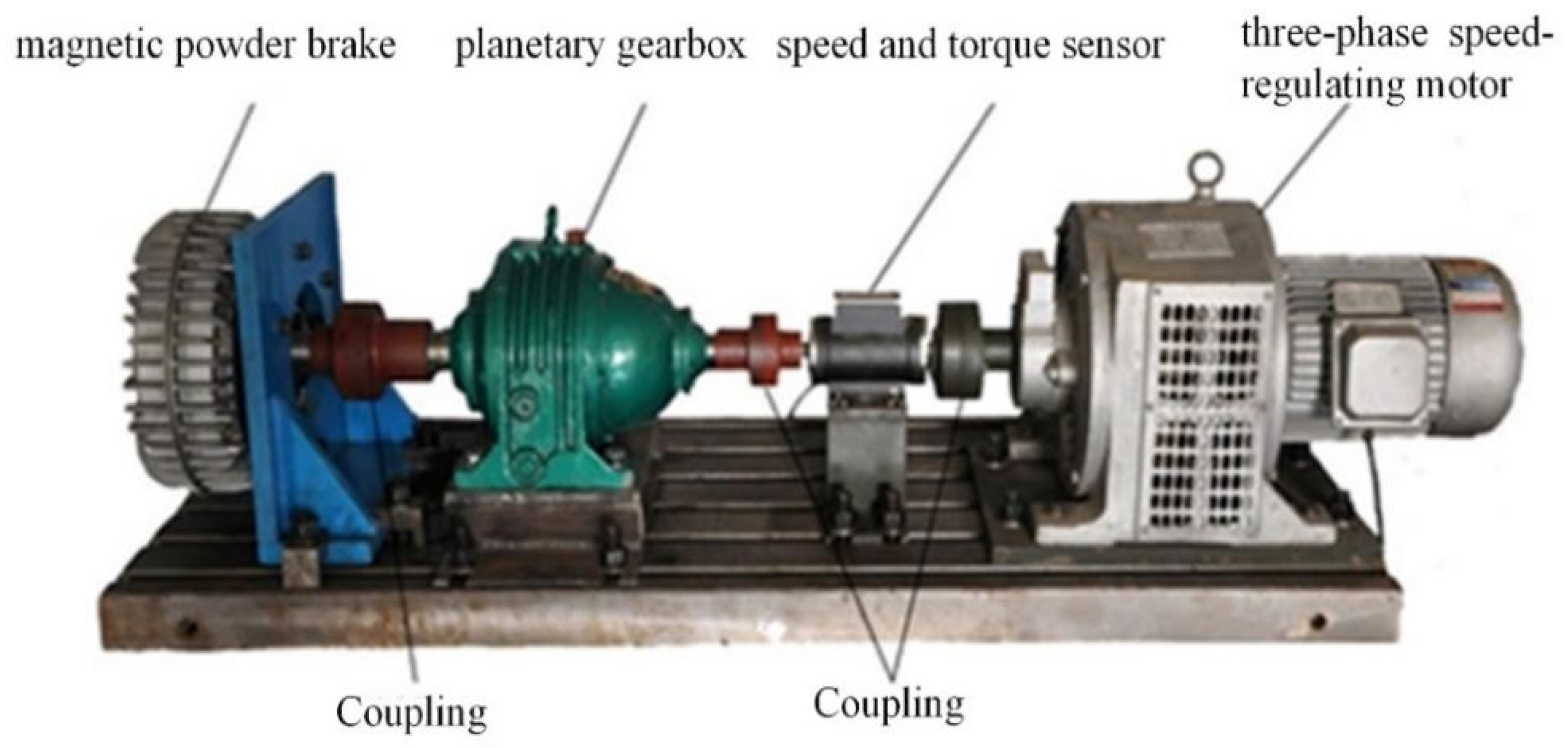
To validate the effectiveness of the method of diagnosing faults utilizing TL and the sense of compression proposed in the manuscript paper, Figure 5 depicts the established experimental platform of the planetary gearbox that is composed of a planetary gearbox, a three-phase speed-regulating motor, a sensor for speed and torque, and a magnetic powder brake.
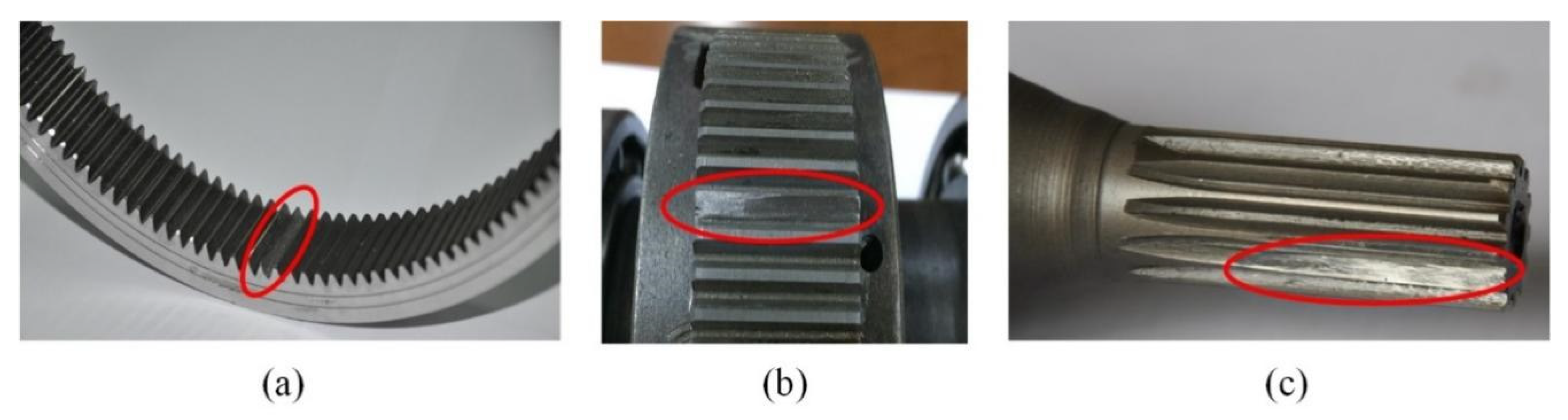
The experiment presets four states, namely, normal state, ring gear failure, planetary gear failure, and sun gear failure. The specific failures are shown in Figure 6. The experiment was carried out at 400 rpm, 800 rpm, and 1200 rpm. The magnetic powder brake was set with three loads of 0 Nm, 0.4 Nm, and 0.8 Nm for each speed. The frequency of the sampling is assigned to 20 kHz, and the collection time of the vibration signal for each sample is 12 s. In total, 30 groups of samples of vibration signals are collected in each working condition, and the vibration signals collected in the four states are shown in Table 1. In the data compression effect–evaluation index, CR (Compressing Ratio, CR) is used to represent the data compression rate, and the range is set to [0, 1]; MSE (Mean Square Error, MSE) is used to represent the standard mean square error index, which can be expressed by
In the Equation, M represents the compressed vibration signal and N represents the original vibration signal. As the CR increases, the compression ratio of the data also increases.
In the Equation, Z represents the original signal, and Z′ represents the reconstructed signal. The smaller the MSE value, the higher the accuracy of the data compression and reconstruction signal. When the data compression rate is larger, the MSE value is smaller, indicating that the data compression and reconstruction effect is better.
5.2. Data Preprocessing
To satisfy the requirement of the input data of the deep transfer learning AlexNet network model, the original vibration signal needs to be converted into a time–frequency graph. All the following experimental data are uniformly verified using four preset failure datasets whose speed is 1200 rpm, a load of 0.8 Nm, and 10 groups of samples’ working conditions. A cycle denoted by T = Fs/v = 20,000/(1200/60) = 1000 shows the number of sampling points. Therefore, the length of the sample is set to 3000 as the basis for generating the time–frequency graph. The size of the time–frequency diagram is set to 227 × 227, as shown in Figure 7. Additionally, using continuous wavelet transform, the four kinds of preset fault original signals are converted into corresponding time–frequency graph datasets, as shown in Table 2. Additionally, CR = 0.3, CR = 0.4, CR = 0.5, CR = 0.6, CR = 0.7, and CR = 0.8. The reconstructed signals under these six different compression ratios are converted into corresponding time–frequency diagrams, and the verification set is all 50 samples. To compare and analyze with traditional machine learning algorithms, the 3000 sampling points as sample data are used as the basis for extracting 20 characteristic parameters in a time domain and frequency domain (such as root mean square, variance, peak-to-peak value, etc.) [40,41], as shown in Table 3. The purpose is to verify that the trained deep transfer learning AlexNet network model is compared with the traditional machine learning algorithm under different compression rates to determine the appropriate compression rate for fault diagnosis.
5.3. Comparison and Analysis of Compression and Reconstruction Algorithms
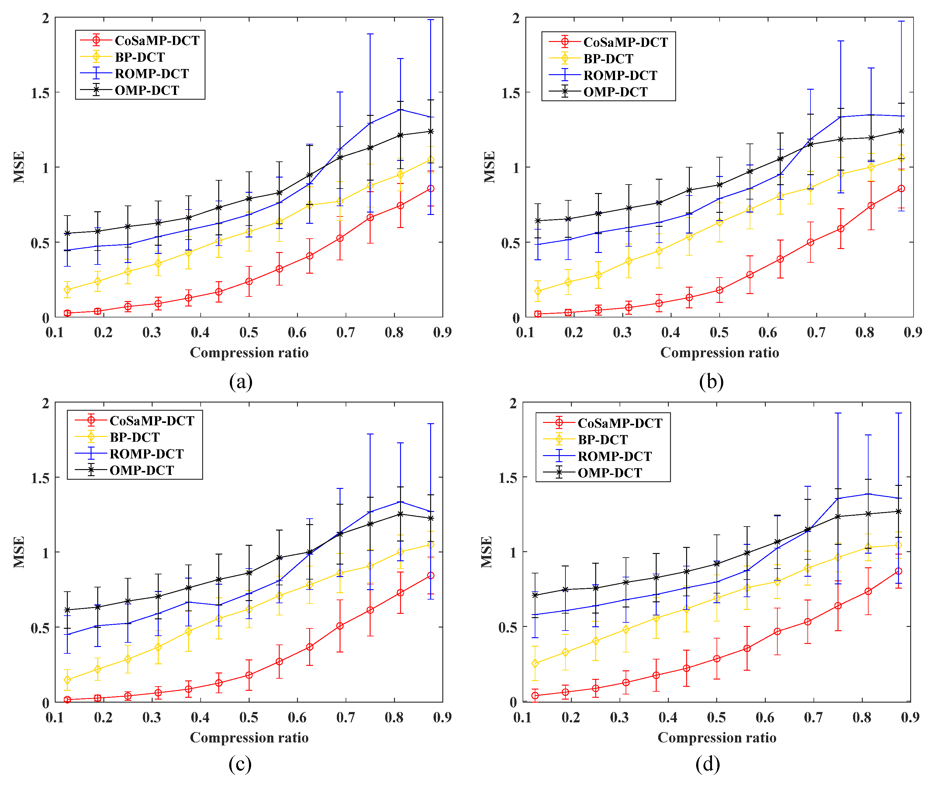
To validate the efficiency of the CoSaMP approach, a comprehensive analysis is carried out from the perspective of the influence of different compression ratio changes on the algorithm. The compression reconstruction algorithm was verified by using four preset fault data sets whose speed is assigned to 1200 rpm and 0.8 Nm loading. To assure the reconstruction outcome of the approach, the sparse dictionary matrix adopts the DCT generation method uniformly. Among them, 13 compression ratios are set for each dataset, and 100 experiments are performed for each compression ratio. Find the corresponding variance σ and average μ in Figure 8, which also shows the 95% confidence interval [μ − 2σ, μ + 2σ] method. Figure 8 presents the results of the analysis when CR < 0.6 and the MSE index of the CoSaMP reconstruction approach suggested in the manuscript is smaller than the others. The accuracy, superiority, and efficiency of the suggested approach are proven. When CR > 0.6, all reconstruction algorithms have larger variance values when the rate of compression is increased. Among them, the variance value of the ROMP algorithm is the most prominent, which proves that the higher the compression rate, the greater the MSE index, and the less ideal the data compression and reconstruction effect. Therefore, it is proven that when the compression ratio of the proposed method is set to 0.5, the more ideal the data reconstruction effect is, and the more suitable it is for data compression.
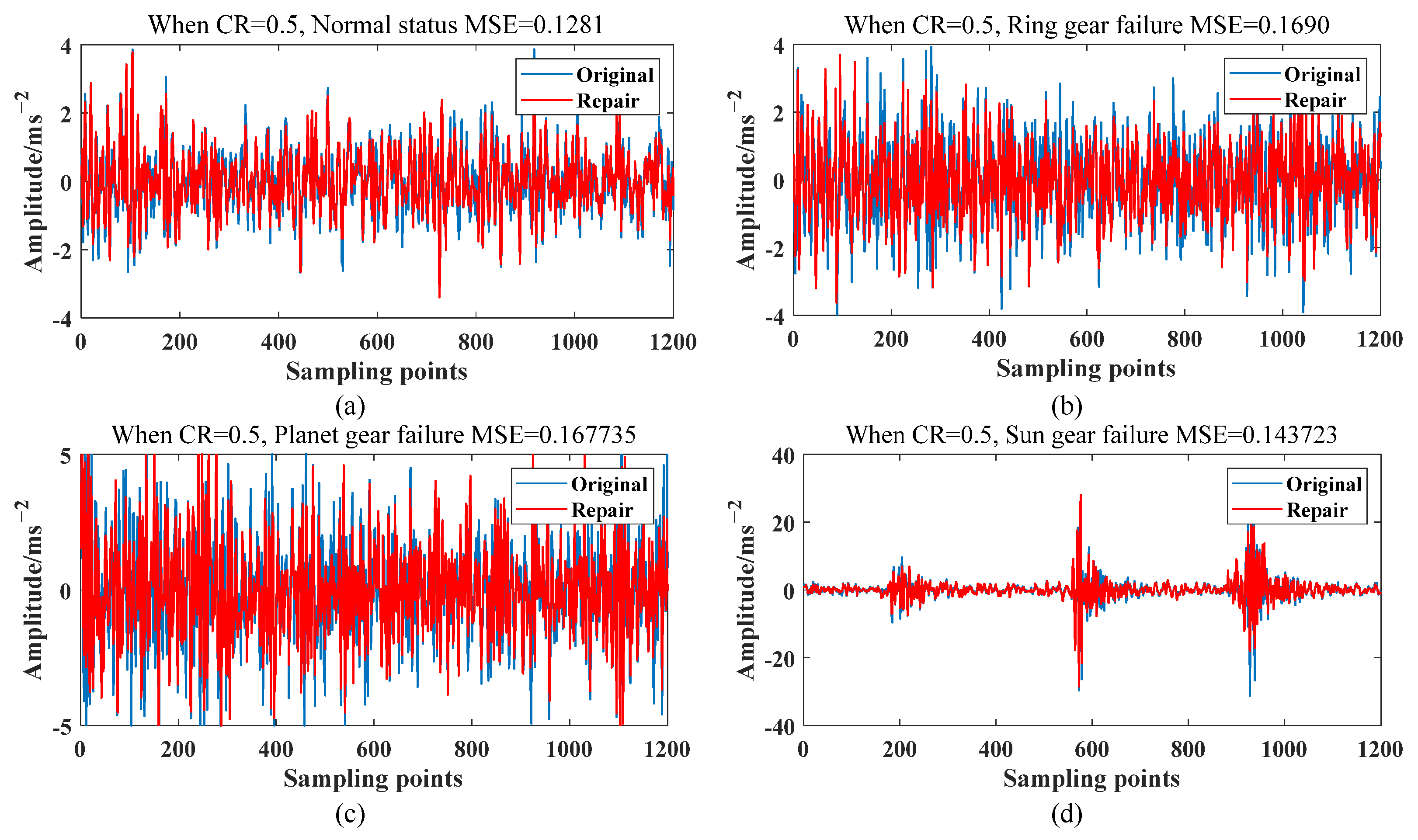
The four preset fault signal compression and reconstruction effects are shown in Figure 9, which further validate the efficiency of the CoSaMP algorithm when the compression ratio CR = 0.5 is set. The blue represents the original signal, and the red represents the reconstructed signal. Figure 9 presents the results of the analysis. The smaller the MSE index, the higher the reconstruction accuracy, indicating that under the same parameter-setting conditions, the reconstructed signal recovered by the proposed CoSaMP reconstruction algorithm is closer to the original signal, and it also proves that the data compression and reconstruction effect is better.
5.4. Comparative Analysis of Training Network and Diagnosis Results
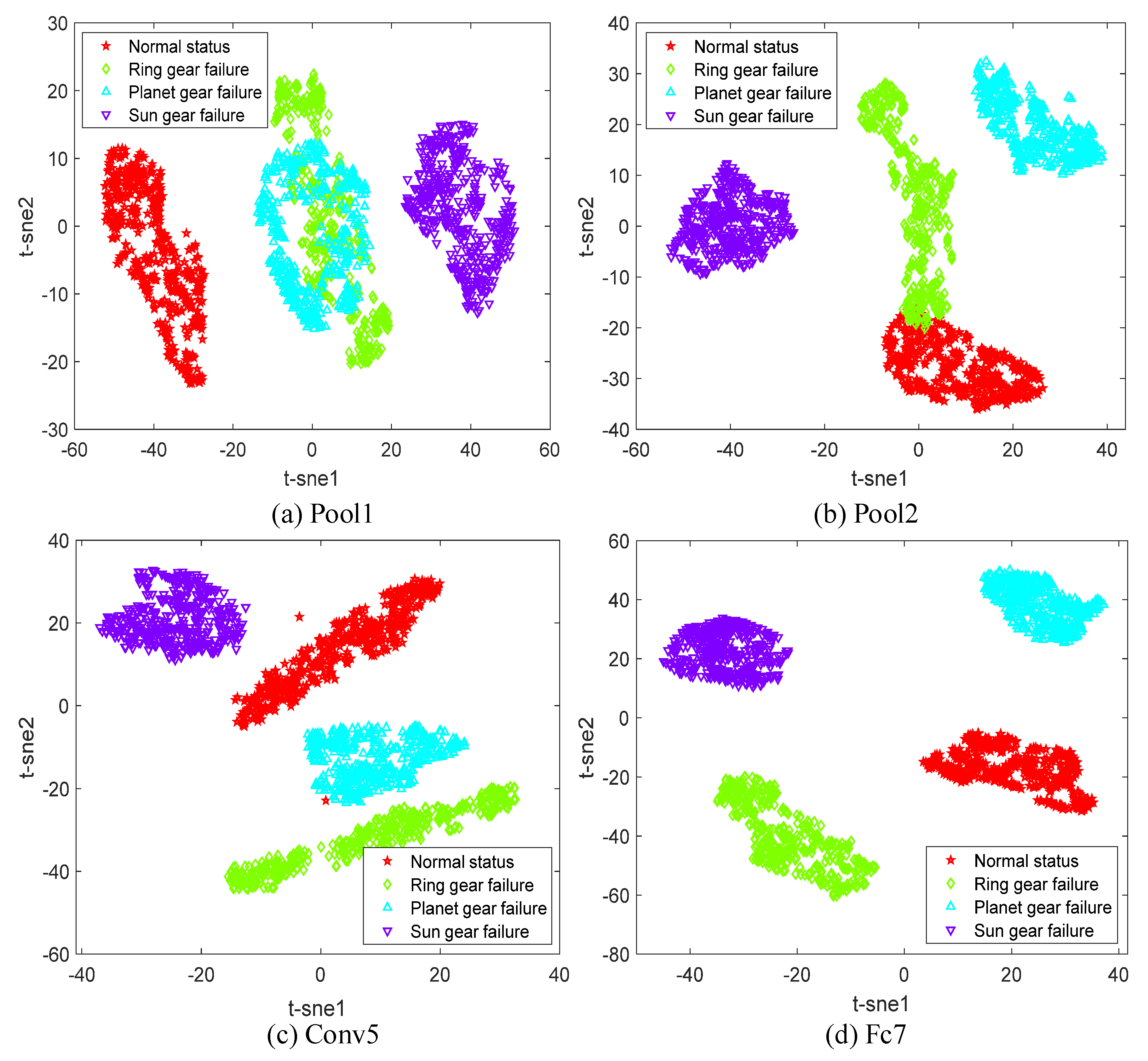
The important parameter settings of the deep transfer learning AlexNet network approach are presented in Table 4. To verify the effectiveness of the network model, the four preset fault original signal time–frequency graph datasets in Section 5.2 are used for verification. In total, 600 samples as a training fault set are contained in each set, and the test set contains 150 data points. time–To train and diagnose faults reaching an accuracy ratio of 100%, the original signal time–frequency graph dataset into the deep migration learning AlexNet network model is imported, as shown in Table 4. To further prove the ability of the AlexNet network model to derive features of the image and category recognition in the manuscript, t-distributed Stochastic Neighbor Embedding (t-SNE) [42] is employed for the image feature extraction process. Figure 10 shows the performance of data visualization analysis Figure 10a is the feature extracted by the first highest PL. The feature data intersect each other, and it is difficult to distinguish the fault state that can be seen; Figure 10b is the feature extracted by the second maximum pooling layer. It can be seen that there are still some data that are not distinguished; Figure 10c is the feature of the fifth CL (Conv5), and the four types of fault state data can be distinguished; Figure 10d is the feature of the second completely joined layer (FC7), which can distinguish the four failure states well, and has achieved a good data clustering effect. Therefore, the AlexNet network model employing deep transfer learning proposed in the manuscript can be proven and has robust feature derivation and classification abilities.
To further validate the precision of fault diagnosis of the trained deep transfer learning AlexNet network under different compression ratios, the verification sets under different compression ratios into the trained network were imported, and Table 5 summarizes the fault diagnosis outcomes. Compared with other compression rates, when CR = 0.8, the fault diagnosis accuracy of deep transfer learning AlexNet network model is only 25.69%. Among them, the fault types of ring gear and planetary gear cannot be identified, indicating that the higher the compression ratio, the lower the fault diagnosis accuracy. When CR ≤ 0.4, the fault diagnosis result reaches more than 98%, indicating that very critical fault features are included in the compressed signal. Among them, when CR = 0.3, it reaches 100.0% as the diagnostic result of the original signal. Experiments show that important information will not be lost in the process of data compression, so it can effectively improve the accuracy of fault diagnosis. When CR = 0.5, the diagnosis result reaches 97.78%. Even under high compression ratio, the important signal can still be retained in the compressed signal, so that a better diagnosis effect can be obtained, which is very suitable for fault diagnosis.
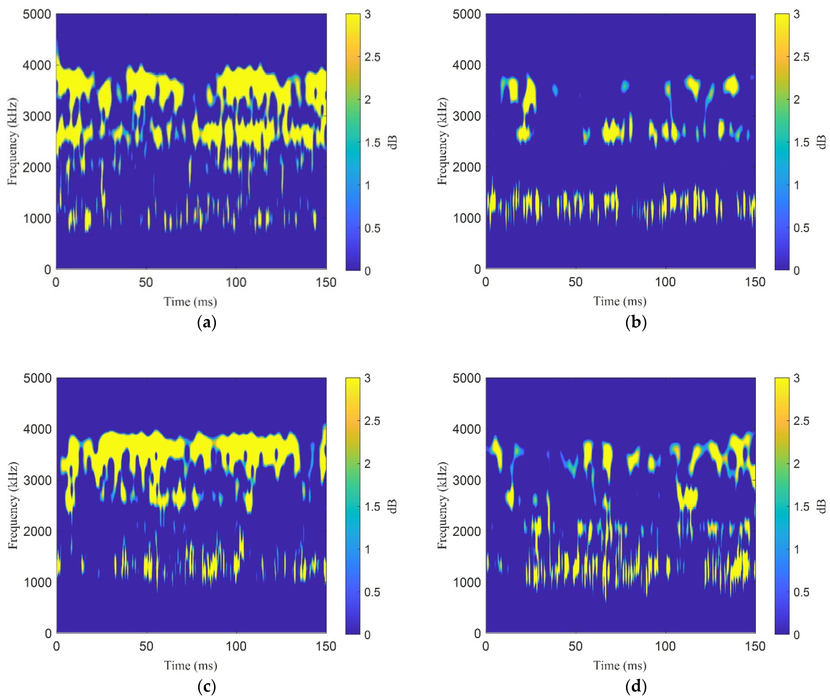
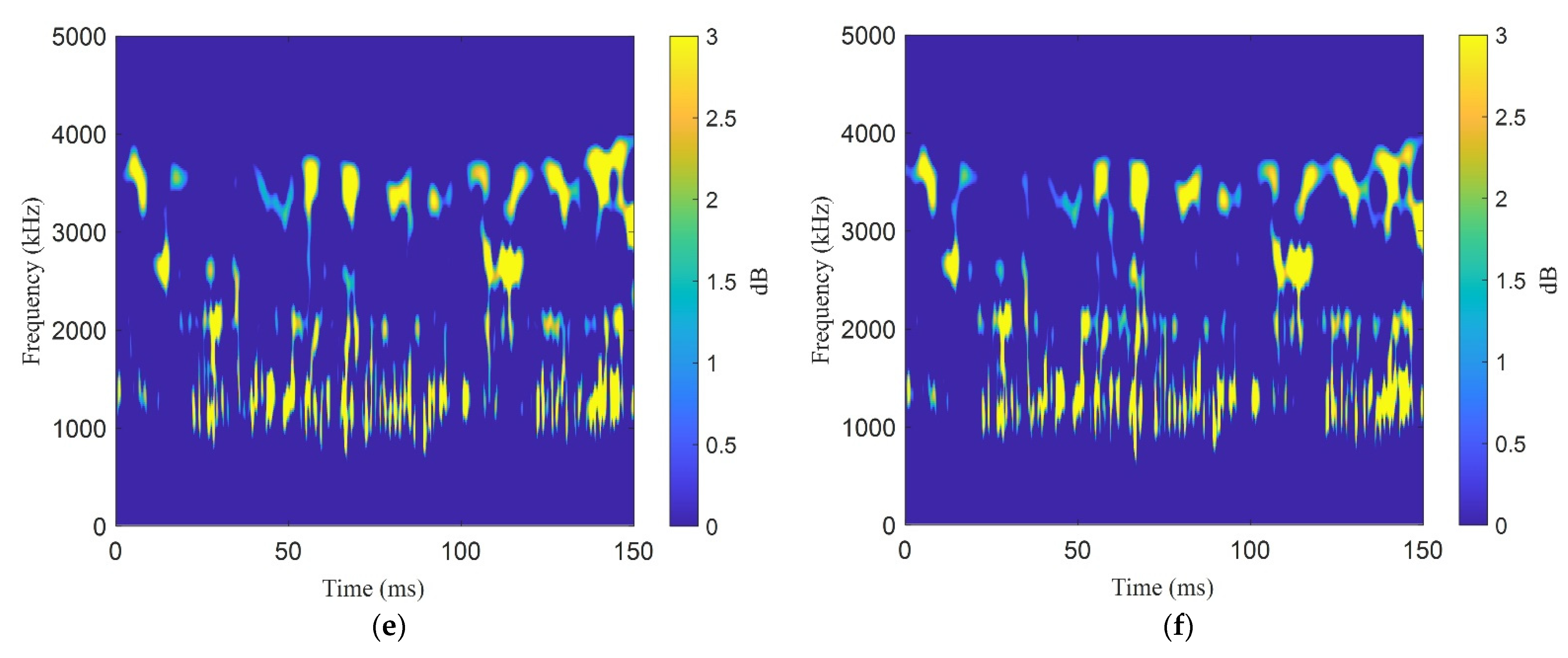
To further prove the impact of various compression rates on the classification accuracy of the deep migration learning AlexNet network model, Figure 11 depicts the time–frequency graph variation process of verified sun gear failures under various compression ratios. Figure 11a shows the time–frequency diagram characteristic of the original signal. Figure 11b shows that when CR = 0.8, it is easy to see that the time–frequency diagram of the compressed and reconstructed signal is quite different from the original signal. It shows that when the data compression rate is high, very important information is lost. As a result, the classification accuracy of the AlexNet network model is low. Figure 11c shows that when CR = 0.7, it can reflect the basic contour of the time–frequency diagram with the original signal, but it is not very obvious, and only 45.15% of them can be seen by observing the diagnostic results corresponding to Table 4. It means that the basic feature information has been included under the current compression rate, but the diagnosis accuracy is low. Figure 11d shows that when CR = 0.6, it can be clearly seen that it is similar to the time–frequency diagram of the original signal. However, there are still some interference signals which affect the accuracy of the diagnosis results. Figure 11e shows that when CR = 0.5, the time–frequency diagram of the compressed and reconstructed signal is very close to the original signal, and it shows that a large number of original signal features are retained in the compressed signal, which can effectively improve the classification accuracy of the AlexNet network model.
In summary, as the compression rate increases, the fault diagnosis accuracy rate gradually decreases. Assuming that the diagnostic accuracy rate is 97% acceptable, CR = 0.5 can greatly reduce the network requirements for massive data transmission. Therefore, it is hoped to obtain the best combination between fault diagnosis accuracy and network transmission.
5.5. Comparative Analysis of Different Network Models
To prove the effectiveness of the deep transfer learning AlexNet network model proposed in this article, one must compare and analyze with SqueezeNet, ResNet−18, GoogLeNet network model, as well as traditional machine learning SVM (Support Vector Machine, SVM) and RF (Random Forest, RF). Among them, in order to maintain the consistency of the data, the network model is uniformly verified with the time–frequency graph dataset in Section 5.2; The traditional machine learning is uniformly verified by the data set in Table 3, and the PCA (Principle Component Analysis, PCA) is uniformly used to reduce the dimension of fault features.
It can be seen from Table 6 that when CR = 0.5, the precision of the AlexNet network model is 97.78% and when the comparison is conducted among the other three network models, the accuracy rate is higher and the execution time is the shortest. Among them, the accuracy of the ResNet−18 network model is only 76.38%. Under the same compression rate, the diagnostic results of traditional machine learning SVM and RF are 92.23% and 90.80%, respectively. Compared with the network model of AlexNet, the running time of traditional machine learning is longer, and its diagnostic accuracy is also lower than that of the network model of AlexNet. The results show that, compared with traditional machine learning algorithms, the AlexNet network model has obvious advantages in accuracy and speed.
It can be seen from Table 7 that when CR = 0.6, the accuracy of the AlexNet network model is 79.86%. The accuracy rate is still higher than the other three models, which effectively proves that the network model has the advantage of strong fault–feature extraction ability. Compared with the traditional machine learning algorithm, the AlexNet network model has a better diagnosis effect under the same compression rate, and the diagnosis time is also shorter. This effectively proves the validity and feasibility of the AlexNet network model.
It can be seen from Table 8 that when CR = 0.8, Not only the accuracy rates of the four network models are less than 56%, but also the diagnostic accuracy of traditional machine learning algorithms is less than 30%. The results show that with the increase in the compression rate, the diagnostic results of the traditional machine learning method and the four network models all show a downward trend. This effectively proves that the higher the data compression rate, the less key information it contains, and the less accurate the reconstruction will be. Therefore, this compression ratio is not suitable for use in troubleshooting.
In summary, although the ResNet−18 and GoogLeNet network models are compared to the AlexNet network models, AlexNet has stronger network learning and image classification capabilities, but requires a lot of sample data and computing time during the training process. Too many network layers are prone to excessive feature extraction, which leads to overfitting. Compared with traditional machine learning algorithms, the AlexNet network model has faster computing speed and higher diagnostic accuracy. Therefore, it can be seen from the results and running time of fault diagnosis that the AlexNet network model is more suitable for fault diagnosis of vibration signals.
6. Conclusions
This paper proposes a method for diagnosing faults using transfer learning and compressed sensing theory, which combines the continuous wavelet transform and the AlexNet convolutional neural network. The following are the main conclusions:
The original vibration signal is compressed and reconstructed using the CoSaMP reconstruction algorithm, and the experiment shows that a good compression effect is obtained. The continuous wavelet transform is used to convert the compressed signal into a time–frequency graph, reducing feature extraction complexity.
A deep migration learning model for planetary gearbox fault detection was developed. Five convolutional layers from a pretrained AlexNet network model as the migration target was selected. The model has robust feature extraction and fault classification capabilities. The fault diagnosis accuracy rate reaches 97.78 percent when the compression ratio CR = 0.5. The deep transfer learning AlexNet network model outperforms the SqueezeNet, ResNet−18, and GoogLeNet network models regarding classification accuracy and robustness. A specific reference value is provided to diagnose faults in rotating machinery and has a promising future application.
Author Contributions
Data curation, H.B. and H.Y.; Resources, L.W. and X.Z.; Supervision, X.J.; Validation, L.W. and X.J.; Writing—original draft, H.B.; Writing—review & editing, H.B. All authors have read and agreed to the published version of the manuscript.
Funding
This study did not receive any funding.
Data Availability Statement
Data will be provided upon request to the authors.
Conflicts of Interest
The authors declare that they have no conflict of interest.
References
- Ye, S.; Zhang, J.; Xu, B.; Zhu, S.; Xiang, J.; Tang, H. Theoretical investigation of the contributions of the excitation forces to the vibration of an axial piston pump. Mech. Syst. Signal Process. 2019, 129, 201–217. [Google Scholar] [CrossRef]
- Pei, X.; Zheng, X.; Wu, J. Intelligent bearing fault diagnosis based on Teager energy operator demodulation and multiscale compressed sensing deep autoencoder. Measurement 2021, 179, 109452. [Google Scholar] [CrossRef]
- Xia, M.; Shao, H.; Williams, D.; Lu, S.; Shu, L.; de Silva, C.W. Intelligent fault diagnosis of machinery using digital twin-assisted deep transfer learning. Reliab. Eng. Syst. Saf. 2021, 215, 107938. [Google Scholar] [CrossRef]
- Liang, J.; Xiao, D.; Wang, M.; Li, M.; Liu, R. Low-complexity privacy preserving scheme based on compressed sensing and non-negative matrix factorization for image data. Opt. Lasers Eng. 2020, 129, 106056. [Google Scholar] [CrossRef]
- Saufi, S.R.; Ahmad, Z.A.B.; Leong, M.S.; Lim, M.H. Gearbox fault diagnosis using a deep learning model with limited data sample. IEEE Trans. Ind. Inform. 2020, 16, 6263–6271. [Google Scholar] [CrossRef]
- Lu, F.; Cao, Z.; Xie, Y.; Xu, L. Precise wide-band electrical impedance spectroscopy measurement via an ADC operated below the Nyquist sampling rate. Measurement 2021, 174, 108995. [Google Scholar] [CrossRef]
- Chen, J.; Xu, B.; Zhang, X. A Vibration Feature Extraction Method Based on Time-Domain Dimensional Parameters and Mahalanobis Distance. Math. Probl. Eng. 2021, 2021, 2498178. [Google Scholar] [CrossRef]
- Ke, W.; Hao, C. Research on radar main lobe false target jamming feature extraction based on time-frequency domain and fluctuation characteristics. J. Phys. Conf. Ser. 2021, 1871, 012079. [Google Scholar]
- Rigatos, G.; Siano, P. Power transformers’ condition monitoring using neural modeling and the local statistical approach to fault diagnosis. Int. J. Electr. Power Energy Syst. 2016, 80, 150–159. [Google Scholar] [CrossRef]
- Du, W.-T.; Zeng, Q.; Shao, Y.-M.; Wang, L.-M.; Ding, X.-X. Multi-Scale Demodulation for Fault Diagnosis Based on a Weighted-EMD De-Noising Technique and Time—Frequency Envelope Analysis. Appl. Sci. 2020, 10, 7796. [Google Scholar] [CrossRef]
- Zhao, X.; Bao, H.; Tian, L.; Yuan, Y.; Dai, J. Research on the Application of Rolling Bearing Fault Diagnosis Based on Order Cepstrum Analysis. In Proceedings of the 2016 7th International Conference on Mechatronics, Control and Materials (ICMCM 2016), Changsha, China, 29–30 October 2016; Atlantis Press: Changsha, China, 2016; pp. 93–96. [Google Scholar]
- Fei, S.-W. The Hybrid Method of VMD-PSR-SVD and Improved Binary PSO-KNN for Fault Diagnosis of Bearing. Shock Vib. 2019, 2019, 4954920. [Google Scholar] [CrossRef] [Green Version]
- Lei, Y.; Jiang, W.; Niu, H.; Shi, X.; Yang, X. Fault Diagnosis of Axial Piston Pump Based on Extreme-Point Symmetric Mode Decomposition and Random Forests. Shock. Vib. 2021, 2021, 6649603. [Google Scholar]
- Lv, X.; Wang, H.; Zhang, X.; Liu, Y.; Jiang, D.; Wei, B. An evolutional SVM method based on incremental algorithm and simulated indicator diagrams for fault diagnosis in sucker rod pumping systems. J. Pet. Sci. Eng. 2021, 203, 108806. [Google Scholar] [CrossRef]
- Shao, K.; Fu, W.; Tan, J.; Wang, K. Coordinated approach fusing time-shift multiscale dispersion entropy and vibrational Harris hawks optimization-based SVM for fault diagnosis of rolling bearing. Measurement 2020, 173, 108580. [Google Scholar] [CrossRef]
- Zhang, X.; Li, C.; Wang, X.; Wu, H. A novel fault diagnosis procedure based on improved symplectic geometry mode decomposition and optimized SVM. Measurement 2021, 173, 108644. [Google Scholar] [CrossRef]
- Liu, Y.; Ding, K.; Zhang, J.; Li, Y.; Yang, Z.; Zheng, W.; Chen, X. Fault diagnosis approach for photovoltaic array based on the stacked auto-encoder and clustering with IV curves. Energy Convers. Manag. 2021, 245, 114603. [Google Scholar] [CrossRef]
- Huang, T.; Fu, S.; Feng, H.; Kuang, J. Bearing fault diagnosis based on shallow multi-scale convolutional neural network with attention. Energies 2019, 12, 3937. [Google Scholar] [CrossRef] [Green Version]
- Xing, T.; Shen, J.; Meng, Z. Fault Diagnosis of Marine Wind Turbine Gearbox Based on New Technology of Compressed Sensing. J. Coast. Res. 2020, 104, 406–409. [Google Scholar] [CrossRef]
- Shi, P.; Guo, X.; Han, D.; Fu, R. A sparse auto-encoder method based on compressed sensing and wavelet packet energy entropy for rolling bearing intelligent fault diagnosis. J. Mech. Sci. Technol. 2020, 34, 1445–1458. [Google Scholar] [CrossRef]
- Shao, H.; Jiang, H.; Zhang, H.; Duan, W.; Liang, T.; Wu, S. Rolling bearing fault feature learning using improved convolutional deep belief network with compressed sensing. Mech. Syst. Signal Process. 2018, 100, 743–765. [Google Scholar] [CrossRef]
- Shi, P.; Ma, X.; Han, D. A weak fault diagnosis method for rotating machinery based on compressed sensing and stochastic resonance. J. Vibroeng. 2019, 21, 654–664. [Google Scholar] [CrossRef]
- Liu, C.; Cheng, G.; Chen, X.; Pang, Y. Planetary gears feature extraction and fault diagnosis method based on VMD and CNN. Sensors 2018, 18, 1523. [Google Scholar] [CrossRef] [PubMed] [Green Version]
- Li, H.P.; Qi, Z.L.; Hu, J.P.; Zhang, X.Y. Research on the Method of Rotary Machinery Fault Diagnosis based on PCA and DBN. IOP Conf. Ser. Mater. Sci. Eng. 2021, 1043, 022044. [Google Scholar] [CrossRef]
- Tang, Z.; Bo, L.; Liu, X.; Wei, D. A semi-supervised transferable LSTM with feature evaluation for fault diagnosis of rotating machinery. Appl. Intell. 2021, 52, 1703–1717. [Google Scholar] [CrossRef]
- Wang, H.; Liu, C.; Jiang, D.; Jiang, Z. Collaborative deep learning framework for fault diagnosis in distributed complex systems. Mech. Syst. Signal Process. 2021, 156, 107650. [Google Scholar] [CrossRef]
- Ahmadi, A.; Kashefi, M.; Shahrokhi, H.; Nazari, M.A. Computer aided diagnosis system using deep convolutional neural networks for ADHD subtypes. Biomed. Signal Process. Control 2020, 63, 102227. [Google Scholar] [CrossRef]
- Barcelos, A.S.; Cardoso, A.J.M. Current-based bearing fault diagnosis using deep learning algorithms. Energies 2021, 14, 2509. [Google Scholar] [CrossRef]
- He, J.; Li, X.; Chen, Y.; Chen, D.; Guo, J.; Zhou, Y. Deep Transfer Learning Method Based on 1D-CNN for Bearing Fault Diagnosis. Shock Vib. 2021, 2021, 6687331. [Google Scholar] [CrossRef]
- Xu, Y.; Li, Z.; Wang, S.; Li, W.; Sarkodie-Gyan, T.; Feng, S. A hybrid deep-learning model for fault diagnosis of rolling bearings. Measurement 2020, 169, 108502. [Google Scholar] [CrossRef]
- Xin, Y.; Li, S.; Wang, J.; An, Z.; Zhang, W. Intelligent fault diagnosis method for rotating machinery based on vibration signal analysis and hybrid multi-object deep CNN. IET Sci. Meas. Technol. 2020, 14, 407–415. [Google Scholar] [CrossRef]
- Zhao, B.; Zhang, X.; Li, H.; Yang, Z. Intelligent fault diagnosis of rolling bearings based on normalized CNN considering data imbalance and variable working conditions. Knowl. Based Syst. 2020, 199, 105971. [Google Scholar] [CrossRef]
- Ramteke, D.S.; Pachori, R.B.; Parey, A. Automated Gearbox Fault Diagnosis Using Entropy-Based Features in Flexible Analytic Wavelet Transform (FAWT) Domain. J. Vib. Eng. Technol. 2021, 9, 1703–1713. [Google Scholar] [CrossRef]
- Donoho, D.L. Compressed sensing. IEEE Trans. Inf. Theory 2006, 52, 1289–1306. [Google Scholar] [CrossRef]
- Needell, D.; Troppb, J.A. CoSaMP: Iterative signal recovery from incomplete and inaccurate samples—ScienceDirect. Appl. Comput. Harmon. Anal. 2009, 26, 301–321. [Google Scholar] [CrossRef] [Green Version]
- Jin, T.; Yan, C.; Chen, C.; Yang, Z.; Tian, H.; Wang, S. Light neural network with fewer parameters based on CNN for fault diagnosis of rotating machinery. Measurement 2021, 181, 109639. [Google Scholar] [CrossRef]
- Yu, Y.; Guo, L.; Tan, Y.; Gao, H.; Zhang, J. Multi-source Partial Transfer Network for Machinery Fault Diagnostics. IEEE Trans. Ind. Electron. 2021, 69, 10585–10594. [Google Scholar] [CrossRef]
- Liu, Y.Z.; Shi, K.M.; Li, Z.X.; Ding, G.F.; Zou, Y.S. Transfer learning method for bearing fault diagnosis based on fully convolutional conditional Wasserstein adversarial Networks. Measurement 2021, 180, 109553. [Google Scholar] [CrossRef]
- Ullah, I.; Khan, R.U.; Yang, F.; Wuttisittikulkij, L. Deep learning image-based defect detection in high voltage electrical equipment. Energies 2020, 13, 392. [Google Scholar] [CrossRef] [Green Version]
- Samuel, P.D.; Pines, D.J. A review of vibration-based techniques for helicopter transmission diagnostics. J. Sound Vib. 2005, 282, 475–508. [Google Scholar] [CrossRef]
- Liu, Z.; Qu, J.; Zuo, M.J.; Xu, H.-B. Fault level diagnosis for planetary gearboxes using hybrid kernel feature selection and kernel Fisher discriminant analysis. Int. J. Adv. Manuf. Technol. 2012, 67, 1217–1230. [Google Scholar] [CrossRef]
- Jiang, W.; Zhou, J.; Liu, H.; Shan, Y. A multi-step progressive fault diagnosis method for rolling element bearing based on energy entropy theory and hybrid ensemble auto-encoder. ISA Trans. 2019, 87, 235–250. [Google Scholar] [CrossRef] [PubMed]
Figure 1.
Diagram of traditional compression and compressed sensing data acquisition: (a) traditional compression process; (b) compressed sensing process.
Figure 1.
Diagram of traditional compression and compressed sensing data acquisition: (a) traditional compression process; (b) compressed sensing process.

Figure 2.
AlexNet network model structure diagram.

Figure 3.
Schematic diagram of transfer learning method based on network model.

Figure 4.
Process of fault diagnosis method based on deep transfer learning and compressed sensing.

Figure 5.
Schematic diagram of the planetary gearbox experimental platform.

Figure 6.
Schematic diagram of gear preset fault: (a) ring gear fault; (b) planet gear fault; (c) sun gear fault.
Figure 6.
Schematic diagram of gear preset fault: (a) ring gear fault; (b) planet gear fault; (c) sun gear fault.

Figure 7.
Schematic diagram of wavelet transform of original signal under four fault states: (a) normal status; (b) ring gear; (c) planet gear; and (d) sun gear.
Figure 7.
Schematic diagram of wavelet transform of original signal under four fault states: (a) normal status; (b) ring gear; (c) planet gear; and (d) sun gear.

Figure 8.
Compare and analyze the 95% confidence interval of MES on the four datasets with other compression reconstruction algorithms: (a) normal status, (b) ring gear, (c) planet gear, and (d) sun gear.
Figure 8.
Compare and analyze the 95% confidence interval of MES on the four datasets with other compression reconstruction algorithms: (a) normal status, (b) ring gear, (c) planet gear, and (d) sun gear.

Figure 9.
When CR = 0.5, compression and reconstruction analysis of four preset failures: (a) normal state (MSE = 0.1281), (b) ring gear failure (MSE = 0.1690), (c) planetary gear failure (MSE = 0.167735), (d) sun gear failure (MSE = 0.143723).
Figure 9.
When CR = 0.5, compression and reconstruction analysis of four preset failures: (a) normal state (MSE = 0.1281), (b) ring gear failure (MSE = 0.1690), (c) planetary gear failure (MSE = 0.167735), (d) sun gear failure (MSE = 0.143723).

Figure 10.
The t-SNE visual analysis of the AlexNet network feature extraction process: (a) maximum pooling layer 1 feature; (b) maximum pooling layer 2 feature; (c) Conv5 layer feature; (d) Fc7 layer feature.
Figure 10.
The t-SNE visual analysis of the AlexNet network feature extraction process: (a) maximum pooling layer 1 feature; (b) maximum pooling layer 2 feature; (c) Conv5 layer feature; (d) Fc7 layer feature.

Figure 11.
Schematic diagram of wavelet transform of sun gear fault under different compression ratios: (a) original signal; (b) CR = 0.8; (c) CR = 0.7; (d) CR = 0.6; (e) CR = 0.5; (f) CR = 0.4.
Figure 11.
Schematic diagram of wavelet transform of sun gear fault under different compression ratios: (a) original signal; (b) CR = 0.8; (c) CR = 0.7; (d) CR = 0.6; (e) CR = 0.5; (f) CR = 0.4.


Table 1.
Four preset fault datasets under different working conditions.
| Signal State | Speed (rmp) | Load (Nm) | Sampling Frequency | Sampling Time | Number of Samples |
|---|---|---|---|---|---|
| Normal status | 400 | 0 | 20 kHz | 12 s | 30 groups |
| 800 | 0.4 | 20 kHz | 12 s | 30 groups | |
| 1200 | 0.8 | 20 kHz | 12 s | 30 groups | |
| Ring gear failure | 400 | 0 | 20 kHz | 12 s | 30 groups |
| 800 | 0.4 | 20 kHz | 12 s | 30 groups | |
| 1200 | 0.8 | 20 kHz | 12 s | 30 groups | |
| Planet gear failure | 400 | 0 | 20 kHz | 12 s | 30 groups |
| 800 | 0.4 | 20 kHz | 12 s | 30 groups | |
| 1200 | 0.8 | 20 kHz | 12 s | 30 groups | |
| Sun gear failure | 400 | 0 | 20 kHz | 12 s | 30 groups |
| 800 | 0.4 | 20 kHz | 12 s | 30 groups | |
| 1200 | 0.8 | 20 kHz | 12 s | 30 groups |
Table 2.
Four kinds of preset fault original signal time–frequency graph data set.
| Signal State | Total Sample | Training Samples | Test Sample | Validation Sample |
|---|---|---|---|---|
| Normal status | 800 | 600 | 150 | 50 |
| Ring gear failure | 800 | 600 | 150 | 50 |
| Planet gear failure | 800 | 600 | 150 | 50 |
| Sun gear failure | 800 | 600 | 150 | 50 |
| Total | 3200 | 2400 | 600 | 200 |
Table 3.
Four preset fault characteristic parameter datasets.
| Signal State | Total Sample | Training Samples | Test Sample | Validation Sample |
|---|---|---|---|---|
| Normal status | 800 | 20 × 600 | 20 × 150 | 20 × 50 |
| Ring gear failure | 800 | 20 × 600 | 20 × 150 | 20 × 50 |
| Planet gear failure | 800 | 20 × 600 | 20 × 150 | 20 × 50 |
| Sun gear failure | 800 | 20 × 600 | 20 × 150 | 20 × 50 |
| Total | 3200 | 2400 | 600 | 200 |
Table 4.
AlexNet network model parameter settings.
| Network Layer | Enter | Output | Activation Function |
|---|---|---|---|
| Input layer | 227 × 227 × 3 | / | / |
| Convolutional layer 1 | 227 × 227 × 3 | 55 × 55 × 96 | ReLU |
| Pooling layer 1 | 55 × 55 × 96 | 27 × 27 × 96 | / |
| Convolutional layer 2 | 27 × 27 × 96 | 27 × 27 × 256 | ReLU |
| Pooling layer 2 | 27 × 27 × 256 | 13 × 13 × 256 | / |
| Convolutional layer 3 | 13 × 13 × 256 | 13 × 13 × 384 | ReLU |
| Convolutional layer 4 | 13 × 13 × 384 | 13 × 13 × 384 | ReLU |
| Convolutional layer 5 | 13 × 13 × 384 | 13 × 13 × 256 | ReLU |
| Pooling layer 5 | 13 × 13 × 256 | 6 × 6 × 256 | / |
| Fully connected layer 1 | 6 × 6 × 256 | 512 | ReLU |
| Fully connected layer 2 | 512 | 256 | ReLU |
| Fully connected layer 3 | 256 | 4 | / |
| Output layer | / | 4 | / |
Table 5.
Analysis of the results of the AlexNet diagnosis method under different compression ratios.
Table 5.
Analysis of the results of the AlexNet diagnosis method under different compression ratios.
| Compression Ratio | Fault State | Total Accuracy | Execution Time | |||
|---|---|---|---|---|---|---|
| Normal Status | Ring Gear Failure | Planet Gear Failure | Sun Gear Failure | |||
| Original data | 100.0% | 100.0% | 100.0% | 100.0% | 100.0% | 1.256 s |
| CR = 0.3 | 100.0% | 100.0% | 100.0% | 100.0% | 100.0% | 1.201 s |
| CR = 0.4 | 100.0% | 94.40% | 100.0% | 100.0% | 98.60% | 1.238 s |
| CR = 0.5 | 100.0% | 91.10% | 100.0% | 100.0% | 97.78% | 1.263 s |
| CR = 0.6 | 94.40% | 47.20% | 77.80% | 100.0% | 79.85% | 1.226 s |
| CR = 0.7 | 66.70% | 13.90% | 0.00% | 100.0% | 45.15% | 1.669 s |
| CR = 0.8 | 2.80% | 0.00% | 0.00% | 100.0% | 25.70% | 1.773 s |
Table 6.
Comparative analysis of fault diagnosis between different network models and traditional methods when CR = 0.5.
Table 6.
Comparative analysis of fault diagnosis between different network models and traditional methods when CR = 0.5.
| Fault State | Different Network Models | Traditional Machine Learning | ||||
|---|---|---|---|---|---|---|
| Alexnet | SqueezeNet | ResNet−18 | GoogLeNet | SVM | RF | |
| Normal status | 100.0% | 94.40% | 100.0% | 97.20% | 95.50% | 93.00% |
| Ring gear failure | 91.10% | 91.70% | 8.30% | 55.60% | 86.20% | 82.10% |
| Planet gear failure | 100.0% | 97.20% | 97.20% | 100.0% | 91.70% | 95.50% |
| Sun gear failure | 100.0% | 100.0% | 100.0% | 100.0% | 95.50% | 92.60% |
| Total accuracy | 97.78% | 95.83% | 76.38% | 88.20% | 92.23% | 90.80% |
| Execution time | 1.359 s | 2.265 s | 3.406 s | 2.744 s | 11.037 s | 9.523 s |
Table 7.
Comparative analysis of fault diagnosis between different network models and traditional methods when CR = 0.6.
Table 7.
Comparative analysis of fault diagnosis between different network models and traditional methods when CR = 0.6.
| Fault State | Different Network Models | Traditional Machine Learning | ||||
|---|---|---|---|---|---|---|
| Alexnet | SqueezeNet | ResNet−18 | GoogLeNet | SVM | RF | |
| Normal status | 94.40% | 82.10% | 82.10% | 71.40% | 73.50% | 70.20% |
| Ring gear failure | 47.20% | 82.10% | 0.00% | 35.70% | 57.00% | 56.50% |
| Planet gear failure | 77.80% | 39.30% | 75.0% | 96.40% | 52.70% | 64.60% |
| Sun gear failure | 100.0% | 100.0% | 100.0% | 100.0% | 78.20% | 53.00% |
| Total accuracy | 79.85% | 75.89% | 64.28% | 75.89% | 65.35% | 61.08% |
| Execution time | 1.226 s | 2.089 s | 2.452 s | 2.348 s | 10.514 s | 10.171 s |
Table 8.
Comparative analysis of fault diagnosis between different network models and traditional methods when CR = 0.8.
Table 8.
Comparative analysis of fault diagnosis between different network models and traditional methods when CR = 0.8.
| Fault State | Different Network Models | Traditional Machine Learning | ||||
|---|---|---|---|---|---|---|
| AlexNet | SqueezeNet | ResNet−18 | GoogLeNet | SVM | RF | |
| Normal status | 28.00% | 69.40% | 35.70% | 82.10% | 33.30% | 28.50% |
| Ring gear failure | 0.00% | 33.30% | 0.00% | 10.70% | 26.50% | 22.00% |
| Planet gear failure | 0.00% | 0.00% | 0.00% | 28.60% | 31.00% | 26.40% |
| Sun gear failure | 100.0% | 100.0% | 100.0% | 100.0% | 24.20% | 21.70% |
| Total accuracy | 25.70% | 50.69% | 33.92% | 55.35% | 28.75% | 24.65% |
| Execution time | 1.773 s | 2.329 s | 4.262 s | 2.634 s | 10.832 s | 9.851 s |
Publisher’s Note: MDPI stays neutral with regard to jurisdictional claims in published maps and institutional affiliations. |
© 2022 by the authors. Licensee MDPI, Basel, Switzerland. This article is an open access article distributed under the terms and conditions of the Creative Commons Attribution (CC BY) license (https://creativecommons.org/licenses/by/4.0/).
Share and Cite
MDPI and ACS Style
Bai, H.; Yan, H.; Zhan, X.; Wen, L.; Jia, X. Fault Diagnosis Method of Planetary Gearbox Based on Compressed Sensing and Transfer Learning. Electronics 2022, 11, 1708. https://doi.org/10.3390/electronics11111708
AMA Style
Bai H, Yan H, Zhan X, Wen L, Jia X. Fault Diagnosis Method of Planetary Gearbox Based on Compressed Sensing and Transfer Learning. Electronics. 2022; 11(11):1708. https://doi.org/10.3390/electronics11111708
Chicago/Turabian StyleBai, Huajun, Hao Yan, Xianbiao Zhan, Liang Wen, and Xisheng Jia. 2022. "Fault Diagnosis Method of Planetary Gearbox Based on Compressed Sensing and Transfer Learning" Electronics 11, no. 11: 1708. https://doi.org/10.3390/electronics11111708
Note that from the first issue of 2016, this journal uses article numbers instead of page numbers. See further details here.