


Highlights
Please indicate how your work links to systems science via your contributions to systems practice, theory, and/or methodology.
- This study develops an auditable decision-support method for reproducing committee-assigned pharmaceutical supplier profiles from operational records. Supplier-grouped evaluation prevents repeated supplier identities from crossing training and test partitions.
- The study separates agreement with expert labels from independent validation against disruptions, and evaluates clustering sensitivity, model uncertainty, and traceable rules.
What are the main findings and/or the implications of the main findings?
- The decision tree reached an accuracy of 0.9532 and a macro-F1 of 0.9552 in the nested evaluation grouped by suppliers. For known suppliers, the chronological holdout gave an accuracy of 0.9499. In the additional time-aware test, with suppliers kept separate between training and testing, accuracy was 0.9496 within the same pharmaceutical distribution network. This result does not represent external validation.
- The expert-defined categories did not closely match the geometric clusters tested in this study. The rules of the model are transparent and can help experts in reviewing the results. However, these rules cannot be used instead of actual observed disruption outcomes.
Abstract
Pharmaceutical supplier audits use different evidence related to service continuity, quality, traceability, and temperature control. This study uses seven operational indicators to examine whether three resilience-related profiles, assigned by an internal committee of five members, can be reproduced. It does not aim to predict independently observed disruption outcomes. The dataset covers 12 months of 2025 and contains 13,318 recorded evaluations of 441 anonymized suppliers from seven distribution hubs. In the ten-fold nested evaluation, suppliers were grouped and tree depth was selected within the inner folds. The decision tree obtained an accuracy of 0.9532, with a 95% t-based confidence interval of 0.9503–0.9562. Its macro-F1 was 0.9552 (0.9524–0.9579). For the October–December temporal test, suppliers had already appeared in the January–September training data. The accuracy was 0.9499. A further time-aware evaluation, with suppliers kept separate between training and testing, gave an accuracy of 0.9496 within the same pharmaceutical distribution network. This result does not represent external validation. In the test data permutation importance results, order fulfillment performance, the positively oriented Good Manufacturing Practice (GMP) alert score, and cold-chain logistics made the largest contributions. The committee classifications had limited agreement with clusters obtained using K-means, hierarchical clustering, and density-based clustering. The level of agreement also changed depending on the method selected. The trained decision tree has a depth of five, and its decision paths can be examined by human reviewers. These results show the agreement of the model with the committee’s recorded profiles. They do not show that actual shortages, disruptions, or recovery times can be independently predicted by the model.
1. Introduction
Delay in a pharmaceutical shipment is not simply a scheduling problem. An active ingredient, packaging item, or temperature-sensitive material may become unusable when its required conditions are not maintained. For this reason, product quality needs to be considered together with service availability. Looking only at average delivery performance cannot provide enough information. In monitoring suppliers, it is also necessary to examine their response when a disruption first occurs, how they adjust their operations, and how they bring the service back to an acceptable level after its decline.
In earlier studies, these three responses are generally discussed as absorptive, adaptive, and restorative capacities [1,2,3,4,5]. Absorptive capacity relates to the immediate loss of function. Adaptive capacity concerns the changes made in routes, resources, processes, or coordination when operating conditions change. Restorative capacity is related to returning the operation toward an acceptable state. Studies of rare disruptions also indicate that the usual purchasing measures cannot, by themselves, describe service continuity and recovery [6]. Using these concepts in repeated supplier audits, however, has some difficulties. The records are ordinal, suppliers are evaluated more than once, and their identifiers must remain confidential. Also, the profiles were originally prepared for management purposes, not to create statistically separated groups.
Machine learning methods can classify these repeated evaluations. However, the accuracy reported for a model depends on how the testing is carried out. With a random division of records, evaluations of one supplier may appear in both training and test data. The model has then already received information from that supplier, which may explain part of its measured performance. Classification and clustering also need to be distinguished. A model may predict the existing organizational labels with high accuracy, while the observations themselves may not form clearly separated groups in geometric space. Another consideration is interpretability. Staff working in procurement, quality, and logistics may need to understand and explain the reasons for assigning a supplier to a certain profile.
Machine learning has been applied before for the prediction of supply chain risks, the selection of suppliers, and the classification of supplier performance [7,8,9,10,11,12,13]. More attention in the literature is now paid to whether these models can support decisions, instead of remaining only separate prediction exercises [13]. Methodological work has shown that leakage and dependence in repeated records can bias prediction estimates, while nested selection reduces optimism from tuning [14,15,16]. In consequential settings, directly interpretable models may be preferable when they provide competitive performance [17]. For regulated environments, model performance is only one part of what is required. Data provenance and privacy are needed, together with a decision rule that can be understood [18]. In pharmaceutical applications, controls related to quality and distribution are added to this situation. Visibility and coordination technologies could also enhance disaster response. Their value, however, depends on a clear outcome being specified and a credible test of the produced model being made [19].
The study is based on three research questions (RQs). RQ1 examines whether a transparent classification model can reproduce the supplier profiles already assigned by the committee. This is tested for suppliers not included in model training, using nested validation in which suppliers are fully grouped. RQ2 considers the performance of classification in a later audit period. It separates the prediction for suppliers already observed from another experiment that considers time and keeps suppliers separate between training and testing. RQ3 examines which of the recorded operational indicators are associated with the predicted classifications. It also considers whether the committee taxonomy agrees with geometric structures found through unsupervised methods, using different distance measures and sampling designs. The model is intended as a decision-support tool, with human supervision, to help prioritize supplier audits. It does not measure actual losses from disruptions. It also does not automatically choose vendors or decide how orders should be allocated.
The contributions of this study relate to three different evaluation problems. One concerns controlling data leakage when several audit records belong to the same supplier. Another is the distinction between reproducing organizational labels, independently predicting resilience outcomes, and finding structures through unsupervised methods. The third concerns the possibility of tracing the thresholds used by a decision tree in a regulated procurement and quality process. These contributions are related to methodology and governance within the network examined in this study. They do not mean that this work has unique priority over all earlier research using machine learning for supplier analysis.
The machine learning framework for suppliers presented by Esmaeili et al. [20] is used as the starting point, but here it is applied in the regulated pharmaceutical sector. There are two changes that are important for interpreting the findings. First, the audit committee had recorded the profile labels before the clustering analysis was carried out. Second, the evaluation of the model was arranged by supplier, rather than by separate data rows. Therefore, the supervised evaluation examines whether the model can reproduce an external organizational classification for suppliers that were not included in training. It does not examine agreement with clusters developed using the same seven predictors.
2. Literature Background
2.1. Resilience as a Supplier-Level Capability
Supply chain resilience refers to the capacity to prepare for, respond to and recover from disruptions, and to adapt when operating conditions do not quickly return to normal. Resistance, response speed, recovery and adaptation are related but distinct aspects of this capacity, and are treated separately in the literature [1,2]. The viability of interconnected supply networks under prolonged disruptions has also been examined [3].
Resilience is often analyzed through the lens of supplier capacity, i.e., absorptive, adaptive and restorative capacities of a supplier. Previous work has already utilized these capacities for the purpose of resilient supplier selection [4] and combining supplier selection with order allocation under supply chain disruption risk [5]. However, a supplier’s resilience profile does not by itself determine order quantities, which also depend on demand, price, capacity, lead time, product criticality and regulatory requirements. This paper therefore addresses profile classification and its use in supplier governance, not order allocation.
Prior supervised supplier assessment research has emphasized prediction and selection criteria [7,8,9,10,11,12,13,20], but validation designs are not interchangeable when records share a supplier identity. In this study, generalization to independent cases is considered at the supplier level, while prediction is made for each recorded evaluation. These two units are different. If the data are divided only by rows, the test cannot be considered an evaluation of suppliers that the model has not seen before. There is also a difference between expert labels and clusters obtained from unsupervised methods. Expert labels are classifications already recorded by the organization. The clusters, however, depend on the selected distance measure, data scaling, sampling procedure, and assumptions of the algorithm. For this reason, the study examines these issues through separate sensitivity checks. A low adjusted Rand index or normalized mutual information does not, by itself, mean that the judgments made by experts are invalid.
2.2. Machine Learning and Auditable Decision Support
Several research studies have investigated the usage of machine learning in supply chain risk analysis, early warning systems, prediction, supplier evaluation and supply chain segmentation [7,8]. A number of studies have also integrated supervised learning techniques with data-driven simulation for the selection of the most resilient suppliers [9]. A number of selection criteria have also been investigated by previous research using a random forest technique [10]. Supplier risk has also been tackled as a multiclass problem in previous research [11], and also by combining supplier risk prediction with survival analysis and supplier risk explanation [12]. The validation and the practical usage of machine learning techniques for sustainable supplier selection have been reviewed in a systematic literature review by Gidiagba et al. [13]. A further validation concern, central to the present study, arises when several records belong to the same supplier.
In our application, the interpretability of the results generated by the method is important for several reasons. A supplier’s resilience profile can be used to determine the frequency of audits, the size of a supplier’s contingency inventory, supplier development and escalation. A decision tree, for instance, states the thresholds that were used for a certain record. In contrast, random forest and boosting models distribute the decision for a single record across many trees, which makes them harder to reproduce and therefore less suitable for a review meeting with managers. A single tree is not necessarily the most accurate option, so its performance is compared with logistic regression, random forest and histogram gradient boosting.
Another question from the systems perspective is when the results of an analytical model can be used as evidence in an organization. Studies on distributed decision-support systems in healthcare consider integration, privacy, interoperability, and explainability as requirements that need to be addressed together [18]. The decision examined in this study is not a clinical decision. However, supplier information is also kept across different organizational functions, and confidentiality needs to be maintained. A supplier profile can be better supported when users are able to trace the original input record and understand the rule used to assign that profile.
Studies on data leakage in machine learning show that reported out-of-sample accuracy may give a misleading picture when the division of data does not account for information shared between observations [14]. Models that can be interpreted directly also need attention when their decisions may have important operational consequences [17]. In this study, four benchmark classifiers are used, each for a different analytical purpose. Multinomial logistic regression provides a transparent linear decision boundary. A single decision tree allows nonlinear classification through thresholds that can be checked. Random forest is used to examine how stable these thresholds are when several trees are combined. Histogram gradient boosting examines whether additive nonlinear ensembles can give a meaningful improvement in prediction. Therefore, choosing a model for actual use should not depend only on which model has the highest average accuracy in cross-validation. Accuracy, uncertainty, the possibility of reviewing decisions, and the consequences of classification errors also need to be considered.
Studies using machine learning for supplier analysis do not always examine the same problem. They also differ in the type of evidence used to define the target variable. Cavalcante et al. [9] connect supplier selection with data-driven simulation. Ali et al. [10] focus on the classification of selection criteria. Kang and Bhawna [11] examine supplier performance and risk profiles through multiclass classification, while Li et al. [12] use predictive modeling together with survival analysis and explanation. Although these studies are related, their reported performances cannot be directly compared. The labels may represent simulated outcomes, selection criteria, operational categories, or outcomes related to actual events. In the present study, the target variable is the assignment already recorded by the committee. For this reason, what can be measured is how well the model agrees with these assignments for suppliers excluded from training. It is not a measure of prediction accuracy for independently observed shortages or recovery outcomes.
Another difference is related to the dependence between observations in the evaluation data. Research on data leakage [14], as well as studies of cross-validation with hierarchical or time-structured observations [15], shows that keeping a row outside the training data does not necessarily mean that its supplier has not been observed before. The reported evaluation may also become biased if information from the test data is used when choosing hyperparameters [16]. To address these issues, the present study selects tree depth within the inner folds and evaluates the model on suppliers kept separate in the outer folds. Two other tests are reported separately. One examines known suppliers in a later chronological period. The other considers time while also keeping suppliers separate between training and testing. Each test examines a different type of generalization. However, none of them should be considered prospective external validation in another pharmaceutical network.
Finally, expert classification and unsupervised clustering answer two different questions. The accurate reproduction of audit labels does not necessarily mean that compact Euclidean clusters exist in the same data. Also, weak agreement between clusters and labels does not by itself reject the usefulness of the committee’s classification. On the other hand, agreement among evaluators does not show how closely their labels are related to actual disruption outcomes. In a regulated audit process, a transparent rule is useful only when the source of the input data can be traced, human review is carried out, and cases where decisions are changed are recorded. This is consistent with Rudin’s [17] view on interpretability and the discussions by Almadani et al. [18] on the management and oversight of decision-support systems. Therefore, the contribution of this study is not the introduction of a new classification model, but an auditable, leakage-controlled evaluation for reproducing committee labels. This evaluation clearly separates agreement with expert labels, the geometric structure of the data, and actual resilience, which has not yet been measured.
2.3. Pharmaceutical Operating Context
Pharmaceutical distribution has the usual requirements for service, but there are also specific controls related to temperature, documentation, traceability, and good distribution practice. The cold-chain indicator measures whether the required controlled conditions are maintained during transportation and handling. The score associated with good manufacturing practice (GMP) alerts gives information about conditions in the quality control system. Neither of these indicators, when considered separately, is enough to define resilience. They provide more useful information for supplier evaluation when examined together with records of delivery, fulfillment, downtime, defects, and distance.
Industry 4.0 applications can improve visibility, coordination, and response in pharmaceutical supply [19], while also increasing the amount of operational data. More records, however, do not clarify what the target variable means. Before testing a model, it is necessary to know who assigned each profile, when the decision was recorded, and whether a supplier appearing in the test sample had already appeared in training.
3. Materials and Methods
3.1. Data Source and Unit of Analysis
The study uses 13,318 anonymized operational evaluation records collected from 441 suppliers and seven receiving hubs during twelve monthly audit periods in 2025. Among these records, 11,228 supplier–hub–month keys are unique. There are also 2090 additional records that share an existing key, and 1856 keys have more than one record. For every key with multiple records, at least one operational indicator is different. Also, 1247 keys have records assigned to more than one committee profile. These records are separate occurrences in the database. However, it is not possible to confirm whether they represent independent operational events because identifiers for events, shipments, products, batches, or amendments are not available. The main analysis includes all recorded occurrences. To examine the sensitivity of the results, two additional analyses are carried out with the models fitted again from the beginning. Both keep only one record for each key. In the first, the record is selected according to its recorded order. In the second, selection is made randomly using a fixed seed.
According to the collaborating data provider, the seven operational indicators were drawn from enterprise resource planning (ERP) and warehouse management system (WMS) records and linked to committee audit decisions. The data provider describes each occurrence as a recorded operational assessment associated with a supplier, hub and month; the original event histories were not independently audited. All observations of each supplier are held in one outer fold to control supplier-identity leakage.
The distributor’s Internal Vendor Audit and Quality Governance Committee assigned the absorptive, adaptive or restorative profile during each monthly review. Its five members represented pharmaceutical procurement, quality assurance and GMP compliance, cold-chain operations, supply chain risk and auditing, and pharmacovigilance/product safety. Provider-reported evidence comprised vendor audit records, quality management system (QMS) documents, logistics inspection reports, contingency plans and product safety material. Most outcomes followed an ordinary majority vote. Seventeen observations had a 2–2–1 split among the three profiles; the provider reports that the Supply Chain Risk and Auditing Lead settled these cases after examining same-period audit evidence. Individual historical adjudication files were not available for independent inspection. Inter-rater agreement was Fleiss’ kappa 0.8399; a 2000-replicate supplier-cluster bootstrap gave a 95% interval of 0.8351–0.8449. The three recorded profiles covered 5903 absorptive (44.3%), 4247 adaptive (31.9%) and 3168 restorative (23.8%) occurrences.
According to a later confirmation from the data provider, the six ordinal scores are all measured from 1 to 5. The value of 1 indicates the least favorable assessment recorded, and 5 indicates the most favorable assessment. The GMP-alert-associated score follows the same direction. In this case, a higher value shows better controls, with fewer alerts or alerts of lower seriousness. It does not indicate that GMP alerts are more severe. The original data workbook did not explain this direction of the scores. This information was provided later by the data provider, while the full source coding manuals were not checked through an independent audit. Transit distance is measured in kilometers, with values between 15 and 799 km. The ordinal scores also have a limitation. Moving from one rating to the next does not necessarily mean an equal change in the actual physical condition.
For assigning the supplier profiles, the committee could use operational reports containing some information that was also present among the model inputs. The data provider, however, stated that no fixed conversion rule based on the seven scores was used by the committee. The profiles were guided by three concepts. Absorptive capacity concerns the continuity of operations when disruption occurs. Adaptive capacity relates to adjusting operations under changed conditions. Restorative capacity concerns bringing performance back after it has deteriorated. These were the definitions used historically in the committee’s governance process, rather than a numerical scoring rubric verified independently. There was also no primary audit evidence for individual cases that could support validated examples of each committee category. As a result, strong agreement among the raters only indicates consistency in their assigned labels. It cannot confirm that these labels are valid when compared with actual shortages or recovery outcomes. Another point is that the model may achieve part of its accuracy by using information that was also available to the committee when the profiles were assigned. Table 1 summarizes the seven operational variables, their interpretation and measurement scales.
Table 1.
Operational variables and measurement scales. Ordinal scores: 1 = least favorable; 5 = most favorable recorded assessment (data-provider confirmation).
3.2. Notation
The notation in Table 2 is used in the preprocessing, classification, and clustering descriptions. Symbols appearing in the equations have the same definitions.
Table 2.
Nomenclature used throughout the analysis.
3.3. Preprocessing and Descriptive Analysis
No values were missing, and no rows were identical across all fields. Supplier and hub identifiers were excluded from the predictors because they denote entities rather than operating conditions. Audit period was used only for the chronological split. Logistic regression, K-means, hierarchical clustering, and density-based spatial clustering of applications with noise (DBSCAN) were estimated from standardized features according to Equation (1). The tree, forest, and histogram gradient boosting models used the original recorded scales. Table 3 gives the descriptive statistics before modeling.
Table 3.
Descriptive statistics for the operational attributes.
3.4. Supervised Models
Four classification models were examined using scikit-learn (version 1.8.0) [21]. These included class-balanced multinomial logistic regression, a decision tree, class-balanced random forest [22], and histogram gradient boosting with additive trees [23]. Each model was used for a different comparison. Logistic regression examines linear boundaries between classes. The decision tree gives split paths that can be followed and checked. Random forest and histogram gradient boosting were included to compare the tree with nonlinear ensemble methods.
For the decision tree, maximum depth was selected separately within each outer training fold. A five-fold stratified inner validation, grouped by supplier, was used to test depths from 2 to 8. The selection was based on macro-F1. Depth 5 was selected in seven outer folds, while folds 2, 4, and 10 selected depth 6. The predictions on each outer test fold were made using the depth selected for that particular fold. For managerial interpretation, a separate decision tree with a maximum depth of five was fitted to all 13,318 records. Depth five was chosen because it had the highest mean inner-validation macro-F1 (Section 4.4) and was selected in seven of the ten outer folds. This final tree was not used in place of the fold-specific models when calculating the reported nested outer-fold results.
The minimum leaf size of the decision tree was 10. Random forest included 300 trees, with a minimum leaf size of 2. For histogram gradient boosting, 200 iterations were used with a learning rate of 0.08 and a maximum of 15 terminal nodes in each tree. Random seeds were kept fixed for the stochastic estimators.
Equation (2) defines Gini impurity for a node containing sample set S, where pᵣ is the proportion of profile r. For a split on feature k at threshold δ, the left and right samples enter the weighted impurity in Equation (3). The selected split is the candidate with the smallest value.
3.5. Leakage-Aware Validation
Ten-fold stratified group cross-validation (CV) was used as the outer evaluation, with supplier identity as the grouping variable. Every observation from supplier s remained wholly inside either the training or test portion of a fold, and supplier overlap was zero in all ten folds. The training partitions contained 11,972–12,000 records from 395–398 suppliers, whereas the test partitions contained 1318–1346 records from 43–46 suppliers. Hyperparameter selection was confined to the outer training data through five inner supplier-grouped folds. StandardScaler was fitted only on the applicable training partition inside a pipeline for multinomial logistic regression and for each distance-based analysis; no outer-test observation contributed to scaling or inner model selection. Accuracy, balanced accuracy, macro-F1, weighted F1, and macro one-vs.-rest area under the receiver operating characteristic curve (AUC) were recorded in each outer fold. Reported confidence intervals are two-sided Student-t intervals calculated as the fold mean ± t(0.975, 9) × SD/√10. The grouped results table in Section 4.2 reports the outer-fold means and standard deviations; full fold-level results and the 350 inner-depth evaluations are reported in Tables S3 and S8.
As an additional check of depth-selection sensitivity, the same outer supplier-disjoint partitions were used to refit fixed-depth decision trees (depths 5 and 6). These fixed-depth tests are distinct from the nested estimator; their comparative results are reported in Section 4.2 and the Supplementary Materials.
Performance later in the year was examined with a chronological holdout. Records from January to September 2025 formed the training period, while October–December 2025 formed the evaluation period. In this holdout, the decision tree used a fixed maximum depth of five, the depth most frequently selected in the nested search, and the other models used the settings listed in Section 3.4. This check serves a different purpose from grouped cross-validation: it examines whether relationships estimated from earlier audits continued to work during the final quarter.
Because the January–September and October–December samples include common suppliers, the temporal test was used to evaluate future observations of known suppliers. In an additional five-fold procedure considering both time and supplier separation, the model was trained on January–September data from four supplier groups and tested on October–December data from the held-out group (decision tree depth fixed at five). Each record from the final quarter was tested only once, and no suppliers were shared between the training and test sets. The results and sample counts for each class are presented in Section 4.3 and the Supplementary Materials.
Uncertainty was examined by resampling suppliers as clusters, maintaining the dependence among observations from a supplier. For the main out-of-fold predictions, 4000 supplier-cluster bootstrap replicates provided percentile 95% intervals; comparisons between models used the equal-weighted supplier-mean accuracy difference, paired at the supplier level, with 10,000 sign-flip replicates and Holm adjustment across the prespecified contrasts. These fixed-prediction resampling intervals characterize variation over sampled suppliers conditional on the fitted evaluation protocol; they are not a complete uncertainty estimate for future model refitting.
3.6. Unsupervised Clustering Methods
K-means (defined by the within-cluster squared-distance objective in Equation (4)), agglomerative hierarchical clustering, and DBSCAN were used to inspect feature geometry; the committee assignments were never used as clustering targets. Primary Euclidean analyses used standardized operational scores. The additional sensitivity analysis sampled 1800 records without reference to class labels and compared standardized Euclidean distance with range-normalized L1 distance for the six ordinal ratings and transit distance. Normalized L1 still treats adjacent ordinal levels as equally spaced. Hierarchical complete-linkage clustering was applied to each suitable distance matrix, while DBSCAN parameters were selected separately within each metric’s scale; K-means was applied to Euclidean features rather than to a non-Euclidean precomputed distance matrix.
Clustering diagnostics comprise silhouette coefficient, adjusted Rand index (ARI), and normalized mutual information (NMI). Agreement indices compare geometric assignments with the committee profiles; they cannot determine whether the profiles represent true resilience. K-means used all 13,318 records, whereas the primary DBSCAN analysis used a label-stratified subsample of 4500 records to limit computational cost. A separate label-independent subsample of 1800 records was used to test sensitivity to this sampling choice. Density analysis used epsilon (η) neighborhoods, minimum sample count 10, and the primary radius range η = 0.6–1.4, as defined in Equation (5).
4. Results
4.1. Profile Characteristics
Class means are reported in Table 4. They provide a descriptive view of the recorded profiles before the predictive models are considered.
Table 4.
Mean operational scores by recorded resilience profile.
The absorptive group has the highest mean delivery-compliance and fulfillment capacity scores. Cold-chain logistics and the internally coded GMP-alert score are highest for the adaptive group. Downtime mitigation is highest for restorative observations. In contrast, profile means for PPM and transit distance are almost unchanged. The committee categories therefore have different operational patterns, although these averages do not show how the predictors interact within individual records.
4.2. Grouped Cross-Validation
Table 5 summarizes the outer-fold comparison of the four classifiers under supplier-grouped validation.
Table 5.
Ten-fold stratified supplier-group cross-validation.
Under supplier-grouped validation, the tree reached mean accuracy 0.9532 and macro-F1 0.9552, compared with 0.7649 and 0.7557 for logistic regression. The 18.8-percentage-point accuracy difference corresponds to an approximately 80.1% reduction in classification error (4.68% versus 23.51%). The tree had 95% t-based fold-mean intervals of 0.9503–0.9562 for accuracy and 0.9524–0.9579 for macro-F1. Ensembles performed similarly, so a single tree is selected for auditability rather than presumed statistical superiority over boosting.
Fixed-depth refits using the identical outer partitions returned accuracy/macro-F1 of 0.953675/0.955613 at depth five and 0.951793/0.953918 at depth six, versus 0.953223/0.955192 under fold-specific inner selection. The main estimate remains the nested result; fixed depths were evaluated only as sensitivity tests.
Supplier-cluster bootstrap intervals on fixed out-of-fold predictions were 0.9499–0.9566 for accuracy and 0.9520–0.9585 for macro-F1 (4000 resamples). In paired comparisons of equal-weighted supplier mean accuracy with Holm adjustment, the tree differed from logistic regression and random forest (adjusted p = 0.00030 for each) but not histogram gradient boosting (adjusted p = 0.38076). Fully refitted one-record-per-key sensitivity analyses (11,228 rows) yielded accuracy/macro-F1 of 0.953261/0.955278 for the first occurrence and 0.953965/0.956018 for fixed-seed random selection. These estimates do not establish that repeated keys represent independent events.
Table 6 reports the class-level out-of-fold performance of the decision tree, including support, precision, recall, and F1.
Table 6.
Out-of-fold class performance for the decision tree.
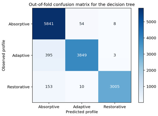
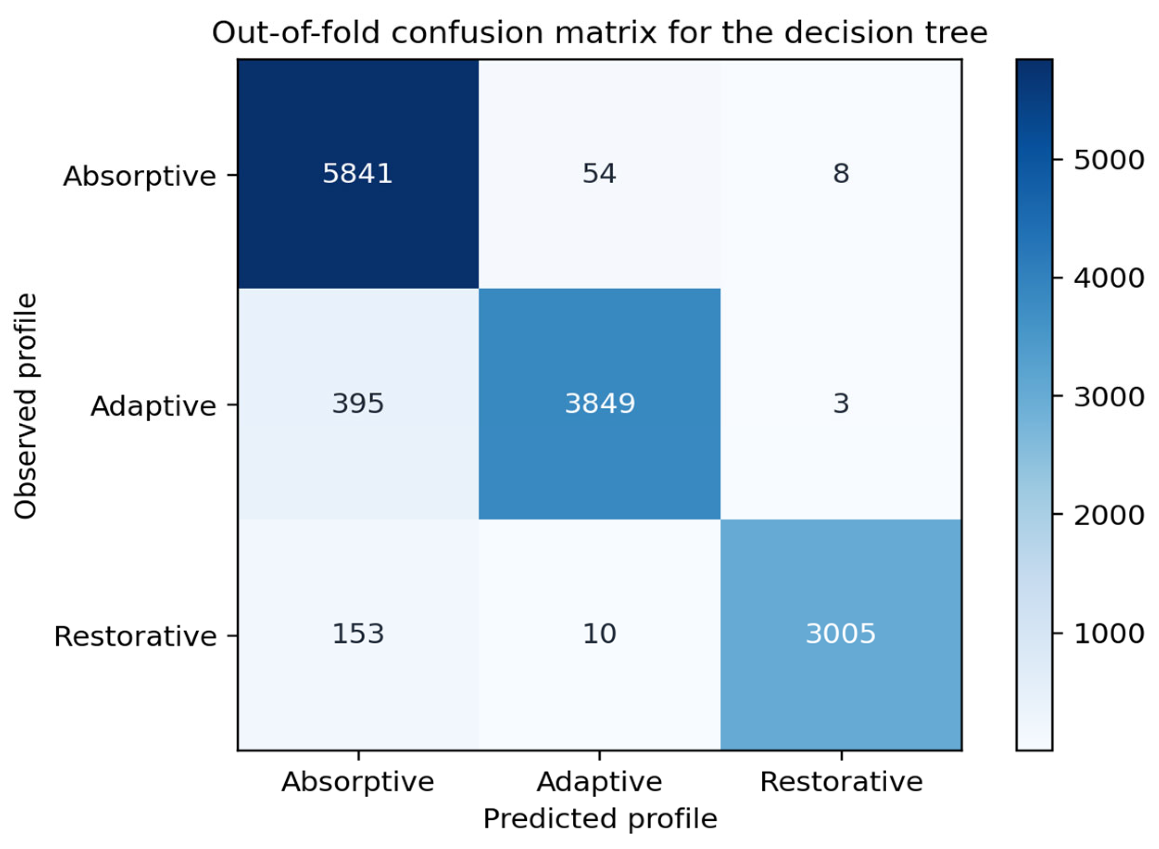
The adaptive class had the lowest recall (0.9063), versus 0.9895 for absorptive and 0.9485 for restorative observations. Predicted absorptive profiles accounted for many adaptive and restorative errors, motivating asymmetric audit-review sensitivity analysis.
Figure 1 shows the out-of-fold confusion matrix across supplier-disjoint outer tests.
Figure 1.
Out-of-fold confusion matrix for the depth-constrained decision tree.
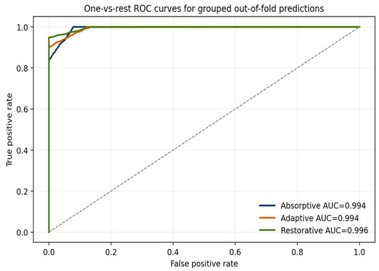
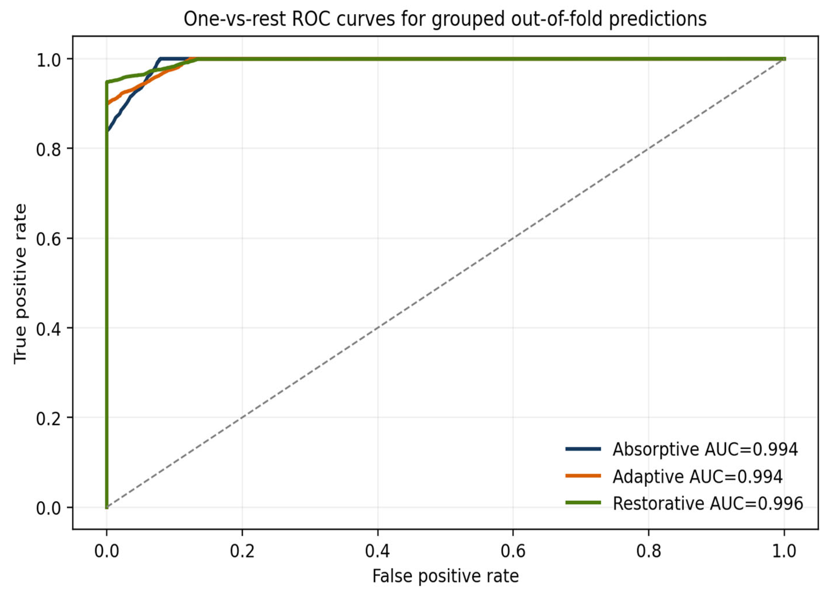
Figure 2 displays one-vs.-rest receiver operating characteristic (ROC) curves from grouped out-of-fold predictions.
Figure 2.
One-vs.-rest ROC curves based on grouped out-of-fold predictions.
4.3. Temporal Stability
Table 7 contains the chronological test in which all four models were fitted on January–September and evaluated on October–December 2025. The aggregate holdout values reported in Table 7 are also retained in Table S10 so that these results can be checked. The October–December test had 3334 records (1480 absorptive, 1053 adaptive and 801 restorative), and the preceding training period had 9984. The training period class supports were 4423 absorptive, 3194 adaptive and 2367 restorative records (total 9984), determined by subtracting the test period support from the full-year support. The holdout confusion matrix is given after Table 7.
Table 7.
Chronological holdout for October–December 2025.
For the supplementary, joint supplier-disjoint and time-ordered validation, the decision tree obtained accuracy 0.9496, macro-F1 0.9519, and balanced accuracy 0.9444; logistic regression obtained 0.7747/0.7666/0.7734, random forest 0.9484/0.9506/0.9438, and histogram gradient boosting 0.9493/0.9515/0.9468. This evaluation withholds supplier identities while preserving an earlier training window and later test window. Its scope remains confined to the 2025 study network and does not prove robustness to new external organizational settings.
For the records from the final quarter, the decision tree reached an accuracy of 0.9499 and a macro-F1 of 0.9522. Compared with the four-decimal mean values obtained from grouped cross-validation, accuracy was lower by about 0.0033 and macro-F1 by about 0.0030. These differences were small. In the observed final quarter, the model therefore showed little reduction in performance when evaluated using a test separate from the ten-fold partition. Table 8 presents the confusion matrix for the chronological holdout. Among 3334 test records, the model classified 3167 correctly, while 167 were classified incorrectly. In October, with 1089 records, accuracy was 0.9532 and macro-F1 was 0.9544. For November, the 1086 records gave an accuracy of 0.9521 and a macro-F1 of 0.9549. December included 1159 records, with accuracy of 0.9448 and macro-F1 of 0.9471. Although the model maintained relatively similar performance during these months, the results cannot exclude the possibility of population drift or concept drift.
Table 8.
Chronological holdout confusion matrix (rows, committee profiles; columns, predicted A = absorptive, D = adaptive, R = restorative).
4.4. Feature Importance and Depth Robustness
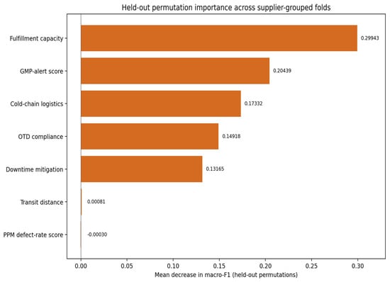
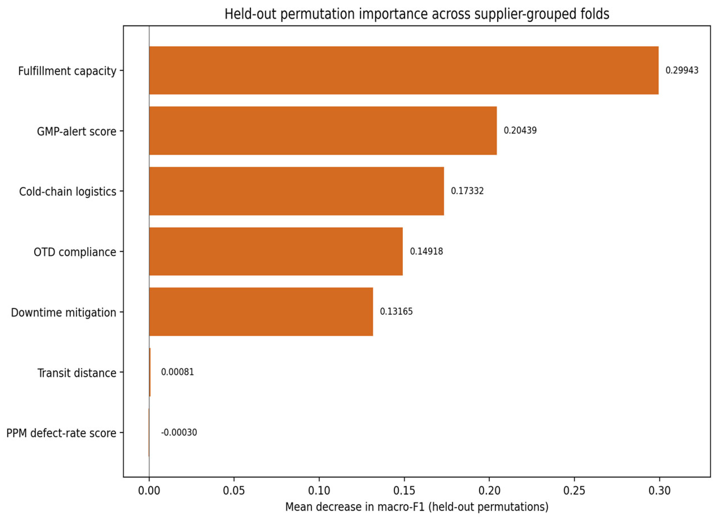
Figure 3 shows the permutation importance results obtained from the held-out data. In each test fold, the values of one predictor were permuted, and the resulting reduction in macro-F1 was measured. In this way, the importance of predictors was evaluated using observations that were not included in model fitting. The results therefore do not depend only on the impurity measures calculated within the decision tree.
Figure 3.
Out-of-fold permutation importance with five shuffles per predictor in each of ten supplier-disjoint outer folds; mean reduction in macro-F1.
Figure 3 ranks fulfillment capacity first (mean held-out macro-F1 loss 0.29943), followed by GMP-alert score (0.20439), cold-chain logistics (0.17332), OTD compliance (0.14918), and downtime mitigation (0.13165). Transit distance (0.00081) and PPM defect-rate score (−0.00030) had negligible incremental permutation effects. Each importance value reflects predictive association within the fitted procedure and has no causal interpretation; measures required for regulatory audits should not be discarded based only on a small importance estimate.
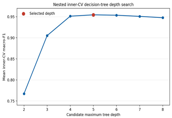
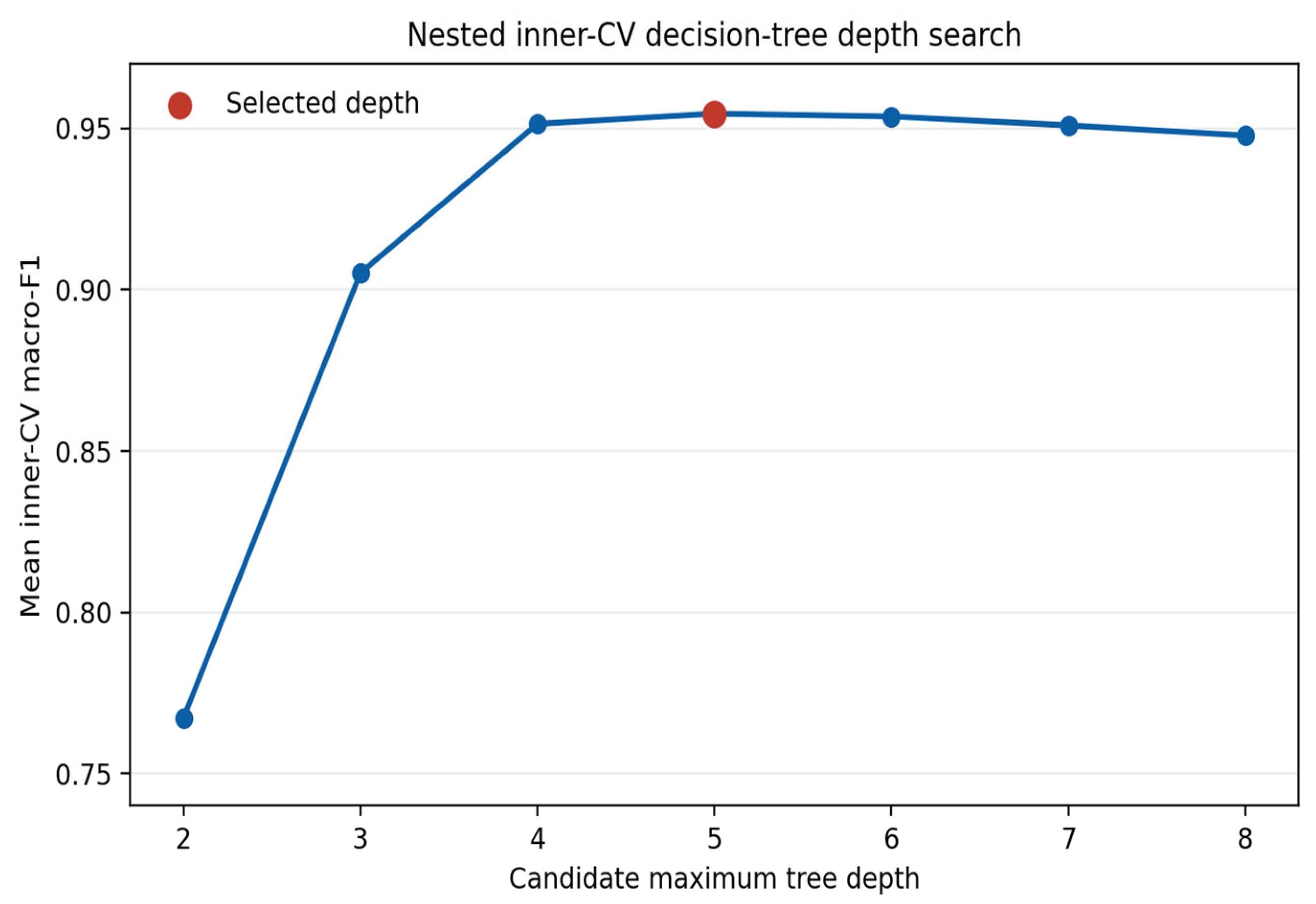
All 350 inner-validation evaluations are summarized in Figure 4. For depths two to eight, mean inner-CV macro-F1 was 0.7672, 0.9052, 0.9514, 0.9546, 0.9537, 0.9510, and 0.9478. Depth five has the largest mean. In the nested selections, it was chosen in seven outer folds; depth six was chosen in the other three.
Figure 4.
Mean inner-CV macro-F1 across the nested depth-search log (10 outer folds × 5 inner folds per candidate depth).
4.5. Unsupervised Diagnostics
Table 9 compares the primary K-means, hierarchical and DBSCAN diagnostics. The committee labels were assigned before clustering and were not used as cluster targets.
Table 9.
Selected clustering diagnostics (K-means, all 13,318 records; DBSCAN, label-stratified subsample of 4500 records).
In an independent subsample of 1800 records selected without using the labels, hierarchical clustering with complete linkage and Euclidean distance at k = 3 obtained an ARI of 0.0090 and an NMI of 0.0126. Using the range-normalized L1 distance metric, these values were 0.0526/0.0526 at k = 3 and 0.0749/0.0885 at k = 5. The DBSCAN results were also sensitive to the parameters and distance metric. In one Euclidean setting (η = 1.2), eight clusters were obtained, with approximately 84.6% of the data classified as noise. The normalized L1 metric produced three clusters with approximately 58.9% noise at η = 0.09 and one cluster with negligible noise at η = 0.17. Radius (η) values cannot be directly transferred between different distance metrics. Also, the subsample results should not be compared with the full-data statistics under the assumption that they represent the same population. These analyses only show the degree of separation produced by the examined geometric structures and do not invalidate the committee’s classification structure, nor do they indicate agreement with independently measured disruption outcomes.
5. Discussion
5.1. Interpretation of the Findings
Using supplier-grouped nested cross-validation, the decision tree reached a mean accuracy of 95.32% in reproducing committee-assigned profiles for suppliers not included in each training fold. The tree depth was selected separately within each outer-training partition. In the additional evaluation that considered both time and supplier separation, accuracy was also close to 95%. The main chronological holdout, however, tested later records of suppliers already known to the model. These results indicate that the recorded organizational labels can be reproduced with similar performance when supplier grouping and time are considered in the evaluation. However, they do not show that the model can independently predict actual shortages, losses caused by disruptions, or the time needed for recovery. In the grouped evaluation, the decision tree had an accuracy 18.8 percentage points higher than multinomial logistic regression. This difference suggests that nonlinear decision boundaries are important for reproducing the governance categories used in this study.
The predicted pattern was also consistent with the profile means. In the permutation analysis on the held-out data, fulfillment capacity was ranked first. It was followed by GMP alerts, cold-chain logistics, OTD compliance, and downtime mitigation. When these variables were considered together, distance and PPM provided little additional discriminatory power. However, this result is not causal. It also cannot be inferred from this result that a quality-control variable should be removed from supplier audits.
The validation challenge is not only leakage but also the meaning of the target; committee members accessed operational evidence overlapping with the seven predictors. Predicting their assignments may consequently recover implicit expert criteria. The high inter-rater agreement supports consistency among raters, not the absence of shared bias. The supervised and unsupervised results should therefore be read as complementary diagnostics about decision-rule reproducibility and geometric organization, rather than competing tests of a single independently measured resilience construct.
The difference between classification and clustering also clarifies what the model has learned. In the supervised analysis, a governance taxonomy was predicted that had previously been recorded by the committee based on the conditional combination of indicators. For K-means, hierarchical clustering, and DBSCAN to reproduce these categories, the committee-defined classes would also need to form clearly separated groups in the geometric structure of the data. The diagnostic results did not show such separation.
5.2. Managerial Use
The practical use of this model is mainly intended for periodic supplier review, not for automated purchasing decisions. After a new evaluation is recorded, the model proposes a profile together with a confidence value. However, this value does not represent a calibrated probability of operational risk. Cases with low confidence, or cases where the proposed profile differs from the committee’s assessment, are selected for further examination. Staff from procurement, quality, and logistics can review them. The decision tree uses a small number of thresholds, which makes it possible to follow the observations that resulted in a particular class being suggested. The original evaluation record is then checked to see whether the proposed classification agrees with the evidence recorded for that case.
The final tree prepared for explaining the classifications has 37 nodes and 19 leaves. Its maximum depth is five. The decision path from the root to every terminal leaf is stored, along with the predicted class and the support for that leaf. For practical use, each proposed profile would be recorded together with a snapshot of the input data and the version of the model. Procurement and quality staff would examine the result. If the evidence is conflicting, the case would be referred for further examination. After this review, the proposed profile would either be confirmed by a human reviewer or changed through an override, and this decision would be documented. Illustrative review thresholds based on the tree’s leaf scores are reported in Worksheet R17 of the Supplementary Materials; their use in practice still requires prospective validation.
Three examples from the fitted depth-five explanatory tree make the paths auditable. Absorptive leaf 35 (2971 training occurrences) requires fulfillment capacity > 3.5, OTD compliance > 2.5, and fulfillment capacity ≤ 4.5. Adaptive leaf 19 (2470 occurrences) requires fulfillment capacity ≤ 3.5, GMP-alert score > 2.5, cold-chain logistics > 2.5, and fulfillment capacity > 1.5. Restorative leaf 10 (1541 occurrences) requires fulfillment capacity ≤ 3.5, GMP-alert score ≤ 2.5 and downtime mitigation > 2.5. All 19 terminal rules, their supports and class-weighted leaf distributions are reported in Worksheet R15 of the Supplementary Materials. These paths describe fitted classifications, not documented historical committee decision rules.
The following are model-derived illustrative input examples, not disclosed audit records or reconstructed historical committee decisions. For an absorptive path, fulfillment = 4 and OTD = 3 satisfy the reported leaf-35 conditions; the proposed audit emphasis is immediate fulfillment and delivery continuity. For an adaptive path, fulfillment = 3, GMP-alert score = 3 and cold-chain score = 3 satisfy the reported leaf-19 conditions; the reviewer would examine documented cold-chain alternatives and compliance response. For a restorative path, fulfillment = 3, GMP-alert score = 2 and downtime mitigation = 3 satisfy the reported leaf-10 conditions; attention would turn to recovery plans and downtime escalation. Other predictors remain subject to audit and are not asserted to be immaterial for a real supplier. These examples illustrate the reported threshold logic only, and provide no independent evidence that the corresponding profiles predict realized disruptions.
Table 10 summarizes the profile-specific priorities for human audit review.
Table 10.
Governance priorities suggested by each resilience profile.
The activities shown in Table 10 relate to the goal of the review and are not order-allocation decisions. Order quantities depend on variables such as the level of demand, production capabilities, acquisition and transportation costs, minimum order quantities, lead time, importance of the items and possible disruption scenarios. Although profile probabilities could later be introduced as risk or eligibility criteria, this would involve a separate optimization model.
The last-quarter confusion matrix contained 167 incorrect assignments, of which 149 were committee-adaptive or committee-restorative occurrences predicted as absorptive. Classification errors may not have the same consequences. To examine this, a hypothetical cost matrix was considered. When one unit of cost is assigned to every error, the total for 167 errors is 167 units. If the 149 specified errors are instead given a cost five times higher, the total reaches 763 units. With ten times the cost for those errors, the total is 1508 units. These figures are dimensionless and are used only to illustrate possible scenarios. They are not financial losses measured from actual disruptions. The choice of a model policy or review procedure may change if other ratios of error costs are considered. Also, the scores given at the leaves of the decision tree do not represent calibrated probabilities of operational risk. This is particularly important when class weighting has been applied. Before operational thresholds are introduced, or an automated review policy is used, the scores would need to be calibrated. The assumed costs must also have justification from external evidence, and the policy would need prospective approval through the governance process.
Some controls are also necessary if the model is used after implementation. Whenever the model is trained again, the records should continue to be grouped by supplier. Changes in the share of each class and the performance of the model in later periods also need to be monitored by the organization. Experts may sometimes change the classification proposed by the model. In such cases, the reason for the change should be documented. These records can help determine whether the thresholds used by the model remain appropriate. Related systems research also considers risk control, resource allocation, and human responsibility in the design of decision-support systems [24].
5.3. Implications for Resilient Operations and Information Governance
Supplier auditing requires the exchange of operational information and quality-related evidence among purchasing, logistics, and quality assurance departments. Studies on supply chain integration show that information coordination is related to operational flexibility and resilience [25]. The contribution of this study is to provide a traceable process from data recording to the application of model rules and the review of results. In this process, supplier identifiers are retained for the evaluation design, the source of each score is recorded, and the final decision about the profiles remains the responsibility of the experts.
6. Research Boundaries and Future Work
The study evaluates committee-assigned profiles within one pharmaceutical distribution network in 2025, not independently observed shortages, disruption losses or recovery durations. The committee members had access to evidence that overlapped with the seven predictors. Therefore, even a high level of agreement among the raters does not confirm construct validity. The model may also reproduce part of the assessment criteria shared by the committee when it predicts the recorded labels. The collaborating data provider confirmed the direction of the ordinal scales, profile concepts and adjudication procedure; however, complete historical coding manuals and individual files for the 17 tied cases were not independently audited. Furthermore, multiple occurrences under the same supplier–hub–month key cannot be attributed to distinct inspections or amendments without event, shipment, product or batch identifiers.
The primary chronological holdout contained all 441 suppliers in both the training and test periods, so it represents future evaluations of known suppliers. The complementary time-aware supplier-disjoint experiment assesses withheld suppliers within this network, but does not constitute an external prospective cohort. One-per-key refits were stable without establishing the operational independence of repeated occurrences. The Euclidean and label-stratified clustering diagnostics were supplemented with range-normalized L1 and label-independent analyses; these remain sensitive to distance assumptions and do not establish or refute an independently validated resilience taxonomy.
A prospective study could test whether profile probabilities are related to shortage duration, service continuity, recovery time, or disruption loss. Product and batch identifiers would also permit analysis at the supplier–hub–product–time level. Before using probabilities for automatic review rules, their calibration and the cost of different classification errors should be examined. A later allocation model could then combine the validated probabilities with demand, capacity, cost, service, and regulatory restrictions.
7. Conclusions
The analysis was based on 13,318 confidential recorded evaluations belonging to 441 suppliers. The main question was whether a machine learning classifier, whose decisions can be traced, could reproduce the three supplier profiles already defined by the committee. For the decision tree, nested ten-fold validation was applied, keeping suppliers in the training and test groups separate. The depth of the tree was chosen within each outer training partition, without using the corresponding test data. Mean accuracy was 0.9532, while macro-F1 reached 0.9552. The supplier-cluster bootstrap intervals, calculated from fixed held-out predictions, were approximately 0.9499–0.9566 for accuracy and 0.9520–0.9585 for macro-F1. A separate evaluation on the final quarter gave an accuracy of 0.9499. In that evaluation, however, the suppliers were already present during training, so the test did not include previously unseen suppliers. When both time and supplier separation were considered, accuracy was 0.9496 within the same pharmaceutical distribution network. This evaluation does not constitute external validation or establish generalizability to other organizations. The results remained comparable to the complete-data analysis when the models were refitted with only one occurrence for each key. Histogram gradient boosting gave performance close to the decision tree. The tree, however, had decision paths that could be followed and examined directly.
According to the held-out permutation diagnostics, the most important contributions to reproducing the recorded committee profiles came from fulfillment, GMP-alert-associated scores, cold-chain logistics, delivery compliance, and downtime mitigation. A different result was obtained from unsupervised clustering. K-means, hierarchical clustering, and DBSCAN showed low agreement with the profiles assigned by the committee. The amount of agreement was also affected by the distance definition and sampling procedure. This low agreement does not, by itself, show that the committee’s categories are invalid. What the findings support is the use of a traceable classification model to help reproduce organizational audit profiles, while human reviewers remain responsible for the decisions. The results cannot be taken as an independent measure of actual supplier resilience, or as evidence about the causal factors behind it. They also do not support using the model for automatic order allocation. Stronger conclusions about predictive ability or operational application would require prospective observations of actual disruptions, verification of the full governance documentation, and validation of asymmetric decision costs.
Supplementary Materials
The following supporting information can be downloaded at: https://www.mdpi.com/article/10.3390/systems14111408/s1. A non-confidential workbook is provided with this study. It includes definitions of the variables, results of supplier-grouped validation, clustering diagnostics, permutation importance, and the chronological and time-aware supplier-disjoint evaluations. The workbook also contains uncertainty intervals, model comparison tests, and the complete rules extracted from the decision tree. The main supplementary tables are numbered S2–S10, while the additional sheets for sensitivity analyses are numbered R0–R19. Both groups are listed in the workbook index. The restricted operational records and individual ratings are not included in the publicly available supplement.
Funding
This research received no external funding.
Institutional Review Board Statement
Not applicable. Anonymized records of business operations were the only data used in this research. The study did not involve human participants. Patient data and personal data were not used either.
Informed Consent Statement
Not applicable.
Data Availability Statement
Definitions of the variables and the results of analyses at aggregate level are provided in the non-confidential Supplementary Workbook. The operational data for individual records remain confidential and are not publicly available. Public access is also not provided to the anonymized supplier identifiers or the assessments of individual committee members. The corresponding author may consider requests for further information. Before any information can be shared, specific authorization must be obtained from the collaborating data provider. The applicable confidentiality requirements also need to be met. Access to additional information, therefore, is not guaranteed.
Acknowledgments
The author thanks the collaborating pharmaceutical network for sharing de-identified operational records. Non-confidential explanations about the procedures used for coding and auditing were also provided by the network. During the preparation of this manuscript, the author used Ginger Software (version 2.8.73) and Grammarly (version 1.2.305.1980) for grammar checking, language refinement, readability improvement, and formatting consistency. The author has reviewed and edited the output and takes full responsibility for the content of this publication.
Conflicts of Interest
The author declares no conflicts of interest.
References
- Adobor, H.; McMullen, R.S. Supply chain resilience: A dynamic and multidimensional approach. Int. J. Logist. Manag. 2018, 29, 1451–1471. [Google Scholar] [CrossRef] [Scilit]
- Ribeiro, J.P.; Barbosa-Póvoa, A. Supply chain resilience: Definitions and quantitative modelling approaches—A literature review. Comput. Ind. Eng. 2018, 115, 109–122. [Google Scholar] [CrossRef] [Scilit]
- Ivanov, D.; Dolgui, A. Viability of intertwined supply networks: Extending the supply chain resilience angles towards survivability. Int. J. Prod. Res. 2020, 58, 2904–2915. [Google Scholar] [CrossRef] [Scilit]
- Hosseini, S.; Al Khaled, A. A hybrid ensemble and AHP approach for resilient supplier selection. J. Intell. Manuf. 2019, 30, 207–228. [Google Scholar] [CrossRef] [Scilit]
- Hosseini, S.; Tajik, N.; Ivanov, D.; Sarder, M.D.; Barker, K.; Al Khaled, A. Resilient supplier selection and optimal order allocation under disruption risks. Int. J. Prod. Econ. 2019, 213, 124–137. [Google Scholar] [CrossRef] [Scilit]
- Urmston, A.; Song, D.; Lyons, A. The development of risk assessments and supplier resilience models for military industrial supply chains considering rare disruptions. Logistics 2024, 8, 57. [Google Scholar] [CrossRef] [Scilit]
- Baryannis, G.; Dani, S.; Antoniou, G. Predicting supply chain risks using machine learning: The trade-off between performance and interpretability. Future Gener. Comput. Syst. 2019, 101, 993–1004. [Google Scholar] [CrossRef] [Scilit]
- Tirkolaee, E.B.; Sadeghi, S.; Mooseloo, F.M.; Vandchali, H.R.; Aeini, S. Application of machine learning in supply chain management: A comprehensive overview of the main areas. Math. Probl. Eng. 2021, 2021, 1476043. [Google Scholar] [CrossRef] [Scilit]
- Cavalcante, I.M.; Frazzon, E.M.; Forcellini, F.A.; Ivanov, D. A supervised machine learning approach to data-driven simulation of resilient supplier selection in digital manufacturing. Int. J. Inf. Manag. 2019, 49, 86–97. [Google Scholar] [CrossRef] [Scilit]
- Ali, M.R.; Nipu, S.M.A.; Khan, S.A. A decision support system for classifying supplier selection criteria using machine learning and random forest approach. Decis. Anal. J. 2023, 7, 100238. [Google Scholar] [CrossRef] [Scilit]
- Kang, P.S.; Bhawna, B. Enhancing supply chain resilience through supervised machine learning: Supplier performance analysis and risk profiling for a multi-class classification problem. Bus. Process Manag. J. 2025, 31, 2825–2848. [Google Scholar] [CrossRef] [Scilit]
- Li, X.; Krivtsov, V.; Pan, C.; Nassehi, A.; Gao, R.X.; Ivanov, D. End-to-end supply chain resilience management using deep learning, survival analysis, and explainable artificial intelligence. Int. J. Prod. Res. 2025, 63, 1174–1202. [Google Scholar] [CrossRef] [Scilit]
- Gidiagba, J.O.; Tartibu, L.K.; Okwu, M.O. A systematic review of machine learning applications in sustainable supplier selection. Decis. Anal. J. 2025, 14, 100547. [Google Scholar] [CrossRef] [Scilit]
- Kapoor, S.; Narayanan, A. Leakage and the reproducibility crisis in machine-learning-based science. Patterns 2023, 4, 100804. [Google Scholar] [CrossRef] [Scilit]
- Roberts, D.R.; Bahn, V.; Ciuti, S.; Boyce, M.S.; Elith, J.; Guillera-Arroita, G.; Hauenstein, S.; Lahoz-Monfort, J.J.; Schröder, B.; Thuiller, W.; et al. Cross-validation strategies for data with temporal, spatial, hierarchical, or phylogenetic structure. Ecography 2017, 40, 913–929. [Google Scholar] [CrossRef] [Scilit]
- Varma, S.; Simon, R. Bias in error estimation when using cross-validation for model selection. BMC Bioinform. 2006, 7, 91. [Google Scholar] [CrossRef] [Scilit]
- Rudin, C. Stop explaining black box machine learning models for high stakes decisions and use interpretable models instead. Nat. Mach. Intell. 2019, 1, 206–215. [Google Scholar] [CrossRef] [Scilit]
- Almadani, B.; Kaisar, H.; Thoker, I.R.; Aliyu, F. A systematic survey of distributed decision support systems in healthcare. Systems 2025, 13, 157. [Google Scholar] [CrossRef] [Scilit]
- Papalexi, M.; Vafadarnikjoo, A.; Bamford, D.; Dehe, B. Developing pharmaceutical supply chain resilient capabilities: The role of Industry 4.0 technologies. Supply Chain Manag. Int. J. 2026, 31, 1–20. [Google Scholar] [CrossRef] [Scilit]
- Esmaeili, M.; Olfat, L.; Amiri, M.; Raeesi Vanani, I. Classification and allocation of suppliers to customers in resilient supply chains using machine learning. Ind. Manag. Perspect. 2023, 13, 39–70. [Google Scholar] [CrossRef]
- Pedregosa, F.; Varoquaux, G.; Gramfort, A.; Michel, V.; Thirion, B.; Grisel, O.; Blondel, M.; Prettenhofer, P.; Weiss, R.; Dubourg, V.; et al. Scikit-learn: Machine learning in Python. J. Mach. Learn. Res. 2011, 12, 2825–2830. [Google Scholar]
- Breiman, L. Random forests. Mach. Learn. 2001, 45, 5–32. [Google Scholar] [CrossRef] [Scilit]
- Friedman, J.H. Greedy function approximation: A gradient boosting machine. Ann. Stat. 2001, 29, 1189–1232. [Google Scholar] [CrossRef] [Scilit]
- Almalki, S.S. AI-driven decision support systems in agile software project management: Enhancing risk mitigation and resource allocation. Systems 2025, 13, 208. [Google Scholar] [CrossRef] [Scilit]
- Siagian, H.; Tarigan, Z.J.H.; Jie, F. Supply chain integration enables resilience, flexibility, and innovation to improve business performance in COVID-19 era. Sustainability 2021, 13, 4669. [Google Scholar] [CrossRef] [Scilit]

Disclaimer/Publisher’s Note: The statements, opinions and data contained in all publications are solely those of the individual author(s) and contributor(s) and not of MDPI and/or the editor(s). MDPI and/or the editor(s) disclaim responsibility for any injury to people or property resulting from any ideas, methods, instructions or products referred to in the content. |
© 2026 by the author. Licensee MDPI, Basel, Switzerland. This article is an open access article distributed under the terms and conditions of the Creative Commons Attribution (CC BY) license.