Analysis and Comparison of Bitcoin and S and P 500 Market Features Using HMMs and HSMMs †


Faculty of Science, University of Malta, Msida 2080, Malta
*
Author to whom correspondence should be addressed.
†
This is the extended version of our previous conference paper presented in the 2nd International Workshop on Blockchain and Smart Contract Technologies (BSCT 2019) which is in conjunction with the 22nd International Conference on Business Information Systems, 26–28 June 2019.
‡
These authors contributed equally to this work.
Information 2019, 10(10), 322; https://doi.org/10.3390/info10100322
Submission received: 28 September 2019
/
Revised: 11 October 2019
/
Accepted: 16 October 2019
/
Published: 18 October 2019
(This article belongs to the Special Issue Blockchain and Smart Contract Technologies)
Abstract
:We implement hidden Markov models (HMMs) and hidden semi-Markov models (HSMMs) on Bitcoin/US dollar (BTC/USD) with the aim of market phase detection. We make analogous comparisons to Standard and Poor’s 500 (S and P 500), a benchmark traditional stock index and a protagonist of several studies in finance. Popular labels given to market phases are “bull”, “bear”, “correction”, and “rally”. In the first part, we fit HMMs and HSMMs and look at the evolution of hidden state parameters and state persistence parameters over time to ensure that states are correctly classified in terms of market phase labels. We conclude that our modelling approaches yield positive results in both BTC/USD and the S and P 500, and both are best modelled via four-state HSMMs. However, the two assets show different regime volatility and persistence patterns—BTC/USD has volatile bull and bear states and generally weak state persistence, while the S and P 500 shows lower volatility on the bull states and stronger state persistence. In the second part, we put our models to the test of detecting different market phases by devising investment strategies that aim to be more profitable on unseen data in comparison to a buy-and-hold approach. In both cases, for select investment strategies, four-state HSMMs are also the most profitable and significantly outperform the buy-and-hold strategy.
1. Introduction
This article extends the results given in the conference paper in [1], where we present the best-fitting hidden semi-Markov model (HSMM) model (four-state in both cases) for both Bitcoin/US dollar (BTC/USD) and Standard and Poor’s 500 (S and P 500) from a number of hidden Markov models (HMMs) and HSMMs considered. In the latter, we also interpret the different states for both series in terms of market phases, and we introduce a number of investment strategies, some of which we find to be significantly profitable when using four-state HSMMs. In addition to the conference paper, this article presents the following new findings and further material: (i) optimal HMM model outputs for BTC/USD and S and P 500 series are also presented; (ii) more detailed statistical properties of the models are given in terms of bootstrap confidence intervals for optimal HMMs and HSMMs of both series; (iii) the evolution of state and persistence parameters across time in the test set for both HMMs and HSMMs is looked into for both BTC/USD and S and P500, motivating further the decision of how HSMM states are labelled in terms of market phases; (iv) an additional strategy (Strategy 4) is proposed in Section 4 related to investment strategies, and its performance is also assessed; (v) for all strategies, results for all grid points considered in Strategies 3 and 4 are presented (whereas in [1], only Strategy 3 was presented, and only for optimal ); (vi) plots are presented showing when buy and sell actions were suggested by our optimal model/strategy combination for both BTC/USD and the S and P 500 (in [1], only return on investment (ROI) at the end of the testing period is shown, whereas these figures demonstrate both instances when buy/sell strategies led to profit and instances that led to loss).
We start by giving a brief background on cryptocurrencies. Following the publishing of the Bitcoin white paper by Satoshi Nakamoto (see [2]) in November 2008, the first Bitcoin transaction was made in January 2009, with other cryptocurrencies following in subsequent years. Since then, a number of key events led to an increase in their importance; however, cryptocurrencies mostly received hype and widespread public recognition in 2017. The history of Bitcoin and other cryptocurrencies is filled with numerous events that have drastically affected their value, and scholarly literature, official reports, and media in general, are full of discussion regarding their price dynamics and volatility. The following are some of the most given reasons for why intense volatility is experienced by cryptocurrencies: (i) cryptocurrency investor bases are smaller than traditional stock markets with large holders and these can severely sway the markets through their actions (see, e.g., [3]); (ii) due to considerably polarised views about cryptocurrencies in the general public, media and social media can greatly affect their value (see, e.g., [4,5,6]); and (iii) cryptocurrencies are highly subject to speculation (see, e.g., [3,4,6,7,8]). In recent history, while 2017 was generally a bull year for cryptocurrencies, 2018 saw great decline in their value, and some cryptocurrencies have been wiped out. Currently, however, the value of one Bitcoin has more than doubled its price since its 2019 low. Meanwhile, while cryptocurrencies are unregulated by central banking systems, regulatory action (both for and against) by many jurisdictions has been taken.
The aim of this paper is that of identifying market regime patterns of cryptocurrencies through the use of HMMs and HSMMs, where we assume that each state follows a Gaussian distribution with both parameters dependent on the states. Furthermore, we look into the evolution of the parameters of each distribution across time on a chosen test set. To test our models, we implement mock investment strategies on test data and compare this to a buy-and-hold approach to determine how well these regimes are identified. It is customary to say that when prices are on the rise for a relatively long period of time, the market condition is a bull market, and when prices fall steeply with respect to recent highs, the market condition is a bear market. Two other phases that may be found in the process are corrections and rallies, with the former being a period of steady decrease amid a bull market and the latter being a period of slow increase within a bull or bear market. It is possible that HMMs and HSMMs may struggle to distinguish between these two states due to the fact that neither is associated with a steep change. Due to a high correlation between movements of various cryptocurrencies, we focus on the daily closing prices of BTC/USD, the most mature cryptocurrency, for the dates ranging from 1 January 2016 to 28 January 2019, for a total of 1124 trading days. Bitcoin is around 50% of the cryptocurrency market. Since traditionally, positive trends with low volatility and negative trends with high volatility have respectively been labelled as bull and bear markets, we compare and contrast our findings with a de facto standard stock market—the S and P 500, where the dates considered are 1 January 2000–28 January 2019. This can be invested in collectively via the S and P 500 Index Fund.
The following is a review of existing literature related to cryptocurrencies and the use of HMMs and HSMMs to model financial assets. Starting with the former, Reference [9] fit various parametric distributions on cryptocurrency returns. Furthermore [10,11,12,13,14] fit GARCH models and its variants in their single-regime form. Reference [15] looks at the application of Markov switching autoregressive models to Bitcoin. Recent publications that involve the modelling of Bitcoin volatility dynamics at multiple regimes are [16,17]—though different approaches were used for modelling in these papers with slightly varying results, in all cases, multiregime dynamics within a heteroscedastic framework were detected. Other literature in a different direction includes Reference [18], which proposes a time-varying parameter VAR model that incorporates Bayesian shrinkage priors for the purpose of introducing regularisation in the model framework, and Reference [19], which performs a Bayesian change-point analysis of Bitcoin. The following, on the other hand, are examples of literature using HMMs and HSMMs to model different phases of financial asset price movements. Reference [20] shows that a normal HMM is capable of reproducing most of the stylised facts for daily S and P 500 return series established by [21]. However, they only allow the standard deviations to vary by the state, while the means are fixed at zero. Recently, Reference [22] applied a four-state HMM for stock trading by predicting monthly closing prices of the S and P 500, showing that the HMM is superior to the buy-and-hold strategy as it yields larger percentage profits under different training and testing periods. Modelling literature on financial time series using HSMMs is, however, quite limited. Reference [23] compared HMMs and HSMMs when modelling the daily returns of 18 pan-European industry portfolios. They concluded that the HSMM with a negative binomial dwell-time distribution is a better alternative than the geometric distribution for HMMs. Reference [24] implemented a three-state HSMM to describe the dynamics of the Chinese Stock Index 300 (CSI 300) returns. The authors assumed normal state-dependent distributions with logarithmic dwell-time distributions and also implemented a profitable trading strategy.
In this paper, what we aim to do over and above the cited literature is to assess how the HMM and HSMM methodology for market phase detection performs within the cryptocurrency context by looking at BTC/USD and also drawing comparisons with benchmark stock such as the S and P 500. Furthermore, apart from implementation on Chinese stock in [24], the implementation of HSMM methodology on the S and P 500 or other traditional stocks has not been encountered in other literature we have reviewed. In the next section, we discuss the modelling approach implemented in this paper.
2. General Methodology
The daily adjusted close prices of BTC/USD and the S and P 500 were obtained for suitably chosen time periods, not equal in length, that encapsulate the swings the financial instrument goes through. Log returns of the daily adjusted close prices were taken, and the HMM and HSMM models were then fitted on the log returns. Mathematically, an m-state HMM consists of two processes: (i) an unobserved (hidden) discrete-time m-state Markov chain, , taking values in a finite state-space, , and (ii) a state-dependent process, , whose outcomes (observations) are assumed to be generated by one of m distributions corresponding to the current state of the underlying discrete-time Markov chain (DTMC). The distribution of is assumed to be conditionally independent of previous observations and states, given the current state . Such dynamics can be represented by the probabilities and the mass/density function the latter depending on the nature of the observations. For stationary HMMs, we denote by the resulting stationary probabilities of the underlying DTMC. For a thorough review of HMMs, refer to [25].
One drawback of basic HMMs is due to the one time lag memory of the underlying first order DTMC, which is inherently geometric. This means that the probability mass function of the dwell-time (i.e., the time spent) in state i, denoted by , is given by . One possible way to circumvent this problem is to consider general state (not necessarily geometric) dwell-time distributions, leading to the HSMM framework. Thus, HSMMs generalise HMMs by explicitly modelling state persistence and state switches separately. This is achieved by considering a DTSMC, with state-space . The state-dependent process for HSMMs is defined in the same way as the HMM case. Thus, the only difference between HMMs and HSMMs lies in the hidden state process. In this case, we define and let be any discrete non-negative probability mass function. Finally, we denote by the initial probabilities of the DTSMC. For a thorough account of HSMMs, refer to [23] and references therein. Since the log returns take values in the real space , we assume the state-dependent process to be distributed as normal with mean and standard deviation , where the s and s are the means and standard deviations for each state, for both HMMs and HSMMs. Moreover, the HSMM specification assumes that is distributed as a negative binomial with parameters , where the s and s are the negative binomial parameters for each state.
Parameter estimation of HMMs can be carried out by either direct numerical maximisation (DNM) of the likelihood via Newton-type methods or by the expectation maximisation (EM) algorithm. Both methods are described in [25]. HSMMs are usually fitted via the EM algorithm as described in [26]. For HMMs, the parameters we estimate are the s, the s, and the s, while the s are a direct consequence of the transition probabilities (refer to Tables 2 and 5). For HSMMs, the parameters we estimate are the ’s, the s, the s, the s, the s, and the s (refer to Tables 3 and 6). For HMMs, the Viterbi algorithm in [27] can be applied for both HMMs and HSMMs to obtain a sequence of most likely hidden states. In other words, the aim of the Viterbi algorithm is to seek the particular sequence of states that maximise the conditional probability , where N is the length of the series considered and represents the state at time n. Hence, by labelling the order of the states according to the Viterbi algorithm, one deciphers the most probable market phases based on the entire observable sequence of log returns, which in turn guide us in making profitable investments. Such a procedure is called global decoding.
The daily log return series are hence analysed as follows: (i) suitable HMMs and HSMMs on the complete time series are fitted by varying the number of assumed states; (ii) the optimal model based on the Akaike information criterion (AIC), Bayesian information criterion (BIC), and Hannan–Quinn criterion (HQC) is chosen; (iii) the chosen time period is split into mutually exclusive training and testing periods; (iv) an expanding window method is implemented by first fitting the optimal model on the training set and then iteratively adding one time-point from the test set (until the testing period is exhausted) to the training period and applying the Viterbi algorithm as a filtering procedure to nowcast the current most likely hidden state after parameter re-estimation; (v) the evolution of the mean and variance parameters of each state across time are analysed on the chosen test set; and (vi) finally, investment strategies based on the model features arising from the Viterbi algorithm are applied to determine models’ success at determining market phases. The data analysis presented next was carried out using R packages HiddenMarkov from [28] and hsmm from [29].
3. Model Results
In this section, we look at the modelling of the different market phases—first of BTC/USD, and then followed by S and P 500 for eventual comparison.
3.1. Bitcoin/USD Exchange Rate
HMMs and HSMMs were applied to the daily closing prices of the BTC/USD exchange rate. Figure 1 provides the sequence plots of BTC/USD (adjusted) close prices, , and the daily log returns, . As can be observed, up to 2017 the close prices exhibit steady but small rises, while between 2017 and 2018 the close prices rise very aggressively, with a sharp decline at the end. From 2018 onwards, there seems to be a negative overall trend with few ups and downs in between. The daily BTC/USD log returns seem to be characterised by volatility clustering, i.e., the tendency for low (or high) volatilities to occur in clusters. Summary statistics of reveal that the mean and variance are equal to 0.1854 and 16.6094, respectively. The coefficient of skewness is negative (−0.2077), implying that the distribution of log returns is left-tailed. Another stylised fact that is characterised by the series is that the coefficient of kurtosis greatly exceeds three (7.0052), implying a highly leptokurtic distribution. Non-normality of the series is supported by the Jarque–Bera test (statistic: 759.36, p-value: 0.00), which rejects the null hypothesis that the series follows a normal distribution at a 0.01 level of significance.
Table 1 summarises the model-fitting results on the complete series via the negative log-likelihood , AIC, BIC, and HQC for HMMs (where the underlying discrete-time Markov chains were assumed to be stationary) and HSMMs with different numbers of states. Note that the means and variances of the resulting mixtures of the two-, three-, and four-state HMMs were computed. As can be observed, the resulting means and variances are close to the sample statistics, which suggests that the regime-switching models fit the data well. We see that, according to the information criteria considered, the four-state models provide the best fit to the complete data. Note that, with regards to the normal HMMs, the BIC suggests that three states provides the best fit.
The parameter estimates and 90% confidence intervals (based on the parametric bootstrap method) for the stationary four-state normal HMM are summarised in Table 2. As a general rule, we shall now refer to estimates of parameters with a over the symbol. From the stationary probabilities, , it is evident that the four-state normal HMM spends most of its time in state 3 (35.7%), which is characterised by a positive mean and moderately high volatility. The least time is spent in state 4 (17.1%), which is the only state characterised by a negative mean and the highest volatility. Of particular interest are the transition probability estimates, , which show a lack of strong persistence in states 1 and 2. Consequently, we interpret the model as follows. State 3 can be associated with a bull market due to the moderately high mean and strong persistence. State 4 can be associated with a bear market due to the large (and only) negative mean with relatively weak persistence. Both states exhibit very high volatility, though the bear state exhibits a stronger drift and volatility. Attaching interpretations to state 1 and 2 can be a bit more tricky, as both have weak persistence. State 1 appears to be a market correction/rally state due to its low drift and volatility, while state 2 appears to be an additional bull state with stronger drift, smaller volatility, and weak persistence.
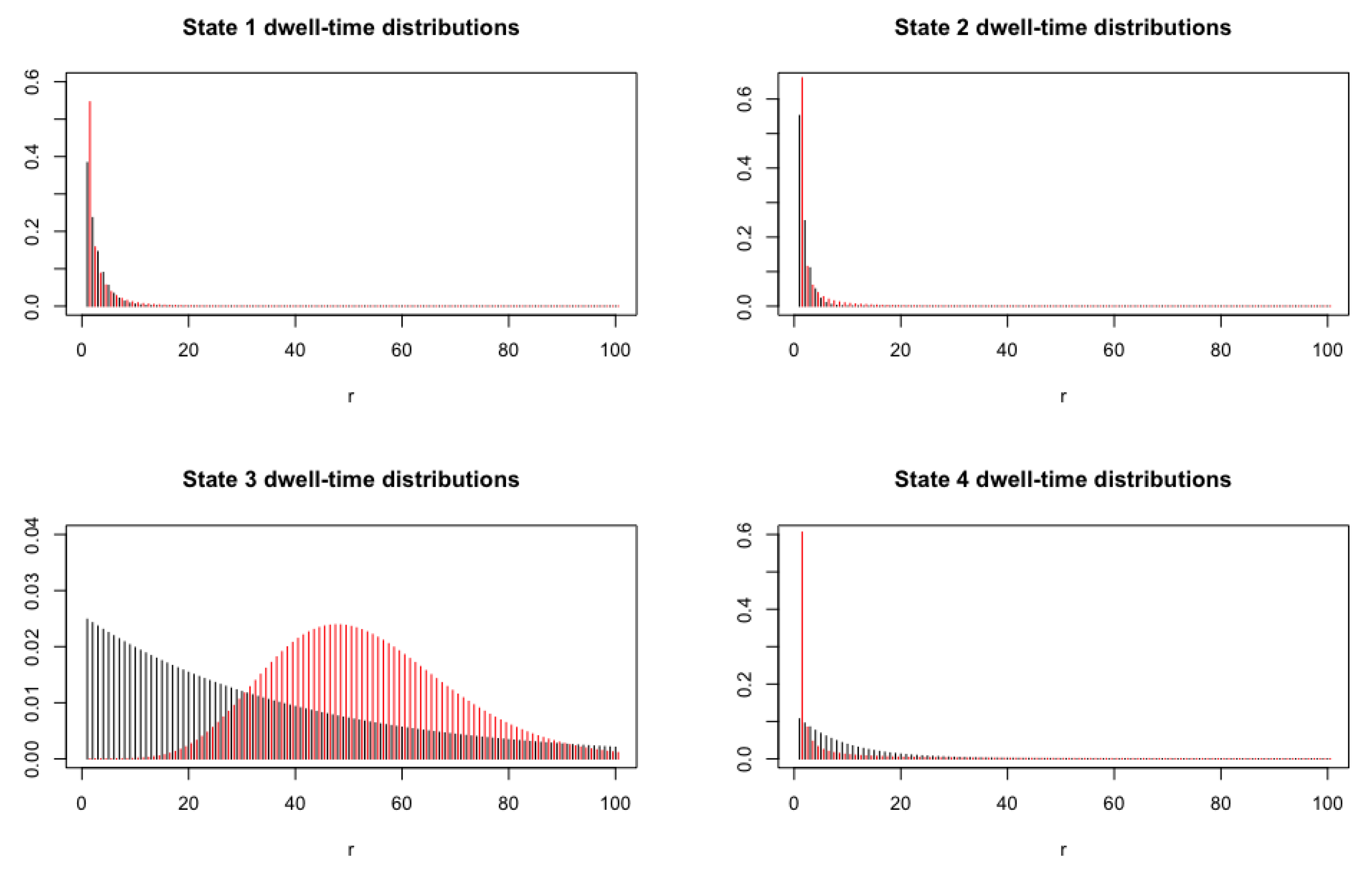
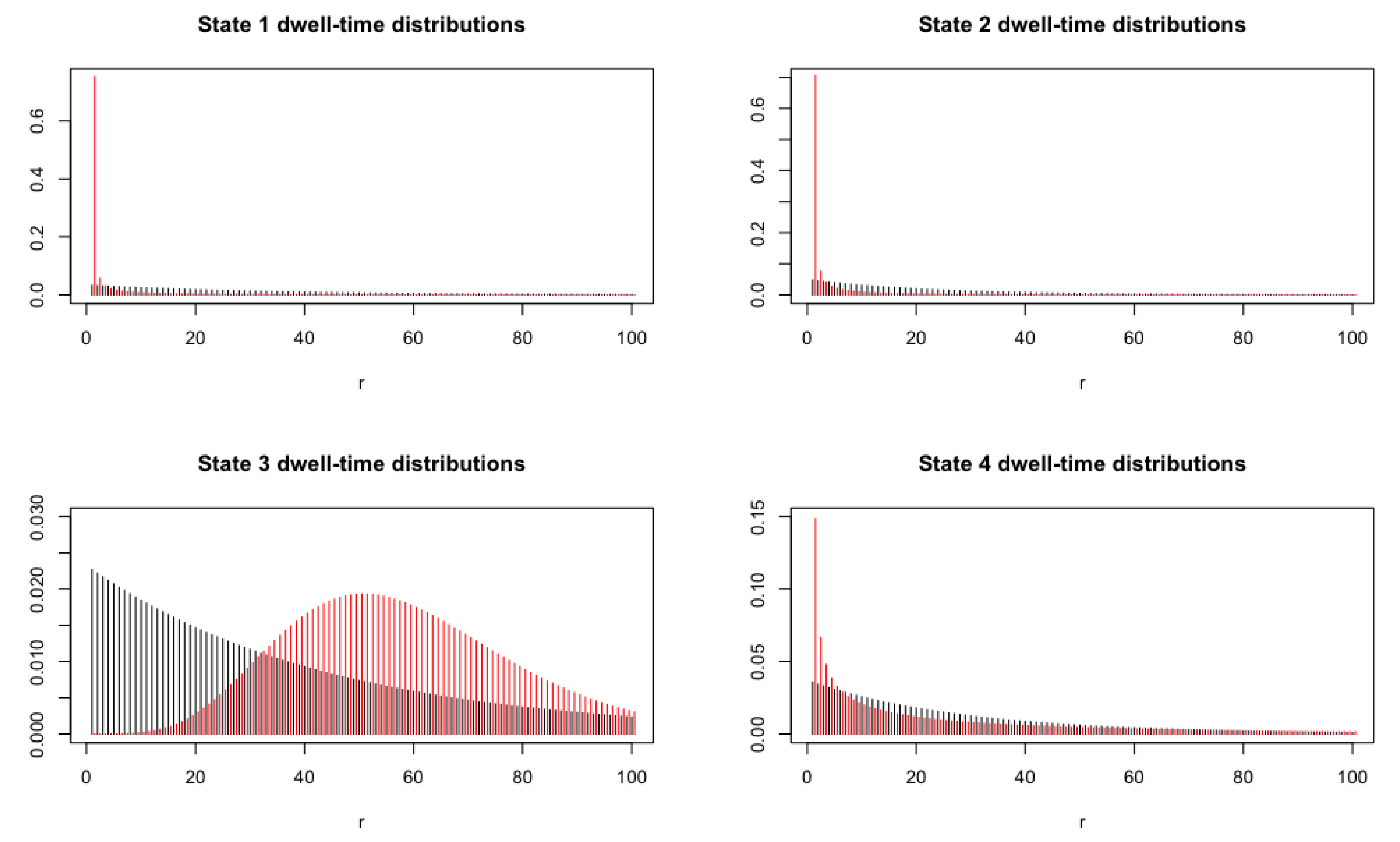
The parameter estimates and 90% confidence intervals (based on the parametric bootstrap method) for for the homogeneous four-state normal HSMM, fitted via the EM algorithm, are presented in Table 3. The initial distribution estimates suggest that the series starts from state 1. The dwell-time distributions for the four-state HSMM are compared with the equivalent geometric dwell-time distribution of the 4-state HMM in Figure 2. For states 1 and 2, the geometric and negative binomial distributions closely resemble each other and show a lack of persistence in these states. The HSMM dwell-time distribution for state 3, however, is clearly non-geometric as it shows an extremely high persistence with a modal run length of 47 time steps until a state-switch. For state 4, the HMM geometric distribution shows a higher persistence than the negative binomial dwell-time distribution of the HSMM. The state-dependent parameter estimates closely resemble those of the stationary normal-HMM, and thus similar interpretations can be attached.
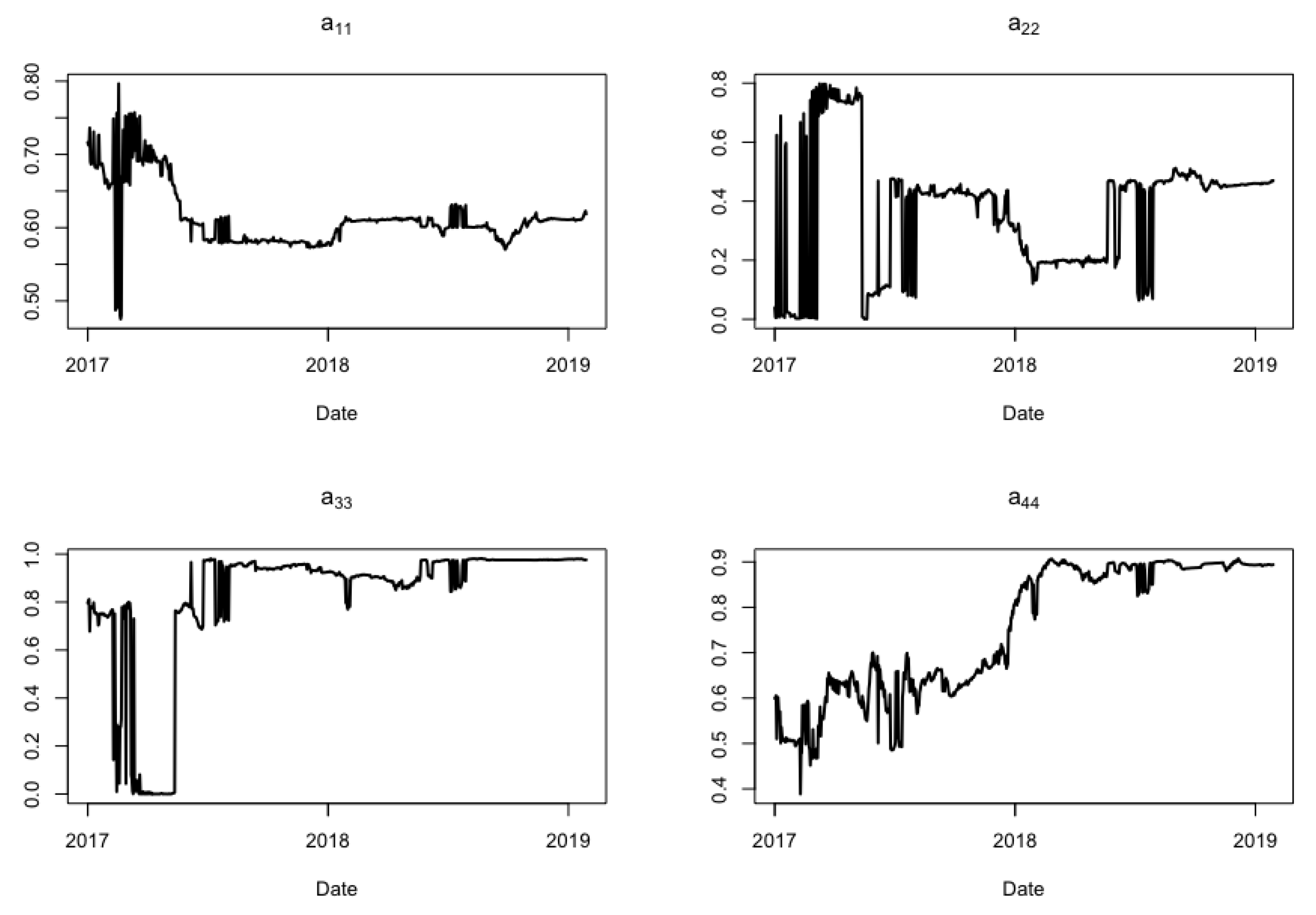
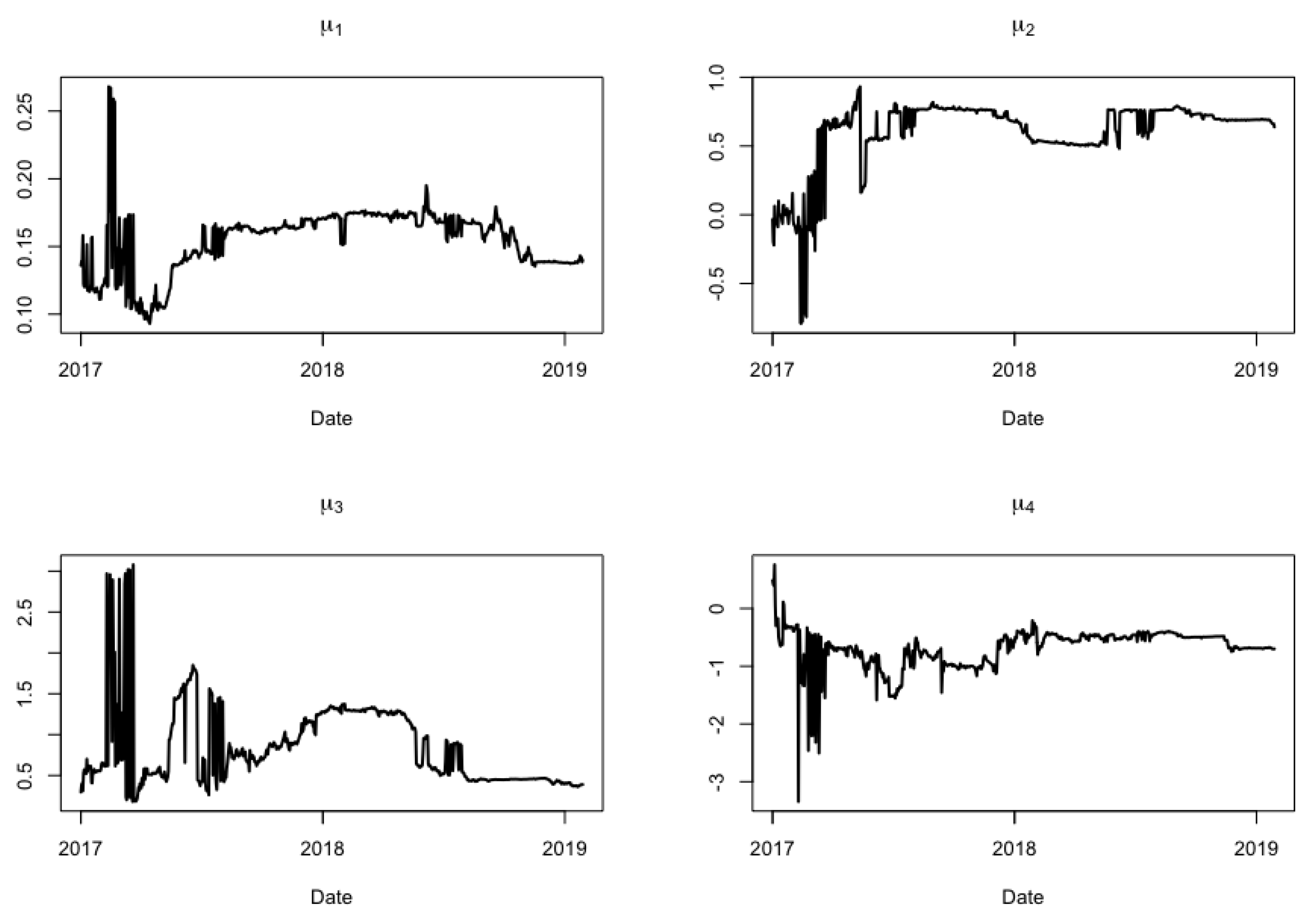
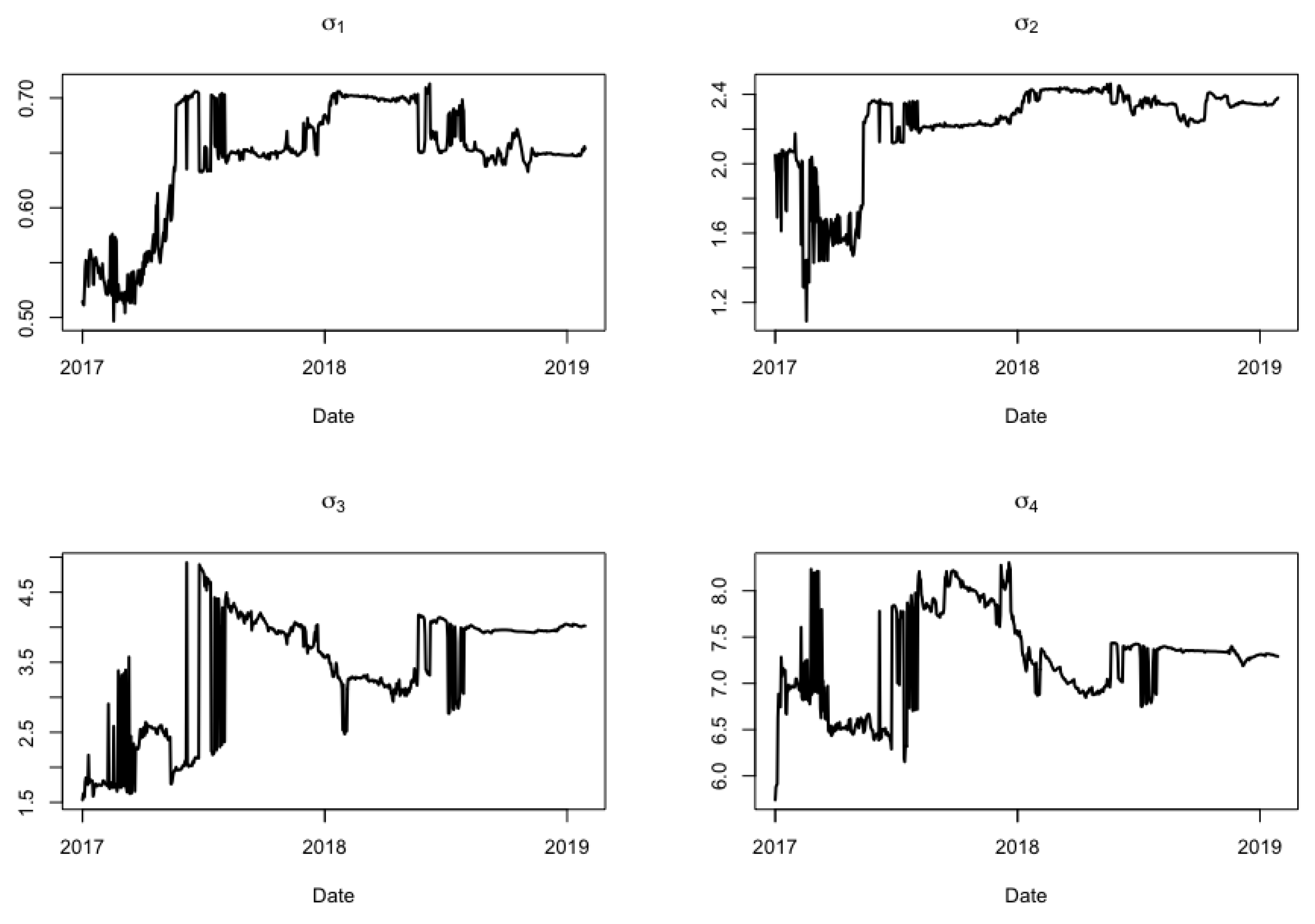
For the expanding window procedure, we shall assume that the training period is 1 January 2016–31 December 2016, while the testing period is 1 January 2017–28 January 2019. For computational stability, we shall update the model parameters and decode at each iteration in the expanding window. The test set results based on the homogeneous four-state normal HMM are given henceforth. Figure 3 shows that the probabilities of self-transition (persistence) for the states change quite drastically. Overall, the probabilities fluctuate erratically at the start of the testing period and then stabilise as more data streams in. Note that the probability of staying in the second state alternates between low and high persistence at the start of the expanding window procedure and then stabilises to medium persistence. For the third and fourth states, the probability of self-transition starts quite low but gradually increases until high persistence is achieved. Figure 4 illustrates that both means and volatilities remain quite stable. Moreover, and remain positive with low and high volatilities, respectively. For these reasons, states 1 and 3 can be considered as bull regimes, the latter being more volatile and persistent. Additionally, is negative at the start of the testing period, but it gradually becomes strongly positive. Due to the change in sign for the second state, it is not obvious whether it should be associated with a bull or bear market, and it is also associated with a weak drift. Thus, it will be considered as a correction/rally state. In contrast, state 4 retains its identity as a bear market due to the negative mean and very high volatility.
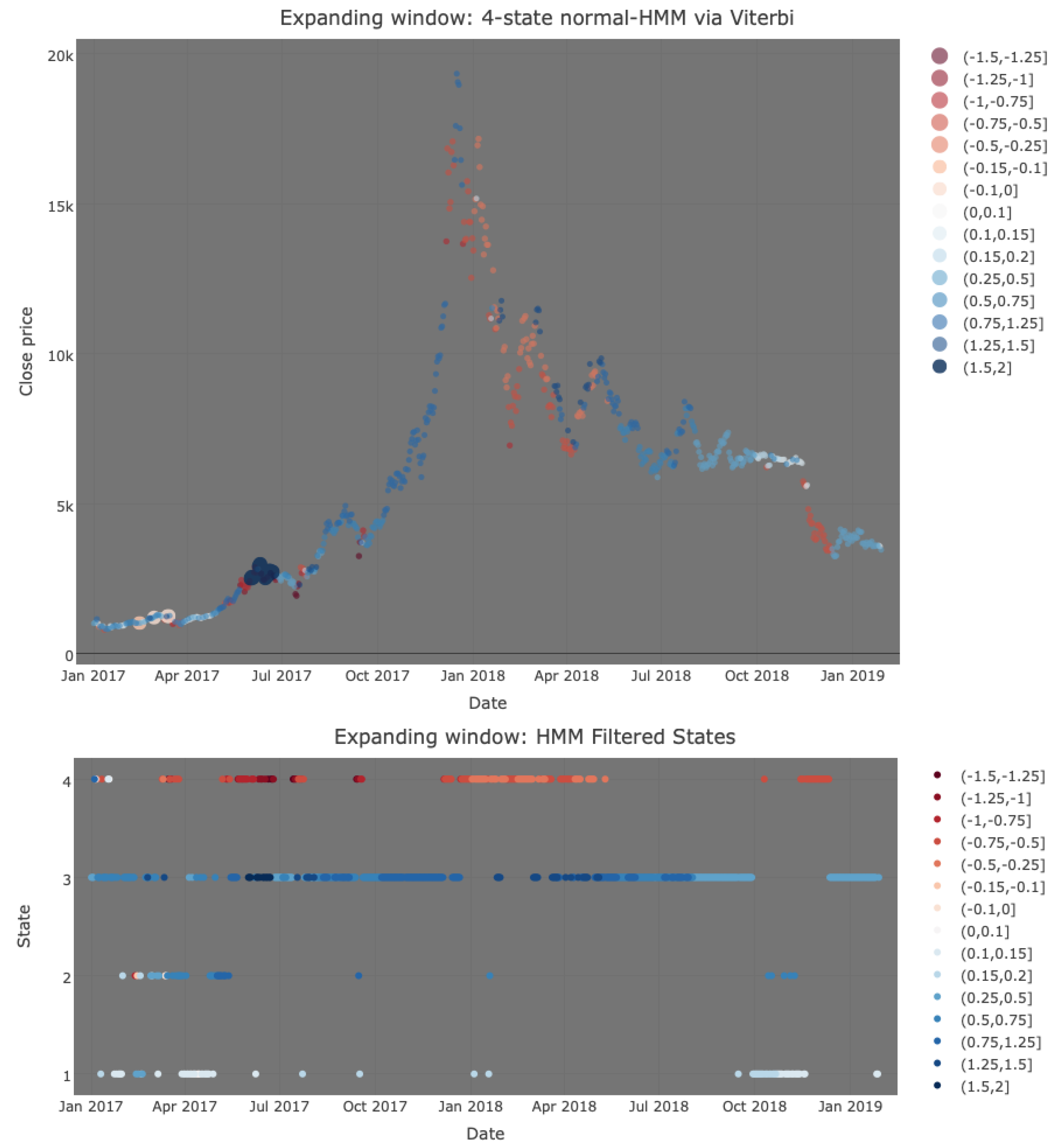
Figure 5 shows that the four-state HMM, based on a filtering method, can reasonably capture the hidden economic regimes since upward trends are generally a shade of blue, while downward trends are generally orange to red in colour. Observe that the Viterbi algorithm assigns most of the test period to the third state—the bull state. Then, at the start of 2018, the value of one Bitcoin starts plummeting, which is identified early by the Viterbi algorithm. It must be noted, though, that some minor downward trends in 2018 failed to be distinguished from upward trends. Ultimately, the four-state normal HMM seems to perform fairly well in detecting the changing market conditions.
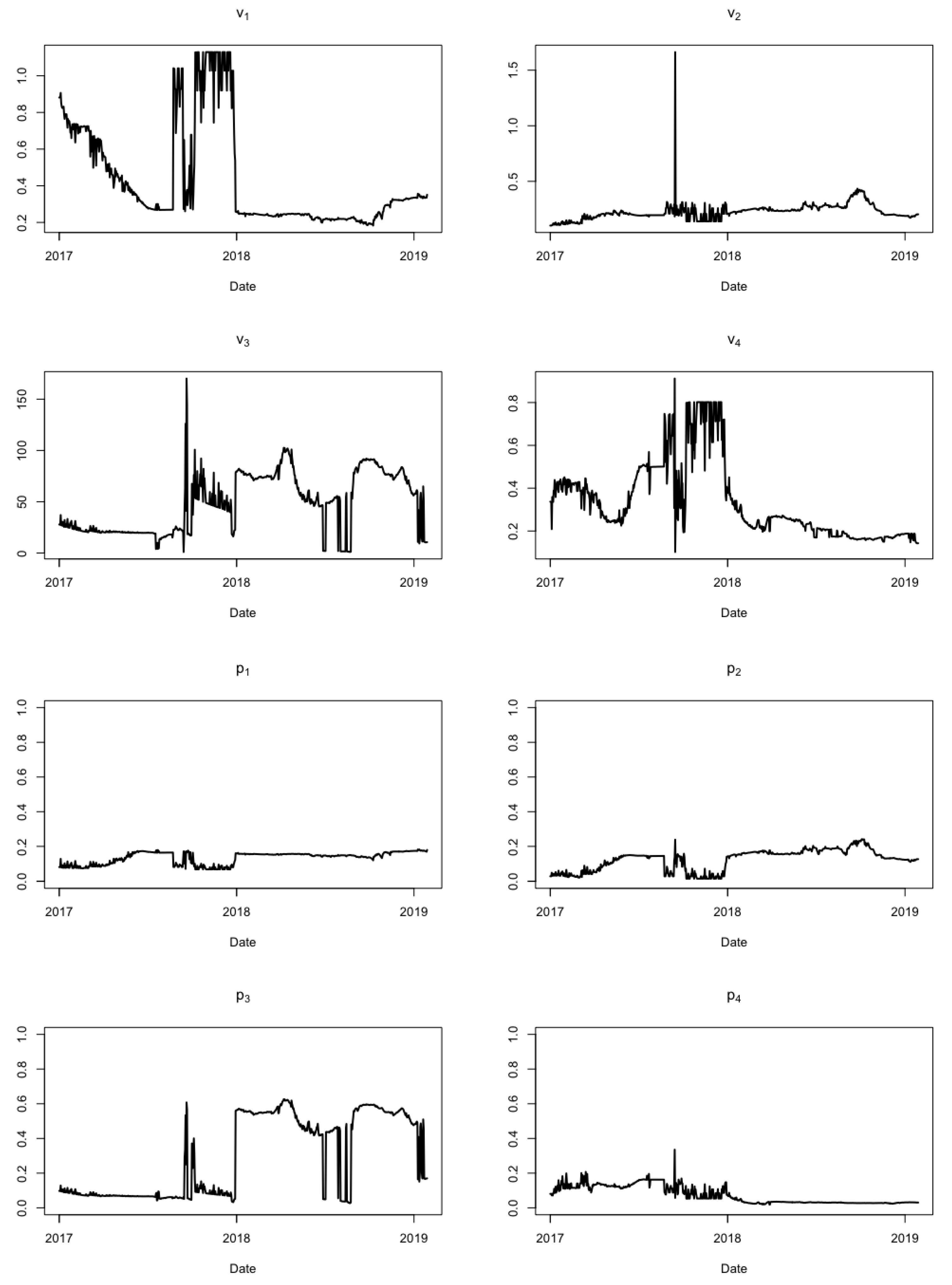
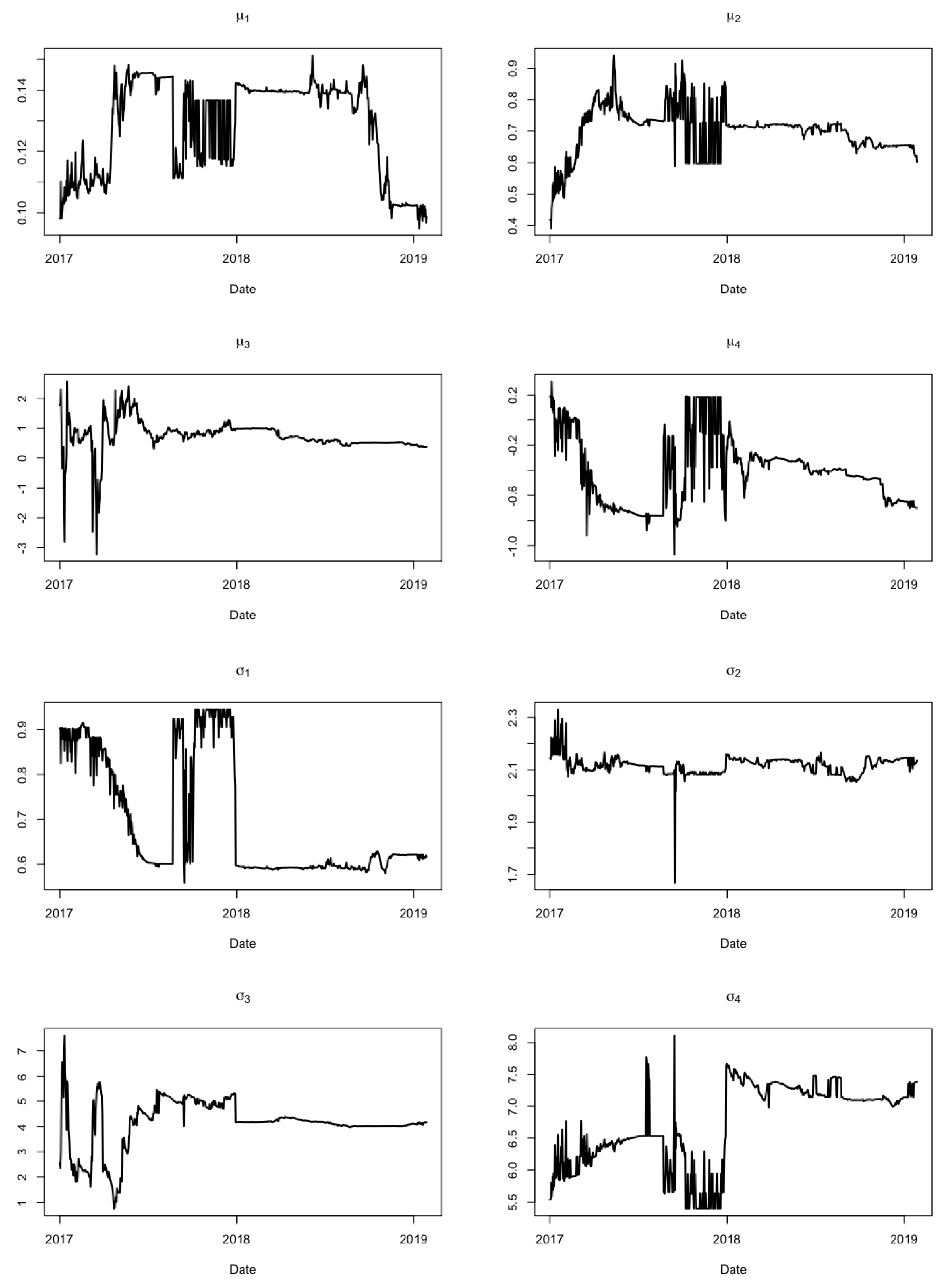
The test set results based on the homogeneous four-state normal HSMM are also presented. Figure 6 shows how the state-dependent parameters of the negative binomial distributions vary in the expanding window procedure. As can be observed, the probabilities for do not fluctuate as much as . The state-dispersion parameters, , vary substantially as more data streams in. With regards to the state-dependent normal distribution parameters (cf. Figure 7), the state means vary considerably via the expanding window procedure, especially at the end of 2017. As can be observed, such parameter estimates can be interpreted similarly to those obtained from the HMM counterpart. Moreover, the state volatilities undergo substantial changes throughout the expanding window process. Most notable is the volatility in state 3, which at the start of the testing phase is as large as the volatility in state 4.
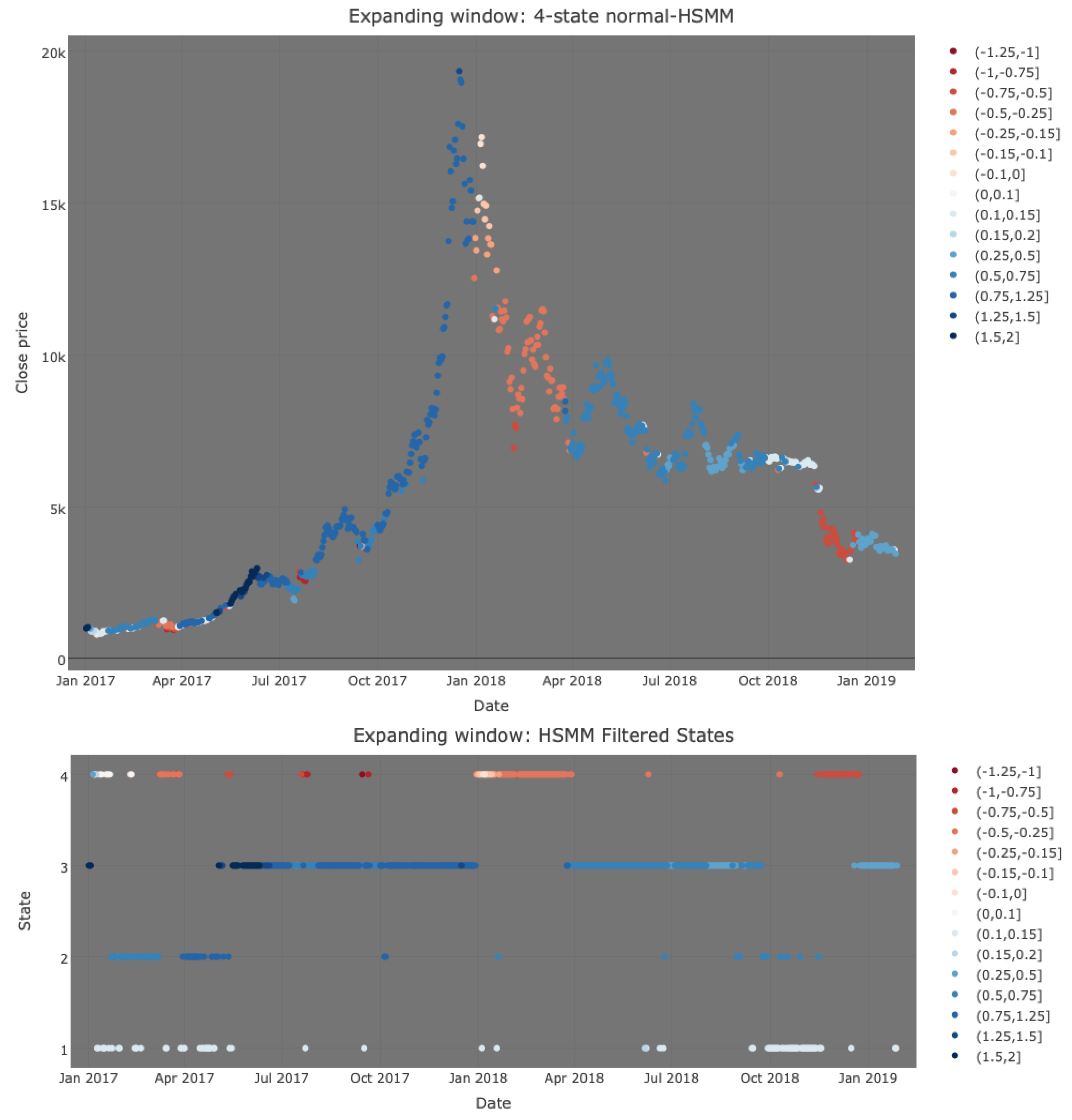
Through the use of the Viterbi algorithm, a filtering procedure was applied to infer the current hidden states, as shown by Figure 8. As can be observed, this figure differs from Figure 5, especially around the period of January 2018. In particular, it can be noted that the colours do not alternate much, which was the major criticism with the HMM based plot. Again, the Viterbi algorithm assigns most of the test period to the third state—the bull state. Then, at the start of 2018, the value of one Bitcoin starts plummeting, which is identified early by the Viterbi algorithm as state 4—the bear state. Moreover, the last days of the testing period switch between states 1 and 2. Ultimately, the four-state normal HSMM seems to perform fairly well in detecting the changing market conditions. In order to compare the market traits of BTC/USD with those of more traditional assets, we now also analyse S and P500 returns in a similar manner.
3.2. Standard and Poor 500 Index Returns
The sequence plot of S and P 500 (adjusted) close prices, , together with an illustration of the daily log returns, , can be found in Figure 9. As can be observed, the close prices exhibit periods of downward and upward trends, while the log returns are clearly characterised by volatility clustering. This observation corroborates the belief that bear markets are much more volatile than bull markets in benchmark stocks. An interesting contrast between the S and P 500 and BTC/USD emerges when noting that, for the latter, price drops and rises are highly volatile, while the former only experiences high volatility during price drops. Summary statistics of reveal that the mean and variance are equal to 0.012 and 1.457, respectively. The coefficient of skewness is negative (−0.214), implying that the distribution of log returns is left-tailed. Another stylised fact that is characterised by the series is that the coefficient of kurtosis greatly exceeds three (11.480), implying a highly leptokurtic distribution. Non-normality of the series is supported by the Jarque–Bera test (statistic: 14408, p-value: 0.00), which rejects the null hypothesis that the series follows a normal distribution at the 0.01 level of significance.
Table 4 summarises the model-fitting results on the complete series via the negative log-likelihood, AIC, BIC, and HQC for HMMs and HSMMs with different numbers of states. The DTMCs were assumed to be stationary. Note that a five-state normal HMM was also considered, but since it did not exhibit large persistence in the additional state, it was discarded. From Table 4, it can be concluded that the four-state models provide the best fit to the data, with the four-state HSMM having superiority over the four-state HMM, as demonstrated by the information criteria.
The parameter estimates and 90% confidence intervals (based on the parametric bootstrap method) for the stationary four-state normal HMM are summarised in Table 5. From the stationary probabilities, , it is evident that the four-state normal HMM spends most of its time in states 1 (38.1%) and 2 (34.0%), which are characterised by positive means and low volatilities. The least time is spent in state 4 (3.8%), which is characterised by a large negative mean and high volatility. The dynamics of the transition probabilities and state-dependent parameter estimates allow for the following interpretations of the states: (i) state 1 can be associated with a bull market due to a large positive mean with low volatility and likely transitions to states 2 and 3, (ii) state 4 can be associated with a bear market due to the large negative mean and high volatility with a likely switch to state 3, and (iii) states 2 and 3 can both be interpreted as market corrections, where the former is characterised by a positive mean with low volatility and the latter has a negative mean with larger volatility. Note that the less volatile correction state, i.e., state 2, is likely to transition to the bull state or to the more volatile correction state, i.e., state 3, while the latter can transition to the bear state or to the other correction state.
The parameter estimates and 90% confidence intervals (based on the parametric bootstrap method) for the homogeneous four-state normal HSMM, fitted via the EM algorithm, are presented in Table 6. The initial distribution estimates suggest that the series starts from state 3. The state-dependent parameter estimates closely resemble those of the four-state HMM, and thus similar interpretations can be attached to the states. Recall that the probabilities model the state switches, while the dwell-time distributions for each state, according to s and s above, model the state persistence. The negative binomial dwell-time distributions (red) are illustrated by Figure 10, which show that states clearly deviate from the geometric dwell-time distributions (black) of the aforementioned HMM.
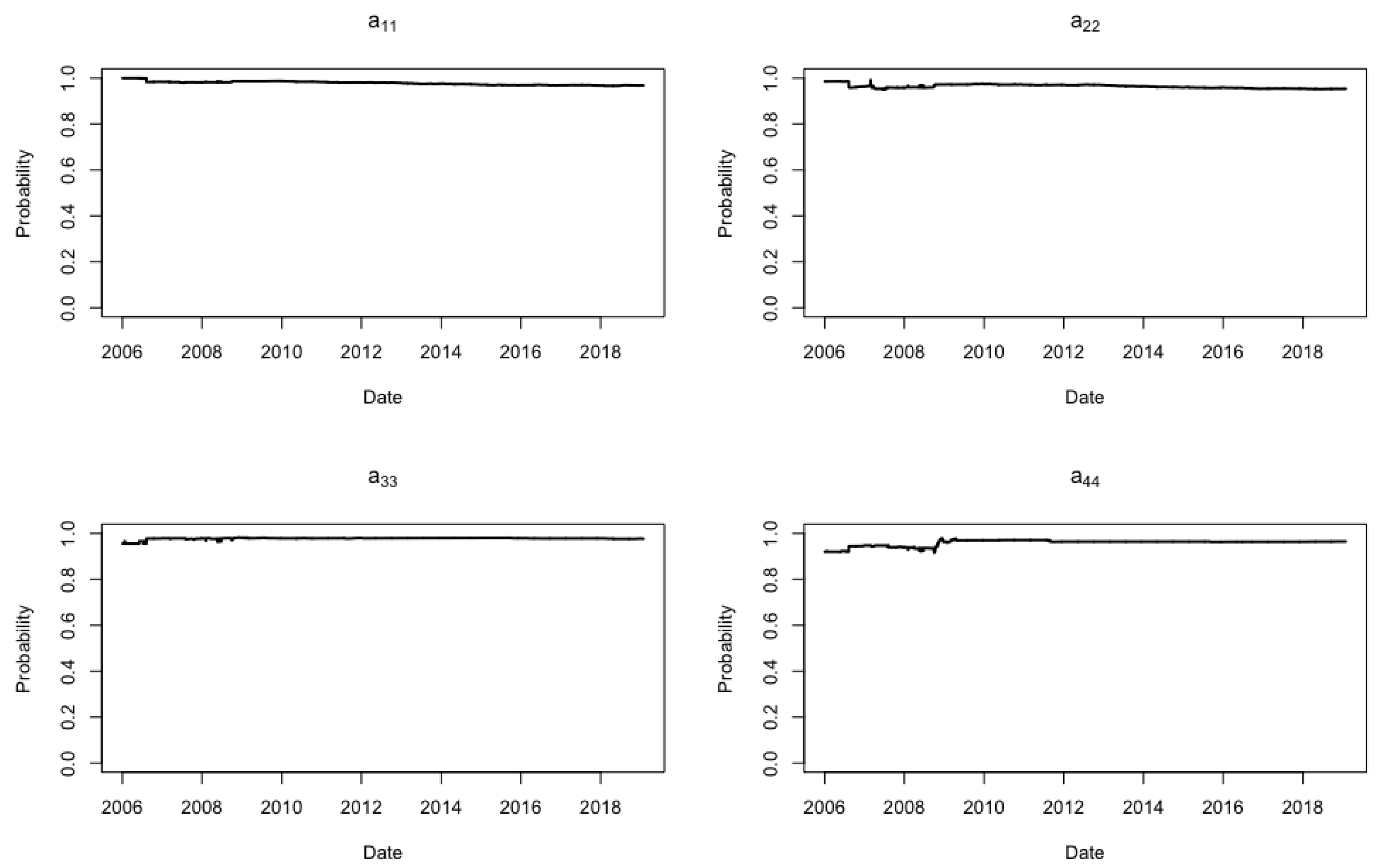
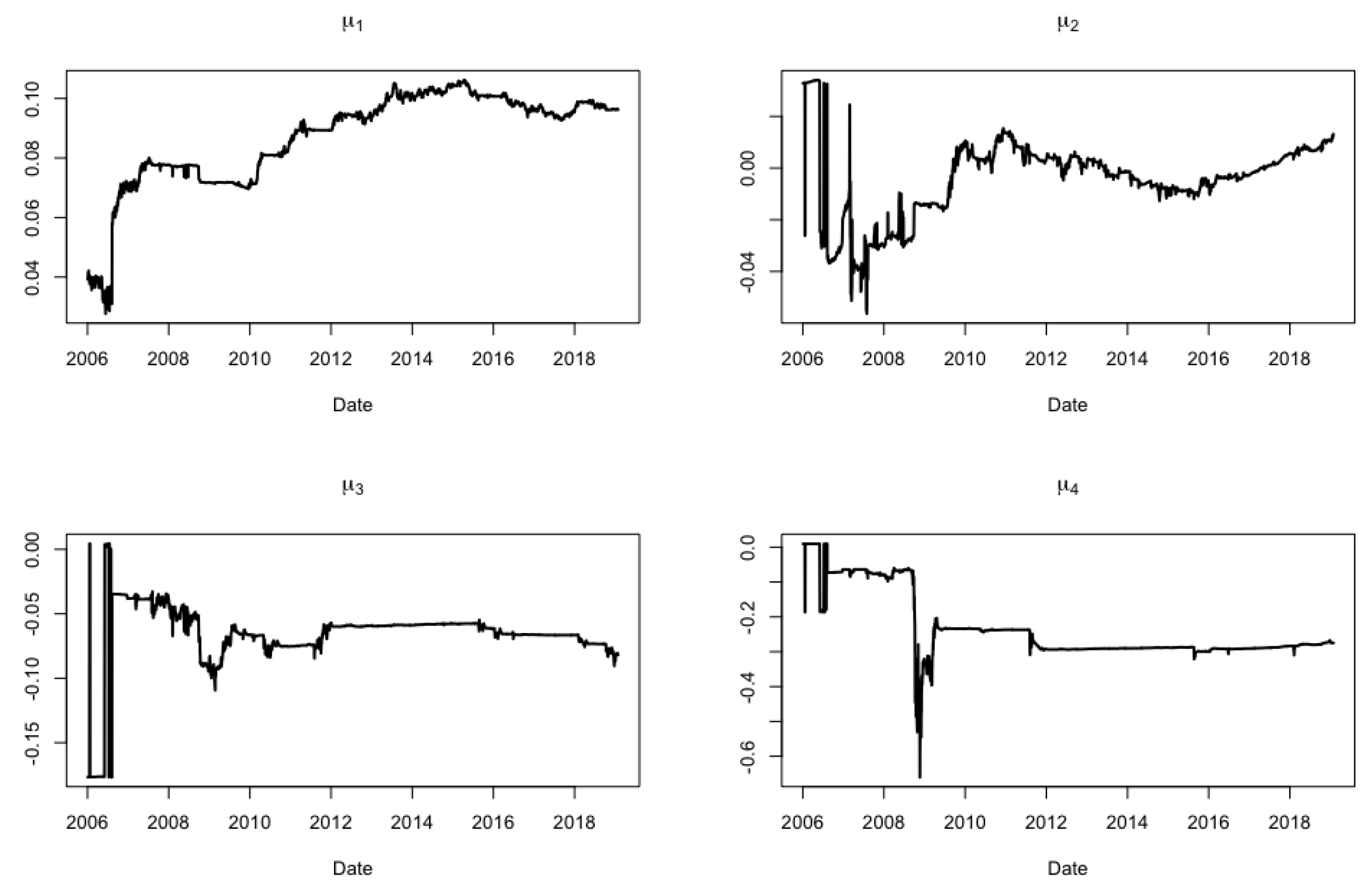
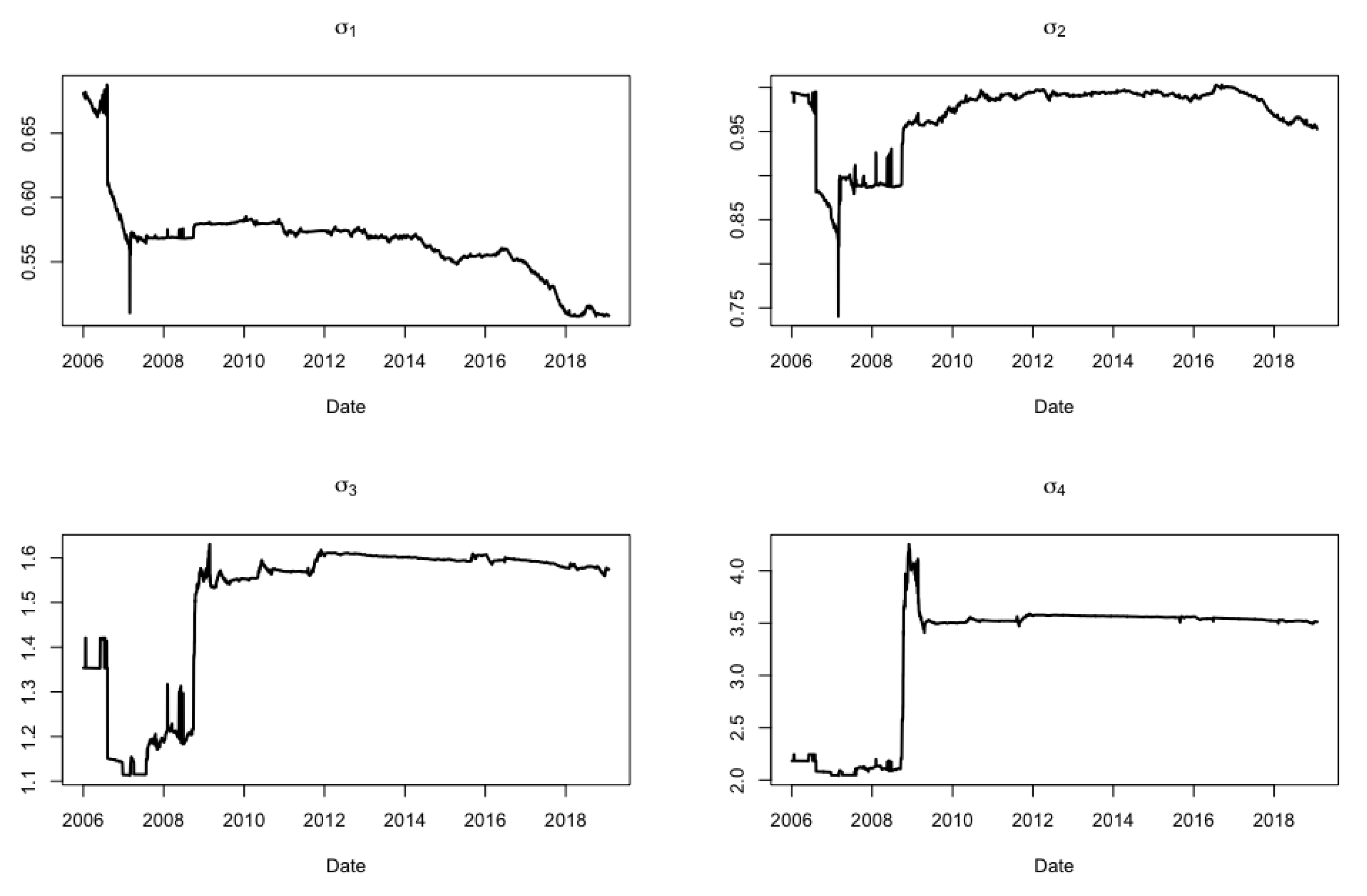
For the expanding window procedure, we shall assume that the training period is 3 January 2000–30 December 2005, while the testing period is 1 January 2006–28 January 2019. The scope of considering such a long testing period is to understand how the four-state HMM and HSMM can handle economic swings, i.e., bear vs. bull markets. We updated the model parameters and decoded at each iteration in the expanding window. The test set results based on the homogeneous four-state normal HMM are given hereafter. Figure 11 shows that the probabilities of self-transition (persistence) are close to one during the entire testing period, with little fluctuations. Figure 12 illustrates how the state-dependent parameters for the normal distributions update at each iteration of the expanding window procedure. Given estimates of , it can be observed that for all iterations. Moreover, given estimates of , note that , while for all iterations. Hence, it is clear to associate states 1 and 4 with bull and bear markets, respectively. Since and fluctuate around zero and are not consistent in their sign, it is reasonable to consider them as correction states, with their volatility being the distinguishable trait. It is interesting to note how around the period of the financial crisis of 2008, the volatilities of states 2, 3, and 4 increase sharply especially for the bear market regime. The behaviour of the state means is also similar as they fluctuate haphazardly during the 2008–2010 period and then stabilise as time goes by (more data streams in).
Figure 13 was obtained by selecting the mean and volatility of the Viterbi-chosen state at each time-point in the testing period. As can be observed, warm colours (peach to burgundy) are associated with negative means, while cool colours (pale blue to navy) are associated with positive means. Figure 13 shows that the four-state HMM, based on a filtering method, can accurately capture the dynamics of bull and bear markets since upward trends are generally blue while downward trends are generally red. Note how during the period 2010–2015, the S and P 500 Index is on the rise, with a few short periods of drops in price highlighting market corrections. These instances are captured by the four-state HMM as very pale (sometimes white) colours, implying a mean that is very close to zero, with moderate volatility (state 2). In conclusion, the HMM seems to be useful in the early detection of changing market conditions.
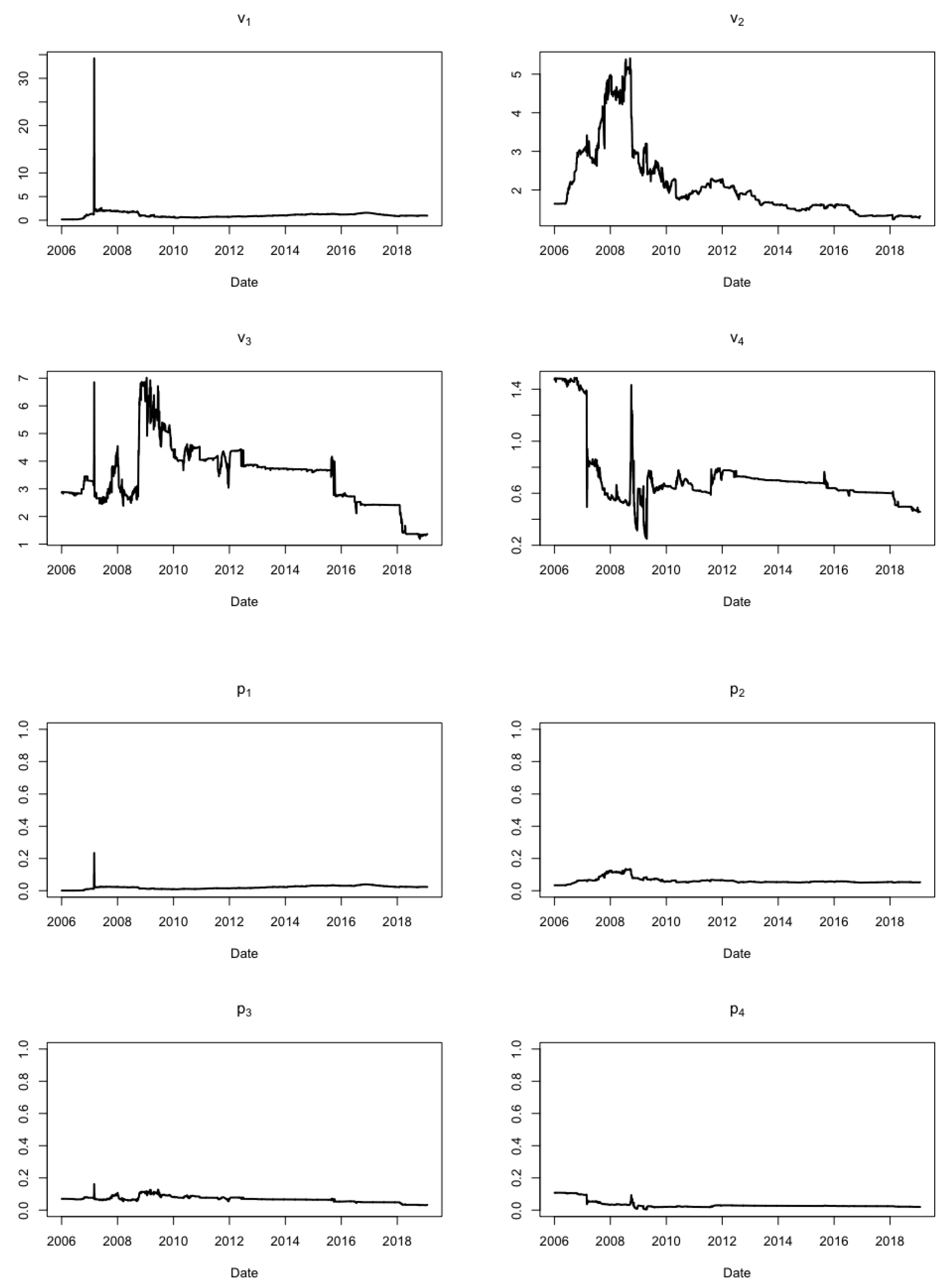
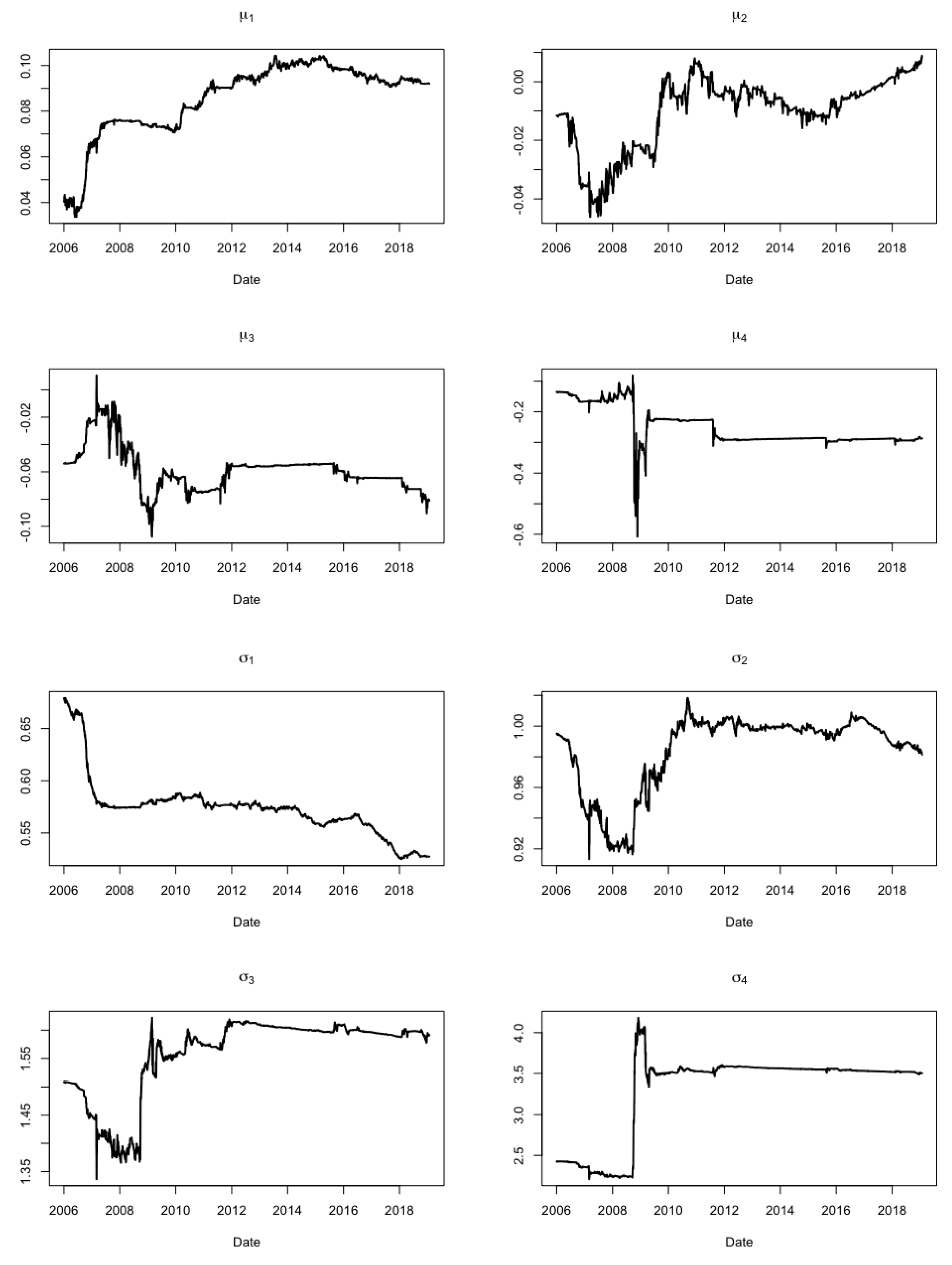
The test set results based on the homogeneous four-state normal HSMM are given hereafter. Figure 14 shows how the state-dependent parameters of the negative binomial distributions vary in the expanding window procedure. As can be observed, the probabilities do not fluctuate as much as the dispersion parameters . Figure 15 illustrates how the state-dependent normal distribution parameters change over time via the expanding window procedure. As can be observed, the parameter estimates are updated similarly to the state-dependent parameter estimates for the four-state HMM (cf. Figure 12). Therefore, similar interpretations can be attached to the four-state HSMM.
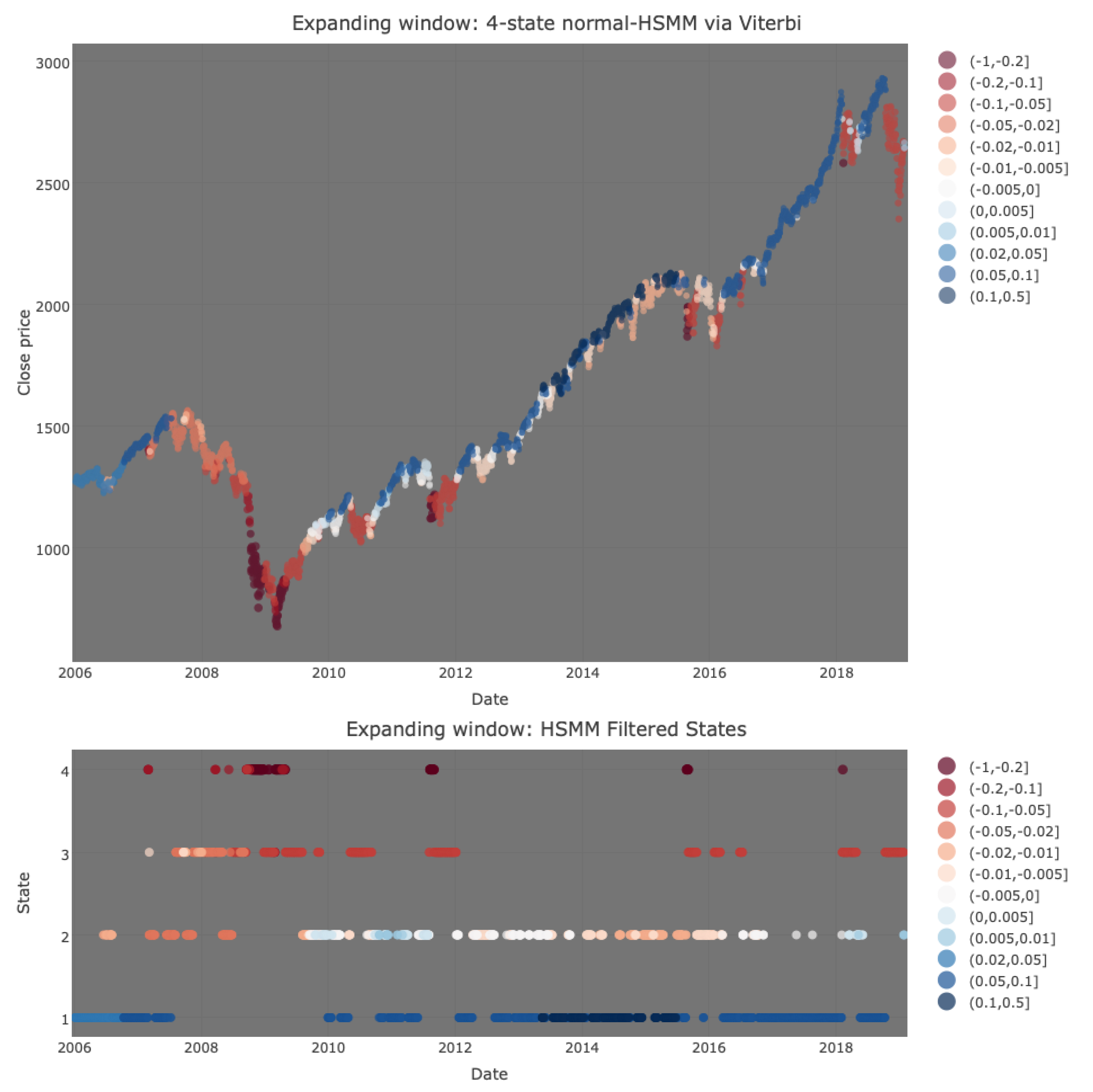
Through the use of the Viterbi algorithm, a filtering procedure was applied to infer the current hidden state, as shown by Figure 16. Upon inspection, there do not seem to be any clear differences between Figure 16 and Figure 13. Again, the four-state normal HSMM seems to capture the market dynamics well. The subtle differences between the two plots will be exploited through the implementation of investment strategies.
4. Investment Strategies to Assess Model Adequacy
In order to analyse the success of HMMs and HSMMs in determining bull and bear features, we devised four mock investment strategies and applied them with the expanding window procedure on both BTC/USD and the S and P 500, using the buy-and-hold strategy as a benchmark. For simplicity, the following assumptions were made for each strategy: (i) the actions (buy or sell) are not subject to transaction costs; (ii) the testing period is entered with an initial capital of $20,000; (iii) the first action is to buy on the first day of the testing period; (iv) if a buy signal is given, financial assets are bought only if enough cash is at hand; and (v) if a sell signal is given, financial assets are sold in their entirety if and only if they are owned. The first is a naive investment strategy called buy-and-hold, which is used for comparative purposes.
Strategy 1—Buy-and-Hold:
The buy-and-hold is defined by two actions:
- Buy on the first day of the testing phase.
- Sell on the last day of the testing phase.
The second strategy is based on the way we arbitrarily associate the states obtained via the Viterbi algorithm under the expanding window procedure (see earlier explanations for more detail).
Strategy 2—Regime:
At each state change given a particular time n, apply the following actions:
- Given that state is associated with a bear market at time and state associated with a bull market at time n, buy as many financial positions as possible at time n.
- Given that state is associated with a bull market at time and state associated with a bear market at time n, sell all financial positions at the close price of time n.
- Otherwise, do nothing.
For Bitcoin, we consider state 3 as a bull state and state 4 as a bear state, while other states will not be labelled since they are ambiguous and infrequent. For the S and P 500, on the other hand, we shall consider states 1 and 2 as bull states and states 3 and 4 as bear states, based on the probabilities in connecting them. For the third and fourth strategies below, on the other hand, we denote the mean estimate by such that is the Viterbi chosen state at time n. Moreover, the following grid values for , based on empirical evidence, are taken: ; and , for BTC/USD and the S and P 500, respectively.
Strategy 3:
Given a particular time n, apply the following actions based on a pre-specified tolerance :
- If and for , then buy as many financial positions as possible at time n.
- If and for , then sell all financial positions at the close price of time n.
- Otherwise, do nothing.
Strategy 4:
Given a particular time n, apply the following actions based on a pre-specified tolerance :
- If , and for , then buy as many financial positions as possible at time n.
- If , and for , then sell all financial positions at the close price of time n.
- Otherwise, do nothing.
Note that strategies 2 to 4 are HMM/HSMM-based since they make use of the underlying hidden states or the active state-dependent normal distribution means. Strategy 2 can be interpreted as the simplest out of the HMM/HSMM-based approaches since it only considers information regarding the inferred hidden state sequence and the “subjective” interpretations attached to each state. Strategy 3 can be interpreted as an indicator of when a regime that is characterised by a negative trend is superseded by another regime that is characterised by a positive trend, according to some pre-defined threshold value . When , strategy 3 becomes a simple indicator of a negative-to-positive trend or vice versa. Thus, this strategy tries to capture bull–bear movements and capitalise immediately on such transitions. However, strategy 3 with is clearly susceptible to market correction traps since it does not consider the size of the trend. This led to the consideration of other that take into consideration the current estimated trend size. Thus, strategy 3 with could possibly improve upon the case when by ignoring buy (or sell) signals that are based on trends that are too close to zero. Thus, choosing an attempts to capture bull and bear phases by ignoring periods which are characterised by weak upward or downward trends that could potentially mislead investors in making unprofitable decisions. However, the aforementioned strategies are flawed in situations where state-switches occur in (unrealistic) short terms. As an attempt to limit this, we considered strategy 4, which builds upon strategy 3 by additionally taking into account the trend of the day before yesterday and waiting one day before performing an action. The one-day waiting time in a particular regime acts to safeguard excessive actions during turbulent periods where the models infer consecutive (unrealistic) state-switches.
4.1. BTC/USD Exchange Rate
Table 7 summarises the pay-offs according to the aforementioned investment strategies for BTC/USD, respectively. It includes the naive buy-and-hold approach as well as the HMM and HSMM-based strategies. As can be observed for HMM-based results, strategy 4 with yields the highest ROI when compared with the other HMM-based strategies. Although strategy 4 with is almost just as profitable, notice that it requires two more actions. Thus, if transaction costs were considered, the latter strategy would suffer a hefty penalty and would not be as close to strategy 4 with . Meanwhile, for HSMM-based results, strategy 3 yields the highest ROI when compared with the other HSMM-based strategies. Note that strategy 2 yields a high return with 14 less actions. It can be concluded that the buy-and-hold strategy performs the worst but requires the lowest amount of actions. This could be attributed to the fact that the testing period under consideration was short. The overall best strategy is HSMM-based with an ROI that is more than double that of strategy 1.
Figure 17 illustrates the actions taken based on the best HSMM strategy. As can be observed, since strategy 3 is triggered whenever the mean changes from positive to negative and vice-versa, there are many actions taken throughout the testing period. Note how the HSMM-based approach was overall profitable over the testing period and made most profit by buying 13.20 BTC on 21 September 2017 and then selling them on 30 December 2017 at around $12,500 each. However, due to the declining period between April 2018 and January 2019, the model ends up making some substantial losses.
4.2. S and P 500 Index
Table 8 summarises the payoffs according to the four investment strategies for the S and P 500, respectively. As can be observed for HMM-based results, strategy 4 with yields the highest ROI when compared with the other HMM-based strategies. Although strategy 3 with is almost just as profitable, notice that it requires 36 more actions. Thus, if transaction costs were considered, the profitability in comparison to strategy 4 with would be even less. For HSMM-based results, strategy 3 with yields the highest ROI when compared with the other HSMM-based strategies. Although strategy 3 with yields the most profit, notice that it requires 16 actions, while strategy 3 with and strategy 4 with yield very similar results but with four fewer actions each. Thus, if transaction costs had been included, it is very likely that the latter would be more profitable than the former. By considering Table 8, the buy-and-hold strategy works very well. This could be attributed to the fact that the testing period under consideration is long. In spite of this, the HSMM with strategy 3 () is the most profitable under the assumed circumstances for the S and P 500 Index.
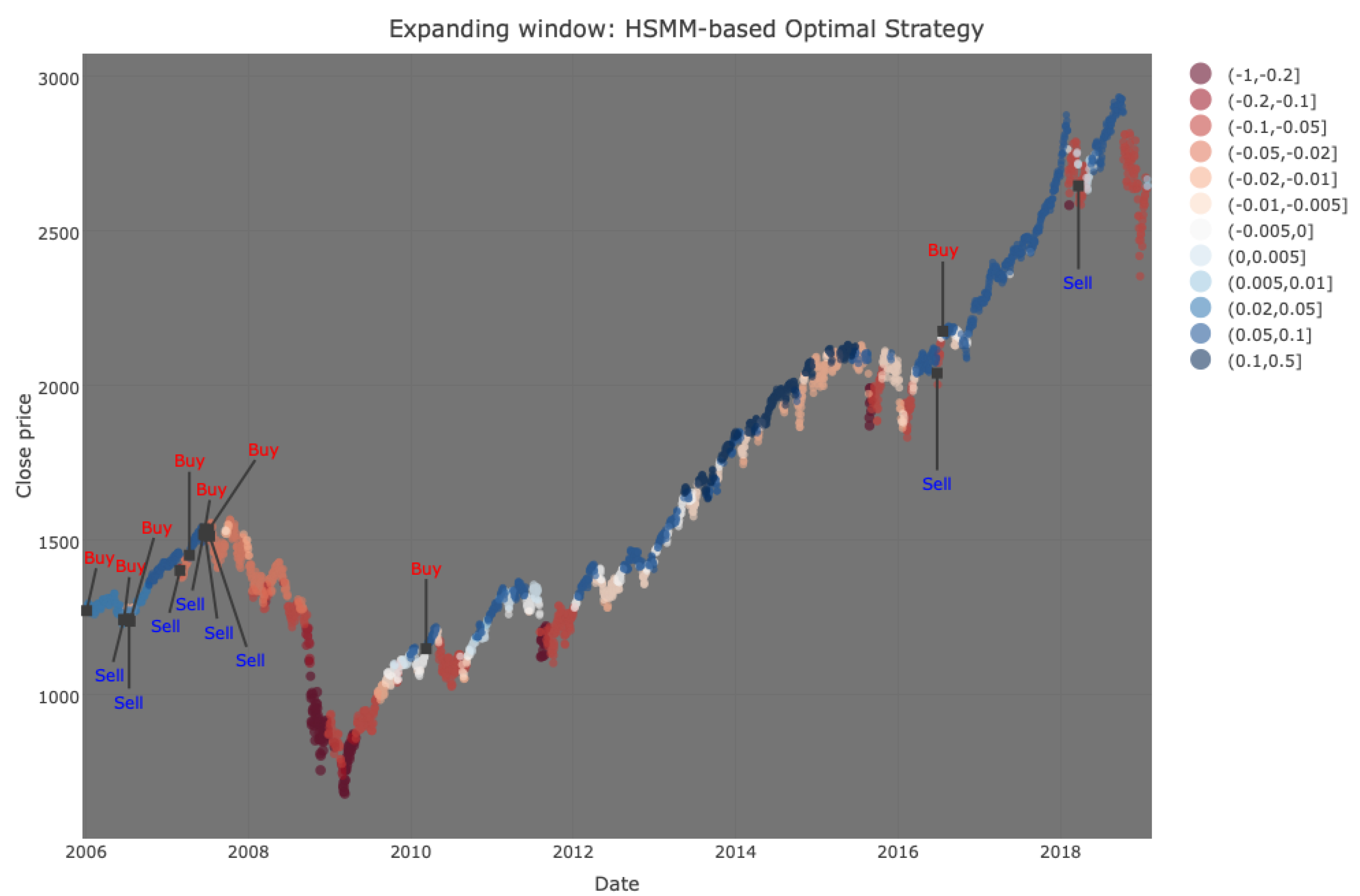
Figure 18 illustrates the actions taken based on the best HSMM strategy. As can be observed, most of the actions take place at the start of the testing period. This could be due to the fact that the parameter estimates would still be updating quite erratically during the early part and stabilise as more data streams in. Note how the HSMM-based approach anticipated the collapse during the financial crisis of 2008 and made substantial profit by holding the asset for a long time until selling in 2016.
5. Discussion
Given the results from previous sections, we now compare and contrast the features for both BTC/USD and the S and P 500. The four-state HSMMs, in both cases, reveal two states indicative of bull and bear behaviour, with two “in-between” states. However, while BTC/USD has had strong and persistent bull phases with savage and weakly persistent bear phases, for the most part, the S and P 500 tended to switch between bull and stable/bull correction phases with rare but persistent bear phases. In addition, BTC/USD can exhibit higher volatility in comparison to the S and P 500 as it is more novel and prone to external events. Indeed, both bull and bear markets for BTC/USD are volatile, while for the S and P 500, only bear markets are volatile. In view of this, cryptocurrencies have often been remarked to be excessively volatile and subject to speculation, even compared to benchmark stocks, and not currency-like in their behaviour. Secondly, BTC/USD states are less interpretable in terms of market phases than the S and P 500. While our models seem to perform well in detecting the bear states, for BTC/USD it is harder to distinguish between bull phases and more stable ones. For the S and P 500, on the other hand, steep upward trends are associated with the lowest volatility, while steep downward trends tend to be the most volatile. Ultimately, the four-state HSMM appears to be an effective modelling framework for both BTC/USD and the S and P 500.
The investment strategies results yield some notheworthy revelations. Firstly, the naive buy-and-hold strategy for the considered testing periods worked fairly well for the S and P 500, while it was the least profitable for BTC/USD, though this is largely due to the test period considered. Secondly, the HSMM framework provides a clear improvement over the standard HMM methodology in both the cryptocurrency and stock markets. Thirdly, it must be noted that for the better-performing HSMM, allowing the interpretations of the states to adjust at each step according to the mean of the state can have its advantages, as either strategy 3 or 4 improved upon strategy 2. Finally, had we considered transaction costs, it is very likely that the HSMM framework could still result in being the most profitable due to its superior performance with a relatively smaller number of transaction costs, highlighting its applicability in real-world algorithmic trading analyses.
6. Materials and Methods
The data for BTC/USD is freely available and can be downloaded from https://finance.yahoo.com/quote/BTC-USD/history?p=BTC-USD, and similarly for the S and P 500. The computer codes used to derive the results in this paper can be found as open access on https://github.com/lukespi/HMMHSMMBitcoinSP500.
7. Conclusions
In summary, this paper concludes that a more desirable approach for modelling both BTC/ USD and the S and P 500, and capturing effectively the dynamics of bull and bear market regimes, is a four-state normal HSMM with negative binomial dwell-time distributions. When implementing investment strategies, it has proven to be considerably superior to a buy-and-hold approach for our data, while this was not always the case for HMMs, which constrain dwell-times to being geometric. Indeed, by allowing dwell-time distributions on the states with larger modes, the number of buy/sell actions is greatly reduced in comparison. Although in the case of BTC/USD, the states of the four-state HSMM model have an inferior interpretation compared to the S and P 500, it still provides a good basis for further improvement and future research.
This research does have some limitations, primarily the length of the BTC/USD time series (around three years long), which was chosen as such to reflect more recent interesting times. This is not the case for the S and P 500, and one must pinpoint that this is a much older financial instrument with consistent long-term behaviour, while Bitcoin and other cryptocurrencies may still be maturing. A second limitation is that this paper has considered daily data, and the analysis may respond too late to sudden large changes in the market. In future, it may be interesting to study how such models perform in high-frequency scenarios. Two other limitations are the fact that prior specification of the number of states is required by both HMMs and HSMMs, even though these may vary throughout the test set, and the fact that transaction costs are not included in the investment strategies. The final limitation we conclude with is that only normal HMMs and HSMMs were considered, which means that the individual states are only being defined by their mean and variance. If other, more complex, distributions were considered, other features such as skewness and kurtosis of returns could also be determined. However, it is envisaged that numerical instability can be an issue with more complex models, as one seeks to estimate more parameters.
Author Contributions
Conceptualisation, D.S.; methodology, D.S. and L.S.; software, L.S.; validation, D.S. and L.S.; formal analysis, D.S. and L.S.; investigation, D.S. and L.S.; resources, D.S. and L.S.; data curation, D.S. and L.S.; writing—original draft preparation, D.S. and L.S.; writing—review and editing, D.S. and L.S.; visualisation, L.S.; supervision, D.S.; project administration, D.S.; funding acquisition, L.S.
Funding
The research work disclosed in this publication is partially funded by the Endeavour Scholarship Scheme (Malta). Scholarships are partly financed by the European Union—European Social Fund (ESF)—Operational Programme II—Cohesion Policy 2014–2020, “Investing in human capital to create more opportunities and promote the well-being of society”.
Conflicts of Interest
The authors declare no conflict of interest.
Abbreviations
The following abbreviations are used in this manuscript:
| AIC | Akaike information criterion |
| BIC | Bayesian information criterion |
| BTC/USD | Bitcoin/US dollar |
| C.I. | Confidence intervals |
| CSI 300 | Chinese Stock Index 300 |
| DNM | Direct numerical maximisation |
| DTMC | Discrete-time Markov chain |
| DTSMC | Discrete-time semi-Markov chain |
| EM | expectation maximisation |
| GARCH | Generalised autoregressive conditional heteroscedasticity |
| HMM | Hidden Markov model |
| HQC | Hannan–Quinn criterion |
| HSMM | Hidden semi-Markov model |
| MLE | Maximum likelihood estimates |
| ROI | Return on investment |
| S and P 500 | Standard and Poor’s 500 |
References
- Suda, D.; Spiteri, L. Comparing market phase features for cryptocurrency and benchmark stock index using HMM and HSMM filtering. In Lecture Notes in Business Information Processing; Springer: Berlin/Heidelberg, Germany, 2019. [Google Scholar]
- Nakamoto, S. Bitcoin: A Peer-to-Peer Electronic Cash System. Available online: www.bitcoin.org (accessed on 17 October 2019).
- ECB Crypto-Assets Task Force (European Central Bank). Crypto-Assets: Implications for Financial Stability, Monetary Policy, and Payments and Market Infrastructures; No. 223; Occasional Paper Series; European Central Bank: Frankfurt, Germany, 2019; Available online: https://www.ecb.europa.eu/pub/pdf/scpops/ecb.op223~3ce14e986c.en.pdf (accessed on 8 October 2019).
- Glaser, F.; Zimmermann, K.; Haferkorn, M.; Weber, M.C.; Siering, M. Bitcoin—Asset or currency? Revealing users’ hidden intentions. In Proceedings of the 22nd European Conference of Information Systems, Tel Aviv, Israel, 9–11 June 2014. [Google Scholar]
- Mai, F.; Shan, J.; Bai, Q.; Wang, S.; Chiang, R. How does social media impact Bitcoin value? A test of the silent majority hypothesis. J. Manag. Inf. Syst. 2015, 35, 19–52. [Google Scholar] [CrossRef]
- Yermack, D. Is Bitcoin a real currency? In The Handbook of Digital Currency, 1st ed.; Elsevier: Amsterdam, The Netherlands, 2015; pp. 31–44. [Google Scholar]
- Beer, C.; Weber, B. Bitcoin: The promise and limmits of private innovation in monetary and payment systems. Monet. Policy Econ. 2014, 4, 56–66. [Google Scholar]
- Baek, C.; Elbeck, M. Bitcoin as an investment or speculative vehicle? A first look. Appl. Econ. Lett. 2015, 22, 30–34. [Google Scholar] [CrossRef]
- Chan, S.; Chu, J.; Nadarajah, S.; Osterrieder, J. A statistical analysis of cryptocurrencies. J. Risk Financ. Manag. 2017, 10, 12. [Google Scholar] [CrossRef]
- Baur, D.G.; Dimpfl, T.; Kuck, K. Bitcoin, gold and the dollar—A replication and extension. Financ. Res. Lett. 2018, 25, 103–110. [Google Scholar] [CrossRef]
- Bouri, E.; Azzi, G.; Dyhrberg, A.H. On the return-volatility relationship in the Bitcoin market around the price crash of 2013. Econstor Econ. Discuss. Pap. 2018, 11, 2016–2041. [Google Scholar]
- Chu, J.; Chan, S.; Nadarajah, S.; Osterrieder, J. GARCH modelling of cyprtocurrencies. J. Risk Financ. Manag. 2017, 10, 17. [Google Scholar] [CrossRef]
- Katsiampa, P. Volatility estimation for Bitcoin, a comparison of GARCH models. Econ. Lett. 2017, 158, 3–6. [Google Scholar] [CrossRef]
- Stavroyiannis, S. Value-at-risk and related measures for the Bitcoin. J. Risk Financ. 2018, 19, 127–136. [Google Scholar] [CrossRef]
- Kodama, O.; Pichl, L.; Kaizoji, T. Regime change and trend prediction for Bitcoin time series data. In Proceedings of the CBU International Conference on Innovations in Science and Education 2017, Prague, Czech Republic, 22–24 March 2017. [Google Scholar]
- Ardia, D.; Bluteau, K.; Reude, M. Regime changes in Bitcoin GARCH volatility dynamics. Financ. Res. Lett. 2018, in press. [Google Scholar] [CrossRef]
- Bonello, A.; Suda, D. Volatility regime analysis of Bitcoin price dynamics using Markov switching GARCH models. In Proceedings of the 22nd European Simulation and Modelling Conference 2018, Ghent, Belgium, 24–26 October 2018. [Google Scholar]
- Hotz-Behofsits, C.; Huber, F.; Zörner, T. Predicting cryptocurrencies using sparse non-Gaussian state space models. J. Forecast 2018, 37, 627–640. [Google Scholar] [CrossRef]
- Thies, S.; Molnar, P. Bayesian changepoint analysis of Bitcoin returns. Financ. Res. Lett. 2018, 27, 223–227. [Google Scholar] [CrossRef]
- Rydén, T.; Teräsvirta, T.; Åsbrink, S. Stylized facts of daily return series and the hidden Markov model. J. Appl. Econometr. 1998, 13, 217–244. [Google Scholar] [CrossRef]
- Granger, C.W.; Ding, Z. Some properties of absolute return: An alternative measure of risk. Annales d’Economic et de Statistique 1995, 40, 67–91. [Google Scholar] [CrossRef]
- Nguyen, N. Hidden Markov Model for Stock Trading. Int. J. Financ. Stud. 2018, 6, 36. [Google Scholar] [CrossRef]
- Bulla, J.; Bulla, I. Stylized facts of financial time series and hidden semi-Markov models. Comput. Stat. Data Anal. 2007, 51, 2192–2209. [Google Scholar] [CrossRef]
- Liu, Z.; Wang, S. Decoding Chinese stock market returns: Three-state hidden semi-Markov model. Pac.-Basin Financ. J. 2017, 44, 127–149. [Google Scholar] [CrossRef] [Green Version]
- Zucchini, W.; MacDonald, I.L.; Langrock, R. Hidden Markov Models for Time Series: An introduction Using R, 2nd ed.; Chapman & Hall/CRC: Boca Raton, FL, USA, 2016. [Google Scholar]
- Guédon, Y. Estimating hidden semi-Markov chains from discrete sequences. J. Comp. Graph. Stat. 2003, 12, 604–639. [Google Scholar] [CrossRef]
- Viterbi, A.J. Error bounds for convolutional codes and an asymptotically optimal decoding algorithm. IEEE Trans. Inf. Thepry 1967, 13, 260–269. [Google Scholar] [CrossRef]
- Harte, D. R Package ’HiddenMarkov’. Version 1.8–1. 2014. Available online: http://homepages.maxnet.co.nz/davidharte/SSLIB/ (accessed on 12 March 2019).
- Bulla, J.; Bulla, I. hsmm: Hidden semi-Markov Models. R Package Version 0.4. 2013. Available online: http://CRAN.R-project.org/package=hsmm (accessed on 12 March 2019).
Figure 1.
Daily closing prices (top) and log returns (bottom) of Bitcoin/US dollar (BTC/USD) from 1 January 2016 to 28 January 2019.
Figure 1.
Daily closing prices (top) and log returns (bottom) of Bitcoin/US dollar (BTC/USD) from 1 January 2016 to 28 January 2019.
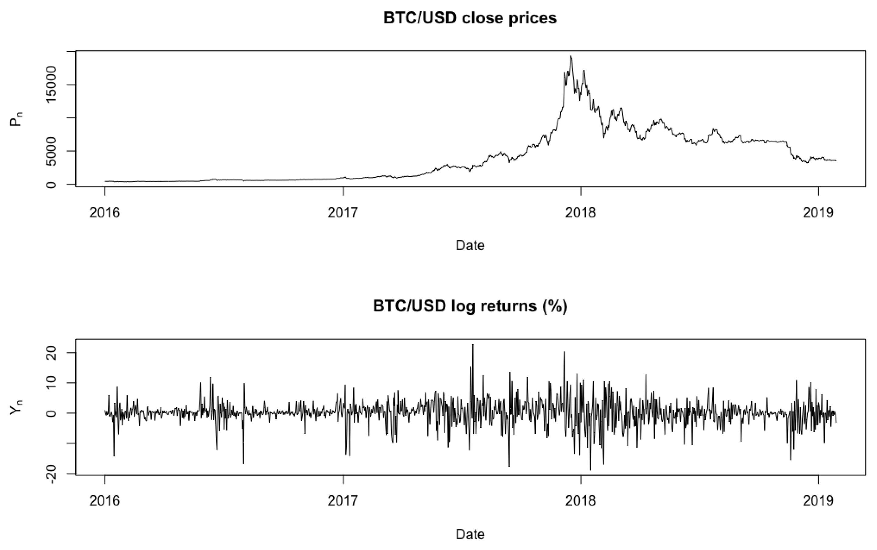
Figure 2.
State dwell-time distributions for the homogeneous four-state normal-HSMM (red) and for the stationary four-state normal-HMM (black). Figure reproduced from [1].
Figure 2.
State dwell-time distributions for the homogeneous four-state normal-HSMM (red) and for the stationary four-state normal-HMM (black). Figure reproduced from [1].

Figure 3.
Expanding window: state persistence for the homogeneous four-state normal-HMM on BTC/USD daily log returns.
Figure 3.
Expanding window: state persistence for the homogeneous four-state normal-HMM on BTC/USD daily log returns.

Figure 4.
Expanding window: state-dependent means and volatilities for the homogeneous four-state normal-HMM on BTC/USD daily log returns.
Figure 4.
Expanding window: state-dependent means and volatilities for the homogeneous four-state normal-HMM on BTC/USD daily log returns.


Figure 5.
Expanding window: four-state normal HMM filtering via the Viterbi algorithm on BTC/USD. Upper figure: Colours vary by the value of the state-dependent mean (see legend), and the larger the state-dependent volatility, the larger the dot size. Lower figure: The plot indicates the inferred state at each time-point, and the colour code also indicates the value of the state-dependent mean as per the legend. Figure reproduced from [1].

Figure 6.
Expanding window: dwell-time parameters for the homogeneous four-state normal HSMM on BTC/USD daily log returns.
Figure 6.
Expanding window: dwell-time parameters for the homogeneous four-state normal HSMM on BTC/USD daily log returns.

Figure 7.
Expanding window: state-dependent means and volatilities for the homogeneous four-state normal HSMM on BTC/USD daily log returns.
Figure 7.
Expanding window: state-dependent means and volatilities for the homogeneous four-state normal HSMM on BTC/USD daily log returns.

Figure 8.
Expanding window: four-state normal HSMM filtering via the Viterbi algorithm on BTC/USD. Upper figure: Colours vary by the value of the state-dependent mean (see legend), and the larger the state-dependent volatility, the larger the dot size. Lower figure: The plot indicates the inferred state at each time point, and the colour code also indicates the value of the state-dependent mean as per the legend. Figure reproduced from [1].

Figure 9.
Daily close prices (top) and log returns (bottom) of the S and P 500 from 1 January 2000 to 28 January 2019.
Figure 9.
Daily close prices (top) and log returns (bottom) of the S and P 500 from 1 January 2000 to 28 January 2019.
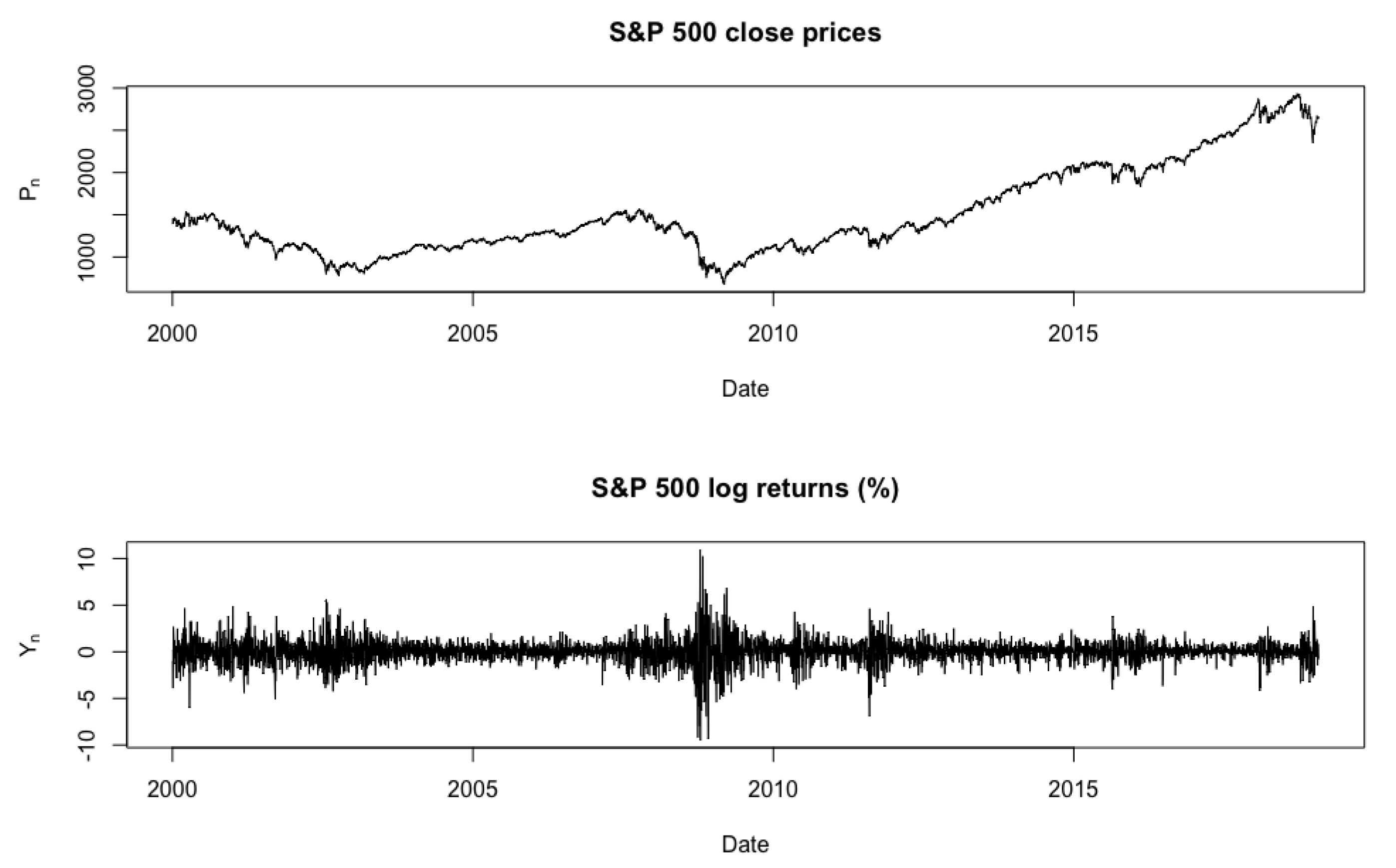
Figure 10.
State dwell-time distributions for the homogeneous four-state normal HSMM (red) and for the stationary four-state normal HMM (black). Figure reproduced from [1].
Figure 10.
State dwell-time distributions for the homogeneous four-state normal HSMM (red) and for the stationary four-state normal HMM (black). Figure reproduced from [1].

Figure 11.
Expanding window: state persistence for the homogeneous four-state normal HMM on S and P 500 daily log returns.
Figure 11.
Expanding window: state persistence for the homogeneous four-state normal HMM on S and P 500 daily log returns.

Figure 12.
Expanding window: state-dependent means and volatilities for the homogeneous four-state normal HMM on S and P 500 daily log returns.
Figure 12.
Expanding window: state-dependent means and volatilities for the homogeneous four-state normal HMM on S and P 500 daily log returns.


Figure 13.
Expanding window: four-state normal HMM filtering via the Viterbi algorithm on the S and P 500 Index. Upper figure: Colours vary by the value of the state-dependent mean (see legend), and the larger the state-dependent volatility, the larger the dot size. Lower figure: The plot indicates the inferred state at each time-point, and the colour code also indicates the value of the state-dependent mean as per the legend. Figure reproduced from [1].
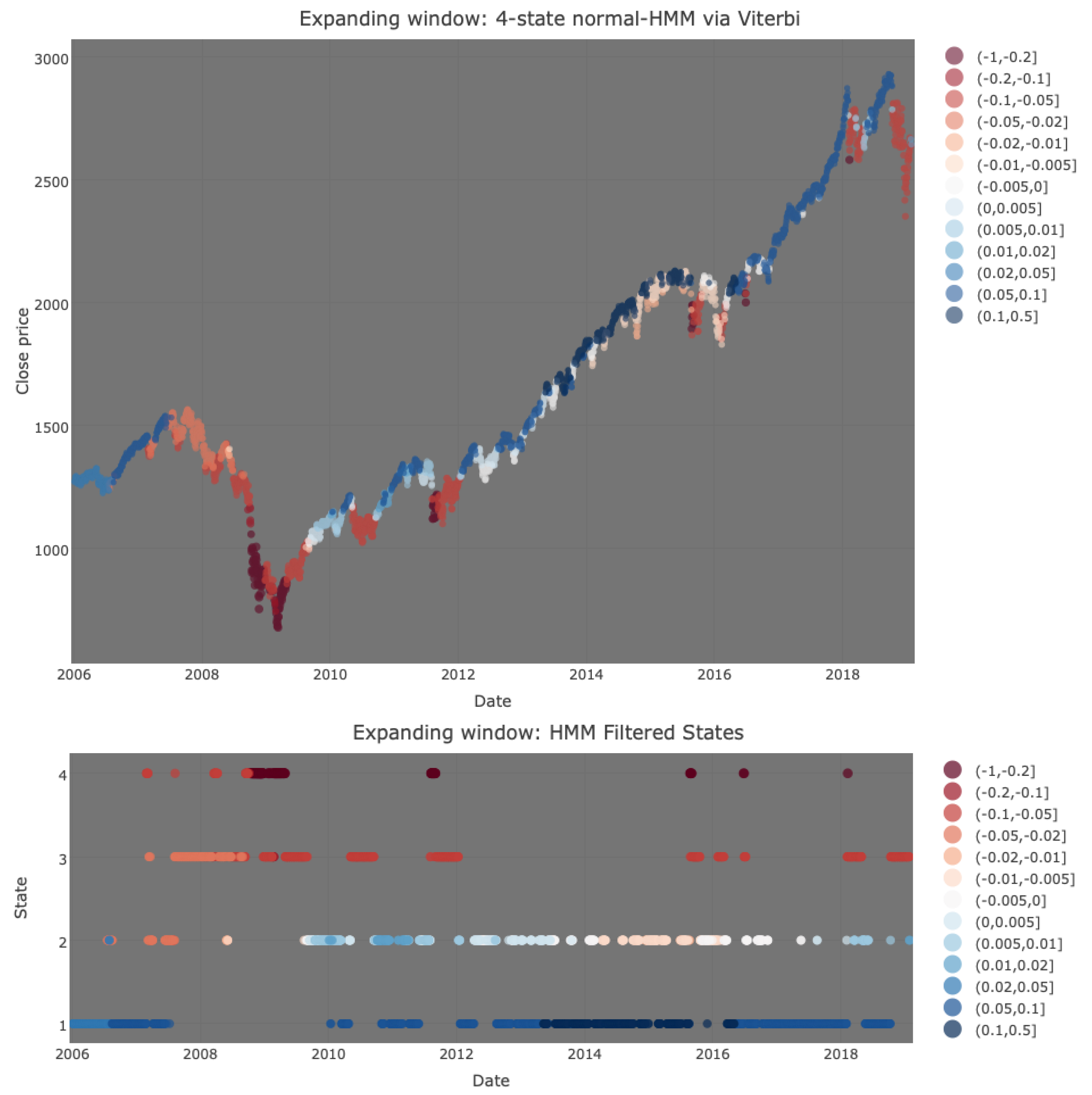
Figure 14.
Expanding window: dwell-time parameters for the homogeneous four-state normal HSMM on S and P 500 daily log returns.
Figure 14.
Expanding window: dwell-time parameters for the homogeneous four-state normal HSMM on S and P 500 daily log returns.

Figure 15.
Expanding window: state-dependent means and volatilities for the homogeneous four-state normal HSMM on S and P 500 daily log returns.
Figure 15.
Expanding window: state-dependent means and volatilities for the homogeneous four-state normal HSMM on S and P 500 daily log returns.

Figure 16.
Expanding window: four-state normal HSMM filtering via the Viterbi algorithm on the S and P 500 Index. Upper figure: Colours vary by the value of the state-dependent mean (see legend), and the larger the state-dependent volatility, the larger the dot size. Lower figure: The plot indicates the inferred state at each time-point, and the colour code also indicates the value of the state-dependent mean as per the legend. Figure reproduced from [1].

Figure 17.
HSMM-based best strategy for BTC/USD actions. Colours vary by the value of the state-dependent mean (see legend), and buy and sell signals are denoted in the figure.
Figure 17.
HSMM-based best strategy for BTC/USD actions. Colours vary by the value of the state-dependent mean (see legend), and buy and sell signals are denoted in the figure.
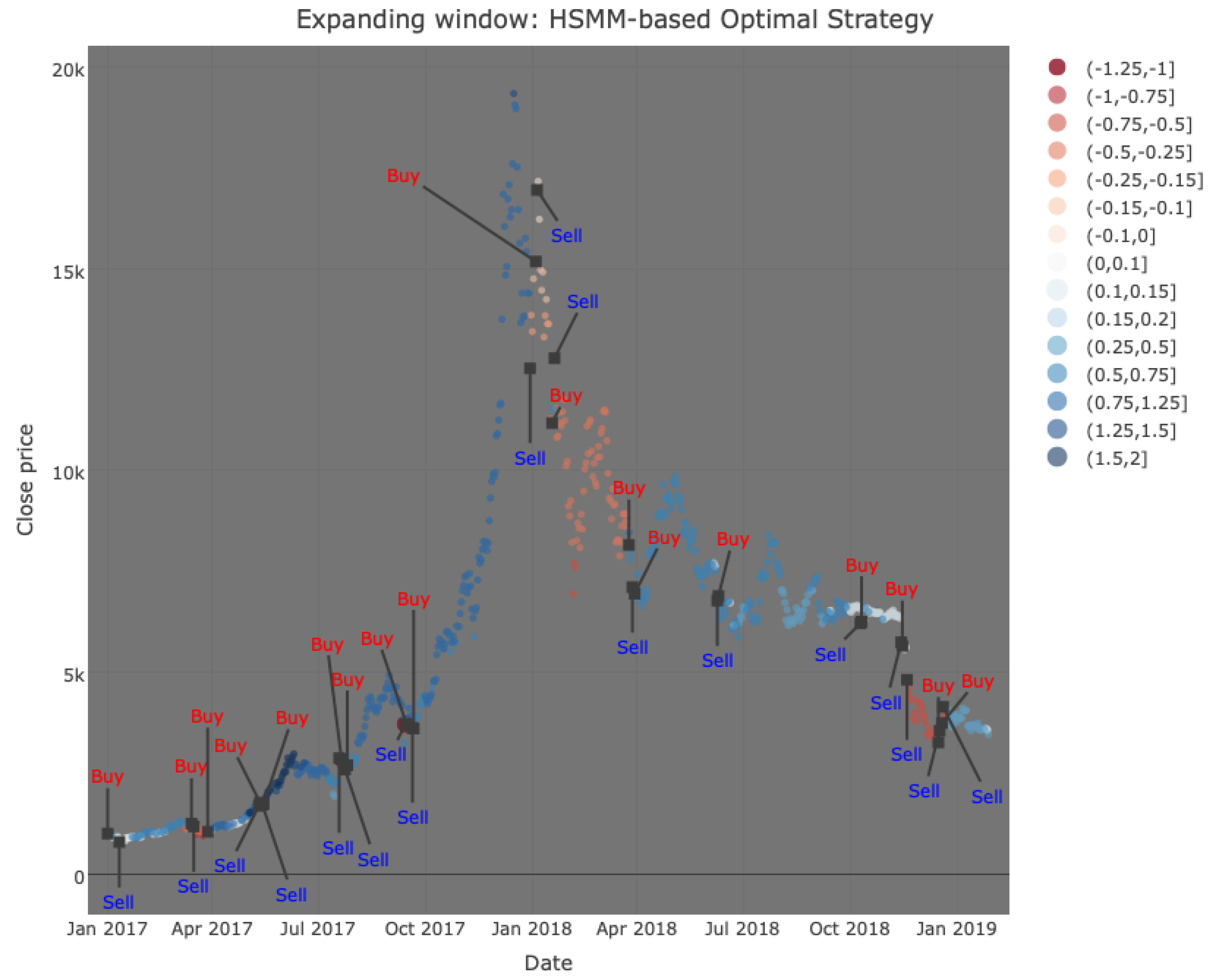
Figure 18.
Best HSMM-based strategy for S and P 500 Index actions. Colours vary by the value of the state-dependent mean (see legend), and buy and sell signals are denoted in the figure.
Figure 18.
Best HSMM-based strategy for S and P 500 Index actions. Colours vary by the value of the state-dependent mean (see legend), and buy and sell signals are denoted in the figure.


Table 1.
Goodness-of-fit statistics of stationary normal HMMs and homogeneous normal HSMMs with negative binomial dwell-time distributions for 2, 3, and 4 states based on the entire series of daily log returns of BTC/USD. Table reproduced from [1].
Table 1.
Goodness-of-fit statistics of stationary normal HMMs and homogeneous normal HSMMs with negative binomial dwell-time distributions for 2, 3, and 4 states based on the entire series of daily log returns of BTC/USD. Table reproduced from [1].
| Model | AIC | BIC | HQC | |
|---|---|---|---|---|
| 2-state HMM | 2924.454 | 5860.908 | 5891.056 | 5872.302 |
| 3-state HMM | 2872.646 | 5769.292 | 5829.587 | 5792.078 |
| 4-state HMM | 2848.546 | 5737.093 | 5837.586 | 5775.070 |
| 2-state HSMM | 2887.872 | 5779.743 | 5789.793 | 5783.541 |
| 3-state HSMM | 2857.086 | 5720.171 | 5735.245 | 5725.868 |
| 4-state HSMM | 2837.926 | 5683.852 | 5703.950 | 5691.447 |
Table 2.
Parameter estimates and parametric bootstrap confidence intervals for the stationary four-state HMM based on the complete BTC/USD log returns series.
Table 2.
Parameter estimates and parametric bootstrap confidence intervals for the stationary four-state HMM based on the complete BTC/USD log returns series.
| Parameter | MLE | 90% C.I. | |
|---|---|---|---|
| 0.275 | 0.151 | 0.356 | |
| 0.197 | 0.099 | 0.266 | |
| 0.357 | 0.207 | 0.590 | |
| 0.171 | 0.083 | 0.259 | |
| 0.616 | 0.498 | 0.712 | |
| 0.344 | 0.241 | 0.471 | |
| 0.000 | 0.000 | 0.000 | |
| 0.039 | 0.000 | 0.064 | |
| 0.537 | 0.358 | 0.769 | |
| 0.448 | 0.190 | 0.614 | |
| 0.003 | 0.000 | 0.037 | |
| 0.012 | 0.000 | 0.110 | |
| 0.000 | 0.000 | 0.000 | |
| 0.011 | 0.002 | 0.030 | |
| 0.975 | 0.944 | 0.990 | |
| 0.014 | 0.000 | 0.034 | |
| 0.000 | 0.000 | 0.000 | |
| 0.058 | 0.021 | 0.100 | |
| 0.048 | 0.016 | 0.116 | |
| 0.893 | 0.813 | 0.932 | |
| 0.142 | 0.051 | 0.216 | |
| 0.641 | 0.345 | 1.119 | |
| 0.392 | −0.024 | 0.754 | |
| −0.700 | −1.725 | 0.133 | |
| 0.661 | 0.574 | 0.759 | |
| 2.398 | 2.056 | 2.720 | |
| 4.016 | 3.662 | 4.412 | |
| 7.289 | 6.549 | 8.526 | |
Table 3.
Parameter estimates and parametric bootstrap confidence intervals for the homogeneous four-state HSMM based on the complete BTC/USD log returns series.
Table 3.
Parameter estimates and parametric bootstrap confidence intervals for the homogeneous four-state HSMM based on the complete BTC/USD log returns series.
| Parameter | MLE | 90% C.I. | |
|---|---|---|---|
| 1.000 | 0.45 | 1.00 | |
| 0.000 | 0.000 | 0.000 | |
| 0.000 | 0.000 | 0.000 | |
| 0.000 | 0.000 | 0.000 | |
| 0.831 | 0.630 | 0.953 | |
| 0.000 | 0.000 | 0.000 | |
| 0.169 | 0.047 | 0.370 | |
| 0.901 | 0.798 | 0.993 | |
| 0.000 | 0.000 | 0.000 | |
| 0.099 | 0.007 | 0.202 | |
| 0.000 | 0.000 | 0.000 | |
| 0.270 | 0.000 | 0.978 | |
| 0.730 | 0.022 | 1.000 | |
| 0.006 | 0.000 | 0.162 | |
| 0.769 | 0.406 | 0.853 | |
| 0.225 | 0.146 | 0.507 | |
| 0.351 | 0.150 | 1.232 | |
| 0.204 | 0.089 | 0.552 | |
| 10.573 | 1.854 | 83.826 | |
| 0.143 | 0.080 | 0.532 | |
| 0.180 | 0.111 | 0.365 | |
| 0.126 | 0.049 | 0.245 | |
| 0.170 | 0.043 | 0.580 | |
| 0.031 | 0.013 | 0.110 | |
| 0.099 | 0.013 | 0.190 | |
| 0.603 | 0.302 | 0.823 | |
| 0.376 | −0.006 | 0.821 | |
| −0.702 | −1.828 | 0.106 | |
| 0.617 | 0.555 | 0.693 | |
| 2.135 | 1.891 | 2.414 | |
| 4.162 | 3.900 | 4.392 | |
| 7.376 | 6.471 | 8.269 | |
Table 4.
Goodness-of-fit statistics of stationary normal HMMs and homogeneous normal HSMMs with negative binomial dwell-time distributions for 2,3, and 4 states based on the entire series of daily log returns of the S and P 500. Table reproduced from [1].
Table 4.
Goodness-of-fit statistics of stationary normal HMMs and homogeneous normal HSMMs with negative binomial dwell-time distributions for 2,3, and 4 states based on the entire series of daily log returns of the S and P 500. Table reproduced from [1].
| Model | AIC | BIC | HQC | |
|---|---|---|---|---|
| 2-state HMM | 6744.512 | 13,501.02 | 13,539.88 | 13,514.67 |
| 3-state HMM | 6536.509 | 13,097.02 | 13,174.73 | 13,124.34 |
| 4-state HMM | 6483.062 | 13,006.12 | 13,135.64 | 13,051.61 |
| 2-state HSMM | 6684.716 | 13,373.43 | 13,386.38 | 13,377.98 |
| 3-state HSMM | 6533.021 | 13,072.04 | 13,091.47 | 13,078.87 |
| 4-state HSMM | 6467.457 | 12,942.91 | 12,968.82 | 12,952.01 |
Table 5.
Parameter estimates and parametric bootstrap confidence intervals for the stationary four-state HMM based on the complete S and P 500 log returns series.
Table 5.
Parameter estimates and parametric bootstrap confidence intervals for the stationary four-state HMM based on the complete S and P 500 log returns series.
| Parameter | MLE | 90% C.I. | |
|---|---|---|---|
| 0.381 | 0.289 | 0.480 | |
| 0.340 | 0.284 | 0.423 | |
| 0.242 | 0.116 | 0.342 | |
| 0.038 | 0.01 | 0.07 | |
| 0.967 | 0.955 | 0.976 | |
| 0.031 | 0.023 | 0.042 | |
| 0.002 | 0.000 | 0.007 | |
| 0.000 | 0.000 | 0.000 | |
| 0.036 | 0.026 | 0.051 | |
| 0.953 | 0.939 | 0.965 | |
| 0.010 | 0.004 | 0.016 | |
| 0.000 | 0.000 | 0.002 | |
| 0.000 | 0.000 | 0.000 | |
| 0.018 | 0.011 | 0.031 | |
| 0.977 | 0.964 | 0.985 | |
| 0.005 | 0.002 | 0.007 | |
| 0.000 | 0.000 | 0.000 | |
| 0.000 | 0.000 | 0.000 | |
| 0.036 | 0.019 | 0.067 | |
| 0.964 | 0.933 | 0.981 | |
| 0.096 | 0.069 | 0.113 | |
| 0.013 | −0.022 | 0.055 | |
| −0.081 | −0.193 | 0.001 | |
| −0.275 | −0.804 | 0.145 | |
| 0.507 | 0.491 | 0.523 | |
| 0.951 | 0.912 | 0.987 | |
| 1.573 | 1.513 | 3.219 | |
| 3.513 | 1.657 | 3.787 | |
Table 6.
Parameter estimates and parametric bootstrap confidence intervals for the homogeneous four-state HSMM based on the complete S and P 500 log returns series.
Table 6.
Parameter estimates and parametric bootstrap confidence intervals for the homogeneous four-state HSMM based on the complete S and P 500 log returns series.
| Parameter | MLE | 90% C.I. | |
|---|---|---|---|
| 0.000 | 0.000 | 0.000 | |
| 0.000 | 0.000 | 0.000 | |
| 1.000 | 1.000 | 1.000 | |
| 0.000 | 0.000 | 0.000 | |
| 0.998 | 0.974 | 1.000 | |
| 0.002 | 0.000 | 0.026 | |
| 0.000 | 0.000 | 0.000 | |
| 0.973 | 0.954 | 0.995 | |
| 0.023 | 0.004 | 0.035 | |
| 0.004 | 0.000 | 0.014 | |
| 0.000 | 0.000 | 0.000 | |
| 0.767 | 0.571 | 0.940 | |
| 0.233 | 0.060 | 0.429 | |
| 0.000 | 0.000 | 0.000 | |
| 0.000 | 0.000 | 0.000 | |
| 1.000 | 1.000 | 1.000 | |
| 0.079 | 0.055 | 0.142 | |
| 0.112 | 0.070 | 0.226 | |
| 7.755 | 3.718 | 46.090 | |
| 0.455 | 0.156 | 5.622 | |
| 0.028 | 0.017 | 0.045 | |
| 0.044 | 0.028 | 0.098 | |
| 0.119 | 0.052 | 0.473 | |
| 0.015 | 0.012 | 0.158 | |
| 0.107 | 0.085 | 0.132 | |
| 0.000 | −0.047 | 0.045 | |
| −0.119 | −0.121 | 0.011 | |
| 0.015 | −0.829 | 0.253 | |
| 0.449 | 0.427 | 0.470 | |
| 0.970 | 0.924 | 1.022 | |
| 1.540 | 1.479 | 1.591 | |
| 3.385 | 2.885 | 3.959 | |
Table 7.
Investment metrics for buy-and-hold and HMM- and HSMM-based strategies during the testing period of 1 January 2017–28 January 2019 for BTC/USD. Best strategy marked in bold.
Table 7.
Investment metrics for buy-and-hold and HMM- and HSMM-based strategies during the testing period of 1 January 2017–28 January 2019 for BTC/USD. Best strategy marked in bold.
| Strategy | Number of Actions | Last Sell Date | Cumulative Amount ($) | ROI (%) | |
|---|---|---|---|---|---|
| 1 (Buy-and-Hold) | / | 2 | 28 January 2019 | 69,384.79 | 246.92 |
| 2 (HMM) | / | 60 | 10 October 2018 | 71,967.73 | 259.84 |
| 3 (HMM) | 0 | 82 | 19 November 2018 | 71,299.09 | 256.50 |
| 0.2 | 70 | 10 October 2018 | 71,292.09 | 256.46 | |
| 0.4 | 64 | 10 October 2018 | 53,343.84 | 166.71 | |
| 0.6 | 42 | 19 November 2018 | 60,524.84 | 202.62 | |
| 0.8 | 20 | 13 September 2017 | 34,077.70 | 70.39 | |
| 1.0 | 16 | 13 September 2017 | 26,278.13 | 31.39 | |
| 4 (HMM) | 0 | 32 | 20 November 2018 | 84,211.24 | 321.06 |
| 0.2 | 30 | 15 November 2018 | 106,458.40 | 432.29 | |
| 0.4 | 28 | 15 November 2018 | 119,350.79 | 496.75 | |
| 0.6 | 14 | 20 November 2018 | 86,329.31 | 331.65 | |
| 0.8 | 6 | 24 June 2017 | 40,016.87 | 100.08 | |
| 1.0 | 6 | 24 June 2017 | 46,975.57 | 134.88 | |
| 2 (HSMM) | / | 22 | 20 December 2018 | 113,540.75 | 467.70 |
| 3 (HSMM) | 0 | 36 | 20 December 2018 | 147,203.48 | 636.02 |
| 0.2 | 29 | 20 December 2018 | 60,992.54 | 204.96 | |
| 0.4 | 25 | 20 December 2018 | 40,969.47 | 104.85 | |
| 0.6 | 18 | 17 December 2018 | 39,737.98 | 98.68 | |
| 0.8 | 2 | 24 July 2017 | 51,888.21 | 159.44 | |
| 1.0 | 2 | 14 September 2017 | 74,615.45 | 273.08 | |
| 4 (HSMM) | 0 | 14 | 20 November 2018 | 89,768.60 | 348.84 |
| 0.2 | 10 | 20 November 2018 | 40,735.23 | 103.68 | |
| 0.4 | 6 | 20 November 2018 | 35,166.88 | 75.83 | |
| 0.6 | 6 | 20 November 2018 | 78,965.71 | 294.83 | |
| 0.8 | 2 | 20 July 2017 | 53,746.69 | 168.73 | |
| 1.0 | / | / | / | / |
Table 8.
Investment metrics for buy-and-hold and HMM- and HSMM-based strategies during the testing period of 1 January 2006–28 January 2019 for the S and P 500. Best strategy marked in bold.
Table 8.
Investment metrics for buy-and-hold and HMM- and HSMM-based strategies during the testing period of 1 January 2006–28 January 2019 for the S and P 500. Best strategy marked in bold.
| Strategy | Number of Actions | Last Sell Date | Cumulative Amount ($) | ROI (%) | |
|---|---|---|---|---|---|
| 1 (Buy-and-Hold) | / | 2 | 28 January 2019 | 40,625.75 | 103.13 |
| 2 (HMM) | / | 38 | 11 October 2018 | 45,275.13 | 126.38 |
| 3 (HMM) | 0 | 64 | 11 October 2018 | 31,058.78 | 55.29 |
| 0.005 | 46 | 11 October 2018 | 32,789.96 | 63.95 | |
| 0.01 | 28 | 05 February 2018 | 28,096.15 | 40.48 | |
| 0.02 | 18 | 05 February 2018 | 31,813.92 | 59.07 | |
| 0.03 | 16 | 05 February 2018 | 32,488.31 | 62.44 | |
| 0.1 | 2 | 24 June 2016 | 31,529.15 | 57.65 | |
| 4 (HMM) | 0 | 52 | 12 October 2018 | 29,833.44 | 49.17 |
| 0.005 | 36 | 12 October 2018 | 31,204.80 | 56.02 | |
| 0.01 | 22 | 06 February 2018 | 28,044.47 | 40.22 | |
| 0.02 | 12 | 06 February 2018 | 32,380.75 | 61.90 | |
| 0.03 | 10 | 06 February 2018 | 32,952.37 | 64.76 | |
| 0.1 | 2 | 27 June 2016 | 30,976.10 | 54.88 | |
| 2 (HSMM) | / | 46 | 10 October 2018 | 41,505.15 | 107.53 |
| 3 (HSMM) | 0 | 80 | 10 October 2018 | 27,312.20 | 36.56 |
| 0.005 | 62 | 22 March 2018 | 29,843.16 | 49.22 | |
| 0.01 | 44 | 22 March 2018 | 38,567.65 | 92.84 | |
| 0.02 | 16 | 22 March 2018 | 47,898.68 | 139.49 | |
| 0.03 | 12 | 22 March 2018 | 47,802.54 | 139.01 | |
| 0.1 | 2 | 27 February 2017 | 21,953.60 | 9.77 | |
| 4 (HSMM) | 0 | 58 | 11 October 2018 | 26,965.29 | 34.83 |
| 0.005 | 46 | 23 March 2018 | 29,239.71 | 46.20 | |
| 0.01 | 32 | 23 March 2018 | 36,372.66 | 81.86 | |
| 0.02 | 12 | 23 March 2018 | 47,747.17 | 138.74 | |
| 0.03 | 10 | 23 March 2018 | 41,267.90 | 106.34 | |
| 0.1 | 2 | 28 February 2018 | 22,070.30 | 10.35 |
© 2019 by the authors. Licensee MDPI, Basel, Switzerland. This article is an open access article distributed under the terms and conditions of the Creative Commons Attribution (CC BY) license (http://creativecommons.org/licenses/by/4.0/).
Share and Cite
MDPI and ACS Style
Suda, D.; Spiteri, L. Analysis and Comparison of Bitcoin and S and P 500 Market Features Using HMMs and HSMMs †. Information 2019, 10, 322. https://doi.org/10.3390/info10100322
AMA Style
Suda D, Spiteri L. Analysis and Comparison of Bitcoin and S and P 500 Market Features Using HMMs and HSMMs †. Information. 2019; 10(10):322. https://doi.org/10.3390/info10100322
Chicago/Turabian StyleSuda, David, and Luke Spiteri. 2019. "Analysis and Comparison of Bitcoin and S and P 500 Market Features Using HMMs and HSMMs †" Information 10, no. 10: 322. https://doi.org/10.3390/info10100322
Note that from the first issue of 2016, this journal uses article numbers instead of page numbers. See further details here.