
Numerical Simulations of the Monotonic and Cyclic Behaviour of Offshore Wind Turbine Monopile Foundations in Clayey Soils


Department of Civil, Environmental and Geomatic Engineering, University College London, Gower Street, London WC1E 6BT, UK
*
Author to whom correspondence should be addressed.
J. Mar. Sci. Eng. 2021, 9(9), 1036; https://doi.org/10.3390/jmse9091036
Submission received: 3 August 2021
/
Revised: 10 September 2021
/
Accepted: 15 September 2021
/
Published: 20 September 2021
(This article belongs to the Special Issue Offshore Wind Turbine Dynamic Analysis)
Abstract
:Most of the reported centrifuge tests available in the existing literature on offshore wind turbine foundations are focused on the behaviour of monopiles in sands, but very few studies on clayey soils can be found, due to the very long saturation and consolidation periods required to properly conduct experiments in such materials. Moreover, most of the reported numerical simulations using finite element analyses have been validated with monotonic centrifuge tests only. In this research, both monotonic and cyclic performance of offshore wind turbines in clay are validated and justified. The relationship between the monopile rotation in clays and the geometry and strength of the soil has been found and quantified. A prediction of the rotation for a high number of cycles of loading, based on the one experienced by the pile during the first cycle, can be obtained using the correlation derived in the paper. For those cases in which the rotation does not reach a steady value after a high number of cycles, the cumulative rate has been found significantly larger than the prediction conducted with standard analytical methods. A new design methodology for the design of offshore monopile foundations in clay is presented.
1. Introduction
Global warming due to Greenhouse Gas (GHG) emissions is presently threatening the economy and living conditions of the world’s population [1]. The reduction of carbon emissions has become an important issue. The amount of these emissions can be reduced by improving the energy efficiency and developing cleaner alternatives for its production. In December 2015 at the Paris Climate Conference (COP 21), 195 countries agreed that the increment in the global temperature should be controlled within 1.5 degrees centigrade with respect to the temperature at the pre-industrial era [2]. EU leaders agreed that GHG emissions should be reduced by 5–20% compared to 1990 levels [2]. An energy target was made by the European Union [3] to reduce 40% of the GHG emissions compared to 1990 levels, as well as improving energy efficiency by 27% before 2030. Both the reduction of GHG emissions and the improvement of energy efficiency can be achieved by replacing traditional fossil fuels with renewable energy.
Offshore wind power, one of the cleanest renewable energy forms, has more feasibility than onshore installations due to the lesser required urban planning [4]. As an example, the UK shares about 40% of the wind resources in Europe, and therefore offshore wind power becomes a very feasible approach to reduce GHG emissions in that country [4]. Ref. [5] stated that offshore wind power is the most efficient approach to reducing GHG emissions.
Apart from the previously mentioned easier urban planning involved in offshore wind energy production, Ref. [6] pointed out that these installations have other advantages compared to the onshore ones:
- 1.
- the possibility of using large areas allows for major projects, which may introduce super large turbines, with higher energy production;
- 2.
- the offshore wind speed is usually higher than under onshore conditions, which means that more energy can be generated in a given period (i.e., higher efficiency);
- 3.
- less wind turbulence is usually found for offshore conditions; therefore, the energy can be produced more efficiently and the risk of wind turbine structure fatigue can be also reduced.
Offshore wind farms have a lot of advantages. However, the foundation design of offshore wind turbines has more uncertainties than for onshore installations. The most frequent types of offshore wind turbine foundations are sketched in Figure 1.
According to relevant industry design guidelines [8], monopile foundations are usually employed on offshore wind turbines located in shallow waters with a depth of up to 25 m. However, the decision on what type of foundation is to be designed in each case is usually made based on cost-efficiency and not simply on the water depth. From the research presented by [9], the monopile foundation is still an economic approach for water depths up to 35 m.
In offshore wind turbines, the monopile is a cylindrical hollow steel pile with a diameter ranging between 3.5 and 7.5 m [10]. Monopiles are usually driven into the seabed with a hydraulic hammer. The length of the pile is about five times its diameter (i.e., ranging between 20 and 37.5 m) [11]. The thickness of the monopile can be calculated according to the pile diameter [12]. Monopiles are currently the most popular offshore wind turbine foundation due to:
- easy and fast installation: monopiles can be driven in by a hydraulic hammer and no prior soil reinforcement is required for the seabed [8];
- monopiles are easy to manufacture, which is critical for large wind farm projects that may require the production of hundreds of them [13];
- the jack-up rig that employed for oil and gas platform foundations can be compatible with monopiles; therefore, no special jack-ups are needed for monopile foundations [13];
- their analysis and design are relatively simple to undertake due to its regular geometry and aerodynamic behaviour under loads such as sea waves and wind. That makes these foundations easy to be modelled.
The current offshore wind turbine foundation design is based on the p-y curves, presented in the design guidelines from DNV [8] and API [12]. However, the p-y curves in the current guidelines were originally derived from small diameter piles as those employed for gas platform foundations, much smaller than monopile offshore wind turbine foundations. A specific design guideline for large diameter monopiles is not available yet. The behaviour of large and small diameter piles is different: while small diameter piles are flexible, large-diameter monopiles behave more rigidly. The horizontal load applied to a rigid pile tends to overturn it around its toe while flexible piles tend to bend instead. Therefore, applying the current design guidelines to monopile offshore wind turbine foundations usually yields unrealistic estimations and uneconomic solutions.
According to the literature, most of the reported centrifuge tests conducted to investigate the behaviour of offshore wind turbine foundations are carried out using sandy soils, and only a few of these studies focused on clays. This is due to the extreme saturation and consolidation periods required to perform experimental research in clayey soils. The number of reported numerical simulations to investigate the performance of monopiles in clays is also very limited. Most of these studies, such as those reported by [10,14], were only validated using monotonic centrifuge test results, while their cyclic performance is not verified in most cases. However, according to [15], a large number of offshore wind turbine installations in the North Sea are founded in clay, and many newly planned offshore wind farms will also be possibly placed in a clayey area [16]. In addition to the research gaps previously stated, the number of finite element studies which concluded with an offshore wind turbine monopile foundation design chart is also limited. This kind of chart allows designers to obtain rapid solutions or checks without running very time consuming full numerical simulations. Additionally, many of the finite element studies on monopile offshore wind turbine foundations reported in the literature lack of detailed explanation of their input parameters, and non-experienced designers may find it hard to implement their own finite element model from the raw laboratory data. Therefore, this research aims to improve the understanding of the non-linear cyclic behaviour of monopiles in clay and contributing to the development of a new optimised monopile design procedure. A design chart will be produced to help the rapid monopile design or checks in clay material, and the employed input parameters will also be presented and discussed in detail. The following stages are used to achieve this aim:
- establishing a finite element model for offshore wind turbine monopile foundations;
- validating the model with the corresponding centrifuge test under monotonic loads;
- validating the finite element model with a centrifuge test under cyclic loads;
- developing large diameter monopile models based on the previous validations;
- improving the understanding of the non-linear cyclic behaviour of monopiles in clays;
- developing a new monopile design procedure based on the numerical simulation results.
2. Methodology
The simulations conducted in this research have been done using Ansys® Workbench R18.0 Academic [17].
2.1. Model Geometry and Boundary Conditions
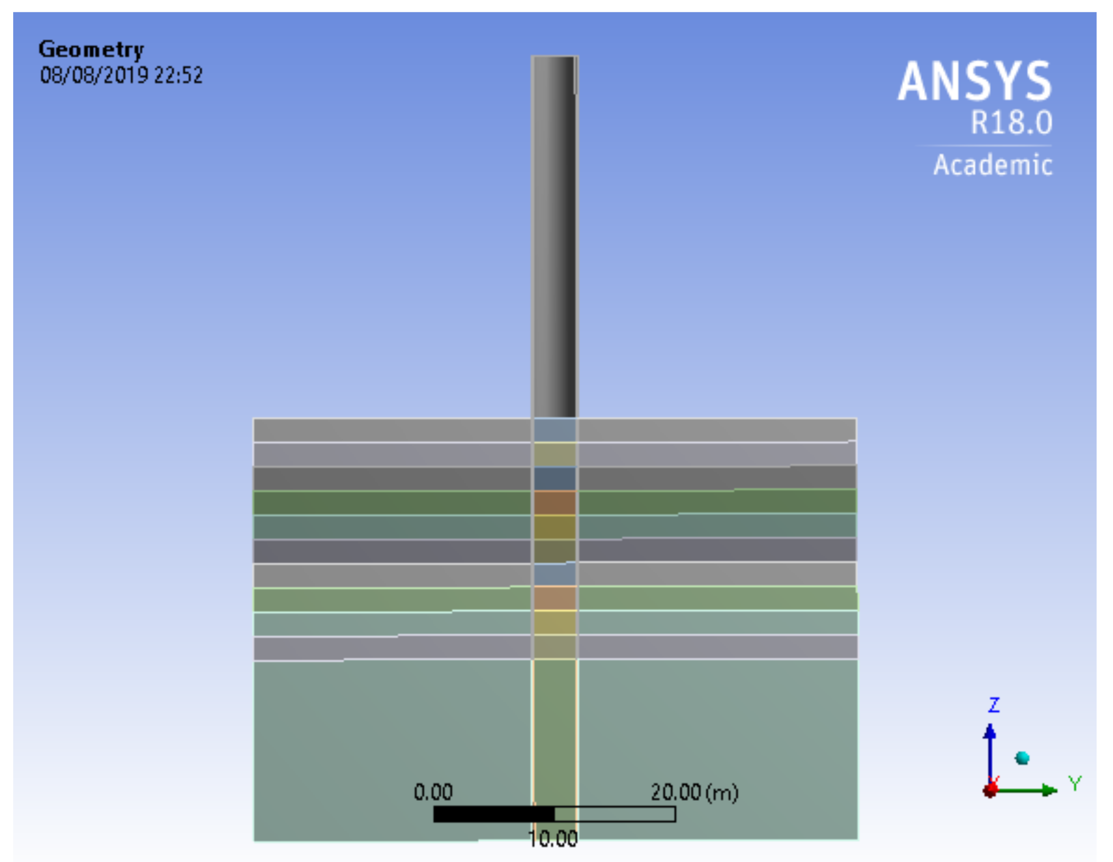
The numerical simulation of the cyclic behaviour of monopile requires a high computational effort, due to the size, non-linearity and complexity of the problem, as well as the need for time integration procedures to predict the evolution of the system performance in time. As both geometry and loads are symmetric, only half of the problem will be modelled. An example of a symmetric model is shown in Figure 2.
The model requires the symmetric boundary condition (symmetry with respect to the yz-plane) to be applied to both pile and soil elements, which means that any displacement in the x-direction for all nodes contained in the symmetry place will be prevented.
In this research, the overall sizes of the model are similar to those reported by [18]. The total horizontal extension of the model is equal to 12 D (where D is the diameter of the pile) and the overall depth of the soil is equal to 1.5 L (L denoting the length of the pile), as depicted in Figure 2. These sizes of the model are proven to generate very limited boundary effects.
2.2. Pile Modelling
The pile was modelled as a hollow solid element. It is assumed as linear, elastic steel, because it is much stiffer than the soil, and therefore high strains over its yielding limit are not expected to occur. The pile thickness can be calculated according to the equation given by the API offshore pile design guidelines of [12], according to which the pile diameter can be determined as:
where tp is the pile wall thickness (in mm), and D is the diameter of the pile (in mm).
The cyclic behaviour of the monopiles with D of 5 m, 6.25 m and 7.5 m have been modelled. The monopile geometrical properties used to study the cyclic behaviour are summarised in Table 1, and the properties of the steel used to investigate the cyclic behaviour of the monopile are those presented in Table 2.
2.3. Soil Modelling
The elasto-plastic Mohr-Coulomb constitutive model requires a very limited set of parameters, namely: friction angle, cohesion and dilation angle (in addition to the elastic properties of the soil to simulate its behaviour under the elastic range: Young’s modulus and Poisson’s ratio). All these parameters can be very easily determined in the laboratory, and therefore the uncertainty and the error when the Mohr-Coulomb model is used mainly comes from the limitation of the model itself rather than from the uncertainty in its calibration.
For saturated clay under undrained conditions, the Poisson’s ratio can be assumed as 0.5. However, to ease the convergence of the numerical simulation, it has been assumed as 0.495 in the present research. According to [19], the Young’s modulus of clay can be related to the undrained shear strength with a correlation factor Kc, which is a function of the over-consolidation ratio (OCR) and the plasticity index (PI) of clay, as shown in Figure 3.
For undrained clay behaviour, both friction and dilation angles are negligible. To avoid numerical instabilities, both angles are taken as small as 1 degree.
The cyclic behaviour of the monopiles in four different clayey profiles has been investigated. The first three profiles consist of clayey materials reported in [20] (clay type 1 to 3). The fourth profile analysed consists of layered clay, with two 10m deep layers of clay types 1 and 2. The properties of the four types of clay used to investigate the cyclic behaviour of monopile are summarized in Table 3.
2.4. Soil-Pile Interface
The soil-pile interface was modelled as frictional in this research. The frictional contact defined in Ansys® allows a gap to be formed between pile and soil, as illustrated in the example shown in Figure 4. The required input parameter for the frictional contact is the coefficient of friction. The research on pile-clay interface friction developed by [21] was used, in which the relationship between the plasticity index and the coefficient of friction is the one shown in Figure 5, where ultimate and peak represent the ultimate interface friction and peak interface friction angles, respectively. According to [22], peak corresponds to the behaviour of rigid monopiles. Therefore, tan peak curve shown in Figure 5 was used to determine the coefficient of friction in this research, through which for any given plasticity index, the corresponding coefficient of friction can be determined. The coefficients of friction for each model, obtained from Figure 5, are summarized in Table 4.
2.5. Input Loads
To reduce the computational effort, the superstructure of the offshore wind turbine above 30 m over the mudline was simplified as a vertical load, representing the weight of the superstructure and turbine. At this elevation, a punctual horizontal load, assumed as the resultant force of wind and sea waves, is also applied either statically or cyclically.
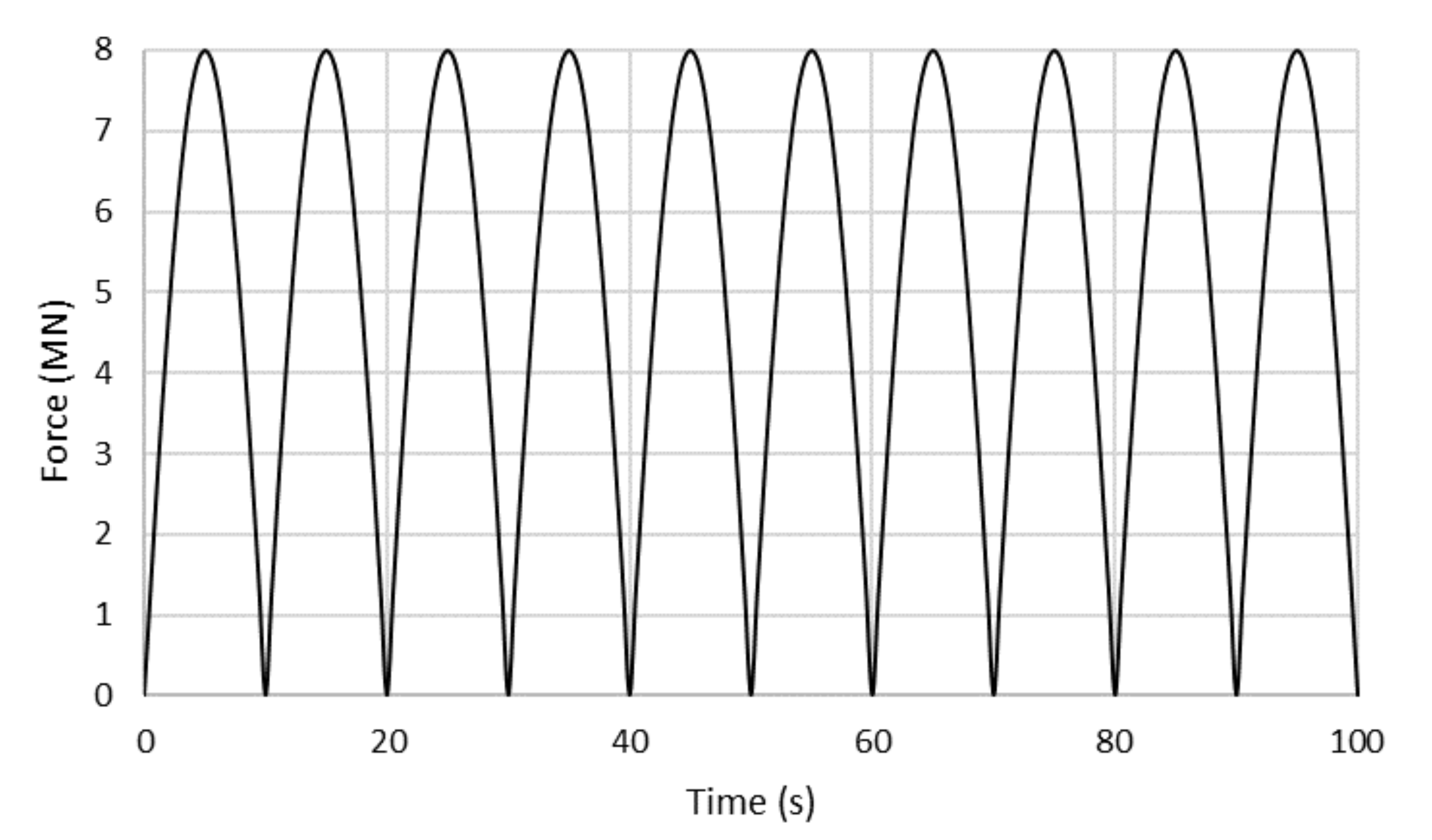
The typical resultant dynamic load that an offshore wind turbine monopile experiences is of one-way cyclic type, as reported by [18]. Therefore, as in that research, a one-way cyclic sinusoidal load was used in the present paper to represent the horizontal load applied to the monopile. A total of 100 cycles were applied to each model, and each cycle lasted 10 s (corresponding to a frequency of 0.1 Hz). From [23], the typical peak vertical and horizontal loads for a 3.5 MW offshore wind turbine are 6 MN and 4 MN, respectively. The peak load represent the combination of critical wave and maximal wind loads. However, the size of offshore wind turbines has significantly increased during recent years, and these sizes are expected to keep on increasing in the next future. Therefore, both vertical and horizontal loads may be doubled for a 5 MW offshore wind turbine, which has a size of about twice larger than those of a 3.5 MW one. Therefore, the peak vertical and horizontal loads applied on the models used to investigate the cyclic behaviour of monopile have been 12 MN and 8 MN, respectively. The horizontal load applied for the cyclic simulation can be described as:
where abs denotes absolute value (one-way load); Fmax denotes the amplitude of the horizontal load (8 MN in this scenario, for a 5 MW turbine); T represents the period of the load (10 s in this case), and t is the time. The loading diagram of the first 10 cycles is shown in Figure 6.
2.6. Mesh Density and Sensitivity Analysis
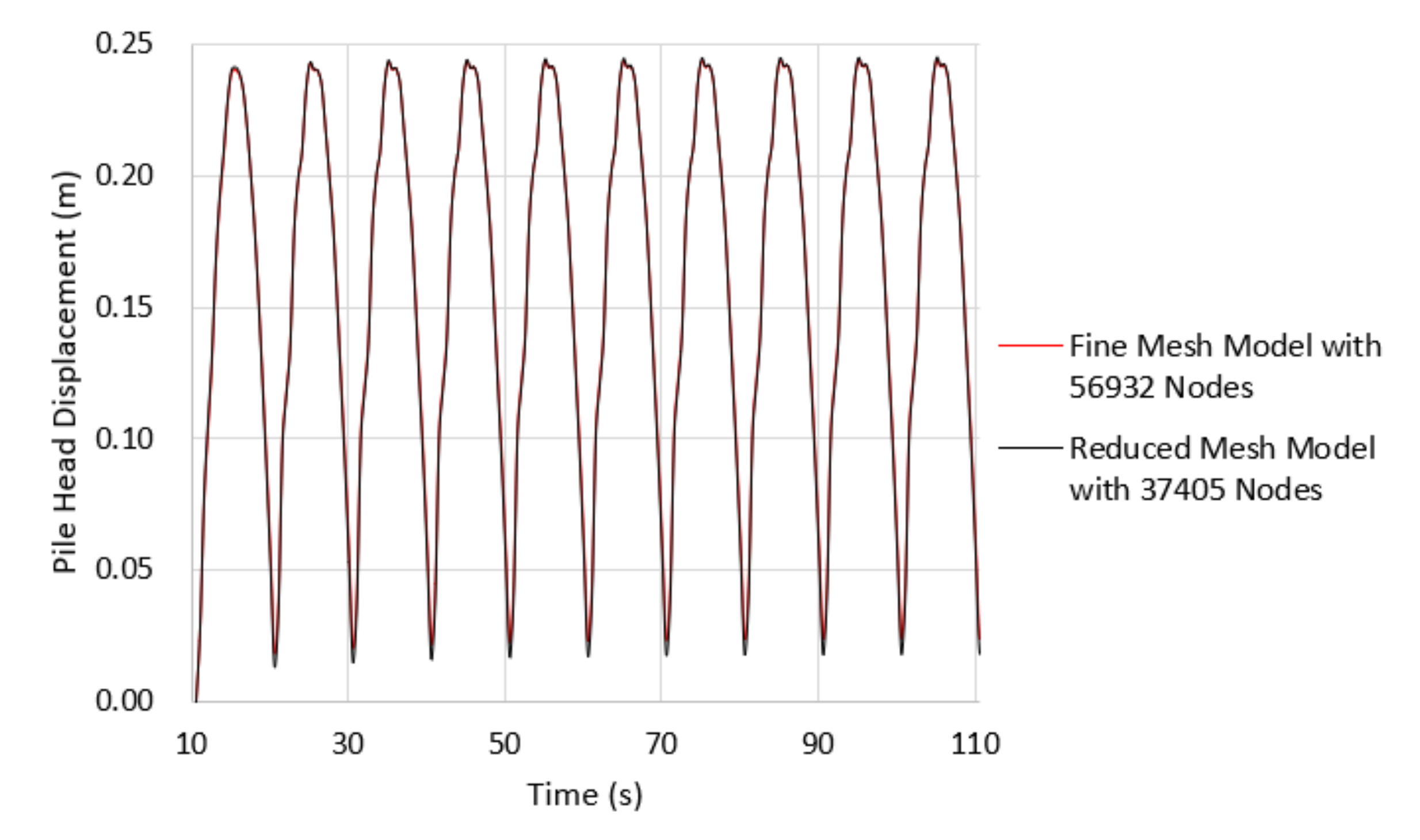
The computational effort is proportional to the mesh density. The coarser possible mesh density without compromising the accuracy is explored hereinafter. To capture the pile-soil interaction accurately, the mesh density in the soil domain must be higher in the proximity of the soil-pile interface. Since a negligible deformation close to the boundary of the model was found, the mesh density close to these locations was also coarser. Thus, the mesh density was reduced gradually from the interface to the edges. The reduced mesh density model resulted in a total of 37,405 nodes. [18] found that accurate results can be generated for the model with 50,622 nodes for an offshore wind turbine monopile foundation problem. To investigate the performance of the reduced mesh density model, a sensitivity analysis on the mesh density was carried out. A model with a fine mesh resulting in 56,932 nodes was running for 10 cycles and compared with the results achieved with the 37,405 nodes model. The mesh reduction in this analysis is merely applied in the vertical direction as shown in Figure 7 since the accuracy in the horizontal direction is the most important aspect of this research (because the input loads are horizontal) and cannot be compromised. Some loss of accuracy due to the mesh reduction in the vertical direction can be assumed though. Both meshes are shown in Figure 7.
The time history of the pile head displacement has been plotted in Figure 8, where it can be seen how the reduced mesh density model slightly over-estimates the pile head displacement. However, the results generated with the coarser model are close enough to those of the denser model, and therefore the accuracy of the solutions is not significantly compromised with it, while the efficiency highly increases. Therefore, the coarser mesh is employed in the simulations presented hereinafter.
3. Validation of the Numerical Model
3.1. Centrifuge Tests
Both monotonic and cyclic numerical models have been validated using the centrifuge tests results obtained by [16], who report results out of 1000 cycles of loading. Those tests were conducted on large diameter monopiles (dislike other cases on small diameter of rigid piles such as those carried out by [24,25], among others). In this section, these centrifuge tests are described and discussed.
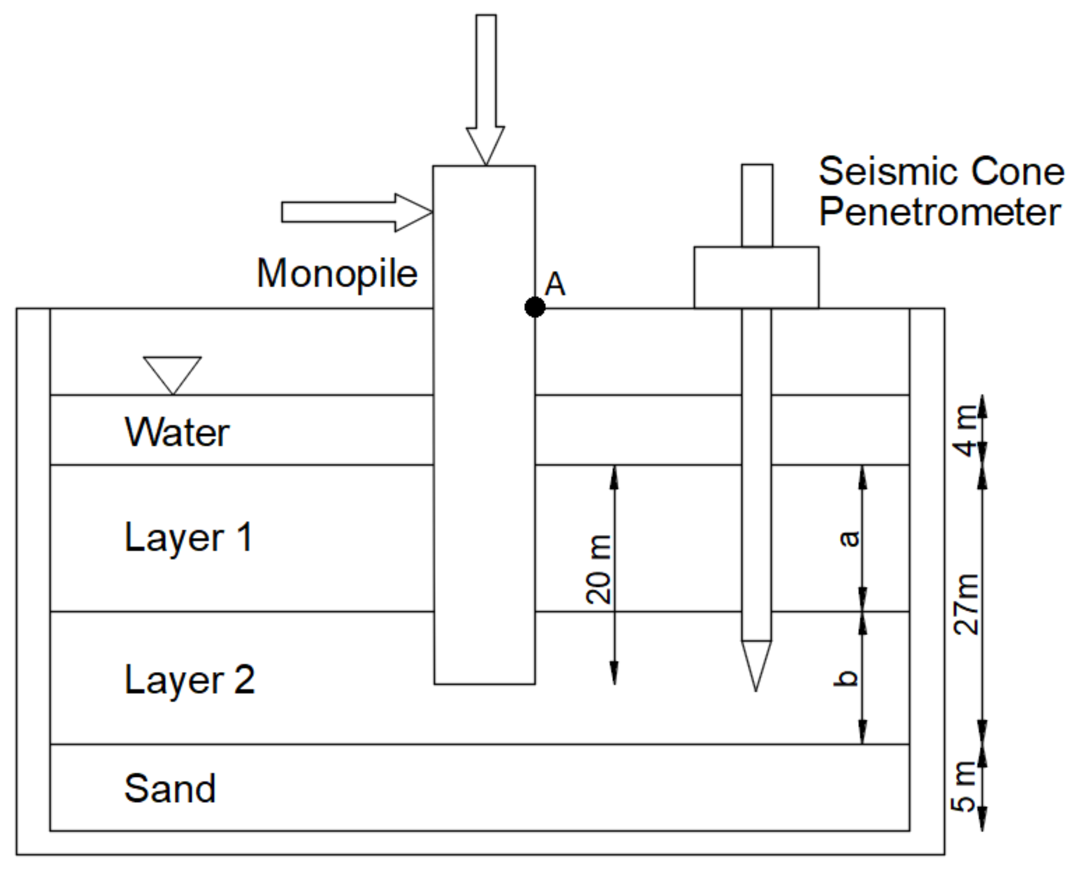
Ref. [16] investigated two pile geometries with pile diameters of 3.83 and 7.62 m in five different soil profiles. A total of nine centrifuge tests were carried, namely test numbers OWF-01 to OWF-09. Figure 9 shows the setup for the centrifuge tests. The embedded length of the pile was 20 m, and the force was applied 30 m above the mudline. The vertical force applied was 6MN for the 3.83 m diameter pile and 12 MN for the 7.62 m diameter pile. Table 5 summarises the five different site conditions, while Table 6 shows the summary of these nine tests.
Tests OWF-01 to OWF-03 (Phase I) were monotonic experiments with 3.83 m diameter piles on the prototype scale. Moreover, tests OWF-04 to OWF-08 (Phase II) were cyclic analyses with 3.83 m diameter piles on the prototype scale. Test OWF-09 (Phase III) was a cyclic test with a 7.62 m diameter pile on the prototype scale.
The cyclic tests (OWF-04 to OWF-09) were subdivided into seven stages based on their loading patterns, as shown in Table 7 [16]. In general, the tests in stages 1, 2 and 5 were subjected to one-way cyclic loading. The tests in stage 7 were subjected to monotonic push. Either 1-way or 1.25-way cyclic loading is applied in the rest of the stages. From stages 1 to 6, the test with a higher stage number has a larger peak load.
Tests OWF-03 and OWF-09-stage-4 have been selected in the present paper to validate monotonic and cyclic numerical models, respectively. The rationale behind this selection was to choose the centrifuge tests with potentially lowest uncertainty within their categories (i.e., monotonic and cyclic). The experiment results obtained for OWF-03 may have lower uncertainty than the other two monotonic tests (i.e., OWF-01 and OWF-02) because it was the last monotonic test conducted, which means that the experiment operator [16] has developed sufficient experience and skills from the previous runs OWF-01 and OWF-02. Therefore, OWF-03 is selected for the validation of the monotonic numerical model.
As previously described, the cyclic tests reported by [16] are subdivided into several stages based on the loading profiles. The initial aim of that research was to conduct 1-way and 1.6-way cyclic loading rather than 1-way and 1.25-way because the monopile has the highest response (accumulated rotation) under 1.6-way load. However, this plan was abandoned because of the unaccepted experiment error [16], implying that the monopiles which had higher responses during the experiments may also have more uncertainty in their solutions. On the contrary, those monopiles which experienced an extremely low response may be associated with considerable uncertainty as well. For example, the experiment results from Stage 1 have not been documented by [16], possibly because the peak loads in stage 1 (3 and 6 kN) were not high enough to develop the non-linear soil behaviour. Although the results are documented for stage 2, the highly dispersed data points shown in this stage seem to indicate high uncertainties. Therefore, the tests subjected to moderate peak loads seem more reliable. Those tests are on stages 3 and 4. One source of uncertainty given by loads application during the experiments can be quantified by exploring Table 7, where the ideal minimum load should be zero for the 1-way scenario and 0.25 times its maximum load, for the 1.25-way scenario. Therefore, the uncertainty can be simply calculated by the difference between actual and ideal minimum loads divided by the peak load. From Table 7 and the application of the proposed uncertainty calculations, OWF-06-stage-4 and OWF-07-stage-4 have the lowest uncertainty, which is 0% and 1%, respectively. Furthermore, [16] disclosed that OWF-06 and OWF-09 might have larger uncertainties because of reported inappropriate operations. Therefore, the OWF-07-stage-4 is adopted as the one with the lowest uncertainty in these cyclic tests.
The material used in the test was Kaolin, and the triaxial test conducted for this clayey material, along with its main soil properties (such as specificity gravity and plasticity index), are documented by [16]. Besides the triaxial test, the over-consolidation ratio and the undrained shear strength profile along with the depth were measured during the tests.
3.2. Input Parameters and Results of the Validations
To closely represent the real soil conditions during the tests, the soil profile was sub-divided into 11 layers in the model as shown in Figure 10. The top 20 m of soil where the pile was embedded were divided into 10 layers, 2 m deep for each one of them. The soil beneath the pile was modelled as a single layer since no significant soil-pile interaction was expected at this location.
The soil properties reported by [16] (plasticity index, the over-consolidation ratio and the undrained shear strength profile along with the depth) are employed in the numerical simulations. The Kaolin clay employed in these tests had a plasticity index equal to 33%. As both the plasticity index and the OCR are known, the correction factor Kc for each layer can be obtained from Figure 3. Therefore, the Young’s modulus (Es) for each layer can be calculated by the correction factor (Kc) multiplied by the undrained shear strength (Cu) in each layer. The input soil properties for each layer are presented in Table 8. According to [16], centrifuge tests OWF-03 (used for validating the monotonic behaviour) and OWF-07-stage-4 (used for validating the cyclic behaviour) were conducted using different soils, the properties of which are summarized in Table 8. Layer 1 is the surface soil layer, while layer 11 is the bottom one.
The pile geometry and the applied loads were exactly the same as for the prototype scale in the centrifuge test: D = 3.83 m, tp = 1.67 mm and L = 20 m. The coefficient of friction between pile and soil can be obtained from Figure 5, taken as 0.250 for the 33% plasticity index.
According to the centrifuge test conducted by [16], the monotonic pushover was displacement-controlled. The reaction force at the pile head and the mudline displacement were measured during the centrifuge test [16]. The mudline displacement was measured at point A as shown in Figure 9. Figure 11 shows the validation for the monotonic model. Despite some instability observed in the experimental results, probably due to inaccuracy of the transducers, it can be seen that the agreement between numerical and experimental results is excellent. From this analysis, it can be concluded that the Mohr-Coulomb constitutive model is reliable enough to describe the monotonic behaviour of monopiles in clay. From the figure, it can also be seen that the numerical simulation slightly over-estimates the initial horizontal displacement which is consistent with previous results, reported by [10,14].
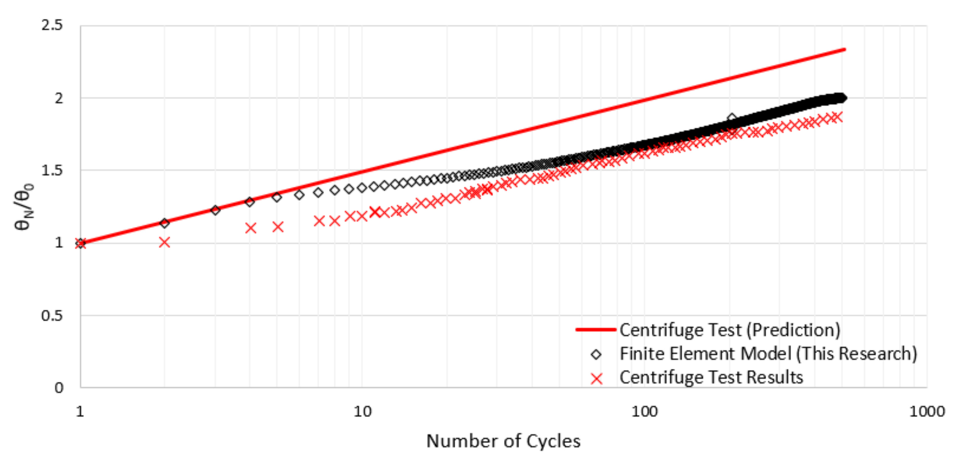
Ref. [16] documented the cyclic behaviour of the monopiles as the cumulative rotation for the pile at the mudline. Same as [11,16], in this paper the cumulative rotation for each cycle has been normalized with respect to the rotation of the first cycle. The results obtained from this centrifuge test are presented in Figure 12. Moreover, Ref. [16] reported a comparison between their experimental results and a prediction with the methodology proposed by [11], also plotted in Figure 12. The results obtained with the numerical model developed in the present research are also included in Figure 12, showing a much better agreement when compared with the experimental results. From this comparison, it can be concluded that the Mohr-Coulomb constitutive model can be considered accurate enough to describe the pseudo cyclic behaviour (cumulative rate of rotation) of monopiles in clay. It should be noticed that only the cumulative rate of rotation (N/0) can be validated; the force-displacement hysteresis loops cannot be validated by the centrifuge test due to the well-known limitation of Mohr-Coulomb constitutive model. This is the reason it is called pseudo cyclic behaviour (i.e., the cumulative rate of rotation is true, but the force-displacement hysteresis is pseudo). Therefore, the following analyses, based on Mohr-Coulomb model, are merely focused on the pile rotation in the first cycle (monotonic behaviour) and its cumulative rate of rotation.
4. Results
Once both monotonic and cyclic models have been validated, a set of simulations has been conducted to investigate the cyclic behaviour of monopiles with different geometries and types of clay. Three piles, with a diameters, D, of 5, 6.25 and 7.5 m, have been modelled, using three types of clay with undrained shear strength, Cu, of 50, 75 and 100 kPa. One dual-layered clay was studied, with a top layer of 50 kPa over another layer of 75 kPa. The embedded length of the pile, L, ranges from 25 to 30 m (with intervals of 1 m) in the case of Cu = 50 kPa. All the conducted simulations are summarised in Table 9. The detailed input parameters of the models can be seen in the Methodology section.
4.1. Time History of the Pile Rotation
The pile rotation angle can be calculated as follows:
where is the pile rotation (in degrees), represents the horizontal pile head displacement of the head of the pile (obtained from the model), and H is the total pile length. The rotation point of the studied monopiles in clay was found at about 75% of the embedded depth; this is also consistent with previous research [20].
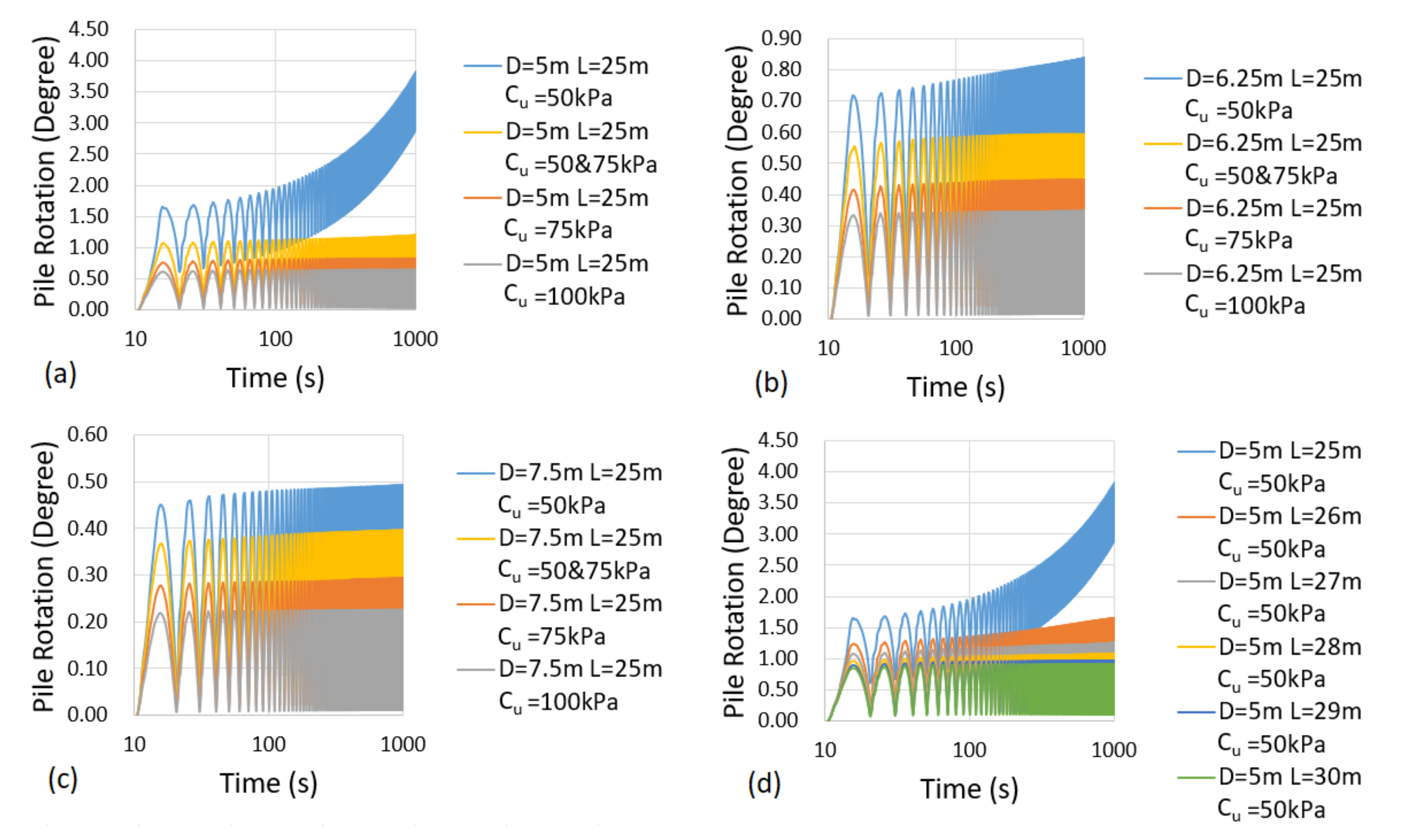
The time histories of the pile rotation for the 17 simulations are plotted in Figure 13. Figure 13a shows this result for the 5 m diameter pile at 25 m of embedded depth in various types of clay. As expected, the pile rotation in softer clays (with lower values of Cu) is larger than for stiffer clays (larger Cu). From Figure 13a–c, the dual-layered soil with 50 kPa (on the top layer) and 75 kPa (at the bottom layer) of undrained shear strength has an intermediate pile rotation compared with the pile rotation in the 50 kPa and 75 kPa soils. The same trend was also found for the 6.25 and 7.5 m diameter piles, which are shown in Figure 13b,c, respectively.
From Figure 13a–c, we can conclude that the pile rotation decreases as the pile diameter increases. Furthermore, it has been found that the 5 m diameter pile embedded in 50 kPa clay with 25 m of embedded depth yields unstable behaviour because the rotations do not reach stable values, as in the other cases. From Figure 13d, after the embedded depth increases from 25 to 26 m, the stability of the pile significantly improved. The pile rotation decreased when the embedded depth of the pile increased. Therefore, the increment of pile diameter and embedded depth can reduce the pile rotation and the stability of the pile can also be improved.
It is clear that unstable behaviour happened in the 5 m diameter pile embedded in 50 kPa clay with 25 m of embedded depth. However, the monopile can also fail due to the accumulated rotation reaching a certain value after experiencing a high number of cycles, in the range of millions. This is away from the computation ability of the numerical simulation such as the one presented in this paper. Therefore a procedure is required to predict the monopile rotation after any number of cycles. This procedure is derived and discussed in the following sections.
4.2. Pile Rotation in the First Cycle
The pile rotations in the first cycle for the 17 simulations were extracted and summarized in Table 10. The accuracy of the pile rotations in the first cycle is mainly related to the monotonic performance of the numerical model, validated in many research studies as well as in the current one. Therefore the accuracy of the pile rotations in the first cycle generated in this research can be assumed to be significantly high.
As discussed in the previous sections, the pile rotation is related to the pile diameter, embedded depth and undrained shear strength of the soil. Reducing the pile diameter and embedded depth results in increasing the pile rotation. The dual-layered soil with 50 kPa and 75 kPa of undrained shear strength has an intermediate pile rotation compared with those reached with the 50 kPa and 75 kPa soils. The average undrained shear strength (i.e., 62.5 kPa) can be taken to represent the behaviour of the dual-layered soil. A significant linear relationship was found between the pile rotation in the first cycle in the logarithm scale and D × L × ln(Cu) in the natural logarithm scale (where D and L are given in meters and Cu in kPa). This relationship can be described using the following expression:
where 0 represents the rotation in the first cycle (in degrees), and exp denotes exponential.
In Figure 14, the value of D × L × ln(Cu) is plotted against the corresponding pile rotation in the first cycle for each simulation. This figure shows a strong correlation between both amounts, as previously mentioned, demonstrating a low uncertainty when Equation (4) is employed to predict the pile rotation in the first cycle.
In addition to the simulations conducted with horizontal load with amplitude of 8 MN, further analysis with 4 MN and 2 MN have also been conducted. The maximum pile rotations in the first cyclic for these amplitudes are also presented in Figure 14, from which it can be concluded that these correlations are parallel one to each other in the range of D × L × ln(Cu) values explored. Initial rotations for other amplitudes (out of 8 MN) can be obtained by interpolation, from the values presented in Figure 14. The regressions shown in Figure 14 can be generalised as:
Since the regressions are roughly parallel one to each other, the constant b can be conservatively taken as 0.004. The constant a follows can be expressed as:
where F is the peak horizontal load (in MN).
4.3. Cumulative Rate of Rotation
From the previous section, Equation (5) was developed to predict the initial pile rotation for the monopile with any given pile geometry embedded in clay with any undrained shear strength. The pile rotation in any given number of cycles can be correlated to the initial rotation, as justified hereinafter.
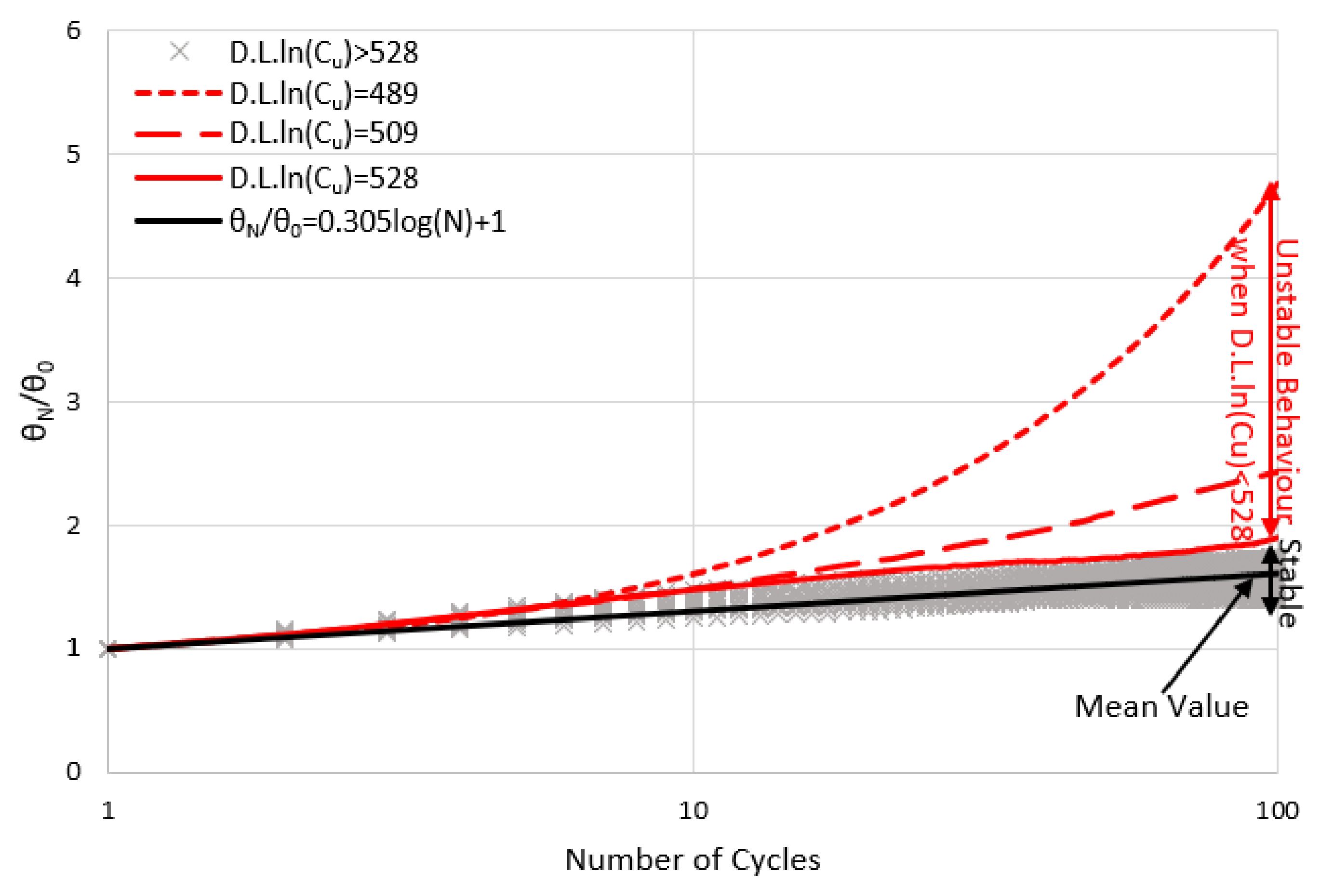
The cumulative rate of rotation is the ratio between the rotation in each cycle N, (N), and the rotation in the first cycle (0). The cumulative rate of rotation for each simulation has been plotted in Figure 15, from which we can see that, in most of the simulations, it follows a linear trend, in the logarithm scale, with the number of cycles, which is consistent with the findings given by other authors [11,16]. This indicates that the speed of the cumulative rate becomes lower as the number of cycles increases. However, the tendency is significantly different in the case of a 5 m diameter monopile embedded in 50 kPa clay, with L = 25 m (D × L × ln(Cu) = 489), 26 m (D × L × ln(Cu) = 509) and 27 m (D × L × ln(Cu) = 528). This indicates that instability happens in these cases (i.e., when D × L × ln(Cu) < 528). For these unstable monopiles, the pile diameter or the embedded depth should be increased to reduce the pile rotation.
The findings from the previous section can also be used to determine the stability of the monopile. The monopile behaviour becomes unstable when D × L × ln(Cu) is smaller than 528. Therefore, the stability can be immediately determined once the pile geometry and clay properties are available.
As in Figure 15, the cumulative rate for each simulation is very similar when the monopile reaches a point of stable behaviour (i.e., D × L × ln(Cu) > 528). Therefore, the mean of the cumulative rate can be used to represent stable monopile cyclic behaviour. The mean of the cumulative rate can be described as:
For the case of 8 MN of amplitude of loading (i.e., 5 MW wind turbine), inserting Equation (4) into Equation (7) and rearranging, We can have:
Using Equation (8), the monopile rotation of a 5 MW wind turbine in any load cycle can be determined.
When D × L × ln(Cu) < 528, Equations (7) and (8) cannot be used, and the corresponding numerical simulation should always be conducted in such cases to determine the cumulative rate.
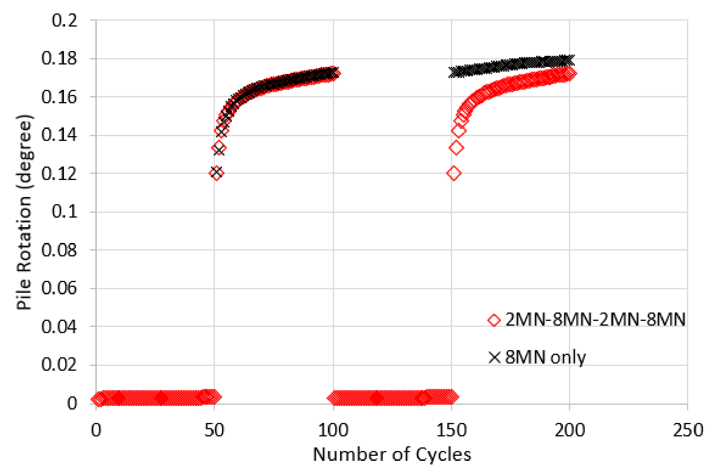
To conclude this section, the response of a monopile foundation under variable amplitudes of harmonic loading have been analysed. The geometry of this model is exactly same as the model with 7.5 m diameter embedded 25 m in 50 kPa undrained shear strength of clay. The horizontal load applied can be described as
A total of 200 cycles were applied to this model, with each cycle lasting 10 s (0.1 Hz). As it can be seen in Equation (9), the amplitude for the first 50 cycles was 2 MN, 8 MN for the next 50 cycles, 2 MN for the following 50 and again 8 MN for the last 50 cycles. The evolution of the rotation of the pile in time during this simulation is presented in Figure 16, in comparison with the rotation obtained during 100 cycles of a constant amplitude of 8 MN, plotted in two parts, jointly with the results for the two 50 stages (of 50 cycles each) of 8 MN for the multi-amplitude loading. From this figure, it can be concluded that the rotation predicted in the case of load with variable amplitude is almost identical to the one achieved only for the number of cycles with higher amplitude (100 cycles of 8 MN). Therefore, it can be concluded that in clayey soils, the effect of low amplitudes of loading is erased by higher loads. This is extremely relevant to save computational efforts in the simulations, as demonstrates that the loads with higher amplitudes (such as those during storms) are those controlling the pile rotation, and the lower loads can therefore be neglected.
Therefore, Equations (7) and (8) can be considered accurate enough, just applying the peak expected amplitude of load and the corresponding expected number of cycles for that amplitude.
5. Procedure to Design Monopiles in Clay
To improve the design procedures for offshore wind turbine monopile foundations in clay, a new procedure is presented in this paper, based on the previous findings. This new methodology can be described as follows:
- 1.
- determine the capacity of the offshore wind turbine; estimate the corresponding design horizontal load;
- 2.
- measure the undrained shear strength (Cu) of the clay in the seabed;
- 3.
- estimate the initial pile geometry that included the pile diameter (D) and the embedded depth (L);
- 4.
- calculate the pile wall thickness (through Equation (1));
- 5.
- 6.
- estimate the number of storm cycles that the offshore wind turbine may experience;
- 7.
- calculate the pile rotation under the number of storm cycles using Equation (7);
- 8.
- if the rotation was larger than the design requirement, then we need to modify the dimensions of the pile and repeat the procedure from step 3.
It should be noticed that this design method was derived from the simulation results. The numerical simulations conduced in this research covered a monopile diameter range from 5 m to 7.5 m and undrained shear strength values for clays ranging between 50 and 100 kPa. Therefore, this design method is reliable for sizes and undrained shear strength within those ranges. For other values, the prediction may be unreliable. As previously discussed, the cyclic loads with higher amplitudes will erase the effect of those cycles with lower amplitudes. Hence, to design monopiles in clays, only the cycles under extreme loading conditions (i.e., storm events) that the offshore wind turbine will ever experience, have to be considered and explored. Equation (7) was derived based on the simulations undertaken for 8 MN peak horizontal cyclic loads, representing a 5 MW offshore wind turbine. To design other types of wind turbine foundations with lower capacity (e.g., 3.5 MW offshore wind turbine), Equation (7) is still conservative since a lower amplitude was investigated to have lower cumulative rate of rotation.
For a horizontal load of 8 MN, if D × L × ln(Cu) is smaller than 528, then the monopile may have unstable behaviour. In such a case, it is recommended to conduct an accurate numerical simulation to predict the rotation. Conservatively, the pile diameter (D) or the embedded depth (H) can be increased and repeated as in step 3.
5.1. Design Example
5.1.1. 5MW Offshore Wind Turbine
In this example, the clay in the seabed is assumed to have 92 kPa of undrained shear strength. The monopile employed to support 5 MW offshore wind turbine was designed to have a diameter of 7 m and 30 m of embedded depth. The offshore wind turbine was predicted to experience 10 thousand large storms, each one with 100 cycles of horizontal loads with 8 MN of amplitude of harmonic, one-way load. We first check if the pile behaviour will be in the stability range:
Therefore, the monopile is stable. The number of storm cycles is estimated as 106, and therefore, the pile rotation can be calculated as
Thus, the expected maximum pile rotation after 1 million cycles of extreme horizontal loads is 0.32 degree for a 7 m diameter monopile embedded 30 m in 92 kPa clay.
5.1.2. 3.5 MW Offshore Wind Turbine
In this case, the seabed soil is assumed to be the same as in the previous case, with 92 kPa of undrained shear strength. The monopile used to support 3.5 MW offshore wind turbine was designed to have a diameter of 5 m and 30 m of embedded depth. The weather conditions are also the same, with 106 of storm cycles, this time with 4 MN of amplitude of horizontal load, as the turbine is smaller. From the regression equation shown in Figure 14, for 4 MN peak horizontal load the maximum rotation in the first cycle can be calculated as
We can assume Equation (7) is conservative to estimate the cumulative rate of rotation for 3.5 MW offshore wind turbine monopile foundation. Therefore
Therefore, the expected maximum pile rotation after 1 million cycles of extreme horizontal loads is 0.49 degree for a 5 m diameter monopile embedded in 92 kPa clay with 30 m of embedded depth.
6. Conclusions
Monopiles can nowadays be considered to be the most economic and reliable solution for offshore wind turbine foundations. In the current design guidelines, p-y curves are derived for small diameter piles, as those used for gas platform foundations. Applying the current design guidelines to offshore wind turbine monopile foundations might generate an uneconomic solution.
In this research, the Mohr-Coulomb model was used to represent the undrained behaviour of clay. Frictional contact was considered to describe the soil-pile interface. Both monotonic and cyclic performances of the numerical model developed in this research were successfully validated with reported centrifuge tests, demonstrating the reliability of the adopted assumptions. The successful validations benefited from the low uncertainty in the calibration of the Mohr-Coulomb model. For the undrained scenario, only the undrained shear strength and the over-consolidation ratio need to be measured during the experiments.
After the validation, a set of numerical models were conducted to investigate the cyclic behaviour of monopiles with various geometries and different types of clay. The time history of the pile rotation, for each simulation, was extracted and analysed. The monopile rotation in clay is related to the pile diameter, the embedded depth and the undrained shear strength of clay. After analysing the data, an empirical expression to obtain the rotation for the first cycle of loading was obtained. To predict the pile rotation at any cycle, the cumulative rate of rotation was determined. Similar cumulative rates were found for monopiles displaying stable behaviour for increasing number of cycles. However, for unstable monopiles, the cumulative rate was significantly larger than the prediction. For the range of geometries and undrained shear strengths simulated, the monopiles were found to be stable if D × L × ln(Cu) is larger than 528.
Finally, a new design procedure for offshore wind turbine monopile foundations in clay has been presented. For any monopile diameter range from 5 m to 7.5 m and undrained shear strength of clay range from 50 to 100 kPa, the maximum pile rotation in any cycle can be calculated using this procedure. Similar analyses can be conducted for other geometries and clayey materials, to generalise the procedure presented in this paper.
Author Contributions
Conceptualization and methodology, M.X. and S.L.-Q.; numerical models, M.X.; writing—original draft preparation, M.X.; writing—review and editing, S.L.-Q.; data analyses and visualization, M.X.; supervision, S.L.-Q. All authors have read and agreed to the published version of the manuscript.
Funding
This research received no external funding.
Institutional Review Board Statement
Not applicable.
Informed Consent Statement
Not applicable.
Data Availability Statement
Not applicable.
Conflicts of Interest
The authors declare no conflict of interest.
References
- HM Government. Meeting the Energy Challenge: A White Paper on Energy May 2007; Department of Trade and Industry: Norwich, UK, 2007; p. 7.
- European Commission. The Paris Protocol—A Blueprint for Tackling Change beyond 2020; European Union: Paris, France, 2015. [Google Scholar]
- European Union. The European Council in 2014; Publications Office of the European Union: Luxembourg, 2015. [Google Scholar]
- Ffrench, R.; Bonnett, D.; Sandon, J. Wind power: A major opportunity for the UK. Proc. Inst. Civ. Eng.—Civ. Eng. 2005, 158, 20–27. [Google Scholar] [CrossRef]
- Carter, J.M.F. North Hoyle offshore wind farm: Design and build. Proc. Inst. Civ. Eng.—Energy 2007, 160, 21–29. [Google Scholar] [CrossRef]
- Abdel-Rahman, K.; Achmus, M. Finite element modelling of horizontally loaded monopile foundations for offshore wind energy converters in Germany. In Proceedings of the International Symposium on Frontiers in Offshore Geotechnics (ISFOG), Perth, Australia, 19–21 September 2005. [Google Scholar]
- Moulas, D.; Shafiee, M.; Mehmanparast, A. Damage analysis of ship collisions with offshore wind turbine foundations. Ocean Eng. 2017, 143, 149–162. [Google Scholar] [CrossRef]
- DNV. Design of Offshore Wind Turbine Structures; Det Norske Veritas: Høvik, Norway, 2014. [Google Scholar]
- Doherty, P.; Gavin, K.; Casey, B. The geotechnical challenges facing the offshore wind sector. In Geo-Frontiers 2011: Advances in Geotechnical Engineering; Han, J., Alzamora, D.E., Eds.; American Society of Civil Engineers: Reston, VA, USA, 2011. [Google Scholar]
- Haiderali, A.; Nakashima, M.; Madabhushi, S. Cyclic lateral loading of monopiles for offshore wind turbines. In Frontiers in Offshore Geotechnics III, 1st ed.; Meyer, V., Ed.; CRC Press: Oslo, Norway, 2015; pp. 711–716. [Google Scholar]
- LeBlanc, C.; Houlsby, G.T.; Byrne, B.W. Response of stiff piles in sand to long term cyclic lateral loading. Geotechnique 2010, 60, 79–90. [Google Scholar] [CrossRef]
- API. Geotechnical and Foundation Design Considerations; American Petroleum Institute: Washington, DC, USA, 2011. [Google Scholar]
- LeBlanc, C. Design of Offshore Wind Turbine Support Structures: Selected Topics in the Field of Geotechnical Engineering. Ph.D. Thesis, Aalborg University, Aalborg, Denmark, 2009. [Google Scholar]
- Jung, S.; Kim, S.R.; Patil, A.; Hung, L.C. Effect of monopile foundation modeling on the structural response of a 5 MW offshore wind turbine tower. Ocean Eng. 2015, 109, 479–488. [Google Scholar] [CrossRef] [Green Version]
- Thomas, S. Geotechnical Investigation of UK Test Sites for the Foundations of Offshore Structures; The Stationery Office Books: London, UK, 1990. [Google Scholar]
- Lau, B.H. Cyclic Behaviour of Monopile Foundations for Offshore Wind Farms. Ph.D. Thesis, University of Cambridge, Cambridge, UK, 2015. [Google Scholar]
- ANSYS, Inc. Ansys® Workbench, Release 18.0 Academic; ANSYS, Inc.: Canonsburg, PA, USA, 2016. [Google Scholar]
- Lopez-Querol, S.; Cui, L.; Bhattacharya, S. Numerical methods for SSI analysis of offshore wind turbine foundations. In Wind Energy Engineering, 1st ed.; Letcher, T.M., Ed.; Academic Press: Cambridge, MA, USA, 2017; pp. 275–297. [Google Scholar]
- USACE. Engineering and Design-Settlement Analysis; U.S. Army Corps of Engineers: Washington, DC, USA, 1998.
- Haiderali, A.; Madabhushi, G. Three-dimensional finite element modelling of monopiles for offshore wind turbines. In Proceedings of the 2012 World Congress on Advances in Civil, Environmental, and Materials Research (ACEM 2012), Seoul, Korea, 26–29 August 2012; KAIST: Seoul, Korea, 2012. [Google Scholar]
- Lehane, B.M.; Chow, F.C.; McCabe, B.A.; Jardine, R.J. Relationships between shaft capacity of driven piles and CPT end resistance. Proc. Inst. Civ. Eng.—Geotech. Eng. 2000, 143, 93–101. [Google Scholar] [CrossRef]
- Ramsey, N.; Jardine, R.; Lehane, B.; Ridley, A. A review of soil steel interface testing with the ring shear apparatus. In Offshore Site Investigation and Foundation Behaviour; Society for Underwater Technology: London, UK, 1998. [Google Scholar]
- Byrne, B.W.; Houlsby, G.T. Foundations for offshore wind turbines. Philos. Trans. R. Soc. A 2003, 361, 2909–2930. [Google Scholar] [CrossRef] [PubMed]
- Zhang, C.; White, D.; Randolph, M. Centrifuge modeling of the cyclic lateral response of a rigid pile in soft clay. J. Geotech. Geoenviron. Eng. 2010, 137, 717–729. [Google Scholar] [CrossRef]
- Hong, Y.; He, B.; Wang, L.Z.; Wang, Z.; Ng, C.W.W.; Masin, D. Cyclic lateral response and failure mechanisms of semi rigid pile in soft clay: Centrifuge tests and numerical modelling. Can. Geotech. J. 2017, 54, 806–824. [Google Scholar] [CrossRef]
Figure 1.
The major types of offshore wind turbine foundation (after [7]).
Figure 1.
The major types of offshore wind turbine foundation (after [7]).
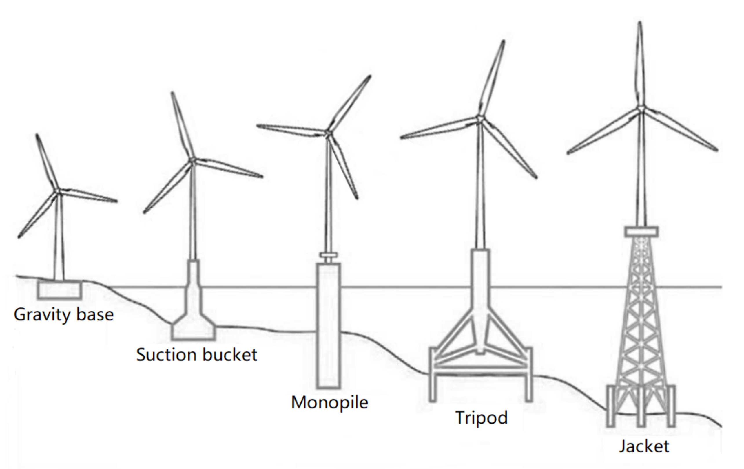
Figure 2.
Symmetric model used in this research and its overall dimensions.
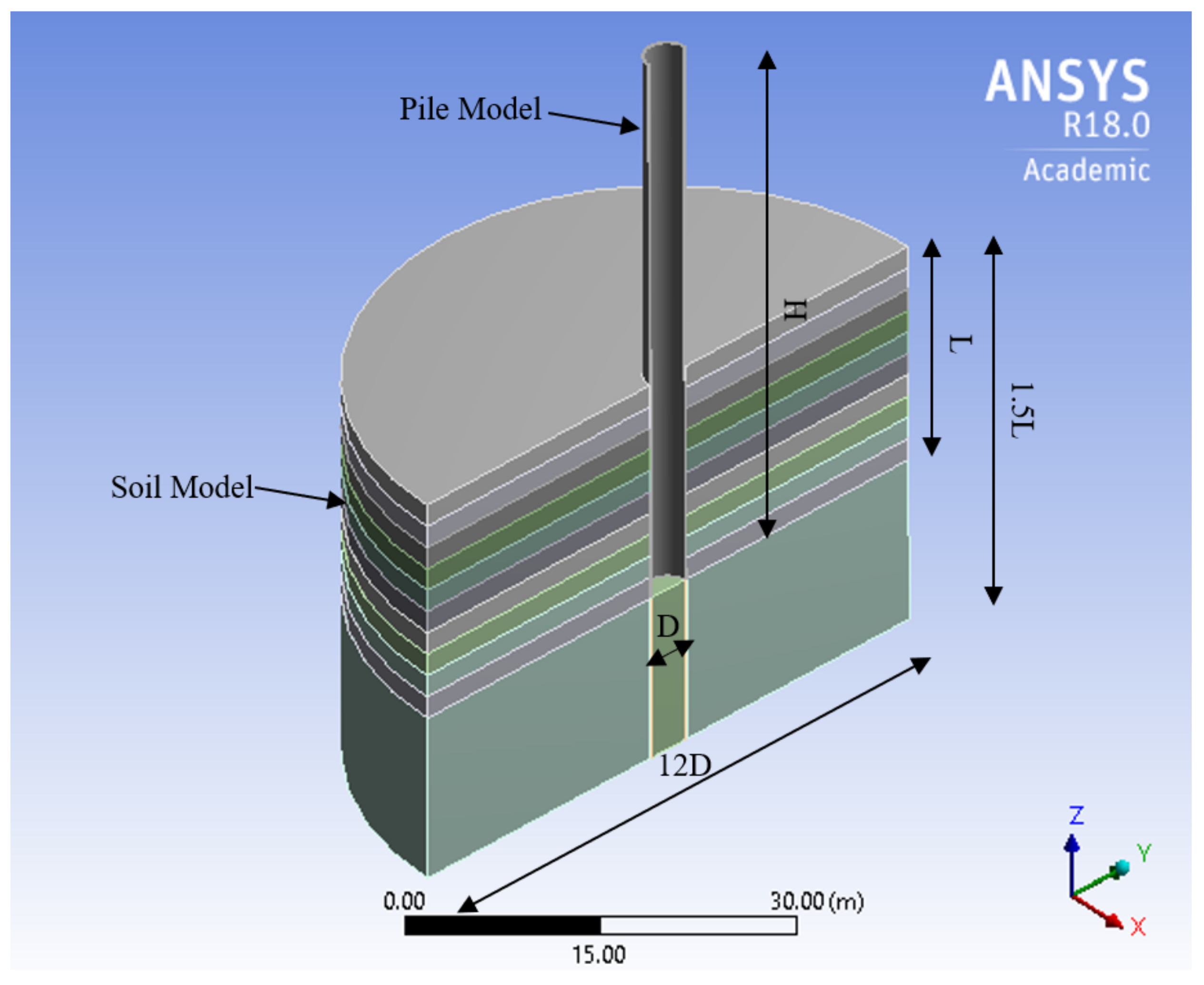
Figure 3.
The relationship between Kc and the over-consolidation ratio (OCR) (after [19]).
Figure 3.
The relationship between Kc and the over-consolidation ratio (OCR) (after [19]).
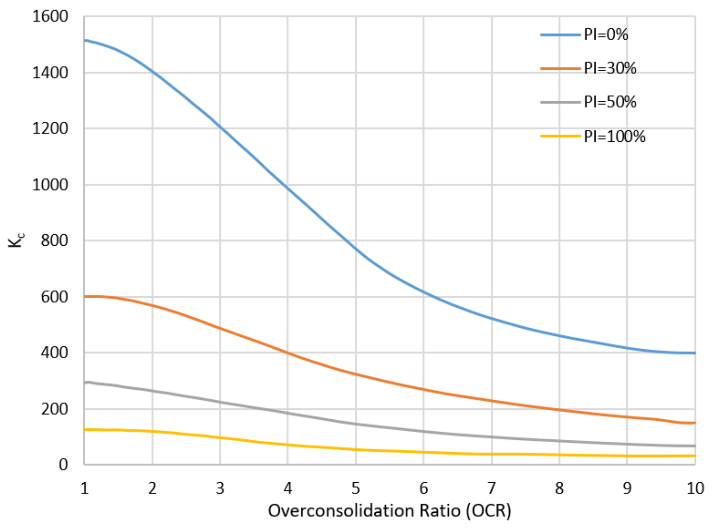
Figure 4.
Illustration of the formed gap between pile and soil during analysis of lateral load.
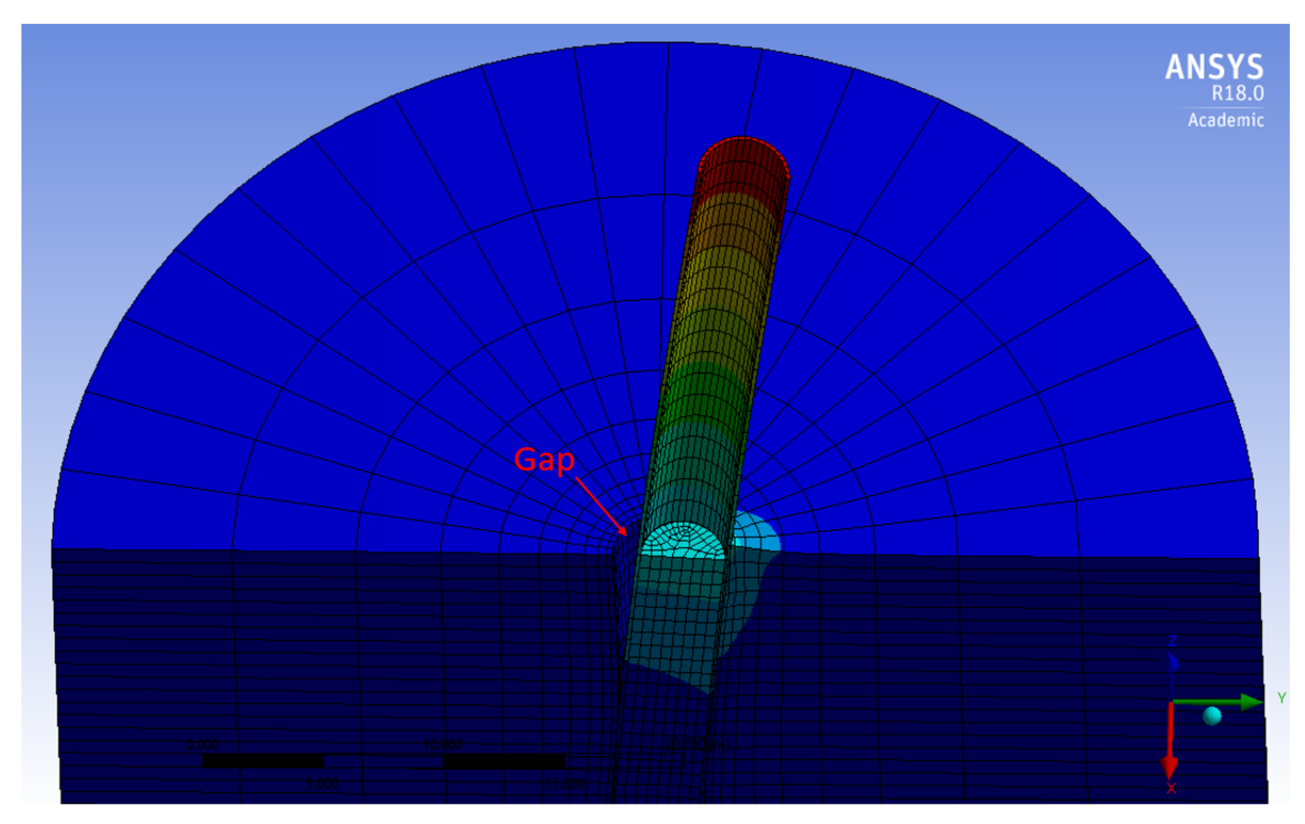
Figure 5.
The relationship between the plasticity index and the coefficient of friction (after [21]).
Figure 5.
The relationship between the plasticity index and the coefficient of friction (after [21]).
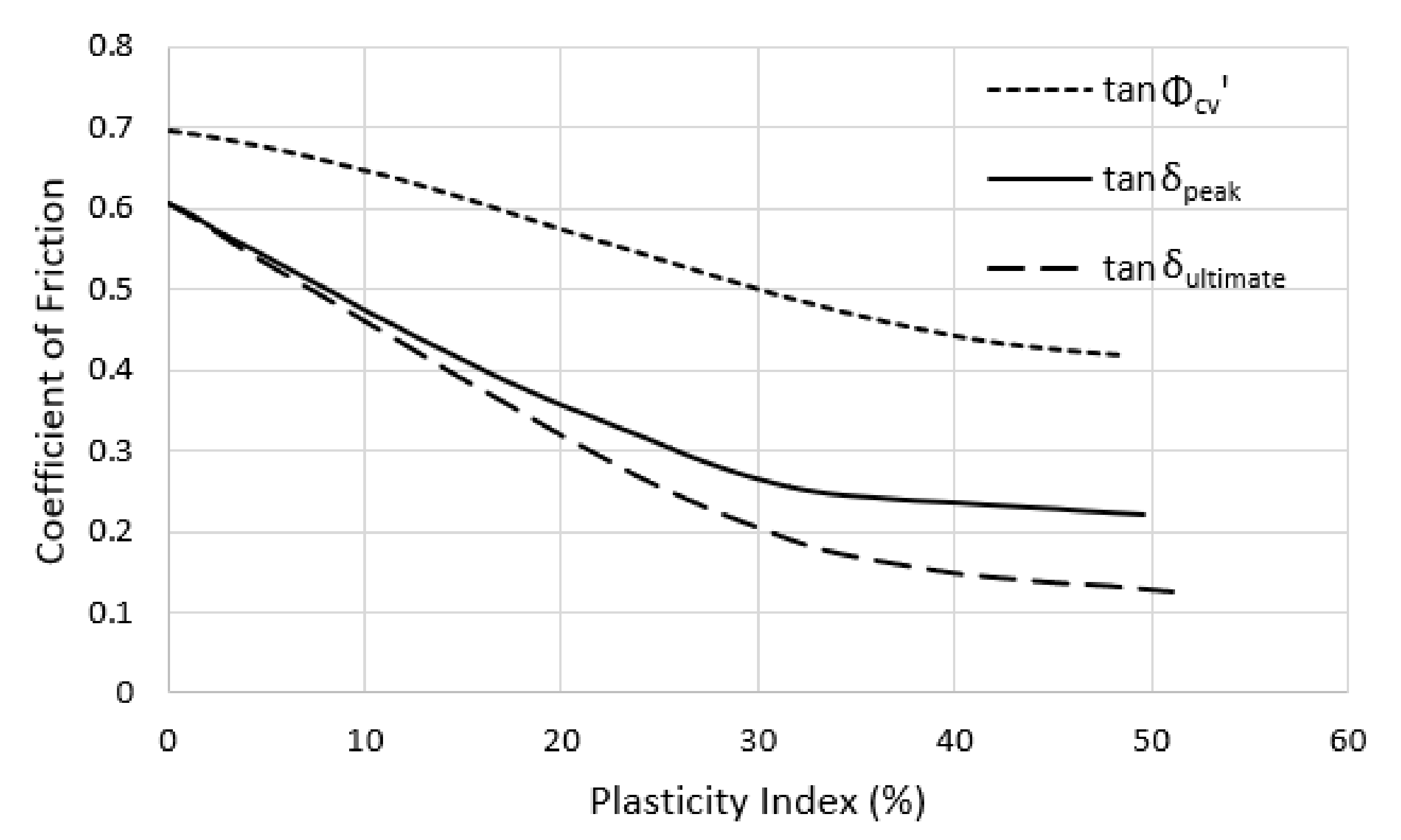
Figure 6.
The loading diagram of the first 10 cycles for the 8 MN one-way cyclic load.

Figure 7.
Mesh density, (a) 37,405 nodes model. (b) 56,932 nodes model.
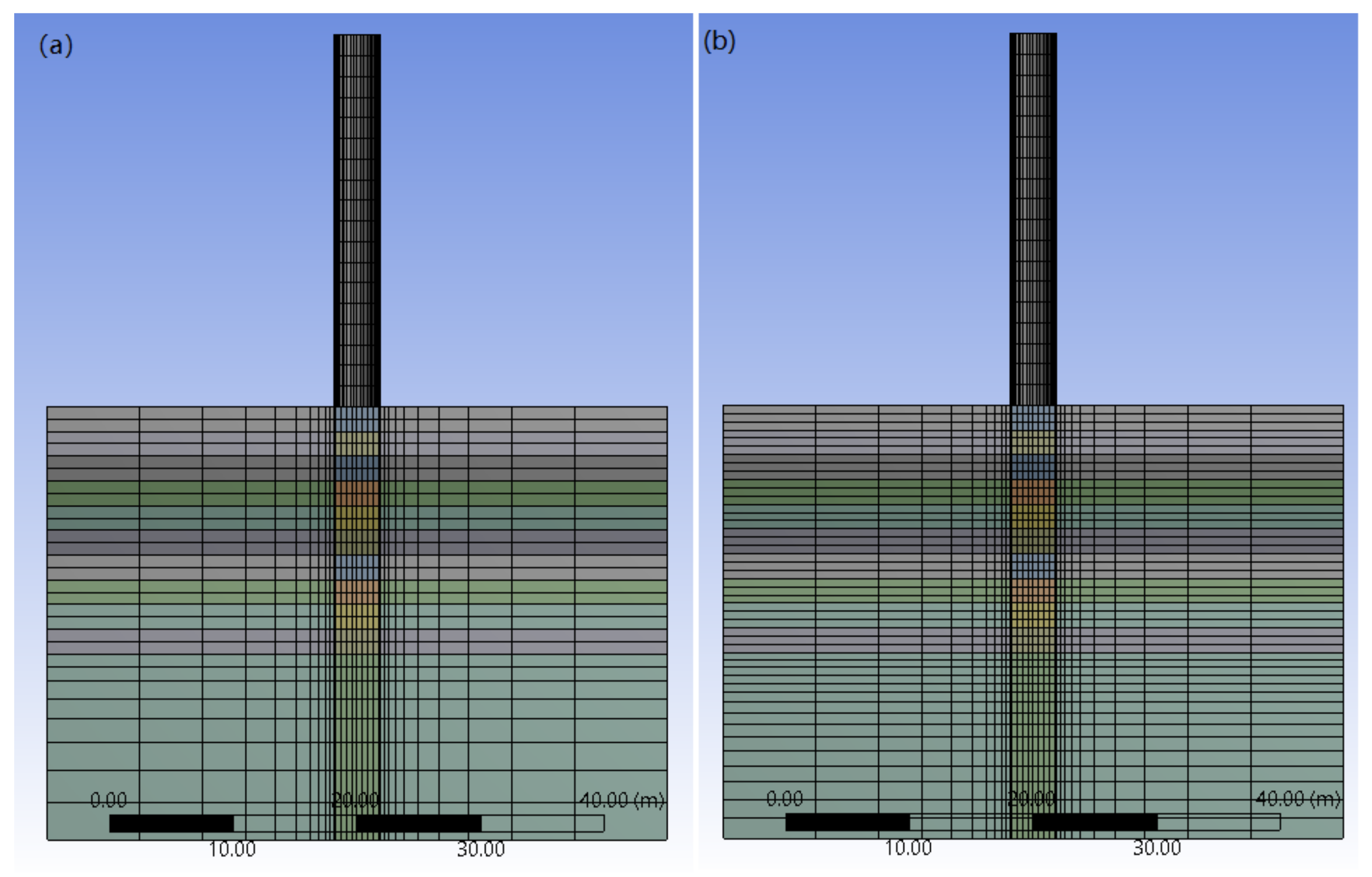
Figure 8.
Time history of the pile head displacement in the sensitivity analysis.

Figure 9.
Setup for the centrifuge test (after [16]).
Figure 9.
Setup for the centrifuge test (after [16]).

Figure 10.
Model with 11 layers of soil, used for validation with the centrifuge test.

Figure 11.
Validation of the monotonic model.
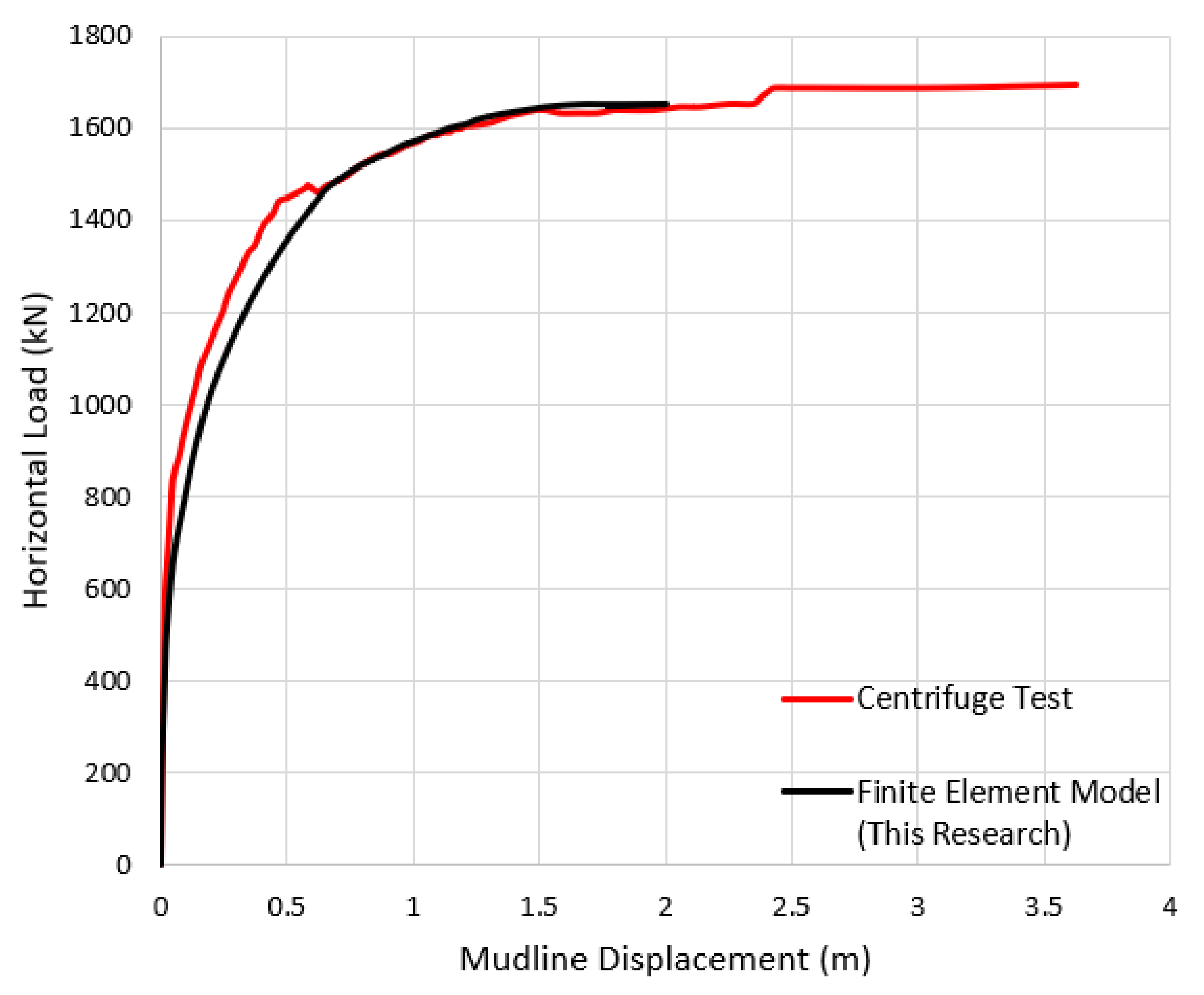
Figure 12.
Validation of the cyclic model.

Figure 13.
Time History of the rotation for the 17 simulations. (a) D = 5 m, L = 25 m. (b) D = 6.25 m, L = 25 m. (c) D = 7.5 m; L = 25 m. (c) D = 5 m, L = variable as shown.
Figure 13.
Time History of the rotation for the 17 simulations. (a) D = 5 m, L = 25 m. (b) D = 6.25 m, L = 25 m. (c) D = 7.5 m; L = 25 m. (c) D = 5 m, L = variable as shown.

Figure 14.
Relationship between D × L × ln(Cu) and the corresponding pile rotation in the first cycle (agreement from Equation (4)).
Figure 14.
Relationship between D × L × ln(Cu) and the corresponding pile rotation in the first cycle (agreement from Equation (4)).
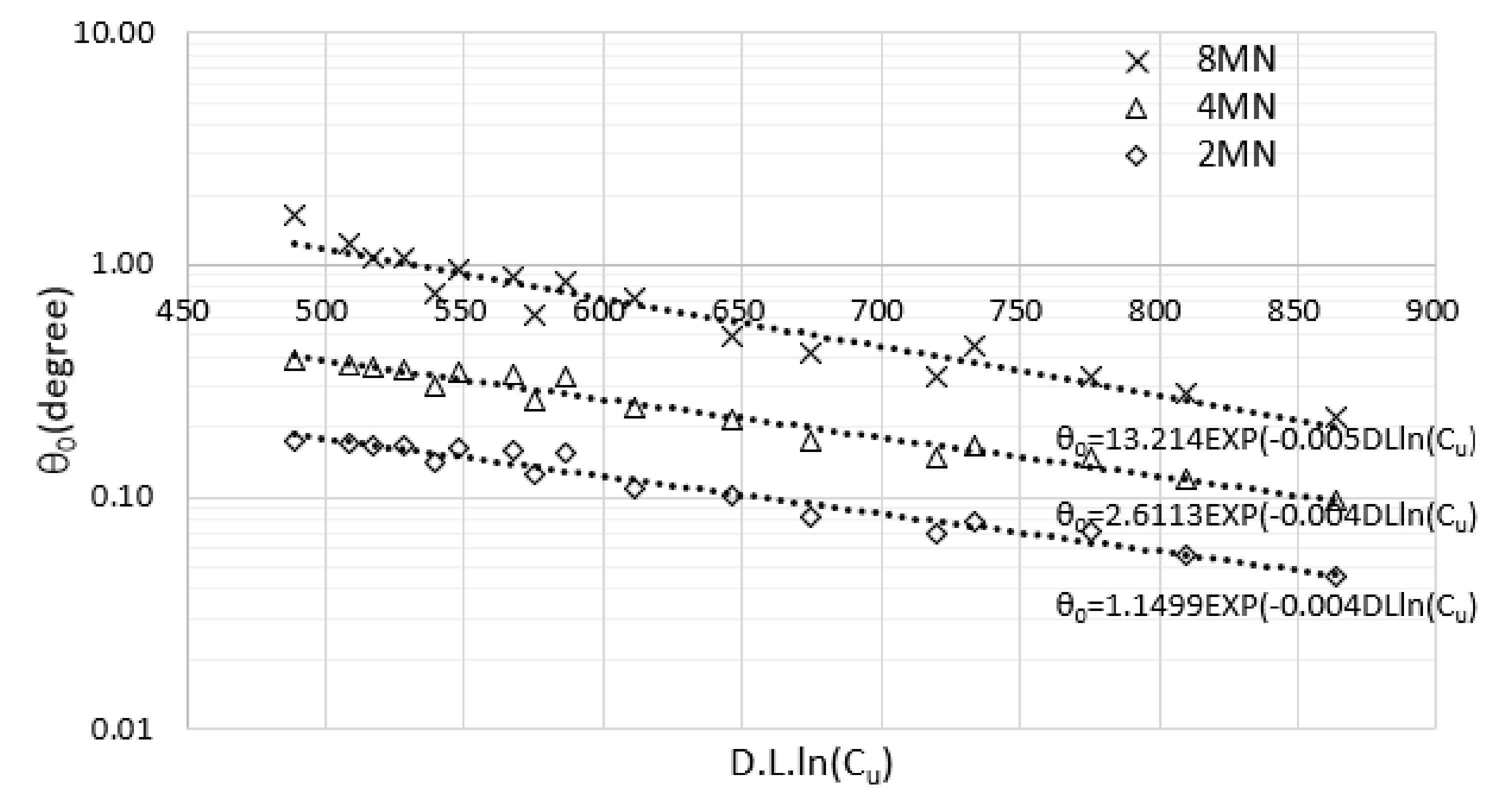
Figure 15.
Cumulative rate of rotation for different values of D × L × ln(Cu).

Figure 16.
The cumulative rate of rotation for the single amplitude and multi-amplitude models.

Table 1.
Pile geometrical properties.
| D—Pile Diameter (m) | tp—Pile Thickness (mm) | H—Total Pile-Structure Length (m) | L—Embedded Length (m) |
|---|---|---|---|
| 5.00 | 57 | 55 | 25–30 |
| 6.25 | 69 | 55 | 25 |
| 7.50 | 82 | 55 | 25 |
Table 2.
Pile material properties.
| Material | Density (kg/m3) | Young’s Modulus (kPa) | Poisson’s Ratio |
|---|---|---|---|
| Steel | 7850 | 200,000 | 0.3 |
Table 3.
Soil properties for the cyclic behaviour models (after [20]).
Table 3.
Soil properties for the cyclic behaviour models (after [20]).
| Clay Type | Unit Weight (kN/m3) | Plasticity Index (%) | Undrained Shear Strength (kPa) | Correction Factor, Kc | Young’s Modulus (kPa) |
|---|---|---|---|---|---|
| 1 | 44 | 50 | 383 | 19,150 | |
| 2 | 40 | 75 | 447 | 33,525 | |
| 3 | 18 | 38 | 100 | 479 | 47,900 |
| 4 (0–10 m depth) | 44 | 50 | 383 | 19,150 | |
| 4 (10–20 m depth) | 40 | 75 | 447 | 33,525 |
Table 4.
Coefficient of friction for each type of clay.
| Clay Type | Plasticity Index (%) | Coefficient of Friction |
|---|---|---|
| 1 | 44 | 0.240 |
| 2 | 40 | 0.247 |
| 3 | 38 | 0.250 |
| 4 (0–10 m depth) | 44 | 0.240 |
| 4 (⩾10 m depth) | 40 | 0.250 |
Table 5.
Five site conditions used in the test (after [16]).
Table 5.
Five site conditions used in the test (after [16]).
| Site | Layer 1 | Layer 2 | ||
|---|---|---|---|---|
| Depth a (m) | Consolidation Pressure (kPa) | Depth b (m) | Consolidation Pressure (kPa) | |
| A | 13.5 | 500 | 13.5 | 500 |
| B | 13.5 | 300 | 13.5 | 300 |
| C | 13.5 | 180 | 13.5 | 180 |
| D | 5.0 | 180 | 22.0 | 500 |
| E | 10.0 | 180 | 17.0 | 500 |
Table 6.
Experimental programme on the prototype scale (after [16]).
Table 6.
Experimental programme on the prototype scale (after [16]).
| Phase | Test Number | Test Nature | Pile Diameter (m) | Vertical Load (MN) | Site Specification |
|---|---|---|---|---|---|
| OWF-01 | 6.5 | B | |||
| I | OWF-02 | Monotonic | 3.83 | 6.5 | A |
| OWF-03 | 4.0 | C | |||
| OWF-04 | 4.0 | C | |||
| OWF-05 | 6.5 | B | |||
| II | OWF-06 | Cyclic | 7.62 | 6.1 | A |
| OWF-07 | 6.0 | D | |||
| OWF-08 | 6.1 | E | |||
| III | OWF-09 | Cyclic | 7.62 | 12.0 | A |
Table 7.
Stages and loading profiles for OWF-06 to OWF-09 (after [16]).
Table 7.
Stages and loading profiles for OWF-06 to OWF-09 (after [16]).
| Stage | OWF-06 | OWF-07 | OWF-08 | OWF-09 | ||||
|---|---|---|---|---|---|---|---|---|
| Min, Max Load (N) | No. of Cycles | Min, Max Load (N) | No. of Cycles | Min, Max Load (N) | No. of Cycles | Min, Max Load (N) | No. of Cycles | |
| 1 | 0, 3 | 1000 | 0, 3 | 1000 | 0, 3 | 1000 | 0, 6 | 1000 |
| 2 | −3.2, 36 | 1000 | 2, 32.5 | 1000 | 0.2, 31.2 | 1000 | −1, 60 | 1000 |
| 3 | −2.5, 79 | 1000 | −19.5, 56.5 | 500 | 3.6, 79 | 1000 | 5, 150 | 1000 |
| 4 | 0, 100 | 100 | −0.6, 100 | 500 | 10.6, 111 | 500 | 17.3, 223 | 1000 |
| 5 | NA | NA | −30, 123 | 479 | −30.6, 121 | 500 | −65, 238 | 500 |
| 6 | NA | NA | 14, 167.5 | 500 | −12.5, 140 | 500 | −86, 217 | 500 |
| 7 | Monotonic Push | |||||||
Table 8.
Input soil properties for validating the monotonic and cyclic behaviour (after [16]).
Table 8.
Input soil properties for validating the monotonic and cyclic behaviour (after [16]).
| Layer | Monotonic Behaviour Validation | Cyclic Behaviour Validation | |||||||
|---|---|---|---|---|---|---|---|---|---|
| Depth (m) | OCR | Kc | Cu (kPa) | E (kPa) | OCR | Kc | Cu (kPa) | E (kPa) | |
| 1 | 1 | 14.7 | 147.0 | 7.7 | 1126.4 | 14.7 | 147.0 | 24.0 | 3520.8 |
| 2 | 3 | 9.8 | 152.6 | 12.3 | 1879.2 | 9.8 | 152.6 | 27.1 | 4137.3 |
| 3 | 5 | 5.8 | 278.3 | 14.4 | 3998.4 | 5.8 | 278.3 | 35.9 | 9999.7 |
| 4 | 7 | 4.0 | 397.0 | 15.9 | 6301.1 | 10.4 | 147.0 | 44.6 | 6547.5 |
| 5 | 9 | 3.1 | 483.0 | 17.2 | 8326.7 | 8.0 | 197.7 | 46.9 | 9264.0 |
| 6 | 11 | 2.5 | 527.7 | 18.1 | 9530.9 | 6.5 | 251.0 | 50.2 | 12,607.2 |
| 7 | 13 | 2.1 | 561.7 | 18.6 | 10,453.4 | 5.5 | 293.0 | 54.4 | 15,948.2 |
| 8 | 15 | 1.8 | 579.6 | 19.2 | 11,103.3 | 4.7 | 341.0 | 56.3 | 19,205.9 |
| 9 | 17 | 1.6 | 589.2 | 19.7 | 11,608.8 | 4.0 | 394.0 | 60.9 | 24,012.6 |
| 10 | 19 | 1.3 | 597.3 | 21.2 | 12,668.1 | 3.5 | 441.0 | 65.4 | 28,823.3 |
| 11 | 20 | 1.3 | 599.5 | 22.0 | 13,206.5 | 3.3 | 454.0 | 67.9 | 30,817.9 |
Table 9.
Information on the dynamic models conducted study cyclic behaviour.
| Model No. | Pile Diameter, D (m) | Embedded Pile Length, L (m) | Undrained Shear Strength, Cu (kPa) | Number of Cycles, N |
|---|---|---|---|---|
| 1 | 5.00 | |||
| 2 | 6.25 | 25 | 50 | 100 |
| 3 | 7.50 | |||
| 4 | 5.00 | |||
| 5 | 6.25 | 25 | 75 | 100 |
| 6 | 7.50 | |||
| 7 | 5.00 | |||
| 8 | 6.25 | 25 | 100 | 100 |
| 9 | 7.50 | |||
| 10 | 5.00 | |||
| 11 | 6.25 | 25 | 50 & 75 | 100 |
| 12 | 7.50 | |||
| 13 | 26 | |||
| 14 | 27 | |||
| 15 | 5.00 | 28 | 50 | 100 |
| 16 | 29 | |||
| 17 | 30 |
Table 10.
Pile rotations in the first cycle for the 17 simulations.
| Model No. | Pile Diameter, D (m) | Embedded Pile Length, L (m) | Undrained Shear Strength, Cu (kPa) | D × L × ln(Cu) (m2 ln(kPa)) | Rotation 0 (Degree) |
|---|---|---|---|---|---|
| 1 | 5.00 | 489 | 1.65 | ||
| 2 | 6.25 | 25 | 50 | 611 | 0.72 |
| 3 | 7.50 | 734 | 0.45 | ||
| 4 | 5.00 | 540 | 0.76 | ||
| 5 | 6.25 | 25 | 75 | 675 | 0.42 |
| 6 | 7.50 | 810 | 0.28 | ||
| 7 | 5.00 | 576 | 0.61 | ||
| 8 | 6.25 | 25 | 100 | 720 | 0.33 |
| 9 | 7.50 | 863 | 0.22 | ||
| 10 | 5.00 | 517 | 1.07 | ||
| 11 | 6.25 | 25 | 62.5 | 646 | 0.49 |
| 12 | 7.50 | 775 | 0.33 | ||
| 13 | 26 | 509 | 1.24 | ||
| 14 | 27 | 528 | 1.08 | ||
| 15 | 5.00 | 28 | 50 | 548 | 0.96 |
| 16 | 29 | 567 | 0.89 | ||
| 17 | 30 | 587 | 0.85 |
Publisher’s Note: MDPI stays neutral with regard to jurisdictional claims in published maps and institutional affiliations. |
© 2021 by the authors. Licensee MDPI, Basel, Switzerland. This article is an open access article distributed under the terms and conditions of the Creative Commons Attribution (CC BY) license (https://creativecommons.org/licenses/by/4.0/).
Share and Cite
MDPI and ACS Style
Xie, M.; Lopez-Querol, S. Numerical Simulations of the Monotonic and Cyclic Behaviour of Offshore Wind Turbine Monopile Foundations in Clayey Soils. J. Mar. Sci. Eng. 2021, 9, 1036. https://doi.org/10.3390/jmse9091036
AMA Style
Xie M, Lopez-Querol S. Numerical Simulations of the Monotonic and Cyclic Behaviour of Offshore Wind Turbine Monopile Foundations in Clayey Soils. Journal of Marine Science and Engineering. 2021; 9(9):1036. https://doi.org/10.3390/jmse9091036
Chicago/Turabian StyleXie, Mian, and Susana Lopez-Querol. 2021. "Numerical Simulations of the Monotonic and Cyclic Behaviour of Offshore Wind Turbine Monopile Foundations in Clayey Soils" Journal of Marine Science and Engineering 9, no. 9: 1036. https://doi.org/10.3390/jmse9091036
Note that from the first issue of 2016, this journal uses article numbers instead of page numbers. See further details here.