An Integrated Strategy toward the Extraction of Contour and Region of Sonar Images


College of Marine Electrical Engineering, Dalian Maritime University, Dalian 116026, China
*
Authors to whom correspondence should be addressed.
J. Mar. Sci. Eng. 2020, 8(8), 595; https://doi.org/10.3390/jmse8080595
Submission received: 6 July 2020
/
Revised: 2 August 2020
/
Accepted: 6 August 2020
/
Published: 10 August 2020
(This article belongs to the Section Ocean Engineering)
Abstract
:In this paper, an integrated underwater sonar image extraction strategy, which combines two improved methods, namely the level set method (LSM) and the Lattice Boltzmann Method (LBM), is proposed. First, sonar images are processed by a clustering method and a connected domain analysis to generate the target minimum rectangle frame. Next, the segmentation task is decomposed into two subtasks, namely a coarse segmentation task to obtain the initial contour and a fine segmentation task after embedding the initial contour. Finally, the improved LSM is used to obtain the target contour, and the coarse contour of the segment is embedded into the LBM to obtain the region segmentation of the target in the sonar images. The main contributions of the paper are as follows: (1) The contours and regions of the sonar images are extracted simultaneously. (2) The original LBM method is enhanced to solve the level set iteration problem. (3) The region segmentation with the original image background is extracted, and a more intuitive region segmentation result than that of directly extracting the contour of the level set is achieved. Experimental results based on four evaluation indices of image segmentation show that our method is effective, accurate, and superior to other existing methods.
1. Introduction
Image segmentation is the key step from image processing to image analysis. In general, image segmentation methods can be summarized as threshold-based, region-based, edge-based, and some specific theory-based segmentation methods. These methods have their own characteristics. Image segmentation based on a threshold is simple and widely used, but it is difficult to obtain good segmentation when the image is complex. Most edge-based segmentation methods are applicable to the image with obvious edges. The edge segmentation results may have discontinuous edges, and it is highly desirable to obtain a continuous edge so as to obtain the overall contour of the target. In addition, there is a segmentation method based on neural networks, which requires a lot of image annotations and offline training. Unfortunately, there is no general sonar image data set that can support the training model.
Most of these image segmentation research object categories are optical or remote sensing images, and the research for underwater sonar image segmentation has always been a challenging problem. The correct segmentation of underwater sonar images is an important prerequisite for the development of seabed resources, underwater search and rescue, and the classification and recognition of seabed geology and other activities. Hence, it is highly important to study the segmentation of sonar images. At the same time, we notice that the contour information of a target is the most concise way to describe the target, among which the level set method (LSM) is used widely and has a great prospect.
The LSM in [1] is a kind of numerical technology for interface tracking and shape modeling. It is also robust to deal with noise images and has been applied in the field of image processing. By using this method, we can obtain the shape feature and contour of the target in a sonar image, which is the most clear and simple way to represent the image. We can use the contour to carry out image feature training. At the same time, through the segmentation of the level set, we can also obtain the area part of the target and measure the size of the target in proportion.
Compared with the previous active contour model [2,3,4], the LSM has been changed into an implicit representation, raising the calculation of low dimension to higher dimension. Although the amount of calculation has increased relatively, there are many advantages about this method, and it is used widely. For example, first, the problem will be simplified when topology changes in the low dimension are applied to a high dimension. Second, the steps of reinitialization are omitted in the high dimension space relative to the low dimension space. Third, when this implicit representation is used to solve PDEs, there are mature operation tools in a high-dimensional space.
Compared with the geodesic active contour model, the LSM shows good performance, and some images that are not suitable for classical snake method (based on gradient) segmentation are successfully segmented [5,6,7]. This method is also extended to the segmentation of texture images [8]. With the application of the LSM in image fields widely studied by scientists, a large number of classical theories have emerged [9,10,11,12,13]. A comparative study of eight deformable contour methods in medical image segmentation is summarized in [2], showing the versatility, advantages, and disadvantages of various deformable contour methods comprehensively, such as gradient vector flow snake, original level set, and so on. The experience and lessons from the comparison of these methods about medical segmentation can also be applied to other fields of image segmentation.
Recently, some new methods have also been used to replace the LSM [14,15,16,17,18,19]. In order to enhance the noise robustness of the standard method, the authors in [20,21] embedded the Markov random field (MRF) energy function into the conventional energy function of the level set. This proposed model has parallel processing ability.
All of the aforementioned methods have achieved satisfactory results in image segmentation. Although the LSM has been actively studied in the field of image segmentation, there is an unsolved issue in sonar image segmentation. Because of the characteristics of sonar images, such as noise, uneven gray distribution, and unclear edges, we believe that the LSM can segment a sonar image target more quickly and clearly than other segmentation methods. Of course, neural networks methods are also very popular in recent years, but the huge and tedious offline labelling and training work makes this method not suitable for practical applications, especially when there is no general sonar image data set. Hence, our research focuses on the improvement of the LSM and how to better improve the segmented visual experience. To our knowledge, the latest research literature of the LSM for sonar image segmentation are [22,23,24], and an expectation–maximization (EM) approach assisted by Dempster–Shafer evidence theory (DST) for image segmentation is presented in [25]. All these methods deal with the noise reduction of sonar images and segmentation. The purpose of segmentation is to divide a sonar image into three parts, including the target, background, and shadow. Different from these existing methods, in this paper, we use the LSM to segment the target so as to remove the background and shadow. We want to use the LSM to obtain the continuous target contour, which is conducive to our subsequent underwater target feature training. We notice that there is still relatively early sonar image segmentation work [26], but the segmentation result is a single area form, which is not conducive to the comprehensive observation of sonar images.
Even though the LSM has a great advantage over other methods in dealing with noise, it is still not applicable to all sonar images. Although the evolution speed of the Distance Regularized Level Set Evolution (DRLSE) model in [11] has been greatly improved, we find that a direct application of this model to noisy images still has drawbacks, and most of the level set initialization of the manual or random mode will lead to inaccurate segmentation results.
In this context, a novel method to segment real-world sonar images is proposed. The proposed method integrates two existing technologies, namely the LSM and the Lattice Boltzmann method (LBM).
Because the numerical scheme (such as the finite difference method) used in the LSM will limit the time step, the number of iterations in the LSM is large, and the calculation is complex. We notice that the LBM is a common method in physical hydrodynamics, which is rarely used in image segmentation. Furthermore, compared with other region segmentation methods, such as texture segmentation, it can be used for large-area classification problem like seabed topography. Threshold segmentation [27] can only present several gray-level block regions according to the selection of the threshold. There are also some examples of using filters [27] to segment images. These common classical region segmentation methods are more suitable for optical images [28]. In view of the uneven distribution and high noise of sonar images, we introduce the LBM to segment the region. It turns out that the LBM is suitable for the problem at hand as evidenced by the experimental results. Hence, we employed it in sonar image segmentation to observe the region segmentation of sonar images, embedded it in our level set initialization improvement algorithm, and obtained good results with a few iterations. Finally, the method shows the segmentation effect, including the original image background and the target, and it solves the problem that the segmentation effect is only the contour or the pure area extracted directly from the contour, which is conducive to a comprehensive observation of the target.
Since the pixels far away from the object contour are meaningless for obtaining the object boundary and will increase the computational load, the sonar image is coarsely segmented by removing the unnecessary background and shadow first. In this way, the number of evolution iterations and time can be saved. The minimum rectangular contour of the target in the sonar image, which can be embedded as the initial evolution curve of the level set, is accordingly obtained.
The main ideas of the proposed strategy are as follows: First, sonar images are processed by the clustering method and connected domain analysis [28] to generate the target minimum rectangle frame. The minimum bounding rectangle is embedded into the initialization process of the LSM (we termed the uniform operation as the cluster connected analysis), which is the precondition to generate a minimum bounding rectangle of the target in sonar images. The energy equation of the LSM is subsequently redesigned so as to eliminate the deviation caused by setting the initial contour randomly or manually. Next, the region segmentation of the sonar images can be combined with the LBM, which can be used to segment the target with an original background. This is beneficial to our overall observation. Finally, the information of the contour and the region of underwater sonar images is presented, and the objective of obtaining the region and contour information of the target in sonar images is achieved. Experimental studies show that the accuracy of segmentation is improved, and the number of iterations is reduced significantly by using the proposed method. The main contributions of this paper are as follows: (1) To overcome the shortcomings of traditional LSM, which needs a random setting or manual definition of an initial contour, the minimum bounding rectangle of the target domain can be embedded automatically as the initial contour of the level set. (2) The evolution accuracy is improved by dividing the sonar image segmentation into two subtasks, namely a coarse segmentation of the cluster connected analysis and a fine segmentation of the curve evolution. (3) The LSM and LBM are improved respectively and integrated; the former is applied to fine segmentation to obtain the target contour, while the latter is used to obtain the region segmentation of the target in sonar images.
The paper is organized as follows. Section 2 gives an overview of our framework, including the traditional level set model, the DRLSE model, and LBM. Section 3 introduces the proposed integration method and its theoretical knowledge in detail. In Section 4, experimental studies demonstrate that the performance of our method on synthetic, natural, and sonar images is superior. Concluding remarks are drawn in Section 5.
2. Preliminaries
As foreshadowed, the proposed strategy combines two classical methods, namely the LSM and LBM. To facilitate the understanding of the proposed strategy, the preliminaries pertaining to the LSM and LBM are reviewed here.
2.1. Traditional Level Set Model
This traditional level set model was proposed in [1]. Specifically, the singularity problem in the general equation of curve evolution, which is as follows,
was solved in [1], where represents a two-dimensional curve, is the time, denotes the normal component of the velocity of motion, is the speed of motion, and is the unit normal vector of a two-dimensional curve. The implicit expression of a planar closed curve C is used to extend it from the level set of a two-dimensional Cartesian coordinate function :
where the extension is made to the zero-level set of a three-dimensional continuous function surface, defined on the image as follows:
where denotes the image pixel.
For any given contour curve, the level set function begins to evolve under the influence of the velocity field. The specific level set evolution function can be expressed as follows:
The above equation is the basic equation of the LSM for curve evolution, which depends on the image data and the level set function.
2.2. DRLSE Model
The DRLSE model in [11] was proposed by Li C. et al. Given that Ω is set as the image area and as the level set function defined on I, the energy function of the DRLSE model is expressed as
where the first item is the penalty item, and it guarantees the smoothness of the level set curve in the evolution process. The second item is the length item, and the third item is the area item. These items guide the evolution of the level set to the target boundary. The constants μ, λ, and v are the weighting coefficients for each energy term, while (∙) is the energy density function, is the gradient operator, (∙) denotes the Dirac functions, and (∙) denotes the Heaviside functions. The edge stop
function is defined as
where is the Gaussian kernel of the parameter σ, and is the image function.
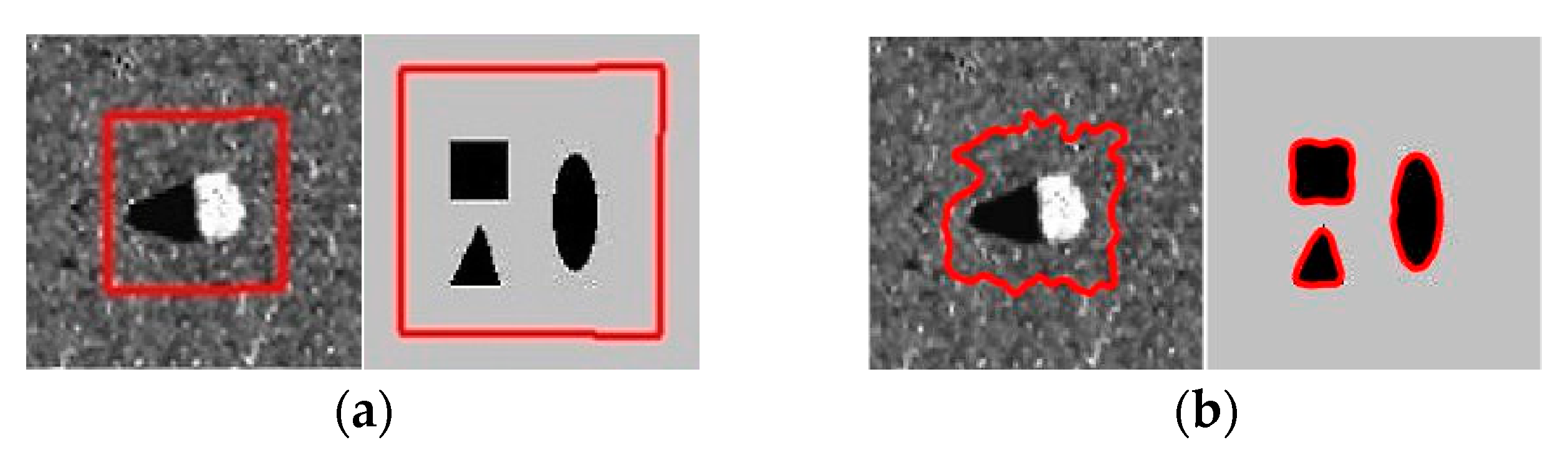
This DRLSE model sometimes fails to segment images in cases when either there is noise, the edge is not obvious, or the background is complex. As shown in Figure 1, the experiment on a simple image shows that the method segments the target successfully, but the target is not segmented effectively when replaced with a noisy image or an uneven gray-scale image. In addition, it should be highlighted that the sonar images in this paper are all public from the website.
We set different initial modes by using traditional methods and may obtain different segmentation results, which makes the work of image segmentation difficult.
When we increase the number of iterations from 300 to 500, this also fails to segment the contour of the target correctly, implying that the DRLSE model is seriously affected by noise in an image.
2.3. Lattice Boltzmann Model
The Lattice Boltzmann method (LBM) has been used as an alternative to solve level set equations (LSE) recently [29]. Because of the simplicity of the algorithm and the implicit calculation of curvature, the height can be parallelized, which can handle time-consuming problems better.
The equation of the LBM evolution in [30] can be written as follows using Bhatnagar, Gross, and Krook collision models:
Each link has its velocity vector and a particle distribution that moves along this link where is the position of the cell, is the time, and represents the relaxation time of a fluid that determines the kinetic viscosity ϑ,
and is a balanced particle distribution, which is defined as
where to are constants, depending on the geometry of the lattice chain, denotes the macroscopic fluid density, and denotes velocities calculated from the particle distribution:
where is the discrete velocity distribution function, which represents the particle density when the velocity is .
In a typical diffusion calculation model case, the balanced function can be simplified as follows:
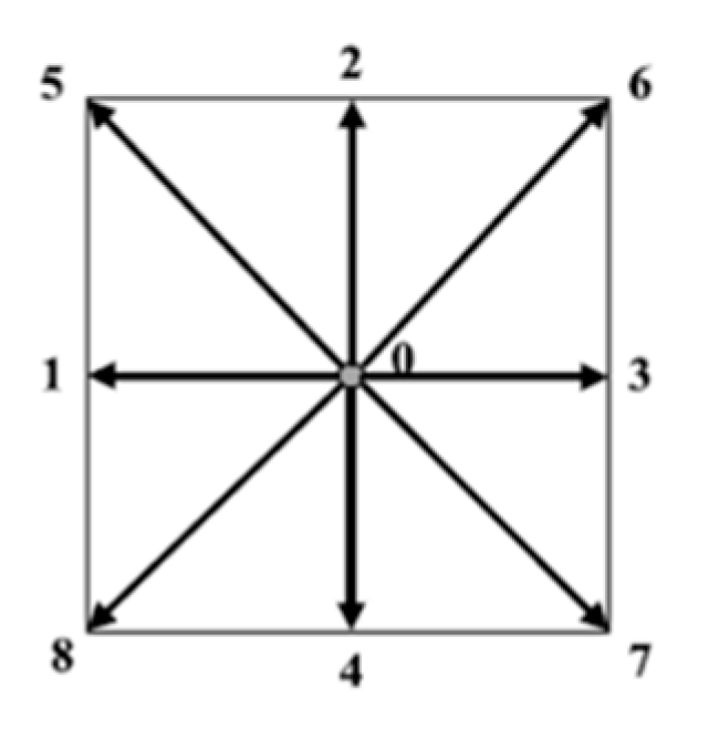
Our strategy uses (2D with eight links in its neighbors and one link in its cell) cell structure of LBM. Figure 2 shows a typical model [30].
The model has zero links , axial connections , and diagonal links . The relaxation time τ is determined by the diffusion coefficient γ, which is defined as
The LBM can be used to solve a parabolic diffusion equation, which can be recovered by the following Chapman–Enskog expansion:
In this case, external forces can be included in the LBM after the collision computation as
where is the body force. Thus, Equaction (13) becomes
and the LSE can be restored by replacing ρ with the sign distance function Φ.
3. The Proposed Strategy
3.1. An Overview
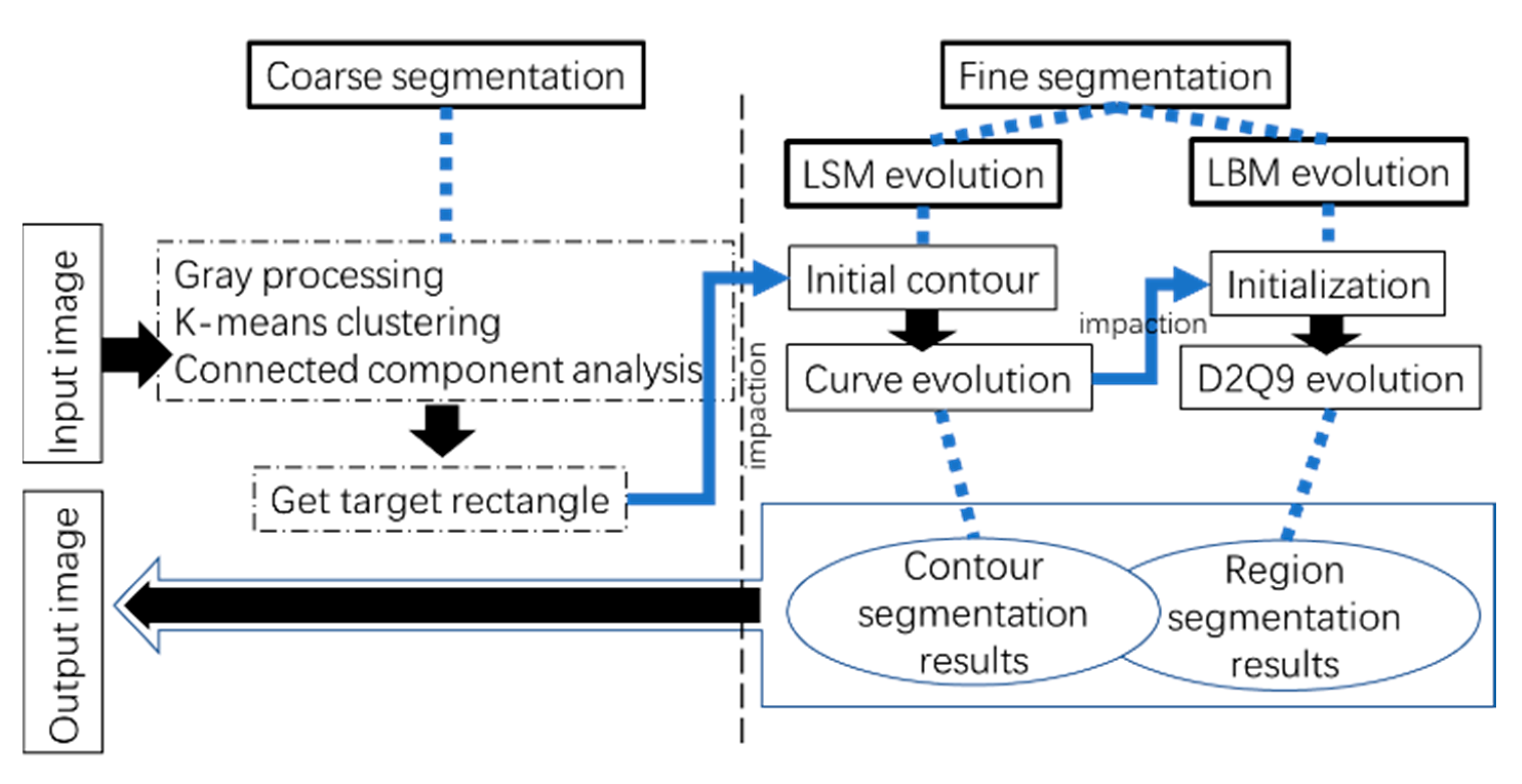
To solve the aforementioned problems, we fix the initialization term and embed it in the initial energy function of the level set, which is represented in the image as the minimum bounding rectangle. We first apply the method of rectangle generation, which is a combination of cluster analysis and connected region analysis. Next, we start the evolutionary process. This strategy can overcome the randomness of manual initialization. At the same time, we import the coarse contour of the target into the LBM and apply it to the segmentation of sonar images. Finally, this integration method not only obtains the contour information of the underwater target, but it also obtains the region segmentation with an image background. Finally, the accuracy and speed of target segmentation can be improved greatly by our strategy.
The flow diagram of this framework is shown in Figure 3.
By using the proposed strategy, the complexity and the computational load can be reduced significantly, and the segmentation accuracy of sonar images is improved greatly by combining the improved level set and LBM.
3.2. Coarse Segmentation
3.2.1. K-Means
Assuming that the input samples are where represent the number of objects in the sample, the algorithm steps are as follows: Given that the centers of K clusters are , and the number of samples in each cluster is , the square error function is regarded as the following objective function [31]:
For of each sample, we mark it as the category closest to the category center, and we have the following:
We update the center of each category to the mean of all samples belonging to that category as follows:
This function is a convex function about , and its stagnation point is calculated as follows:
Repeat the next two steps until the category center changes less than a certain threshold. When the objective function reaches the minimum value, the iteration is stopped.
In our research, the clustering method is only a part of the simple application of coarse segmentation of sonar images. Hence, we chose the classical K-means clustering method, which can achieve fast coarse segmentation of images.
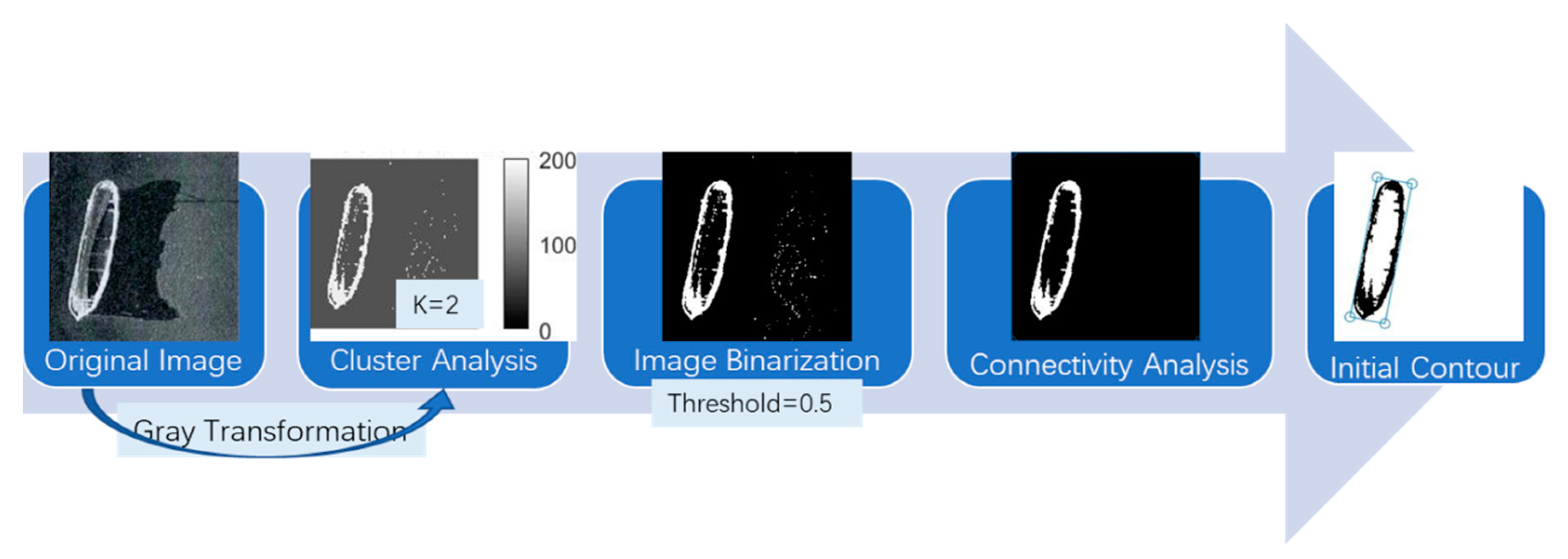
Since the K-means clustering only needs to play a role in the coarse segmentation of sonar images, our framework needs the number of clusters (K = 2) in K-means clustering. Figure 4 shows the core process of initial contour acquisition. The test image is transformed into its gray level, and the gray histogram of the image is presented. Through a large number of experiments in the early stage, aiming at the characteristics of sonar images in this paper, the binarization threshold is between 0.45 and 0.5. Using this threshold, we can automatically extract a large connected area through the code to obtain the main body of the target.
3.2.2. Acquisition of Initialization Curve
In order to obtain an appropriate initial evolution curve, the minimum bounding rectangle is constructed. By using a cluster connected analysis of the sonar images, their coordinates are obtained and embedded. Because the target boundary is almost covered by the initial contour, the level set is defined as an inward evolution, which can be regarded as an appropriate initial evolution curve. The number of iterations is reduced using the initial evolution curve based on shape knowledge. Our sonar images can be represented by
where is a normal number, is the image region, represents the area enclosed by the minimum initial rectangle contour at this moment (it should be noted that once the evolution begins, will continue to change until it reaches the desired edge), and is the minimum bounding rectangle after applying a
cluster connected analysis of the sonar images. Table 1 shows the initial coordinate points generated after clustering connection.
3.3. Fine Segmentation
3.3.1. Improved Energy Equation
In the fine segmentation, we embed the initial contour, which is obtained by our strategy in Figure 4, and the evolution equation is redesigned as follows:
where is the rate of evolution. Once the evolution begins, will be refreshed as the evolution contour continuously.
The basic equation of curve evolution can be changed to
where is the unit normal vector of the two-dimensional curve, and the function is the normal component of the velocity, which depends on the image data and the level set function.
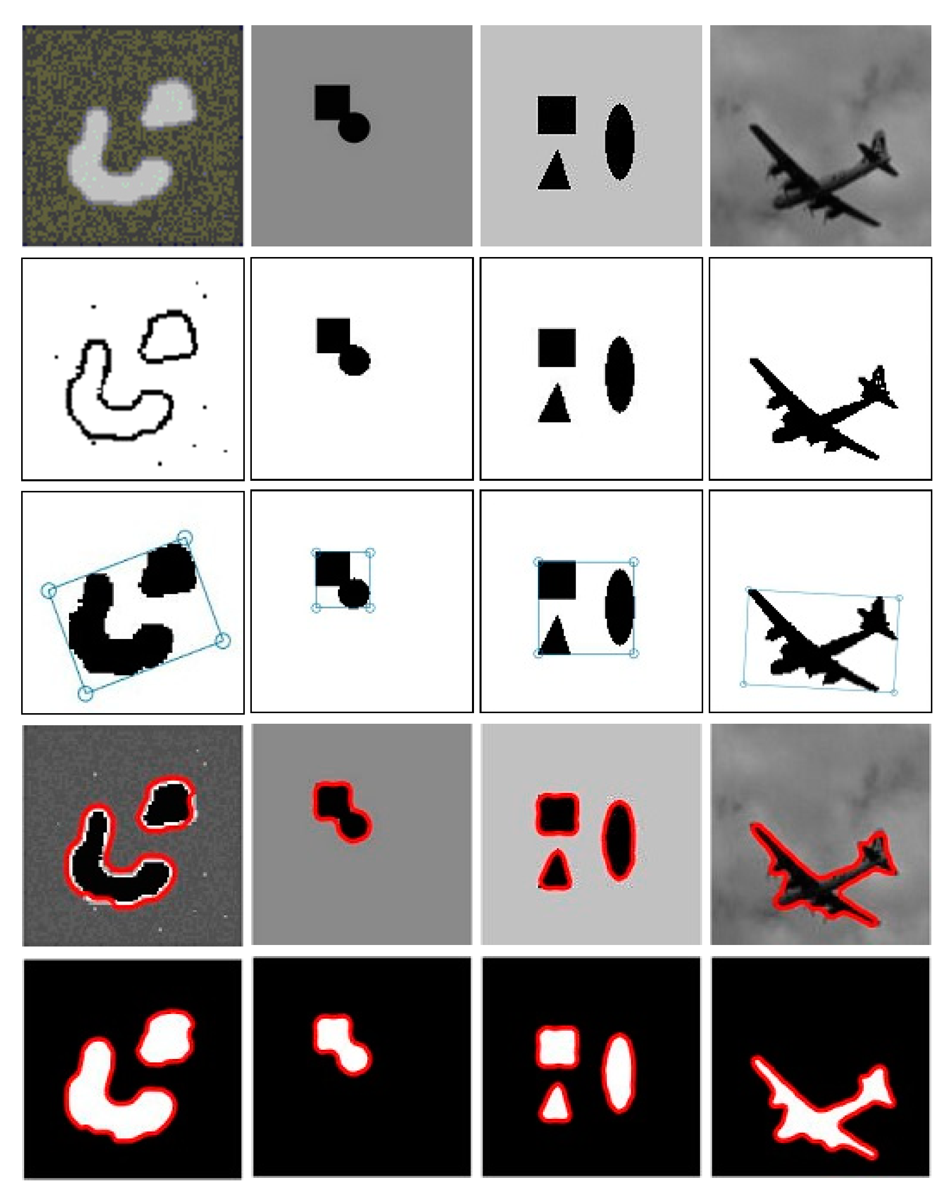
We verify the availability of our method on some the simple images and optical images given in Figure 5. It can be seen from Figure 5 that our improved LSM has been verified in both the simple and optical images successfully. In the next step, this method will be applied to some challenging sonar image segmentation and compared with some existing methods.
3.3.2. Importing LBM
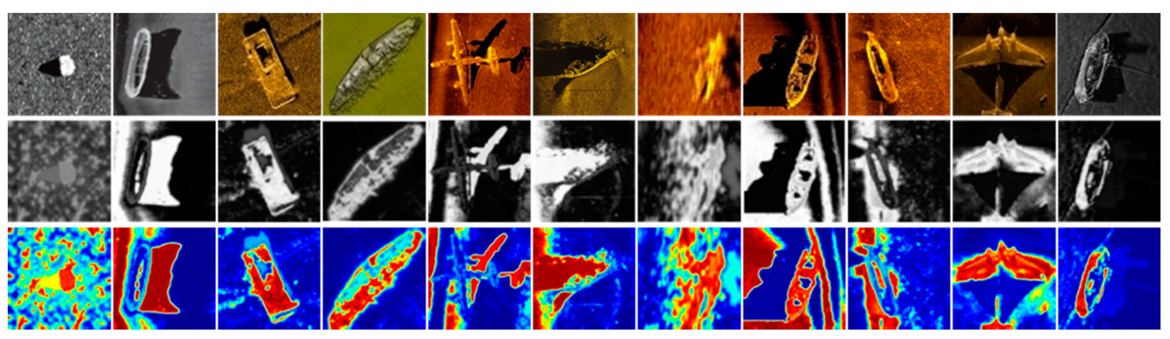
Region segmentation of the sonar images can be obtained by the LBM. Combined with our improved LSM, we can observe image contour and region segmentation with a background simultaneously so that we can analyze the segmentation results more comprehensively. There is a problem that needs attention when using the LBM. If the initial contour of the LBM is generated randomly, it can achieve good results in simple images, but it can hardly achieve correct segmentation in sonar images because the gray distribution of a general sonar image is uneven and contains much noise. Figure 6 shows a failed sonar image segmentation initialized in a random way by the LBM.
Based on the problems in the above experiments, we propose a strategy that embeds the coarse contour of the improved level set evolution into the LBM as the initial evolution contour. Only a few iterations are needed to obtain the target region segmentation. In this paper, the rough contour of a sonar target is defined as . Next, the evolution energy function of LBM is written as
where represents the relaxation time of the fluid that determines the kinematic viscosity :
and is the equilibrium particle distribution, which is defined as
where to are constants that are dependent on the geometry of the lattice chain; and and are, respectively, the macroscopic fluid densities and velocities calculated from the particle distribution:
For a typical diffusion calculation model, the equilibrium function can be simplified as follows:
4. Experimental Results and Analysis
This section is divided into five parts. In the first part, we compare the region segmentation results of our LBM with that of the random initial contour LBM to show the effectiveness of our method intuitively. The second part shows the initial contour generated by the cluster connected analysis. In the third part, we compare the final evolution curve of the improved level set with five other LSMs. The fourth part lists the number of iterations in a table. In the fifth part, four evaluation indices are used to evaluate our method and other parallel methods, and we analyze the accuracy and advantages of our strategy used in real images objectively and quantitatively.
It should be emphasized that the LBM is introduced into the region segmentation of images. Compared with the contour segmentation of the level set, the LBM can obtain accurate region segmentation directly with a few iterations in the case of an image background. This kind of region segmentation is more suitable for subjective observation, while the contour result of the level set is conducive to data evaluation. Even a simple contour can be used to train the shape characteristics of specific underwater objects, which is conducive to underwater object recognition and classification. This is also the reason why the two methods are used together in this paper. The information in sonar images is analyzed comprehensively and objectively from human visual subjective data.
Due to the limitation of having few sonar image data sets, most of the research on sonar image target extraction is a single data set. There is a data set including 8 sonar images in [23], which contains noise and nonuniform intensity sonar images, and the size and variance of those are given. This is a relatively comprehensive data set with description that we found. We use 11 sonar images with noise and uneven intensity. If compared with images of the same size, our image variance is larger and more challenging than the eight images in [23].
To demonstrate the effectiveness and efficiency of our method, we provide the mean and standard deviation of the 11 sonar images in Table 2. Through the data of Table 2 and real sonar images, we can see that the segmentation work is indeed challenging.
4.1. Comparison of LBM Evolution
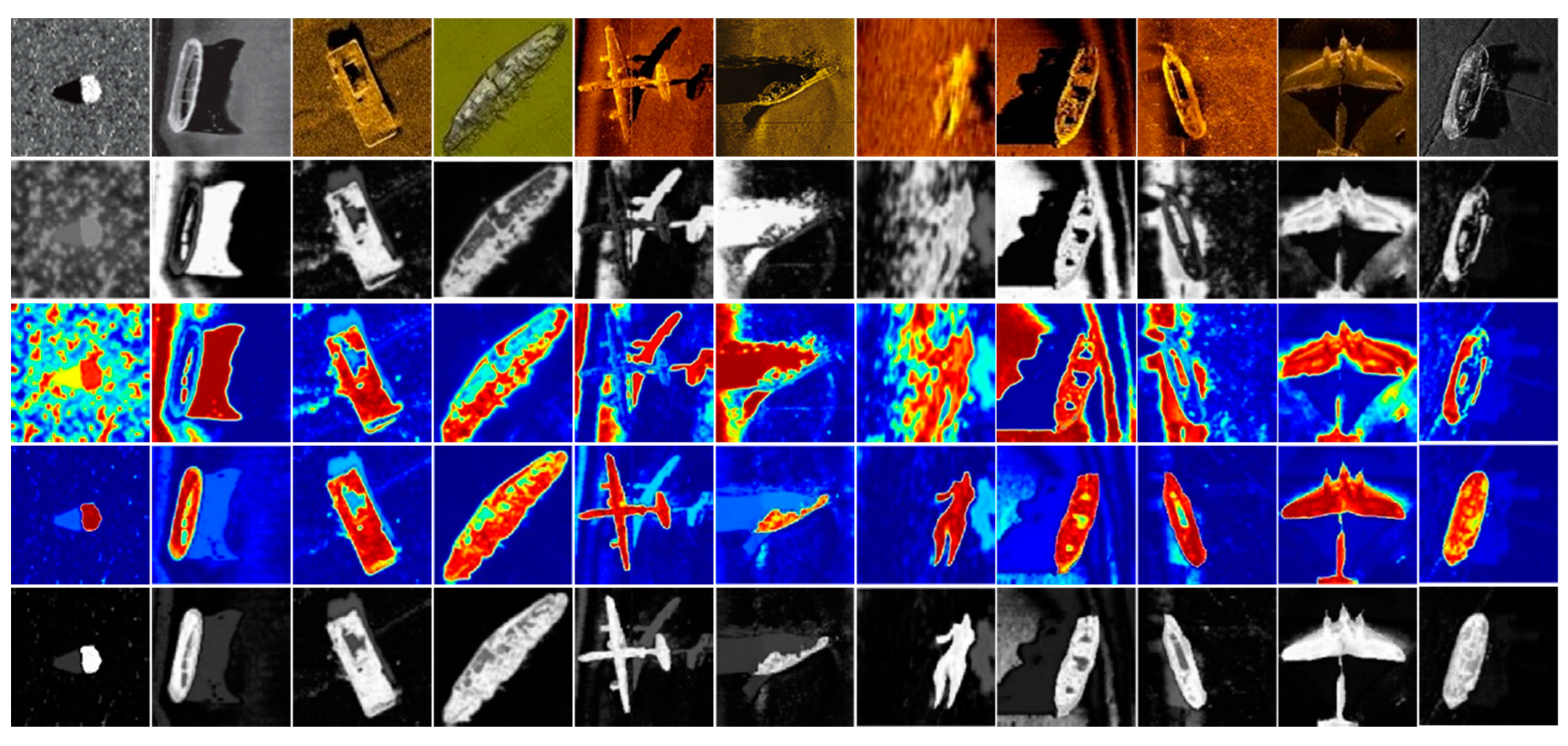
The original LBM uses an automatically generated circle as the initial contour. Our Lattice Boltzmann evolution uses our proposed initial contour, which is embedded in the level set. It can be seen from Figure 7 that the segmentation of the first, sixth, seventh, and eighth images in the second and third rows respectively are not successful, and other segmentation effects are not ideal. This is due to the limitations of traditional methods and the diversity of our data set. However, in the actual task for sonar image segmentation, it is impossible to have all simple images. Hence, our data set is reasonable, and it is necessary to expand the diversity of the data set. If the improved method can be used in complex image segmentation, the effectiveness of our improvement method will be further shown.
The fourth to the fifth rows show our improved LBM segmentation. It can be seen that the segmentation results of our improved LBM are significantly improved compared with the original segmentation of the second to the third rows.
4.2. Generation of Initial Contour of LSM
4.3. Comparison of Level Set Evolution
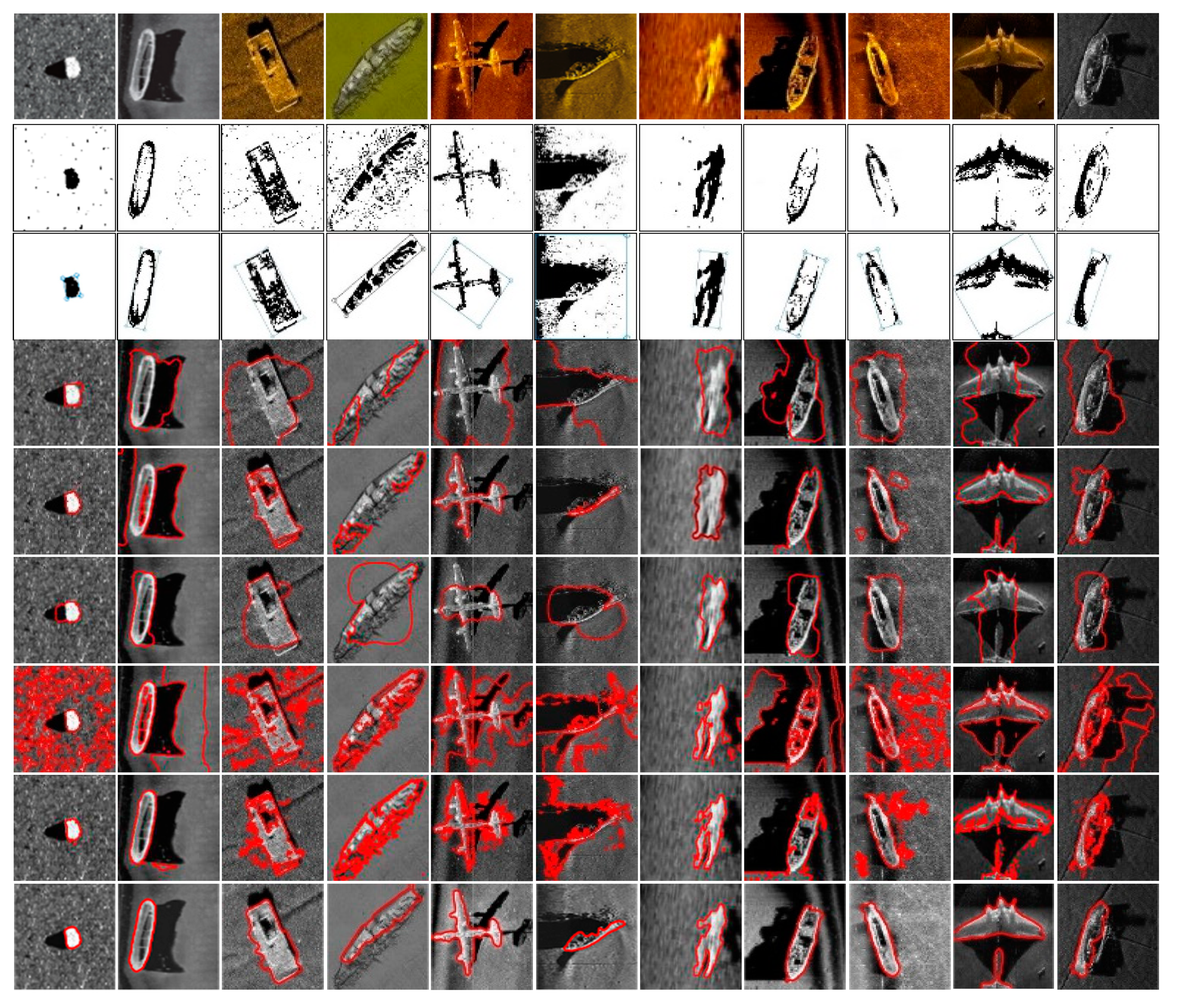
As shown in Figure 9, we compared our level set method with other classical level set methods. In order to obtain a better segmentation effect for other methods, we manually selected the initial contour closer to the target than that which we automatically generated. It should be emphasized that the research work on LSM for sonar image segmentation is very rare. The important literature we have found are [22,23,24,25], but their work is devoted to the segmentation of three parts instead of removing the background and shadow. This is very different from our research purpose. Therefore, our comparative test does not include these recent studies.
By comparing the segmentation results in the visual observation images, we can see that our method is concise and clear in segmenting the contour of the target generally. Other traditional methods have great limitations in sonar image segmentation.
4.4. Analysis of Number of Iterations
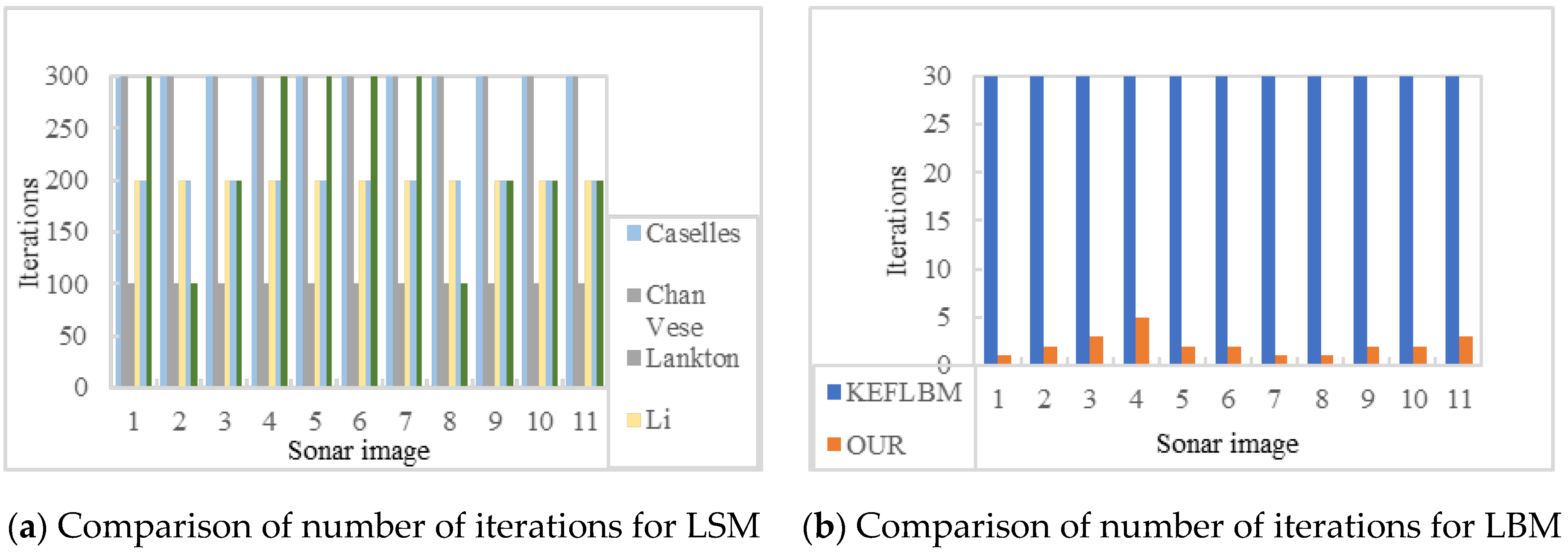
After intuitively analyzing the segmentation results, we compared and analyzed the number of iterations of the experiment here. Figure 10 lists the number of iterations of six LSMs and two LBMs respectively. The X-axis represents the test sonar image number for the experiment, and the Y-axis represents the number of iterations. The image sequence is the same as the first line in Figure 7. By analyzing the number of iterations for LSE, we can see that the average number of iterations set by our method are at the middle level, and the number of iterations of Lankton’s method is significantly lower because the method itself is an experiment based on the local energy of an active contour. According to the corresponding image results in Figure 9, we can see that Lankton’s method is not suitable for complex underwater sonar images because regardless of how many iterations we set, we will not get satisfactory results. Due to the fact that Shi’s method emphasizes the real-time computation of the algorithm, which is a great advantage, our method is committed to accurately segmenting the contour and area of the target in the sonar image, which lays a solid foundation for subsequent research works. Because the sonar images we have chosen are diverse, we can increase the number of iterations properly in more complex images to obtain better segmentation results. This can be seen in Figure 10b. When we use our LBM strategy to segment regions, the number of iterations is greatly reduced. At the same time, we can conclude that the comparative test in part B of this section, i.e., our LBM region segmentation strategy, shows good segmentation results.
4.5. Performance Evaluation
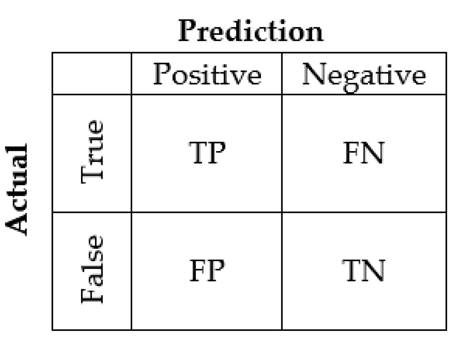
We select several common evaluation indices (Dice, Jaccard, precision, and recall) for image segmentation [33] to evaluate the segmentation results. The three evaluation indices of Dice, precision, and recall involve the principle of confusion matrix [34]. The formula and schematic diagram are described in Figure 11.
The significance of the four evaluation indices is as follows:
- 1.
- Dice coefficient: It is a set similarity measurement function, which is usually used to calculate the similarity of two samples (value range is [0, 1]). The larger the value is, the closer the results of the two samples are. It is given by the following:
- 2.
- Precision: Represents the accuracy of the forecast results, given by
- 3.
- Recall: Represents the comprehensiveness of the forecast results, and it is given by the following [35]:
- 4.
- Jaccard: It is used to compare the similarity and difference between finite sample sets. It is the ratio of the intersection and union of two given sets A and B. The larger the Jaccard value is, the higher the similarity is, as given by
The input images are SEG (which represents experimental segmentation results) and GT (ground truth). We need to take out the corresponding categories in SEG and GT from the segmented images and use the function to calculate the category separately.
We select the representative level set as the Chan-Vese (CV) method [7] and the Lankton method [12] from the image experiment shown in Figure 9 for quantitative comparison. The methods proposed in these two studies have been widely used in the past decade, and the number of citations has reached thousands. Up to now, they have been cited 107 times and 9 times respectively in 2020, which is enough to illustrate the practicability and durability of the two data comparison methods. The results are shown in Table 3. Recently, a novel method using a superellipse active contour has been proposed [36]. However, this paper mainly focuses on the recognition and classification of naval mines. It should be highlighted that a superellipse does not always perfectly track the shapes in very noisy input data. Hence, based on the high noise characteristics of our sonar images, we do not compare our work with this method. However, it should still be noted that the superellipse parameters are sufficiently described in the very noisy input data case so that a successful classification of naval mines can be achieved. In the future work of classification and recognition of sonar images, we will conduct an in-depth study on this.
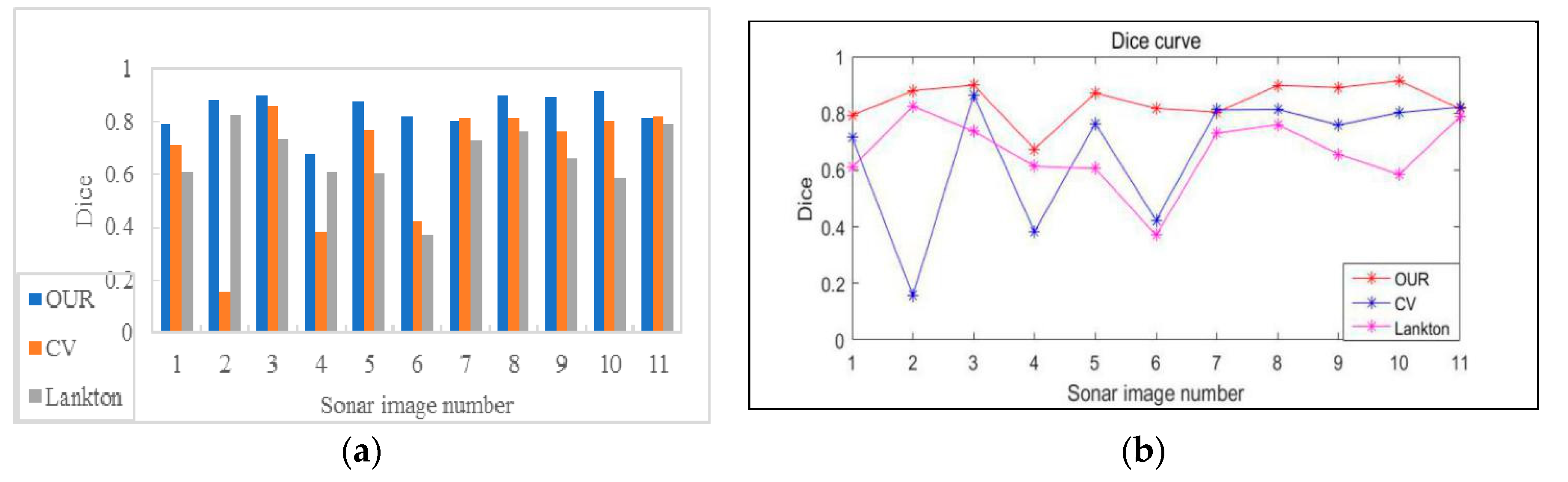
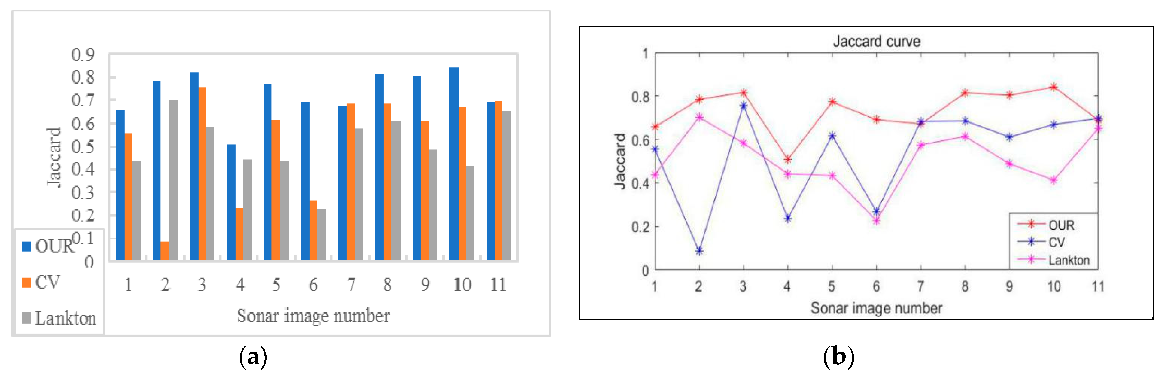
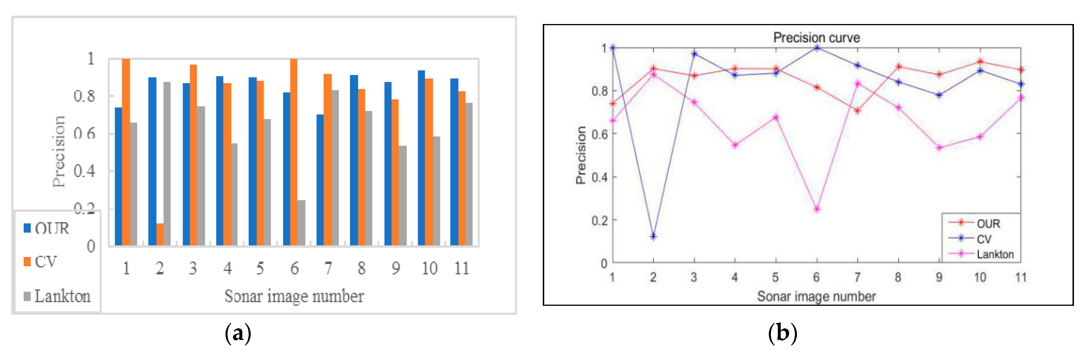
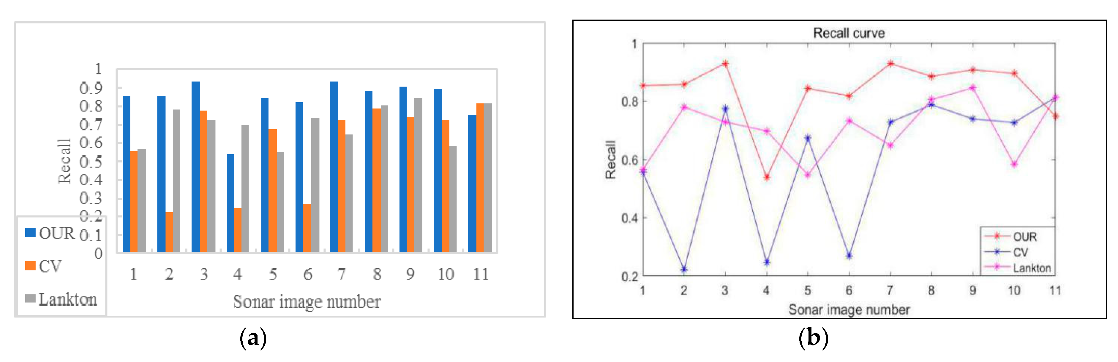
We transformed the data results into a histogram and line graph [37,38] in order to facilitate observation and comparison. As shown in Figure 12, Figure 13, Figure 14 and Figure 15, we can see that our method is accurate and effective in most cases by listing the evaluation results. Because precision and recall are two relative evaluation indices and are contradictory, we regard them as better segmentation, as their values are higher at the same time. We calculated the average value of four evaluation indices of the three methods respectively, and the results are shown in Table 4. We can see that the average value of our strategy is higher than other methods.
At the same time, by observing the evaluation results of the line chart, we can see that our strategy is more consistent than both CV and Lankton’s when the sonar images are segmented. There are great fluctuations in the recall value of CV. Generally speaking, our method has advantages in both visual image results and numerical evaluation results, which further proves the effectiveness of our strategy.
The above experiment is the best result we have obtained, although the problem also involves some algorithm parameters (smooth Gaussian kernel parameters, filter parameters, time step), and each parameter has substantive significance, which may affect the final result. However, what we want to emphasize here is that the new method proposed in this paper is effective and efficient to segment the contour and region information of sonar images simultaneously.
5. Conclusions
In this paper, a novel strategy for sonar image segmentation was devised. Not only was the typical LSM applied and improved by us, but also the improved LBM was extended to sonar image segmentation. To summarize, first, the sonar images were preprocessed based on the clustering method. After eliminating the discrete points, the connectivity domain of the target was analyzed to obtain the minimum bounding rectangle, which is different from the original contour randomly set or manually defined by the classical LSM. Next, we embedded the contour of the level set evolution and obtained a fine segmentation of the target in the sonar images by iterations. The segmentation task is divided into two subtasks, namely coarse segmentation using a cluster connected analysis and fine segmentation of curve evolution. During the fine segmentation process, we used the improved LSM to obtain the target contour, and then used the improved LBM to obtain the region segmentation of the target with the original image background. Finally, the integrated segmentation of the sonar images is achieved by extracting the continuous edge contour of the target and the shape features of the area. We tested the proposed strategy on simple composite images and sonar images, and four indices of image segmentation evaluation were used to evaluate the segmentation results. The results demonstrate that the proposed method not only provides abstract contour information and area shape features of the image, but it also accelerates the speed of curve evolution and improves the segmentation accuracy. Experimental results show that our strategy is accurate and effective for the challenging task of the segmentation of sonar images.
Author Contributions
Conceptualization, H.X. and W.L.; methodology, software, and investigation, W.L.; resources, H.X. and W.L.; writing—original draft preparation, W.L.; writing—review and editing, M.J.E., H.X. and W.L.; visualization, W.L.; supervision, H.X. and M.J.E.; project administration, M.J.E. and H.X. All authors have read and agreed to the published version of the manuscript.
Funding
This research received no external funding.
Conflicts of Interest
The authors declare no conflict of interest.
References
- Osher, S.; Sethian, J.A. Fronts propagating with curvature-dependent speed: Algorithms based on Hamilton-Jacobi formulations. J. Comput. Phys. 1988, 79, 12–49. [Google Scholar] [CrossRef] [Green Version]
- He, L.; Peng, Z.; Everding, B.; Wang, X.; Han, C.Y.; Kenneth, L.W.; William, G.W. A comparative study of deformable contour methods on medical image segmentation. Image Vis. Comput. 2008, 26, 141–163. [Google Scholar] [CrossRef]
- Kass, M.; Witkin, A.; Terzopoulos, D. Snakes: Active contour models. Comput. Vis. 1988, 1, 321–331. [Google Scholar] [CrossRef]
- Xu, C.; Prince, J.L. Snakes shapes and gradient vector flow. IEEE Trans. Image Process. 1988, 7, 359–369. [Google Scholar] [CrossRef] [Green Version]
- Wang, B.; Yuan, X.; Gao, X.; Li, X.; Tao, D. A Hybrid Level Set With Semantic Shape Constraint for Object Segmentation. IEEE Trans. Cyber. 2019, 49, 1558–1569. [Google Scholar] [CrossRef] [PubMed]
- Han, Y.; Zhang, S.; Geng, Z.; Wei, Q.; Ouyang, Z. Level set based shape prior and deep learning for image segmentation. IET Image Process. 2020, 14, 183–191. [Google Scholar] [CrossRef]
- Chan, T.F.; Vese, L.A. Active contours without edges. IEEE Trans. Image Process. 2001, 10, 266–277. [Google Scholar] [CrossRef] [Green Version]
- Sagiv, C.; Sochen, N.A.; Zeevi, Y.Y. Integrated active contours for texture segmentation. IEEE Trans. Image Process. 2006, 15, 1633–1646. [Google Scholar] [CrossRef]
- Li, C.; Kao, C.; Gore, J.C.; Ding, Z. Minimization of Region-Scalable Fitting Energy for Image Segmentation. IEEE Trans. Image Process. 2008, 17, 1940–1949. [Google Scholar] [CrossRef] [Green Version]
- Li, C.; Huang, R.; Ding, Z.; Gatenby, J.C.; Metaxas, D.N.; Gore, J.C. A level Set Method for Image Segmentation in the Presence of Intensity Inhomogeneities With Application to MRI. IEEE Trans. Image Process. 2011, 20, 2007–2016. [Google Scholar] [CrossRef]
- Li, C.; Xu, C.; Gui, C.; Fox, M.D. Distance Regularized Level Set Evolution and Its Application to Image Segmentation. IEEE Trans. Image Process. 2010, 19, 3243–3254. [Google Scholar] [CrossRef] [PubMed]
- Lankton, S.; Tannenbaum, A. Localizing Region-Based Active Contours. IEEE Trans. Image Process. 2008, 17, 2029–2039. [Google Scholar] [CrossRef] [PubMed] [Green Version]
- Shi, Y.; Karl, W.C. A Real-Time Algorithm for the Approximation of Level-Set-Based Curve Evolution. IEEE Trans. Image Process. 2008, 17, 645–656. [Google Scholar] [CrossRef] [PubMed]
- Luo, S.; Tong, L.; Chen, Y. A Multi-Region Segmentation Method for SAR Images Based on the Multi-Texture Model With Level Sets. IEEE Trans. Image Process. 2018, 27, 2560–2574. [Google Scholar] [CrossRef] [PubMed]
- Yang, X.; Gao, X.; Tao, D.; Li, X. Improving Level Set Method for Fast Auroral Oval Segmentation. IEEE Trans. Image Process. 2014, 23, 2854–2865. [Google Scholar] [CrossRef]
- Khadidos, A.; Sanchez, V.; Li, C. Weighted Level Set Evolution Based on Local Edge Features for Medical Image Segmentation. IEEE Trans. Image Process. 2017, 26, 1979–1991. [Google Scholar] [CrossRef]
- Yang, X.; Gao, X.; Tao, D.; Li, X.; Li, J. An Efficient MRF Embedded Level Set Method for Image Segmentation. IEEE Trans. Image Process. 2015, 24, 9–21. [Google Scholar] [CrossRef]
- Chen, Y.; Chen, G.; Wang, Y.; Dey, N.; Sherratt, R.S.; Shi, F. A Distance Regularized Level-Set Evolution Model Based MRI Dataset Segmentation of Brain’s Caudate Nucleus. IEEE Access 2019, 7, 124128–124140. [Google Scholar] [CrossRef]
- Wang, D. Efficient level-set segmentation model driven by the local GMM and split Bregman method. IET Image Process. 2019, 13, 761–770. [Google Scholar] [CrossRef]
- Lianantonakis, M.; Petillot, Y.R. Sidescan sonar segmentation using active contours and level set methods. Eur. Oceans 2005 2005, 719–724. [Google Scholar] [CrossRef]
- Gao, M.; Chen, H.; Zheng, S.; Fang, B. Feature fusion and non-negative matrix factorization based active contours for texture segmentation. Signal Process. 2019, 159, 104–118. [Google Scholar] [CrossRef]
- Liu, Y.; Li, Q.; Huo, G. Robust and fast-converging level set method for side-scan sonar image segmentation. J. Electron. Imaging 2017, 26, 063021.1–063021.11. [Google Scholar] [CrossRef]
- Huo, G.; Yang, S.X.; Li, Q.; Zhou, Y. A Robust and Fast Method for Sidescan Sonar Image Segmentation Using Nonlocal Despeckling and Active Contour Model. IEEE Trans. Cybern. 2017, 47, 855–872. [Google Scholar] [CrossRef] [PubMed]
- Wang, X.; Guo, L.; Yin, J.; Liu, Z.; Han, X. Narrowband Chan-Vese model of sonar image segmentation: A adaptive ladder initialization approach. Appl. Acoust. 2016, 113, 238–254. [Google Scholar] [CrossRef]
- Fei, T.; Kraus, D. An evidence theory supported expectation-maximization approach for sonar image segmentation. In Proceedings of the International Multi-Conference on Systems, Signals & Devices, Chemnitz, Germany, 20–23 March 2012; pp. 1–6. [Google Scholar] [CrossRef]
- Yue, X.; Zhang, Z.; Liu, P.X.; Guan, H. Sonar image segmentation based on GMRF and level-set models. Ocean Eng. 2010, 37, 891–901. [Google Scholar] [CrossRef]
- Wawrzyniak, N.; Wlodarczyk-Sielicka, M.; Stateczny, A. MSIS sonar image segmentation method based on underwater viewshed analysis and high-density seabed model. In Proceedings of the 18th International Radar Symposium (IRS), International Radar Symposium, Prague, Czech Republic, 28–30 June 2017. [Google Scholar]
- Tomislav, M.; Ivan, A.; Željko, H.; Dieter, K. Real-time biscuit tile image segmentation method based on edge detection. ISA Trans. 2018, 76, 246–254. [Google Scholar] [CrossRef]
- Yan, Z.; Sun, Y.; Jiang, J.; Wen, J.; Lin, X. Novel explanation, modeling and realization of Lattice Boltzmann methods for image processing. Multidim. Syst. Sign. Process. 2015, 26, 645–663. [Google Scholar] [CrossRef]
- Chen, J.; Chai, Z.; Shi, B.; Zhang, W. Lattice Boltzmann method for filtering and contour detection of the natural images. Comput. Math. Appl. 2014, 68, 257–268. [Google Scholar] [CrossRef]
- Anitha, U.; Malarkkan, S. Sonar image segmentation and quality assessment using prominent image processing techniques. Appl. Acoust. 2019, 148, 300–307. [Google Scholar] [CrossRef]
- Abu, A.; Diamant, R. Unsupervised Local Spatial Mixture Segmentation of Underwater Objects in Sonar Images. IEEE J. Ocean. Eng. 2019, 44, 1179–1197. [Google Scholar] [CrossRef]
- Chen, L.; Bentley, P.; Mori, K.; Misawa, K.; Fujiwara, M.; Rueckert, D. DRINet for Medical Image Segmentation. IEEE Trans. Med. Imaging 2018, 37, 2453–2462. [Google Scholar] [CrossRef] [PubMed]
- Wang, D. Extremely Optimized DRLSE Method and Its Application to Image Segmentation. IEEE Access 2019, 7, 119603–119619. [Google Scholar] [CrossRef]
- Kuijf, H.J.; Biesbroek, J.M.; De Bresser, J.; Heinen, R.; Andermatt, S.; Bento, M.; Berseth, M.; Belyaev, M.; Cardoso, M.J.; Casamitjana, A.; et al. Standardized Assessment of Automatic Segmentation of White Matter Hyperintensities and Results of the WMH Segmentation Challenge. IEEE Trans. Med. Imaging 2019, 38, 2556–2568. [Google Scholar] [CrossRef] [PubMed] [Green Version]
- Köhntopp, D.; Lehmann, B.; Kraus, D.; Birk, A. Classification and Localization of Naval Mines With Superellipse Active Contours. IEEE J. Ocean. Eng. 2019, 44, 767–782. [Google Scholar] [CrossRef]
- Abu, A.; Diamant, R. Enhanced Fuzzy-Based Local Information Algorithm for Sonar Image Segmentation. IEEE Trans. Image Process. 2020, 29, 445–460. [Google Scholar] [CrossRef] [PubMed]
- Song, Y.; He, B.; Zhao, Y.; Li, G.; Sha, Q.; Shen, Y.; Yan, T.; Nian, R.; Lendasse, A. Segmentation of Sidescan Sonar Imagery Using Markov Random Fields and Extreme Learning Machine. IEEE J. Ocean. Eng. 2019, 44, 502–513. [Google Scholar] [CrossRef]
Figure 1.
Results in random initialization mode using the DRLSE method. (a) Random initial contours; (b) segmentation results of DRLSE.
Figure 1.
Results in random initialization mode using the DRLSE method. (a) Random initial contours; (b) segmentation results of DRLSE.

Figure 2.
Typical model. Here, is the dimension and is the number of speed components.

Figure 3.
Flow diagram of framework.

Figure 4.
Core process of initial contour generation.

Figure 5.
Improved method validation experiment. The first row: Original sonar images. The second row: Clustering analysis of images. The third row: Initial evolution contours after removing the discrete points. The fourth row: Our improved level set method. The fifth row: Extraction of target contour.

Figure 6.
Failure segmentation of the original Lattice Boltzmann method (LBM). The first row: Original sonar images. The second row: Segmentation results of the random initial LBM. The third row: Color images of the second row. It can be seen that using the LBM to segment sonar images directly will lead to wrong segmentation.

Figure 7.
Comparison of LBM evolution tests. The first row: Original sonar images. The second to the third rows: Random initial LBM segmentation results (line 3 shows the same result color map as line 2). The fourth to the fifth rows: Segmentation with our LBM strategy.
Figure 7.
Comparison of LBM evolution tests. The first row: Original sonar images. The second to the third rows: Random initial LBM segmentation results (line 3 shows the same result color map as line 2). The fourth to the fifth rows: Segmentation with our LBM strategy.

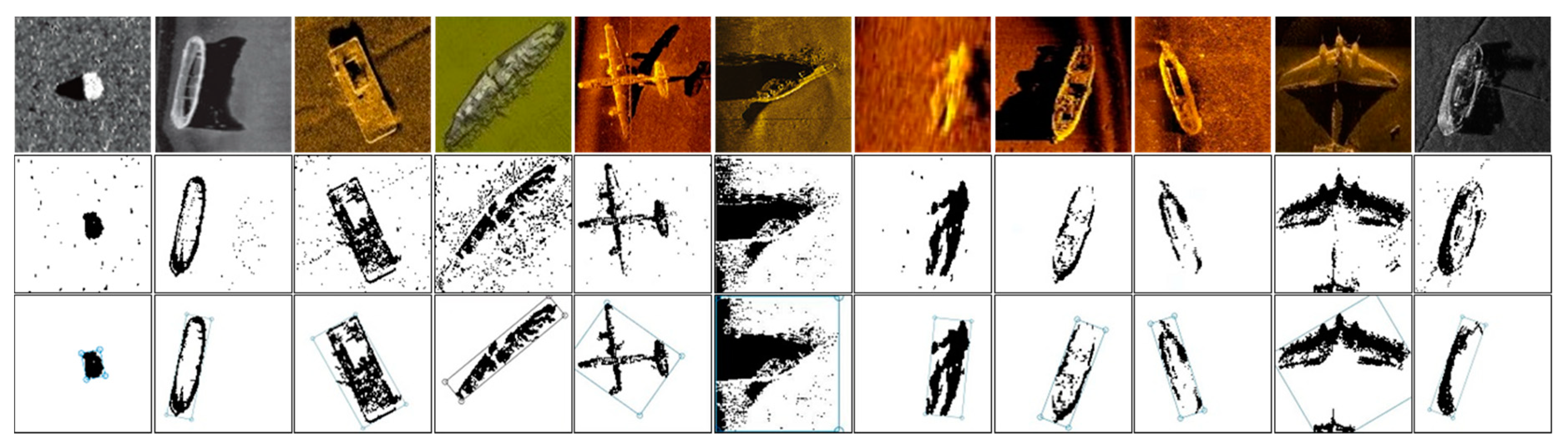
Figure 8.
Initial evolution contour generation experiment. The first row: Original sonar images. The second row: Image clustering analysis. The third row: The initial evolution contours obtained after removing the spurious points.
Figure 8.
Initial evolution contour generation experiment. The first row: Original sonar images. The second row: Image clustering analysis. The third row: The initial evolution contours obtained after removing the spurious points.

Figure 9.
Segmentation of sonar images by the level set method. The first row: Original sonar images (1–11). The second row: Images generated after clustering analysis. The third row: Minimum initial contours generated by the connected domain analysis after removing the straggling points [32]. The fourth to the eighth rows: Comparative tests by using five traditional level set methods (Casells method, Chan Vese method, Lankton method, Li method, and Shi method.) The ninth row: Results of our improved level set method on sonar image segmentation.

Figure 10.
Comparison of number of iterations for the level set equation (LSE) and LBM. Data set is the same as the eleven sonar images listed in Figure 7.
Figure 10.
Comparison of number of iterations for the level set equation (LSE) and LBM. Data set is the same as the eleven sonar images listed in Figure 7.

Figure 11.
In the confusion matrix, T/F indicates the right or wrong prediction, and P/N indicates the result of prediction. Prediction represents the predicted value, which is equivalent to the result of the test set (with possibly wrong results), and actual represents the real label (equivalent to the ground truth).

Figure 12.
Dice curve. (a) Histogram of Dice. (b) Line chart of Dice.

Figure 13.
Jaccard curve. (a) Histogram of Jaccard. (b) Line chart of Jaccard.

Figure 14.
Precision curve. (a) Histogram of precision. (b) Line chart of precision.

Figure 15.
Recall curve. (a) Histogram of recall. (b) Line chart of recall.


Table 1.
Initial contour coordinate point of level set evolution.
| Image Number | Coordinate Position | |||
|---|---|---|---|---|
| 1 | (81,52) | (86,76) | (68,80) | (63,55) |
| 2 | (30,18) | (53,22) | (34,117) | (11,112) |
| 3 | (58,19) | (105,103) | (65,125) | (18,41) |
| 4 | (107,1) | (122,19) | (25,99) | (10,81) |
The pixels of the images we used have been normalized to 128 × 128.
Table 2.
Mean and standard deviation of test images.
| Image Number | Mean | Standard Deviation |
|---|---|---|
| 1 | 96.8832 | 32.5612 |
| 2 | 89.3967 | 37.9007 |
| 3 | 77.1312 | 31.549 |
| 4 | 101.5292 | 19.2469 |
| 5 | 63.8182 | 35.5697 |
| 6 | 68.1406 | 30.9686 |
| 7 | 83.4479 | 34.9014 |
| 8 | 39.4496 | 41.2706 |
| 9 | 79.4364 | 31.4706 |
| 10 | 40.183 | 30.5781 |
| 11 | 49.8593 | 31.1562 |
Table 3.
Evaluation results (with the pixels test image that was used normalized to 128 × 128).
| Evaluation Indices | Dice | Jaccard | Precision | Recall | ||||||||
|---|---|---|---|---|---|---|---|---|---|---|---|---|
| Test image | OUR | CV | Lankton | OUR | CV | Lankton | OUR | CV | Lankton | OUR | CV | Lankton |
| Sonar1 | 0.7927 | 0.7146 | 0.609 | 0.6566 | 0.556 | 0.4378 | 0.7399 | 1 | 0.6597 | 0.8536 | 0.556 | 0.5655 |
| Sonar2 | 0.8794 | 0.1573 | 0.8248 | 0.7847 | 0.0854 | 0.7018 | 0.9018 | 0.1221 | 0.8751 | 0.858 | 0.2212 | 0.7799 |
| Sonar3 | 0.8988 | 0.8627 | 0.7365 | 0.8163 | 0.7585 | 0.583 | 0.8692 | 0.9715 | 0.7446 | 0.9306 | 0.7758 | 0.7287 |
| Sonar4 | 0.6739 | 0.3824 | 0.6131 | 0.5082 | 0.2364 | 0.442 | 0.9024 | 0.8706 | 0.5467 | 0.5377 | 0.2451 | 0.6978 |
| Sonar5 | 0.8715 | 0.7637 | 0.6053 | 0.7722 | 0.6178 | 0.434 | 0.9009 | 0.8811 | 0.6768 | 0.8439 | 0.6739 | 0.5474 |
| Sonar6 | 0.8172 | 0.4223 | 0.3699 | 0.6908 | 0.2676 | 0.2269 | 0.8154 | 1 | 0.2473 | 0.8189 | 0.2676 | 0.7336 |
| Sonar7 | 0.8036 | 0.8116 | 0.7298 | 0.6716 | 0.6829 | 0.5746 | 0.7076 | 0.9162 | 0.8337 | 0.9296 | 0.7284 | 0.649 |
| Sonar8 | 0.8979 | 0.8132 | 0.7606 | 0.8148 | 0.6853 | 0.6136 | 0.9108 | 0.8401 | 0.7203 | 0.8854 | 0.788 | 0.8056 |
| Sonar9 | 0.8906 | 0.7588 | 0.6555 | 0.8028 | 0.6114 | 0.4875 | 0.8737 | 0.7791 | 0.5349 | 0.9083 | 0.7396 | 0.8462 |
| Sonar10 | 0.9143 | 0.8018 | 0.5845 | 0.8421 | 0.6692 | 0.4129 | 0.934 | 0.8939 | 0.5861 | 0.8954 | 0.7269 | 0.5828 |
| Sonar11 | 0.8159 | 0.8214 | 0.7888 | 0.689 | 0.6969 | 0.6513 | 0.8962 | 0.8297 | 0.7653 | 0.7488 | 0.8133 | 0.8139 |
Table 4.
Average value.
| Evaluation Indices | ||||
|---|---|---|---|---|
| Method | Dice | Jaccard | Precision | Recall |
| OUR | 0.8414 | 0.7317 | 0.8593 | 0.8373 |
| CV | 0.6645 | 0.5334 | 0.8277 | 0.5942 |
| Lankton | 0.6616 | 0.5059 | 0.6537 | 0.7046 |
© 2020 by the authors. Licensee MDPI, Basel, Switzerland. This article is an open access article distributed under the terms and conditions of the Creative Commons Attribution (CC BY) license (http://creativecommons.org/licenses/by/4.0/).
Share and Cite
MDPI and ACS Style
Xu, H.; Lu, W.; Er, M.J. An Integrated Strategy toward the Extraction of Contour and Region of Sonar Images. J. Mar. Sci. Eng. 2020, 8, 595. https://doi.org/10.3390/jmse8080595
AMA Style
Xu H, Lu W, Er MJ. An Integrated Strategy toward the Extraction of Contour and Region of Sonar Images. Journal of Marine Science and Engineering. 2020; 8(8):595. https://doi.org/10.3390/jmse8080595
Chicago/Turabian StyleXu, Huipu, Wenjie Lu, and Meng Joo Er. 2020. "An Integrated Strategy toward the Extraction of Contour and Region of Sonar Images" Journal of Marine Science and Engineering 8, no. 8: 595. https://doi.org/10.3390/jmse8080595
Note that from the first issue of 2016, this journal uses article numbers instead of page numbers. See further details here.