Sources of the Measurement Error of the Impact Pressure in Sloshing Experiments


1
Department of Naval Architecture and Ocean Engineering, Pusan National University, Busan 46241, Korea
2
Global Core Research Center for Ships and Offshore structures (GCRC-SOP), Pusan National University, Busan 46241, Korea
*
Author to whom correspondence should be addressed.
J. Mar. Sci. Eng. 2019, 7(7), 207; https://doi.org/10.3390/jmse7070207
Submission received: 13 June 2019
/
Revised: 29 June 2019
/
Accepted: 2 July 2019
/
Published: 3 July 2019
Abstract
:Sloshing experiments have increasingly received academic attention. Understanding the measurement errors in the sloshing impact pressures is an important parts of the sloshing experiments since these errors, which arise from experimental conditions, affect the subsequent results. As part of the research on the sources of the measurement errors, focused on the effects of surface conditions of pressure sensors on the measurement of impact pressures. Thirty-six integrated circuit piezoelectric pressure sensors were placed on the upper surfaces of a two-dimensional tank to measure the sloshing impact pressures under surge or pitch motions. For each motion, the experimental conditions were divided in two based on whether the surfaces of the sensors were dry or wet. The peak pressures of each test were measured as twenty repeated experiments to ensure reliability. The flow in the tank was visualized using a high-speed camera to observe and analyze macroscopic and microscopic phenomena along the sensor surface. Thermal shock effects were confirmed by varying the experimental temperature and that of the sensor surface. The effects of the wet surface and droplets formed on the sensor surface on pressure measurements are discussed.
1. Introduction
When liquids are loaded inside large cargo containers on ships or offshore structures, the walls and ceilings of the cargo are severely affected by liquid flow. This flow is called the sloshing phenomenon, and the load that can cause structural damage from sloshing is known as the ‘sloshing impact’. Sloshing impact loads can damage not only the inside walls of cargo, but also structures like insulation panels [1]. This damage can cause fatal accidents such as fires and explosions, and thus accurate prediction of sloshing loads is important. As ship sizes have increased, liquefied natural gas storage tanks and other liquid cargo carriers have also become larger, and studies are underway to determine appropriate ship design criteria. Thus far, theoretical and computational methods have been used to predict sloshing impact loads. Although many studies on the effectiveness of computational fluid dynamics have been performed [2,3,4,5,6] predictions of impact pressures on inner walls from sloshing using these techniques are not entirely reliable. Thus, there has been a widespread interest in this field with numerous suggestions on designing experimental methods to predict sloshing shock loads. These discussions have occurred in academic world, including the Sloshing Dynamics Symposium of the International Society of Offshore and Polar Engineering Conference [7]. Methods for estimating sloshing impact loads based on model experiments have been recommended by a number of classifications and agencies [8,9,10,11]. As model experiments have gained attention, many methods to experimentally predict sloshing impact loads have also been developed. For example, recent increases in data acquisition accuracy and storage system capacities have made it possible to capture the sloshing impact moment at a sampling rate higher than 20,000 Hz. As a result, experimental research on the topic has steadily progressed [12,13,14,15,16,17,18]. Experimental results that varied with experimental instruments have been confirmed using the sloshing benchmark test of ISOPE [15]. A full-scale sloshing impact load test was conducted at the Maritime Research Institute Netherlands [19,20].
Although there has been much research and analysis on sloshing impact load experiments, uncertainties remain. With this in mind, Souto-Iglesias et al. [21] analyzed the uncertainties that may occur in the experimental setup process, and Pistani and Thiagaragan [22] investigated overall motion platforms, sensors, and data acquisition systems that can cause errors. Studies on uncertainties in the sloshing impact load model test should be equipped with experimental instruments well. However, studies on errors that could be caused by the experimental instruments have not been actively conducted except for those papers [23]. For the sloshing motion platform of sloshing equipment, it is easy to check the errors by comparing the input and output motion data. Some errors may be caused by the data acquisition system, but the probability of such errors is much less than that of other experimental instruments. Since correctly understanding and analyzing sensors can reduce errors in sloshing impact loading tests, sensor research is highly important. Studies on specific type of sensors through various experiments have been conducted [23]. Research has been performed to compare characteristics between different sensors (piezoelectric and integrated circuit piezoelectric sensors) through sloshing experiments [24]. The difference of average of peak pressure for irregular test in the two type sensors are about 1 kPa in 20%H filling and 2 kPa in 95%H filling. There are also studies of other factors that can affect the sensors, which showed that temperature differences between sensors and the medium had notable effects [22,23].
For the sloshing impact load experiments presented here, we wiped the surface of the sensor cluster dry manually for each experiment to investigate the influence of the sensor surface condition (wet or dry) on the measured pressure. Additionally, a data acquisition system and high speed camera were utilized to capture the overall process of the sloshing impact load test. Through these measurements, we directly confirmed the macroscopic and microscopic phenomena occurring in the flow around the sensor cluster before and after impact.
2. Experimental Setup
2.1. Sloshing Motion Platform
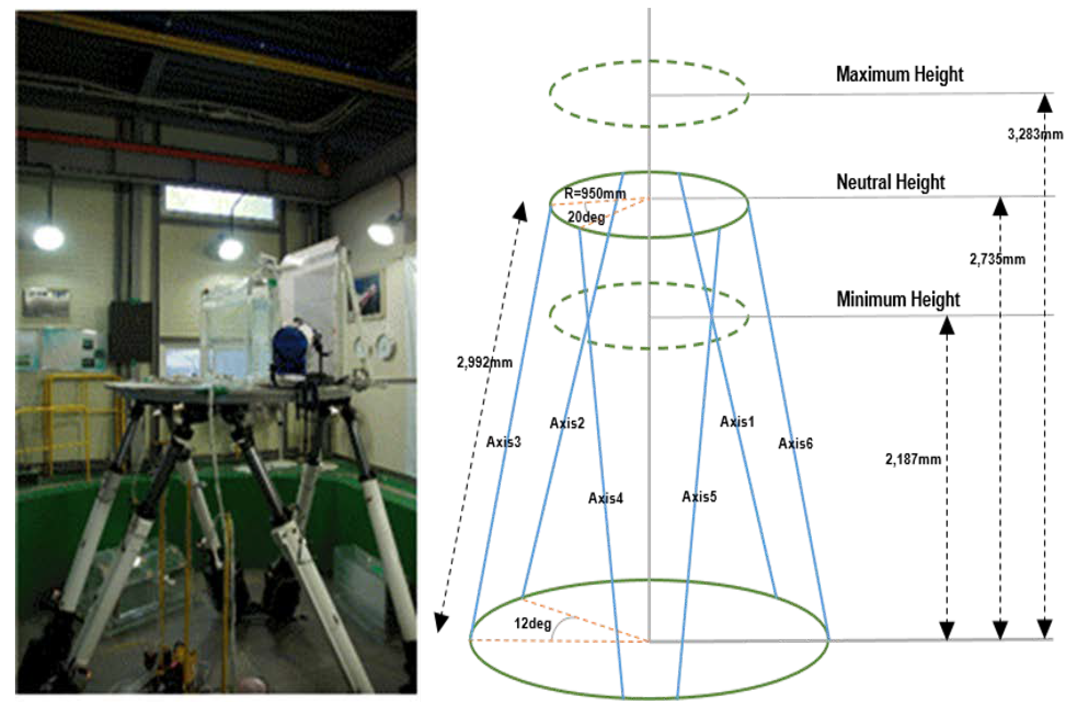
The sloshing motion platform (SMP) used in this study was a device capable of implementing six degrees of freedom using six actuators. The SMP was designed to bear dynamic loads 4000 kgf (approximately 39,230 N).
Figure 1 is a schematic of the model tank used in this experimental setup on the SMP and its specifications. When the servo motor mounted on the bottom of the SMP rotates, the six actuators are converted into sway motion via inner screws, which enable 6 degrees of freedom of movement. Table 1 and Table 2 list the mechanical specifications and maximum speeds of the actuator motion. The motion control system is divided into a system console unit, motion control unit, and motion control software. The system console unit transfers and controls the necessary input values. It consists of a host computer with digital signal processor, a signal board, and an interface control unit. The motion control unit consists of a digital signal processor/rotations per minute embedded motion control program, power supply, motion plate design/tuning/operation software, and an API library. To prevent a malfunction of the entire system, limit switches were also installed in each actuator.
2.2. Test Model
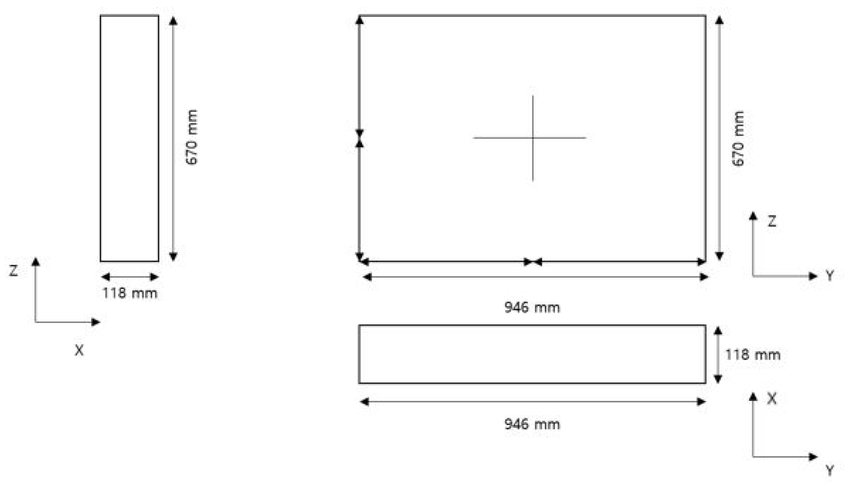
The model tank used in this study was a rectangular parallelepiped tank made of acrylic. The lower surface of the model tank was 946 mm × 118 mm and the height was 670 mm. Figure 2 shows the dimensions of the model tank made in our laboratory.
2.3. Pressure Sensor, Data Acquisition System, and Sensor Cluster
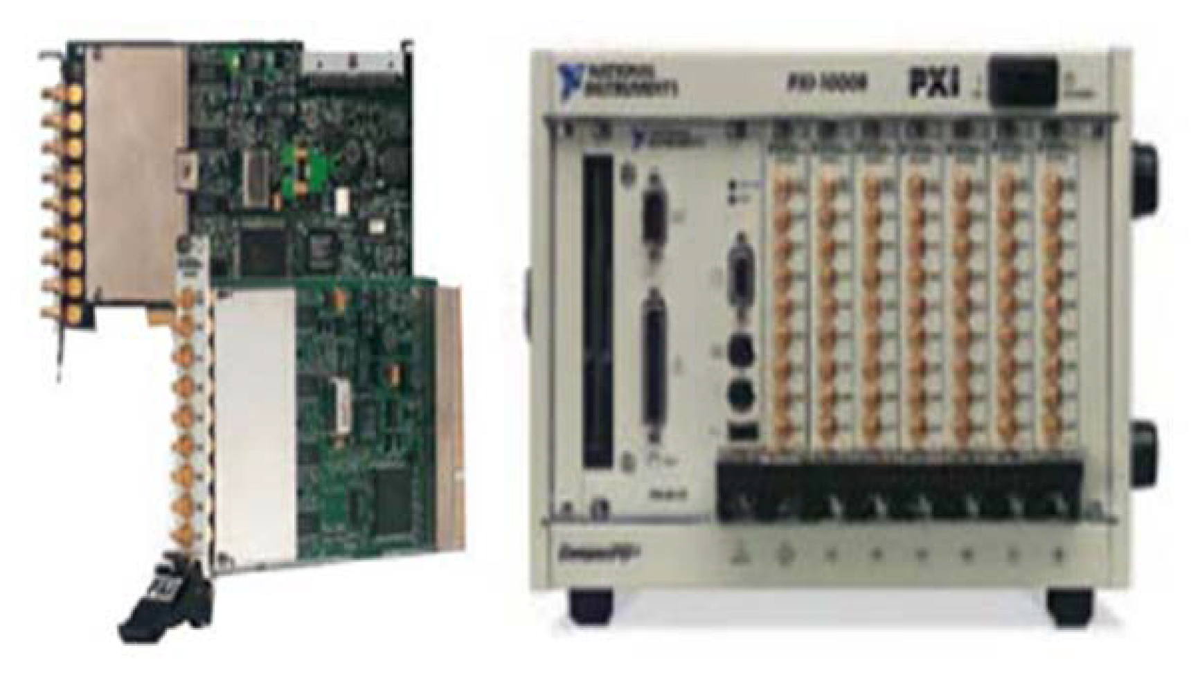
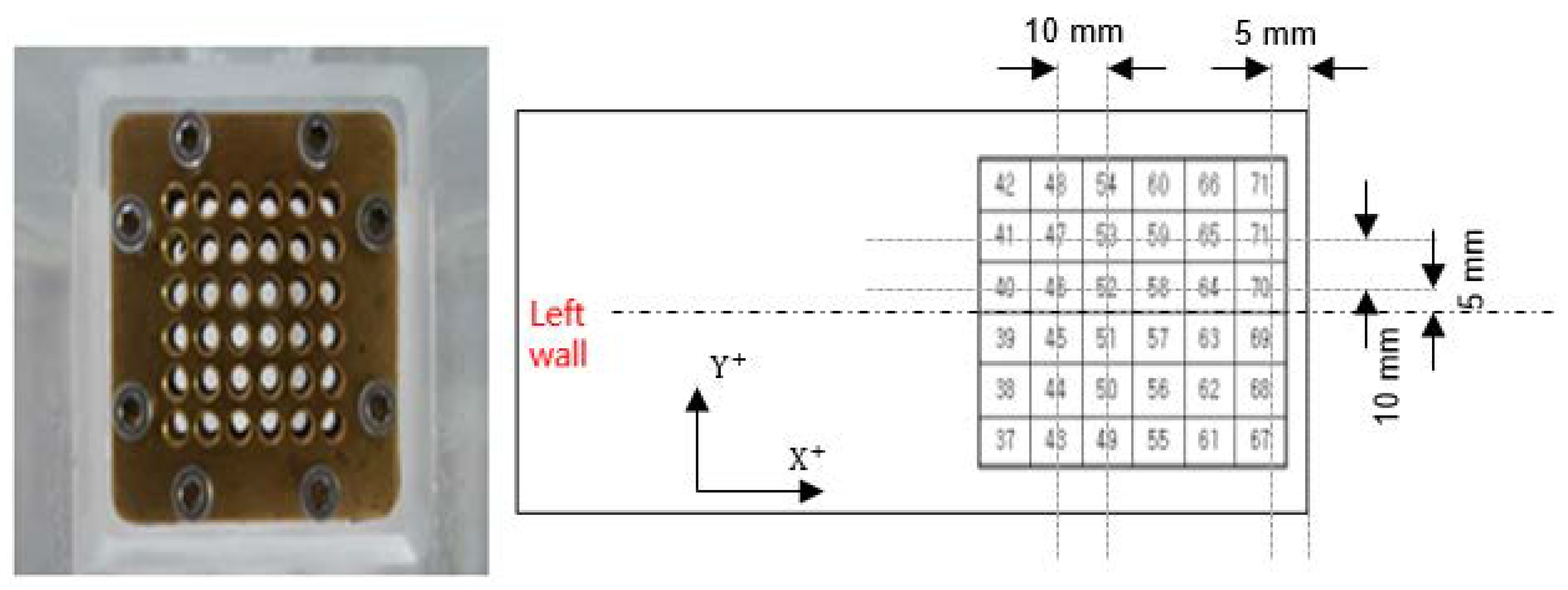
The data acquisition systems used in this experiment comprised a pressure gauge and data logger. Shown in Figure 3, the pressure gauge is a 211B5 integrated circuit piezoelectric (ICP) type from Kistler. The 211B5 is 5.5 mm in diameter and does not require other amplifiers. Details on the pressure gauge are listed in Table 3. Shown in Figure 4, the PXI-4472B board used to acquire data was purchased from National Instruments. This board has 24-bit resolution and can sample up to 102.4 kS/s with each channel. Details on the board are listed in Table 4. The cluster was made of brass and contained holes for the insertion of 36 sensors. In this experiment, the pressure was measured by attaching the sensors from Channel 36 to Channel 72 (Figure 5) on the upper surface of the model tank. Figure 5 shows the cluster and channel numbers of the sensors for each location.
2.4. Flow Visualization Device
2.5. Experimental Conditions
The experiments were conducted by dividing the test conditions into SWAY and ROLL excitation motions, both with the same filling level. The experiments were carried out with a single impact test irrespective of the test condition. For each condition, two sets of ten experiments. Table 6 shows the test condition details, and Table 7 lists the air and water temperature for each set, where 1 set is 10 tests. The temperature of the water and air was measured by two digital thermometer. The temperature in Table 7 is the mean temperatures of each set. The temperature of the water and measured by two digital thermometers. The temperature in Table 7 is the mean temperatures of each set. The variation of the temperature was less than 0.3 °C.
2.6. Peak Pressure Detection
The pressure data were measured at the thirty-six positions for each test and the peak pressure was defined as the maximum value among the pressure data. The threshold pressure is a specific value as noise level. In this test, the threshold pressure set to 0.02 bar was excluded. The time intervals between adjacent maximum pressures were checked. The time interval was set to a one-half period, which corresponded to the maximum value of the spectrum amplitude from fast Fourier transform (FFT) results. Figure 7 shows the peak acquisition algorithm used in this experiment. The offset correction of the signals was done twice. One was done before measuring the data using the data-acquisition software. The other was done during the post-data process using the data recorded for 10 s before the test.
3. Results and Discussion
3.1. Flow Visualization
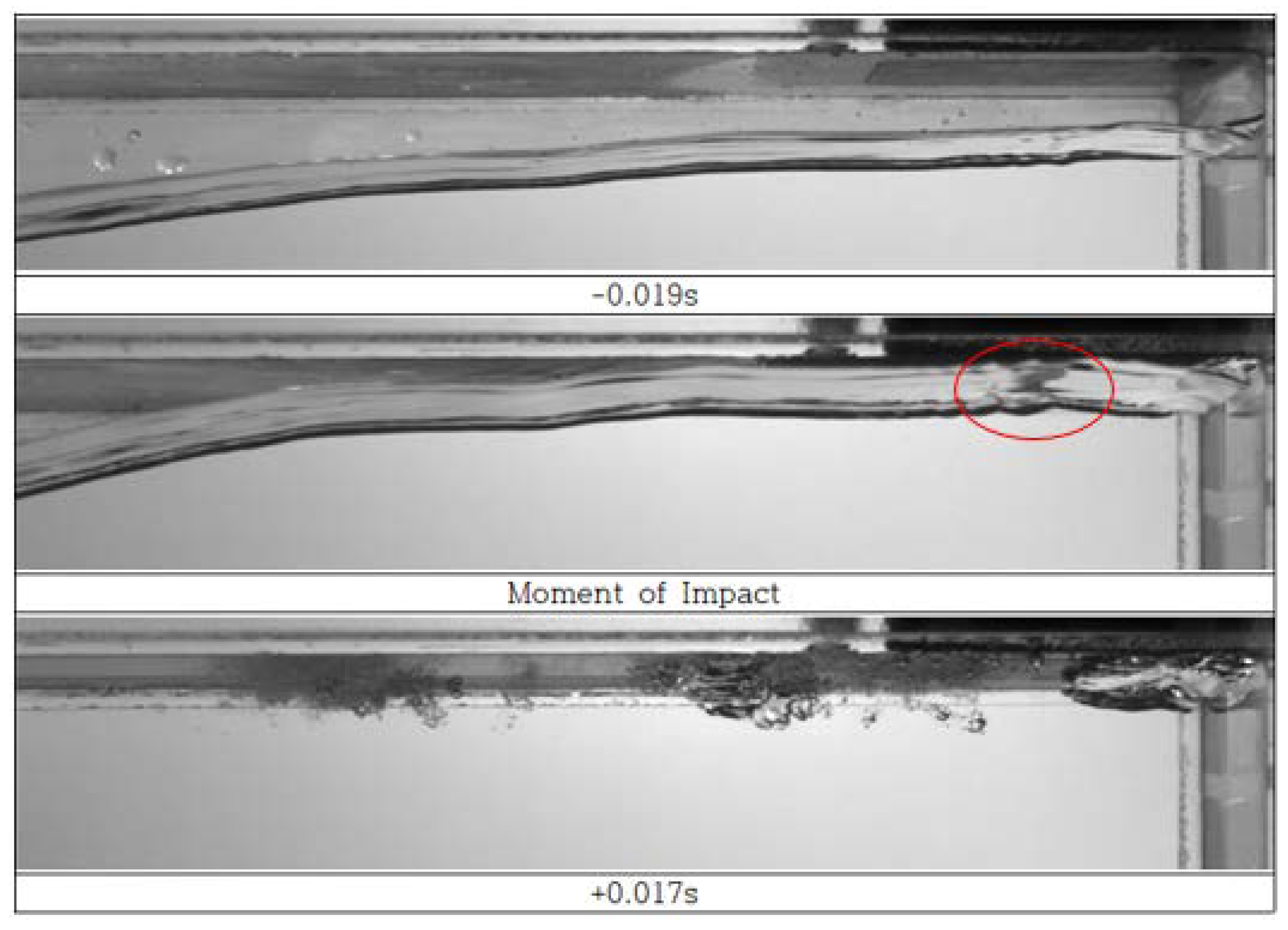
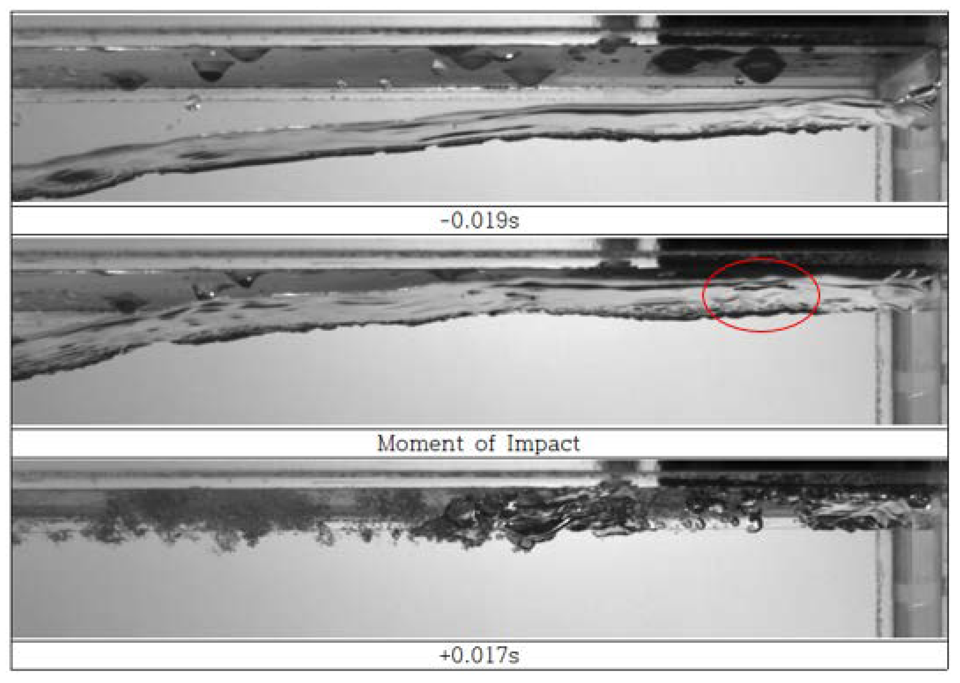
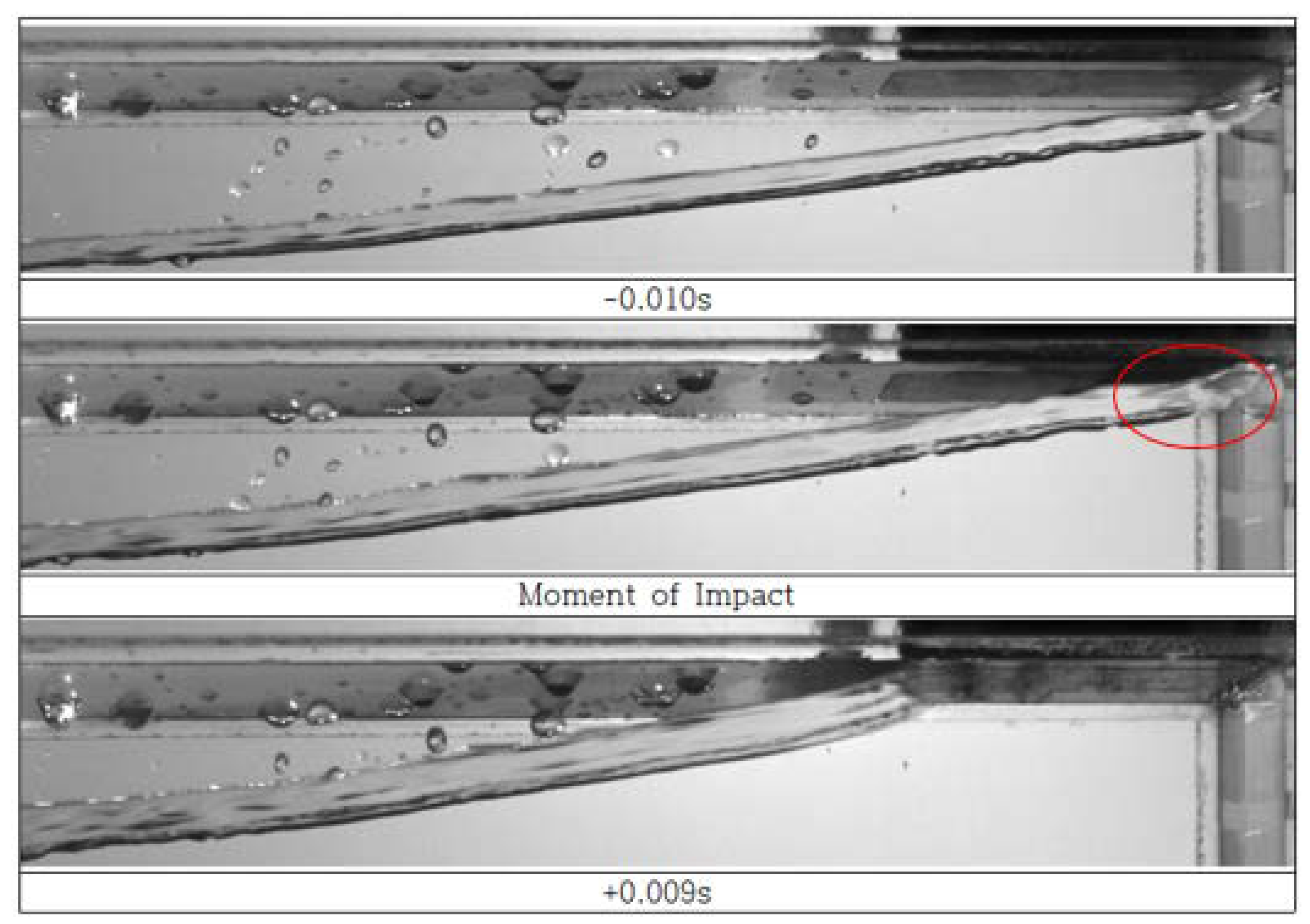
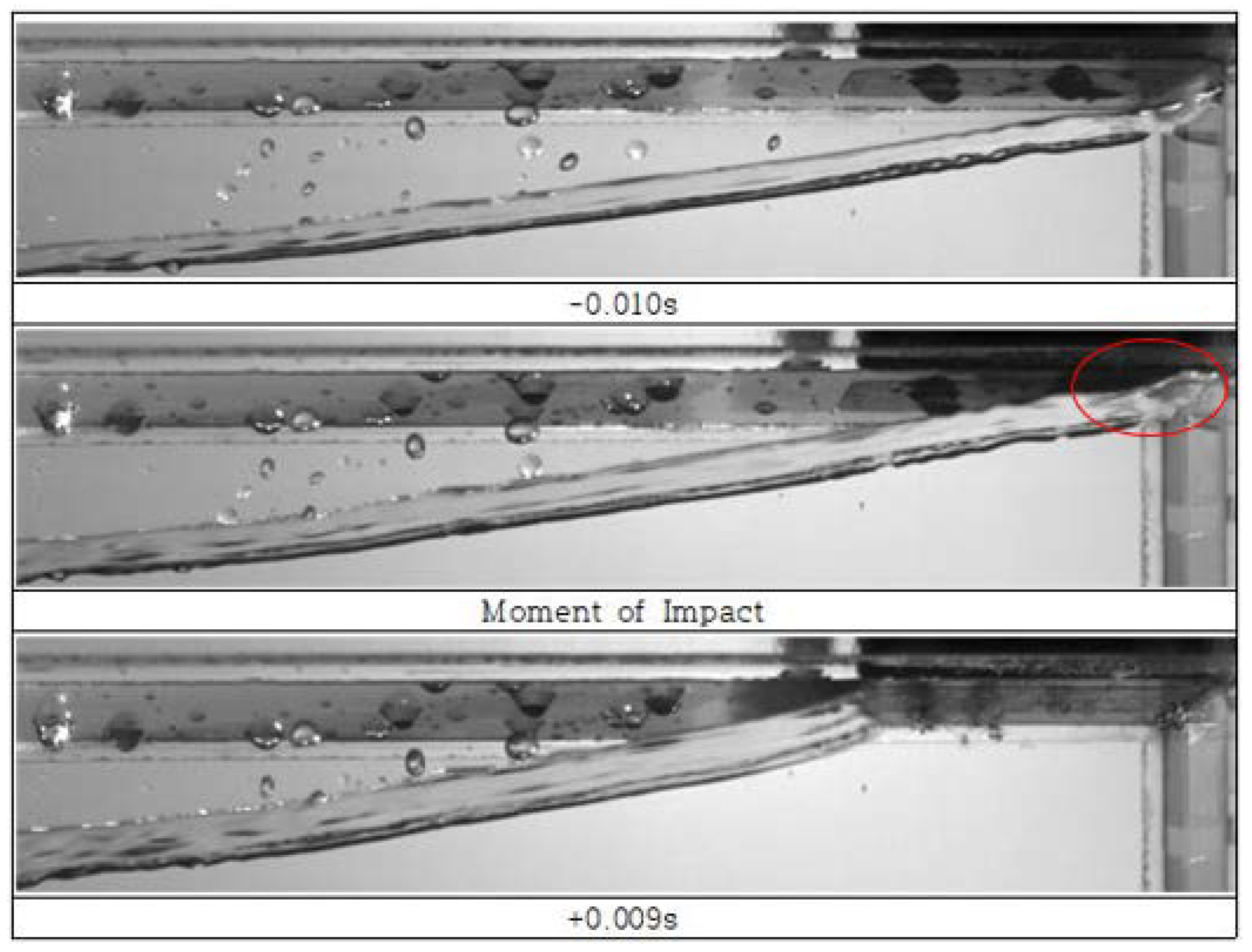
Between the 20 repeated experiments, the macroscopic flow was very similar. However, there were differences in the microscopic flow between individual experiments. For SWAY and ROLL, the sensor surface conditions were divided into wet and dry conditions depending on the presence of water on the sensor surface. Figure 8, Figure 9, Figure 10 and Figure 11 are the macroscopic flow snapshots of the wet and dry conditions. Close snapshots before and after the first impact are shown in Figure 12, Figure 13, Figure 14 and Figure 15. In both SWAY and ROLL, the macroscopic flows were similar regardless of the wet or dry condition. However, Figure 8, Figure 9, Figure 10 and Figure 11 show that there were differences in the microscopic flow around the sensor cluster after the initial impact for certain test conditions.
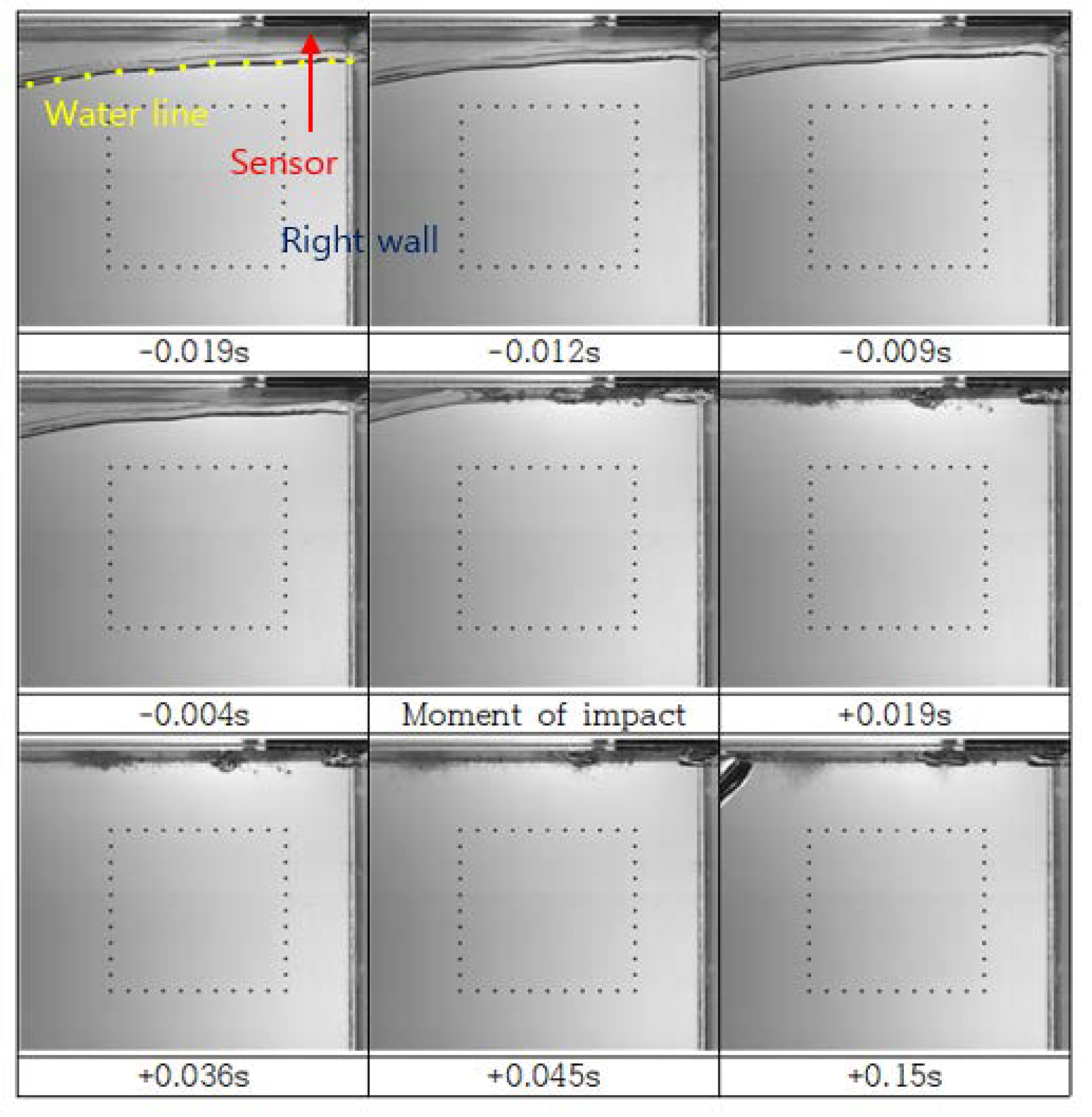
Referring to the position of sensors shown in Figure 5, for SWAY, the sensors at Channels 36–60 measured the impact pressure directly via water contact. On the other hand, the Channels 61–72 sensors measured the impact pressure via air pockets under the sensor cluster. This was further investigated by analysis of the snapshots. In the dry condition, bubbles were hardly generated after the impact, as shown in Figure 12. In the wet condition, bubbles were generated around locations where droplets formed, as shown in Figure 13.
3.2. Microscopic Flow Comparison
Regardless of the wet or dry condition, the overall trends of the average peak pressure values for all channels were very similar between SWAY and ROLL. The peak pressures measured from the 20 repeated experiments had large variations between experiments, even in the same channel, which was thought to be caused by the differences in microscopic flows.
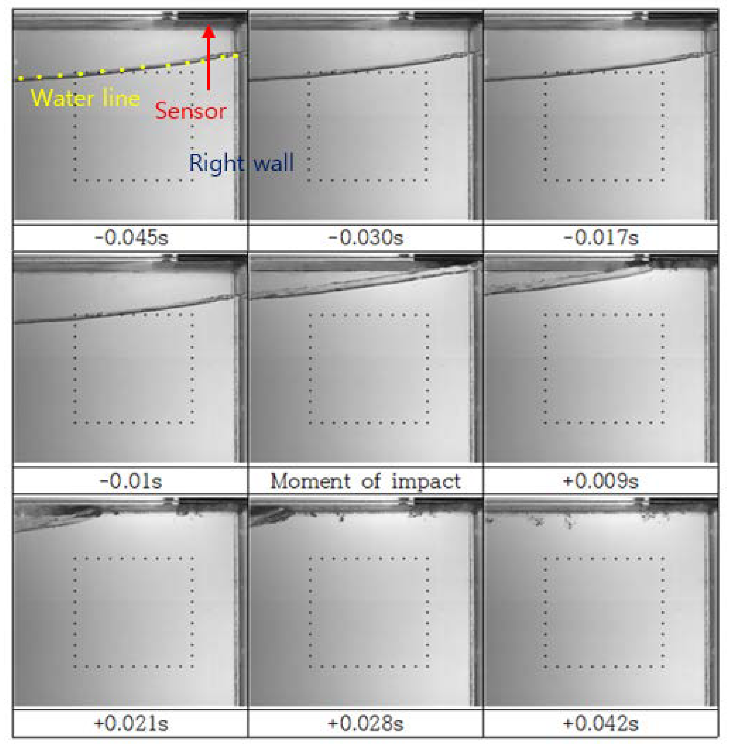
Figure 16 and Figure 17 are 10 time-series pressure graphs randomly derived from four channels around a center line of the sensor cluster array for the wet condition in SWAY and ROLL. For the sway motion, the water surface touched the ceiling first and, then moved to the right wall, which resulted in a big air pocket between the water surface and the ceiling as shown in Figure 12 and Figure 13. The trapped air pocket collapsed into small bubbles and this collapse caused the strong oscillation with the high-frequency in the impact pressure signals as shown in Figure 16. For the roll motion, the air pocket was not trapped because the water surface touched the right wall first and then swept the ceiling as shown in Figure 14 and Figure 15. The oscillation in the impact pressure signal in Figure 17 was substantially smaller compared to the sway motion. The smaller oscillation was caused by the collision of the droplets. The collision direction between the droplets and the wave surface induced a difference in the number of bubbles generated. Generally, more bubbles are generated when the water surface collides with the droplet at s smaller angle than the right angle [25,26,27,28].
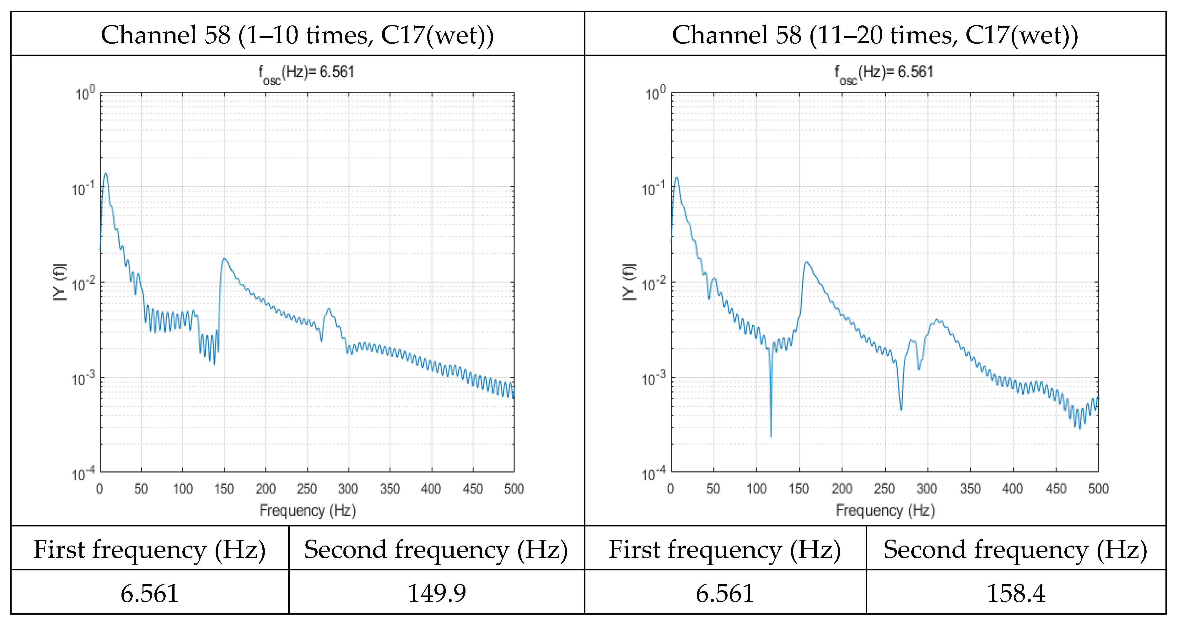
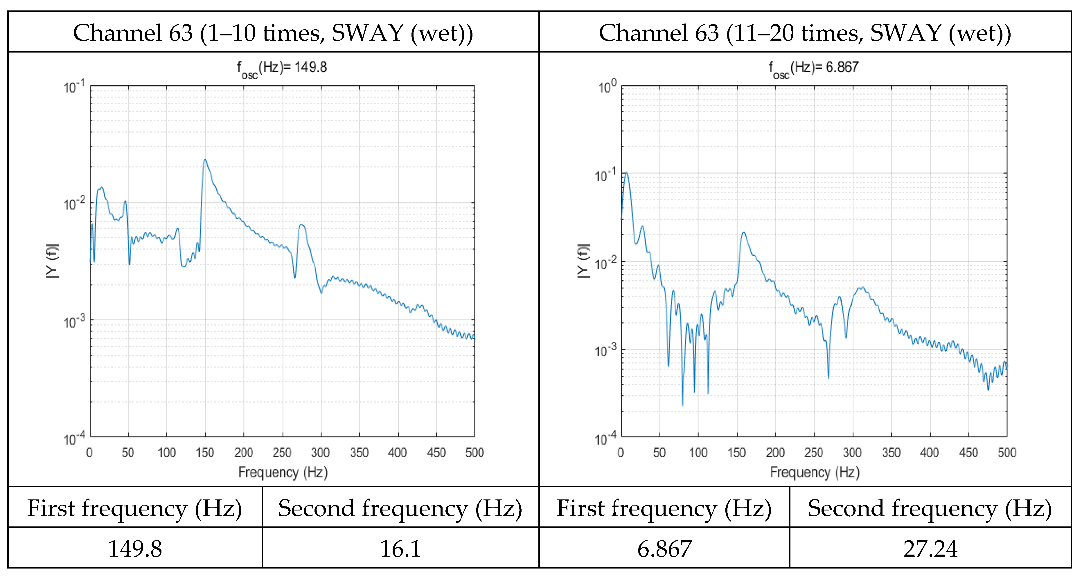
For the SWAY, where bubbles were abundantly generated, high-frequency oscillation occurred as shown in Figure 16. Figure 18, Figure 19, Figure 20 and Figure 21 show the results of a FFT frequency analysis of the data in Figure 16. The FFT analysis was performed twice by dividing the 20 total runs of experimental data into 10 each depending on the experimental temperature. Both FFT results showed a first peak caused by a major impact at 6–7 Hz and a second peak at 150–160 Hz. This result was judged to arise from air pockets observed in the flow visualization and from the oscillation of the many bubbles produced immediately after the impact. The distribution of local pressure was determined to be significantly different depending on the experiments because of the different microscopic flow behaviors.
3.3. Factors Affecting Peak Pressure Measurements
3.3.1. Peak Pressure Results of Two Sensor’s Surface Conditions
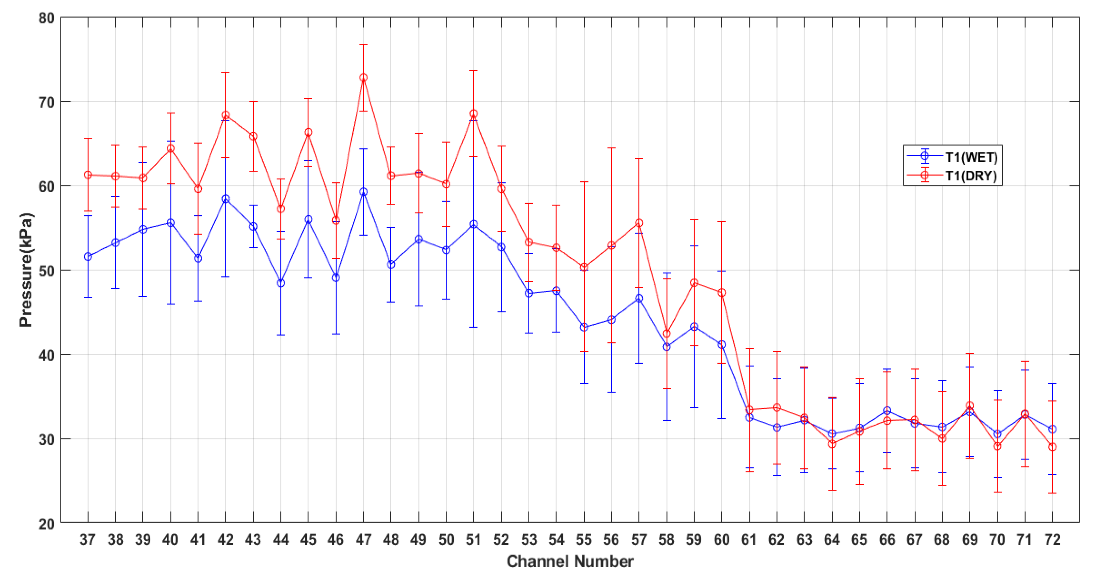
For each motion, two sets of ten experiments were conducted. The average of the first impact peak pressures and standard deviations measured at each channel are shown in Figure 22 and Figure 23. Figure 22 is a comparison of SWAY wet and dry condition average peak pressures. The average of the first impact peak pressures measured in the dry condition increased significantly from the Channel 37 to the Channel 60 sensors, which were located in the sensor cluster. The channel number from 37 to 60 corresponded to impact zone which the water collides directly. The Channel 47 sensor had the largest difference of approximately 13.5 kPa. For the Channel 61 to Channel 72 sensors, where water did not make direct contact (simply get wet), the average pressures were almost identical in both the wet and dry conditions.
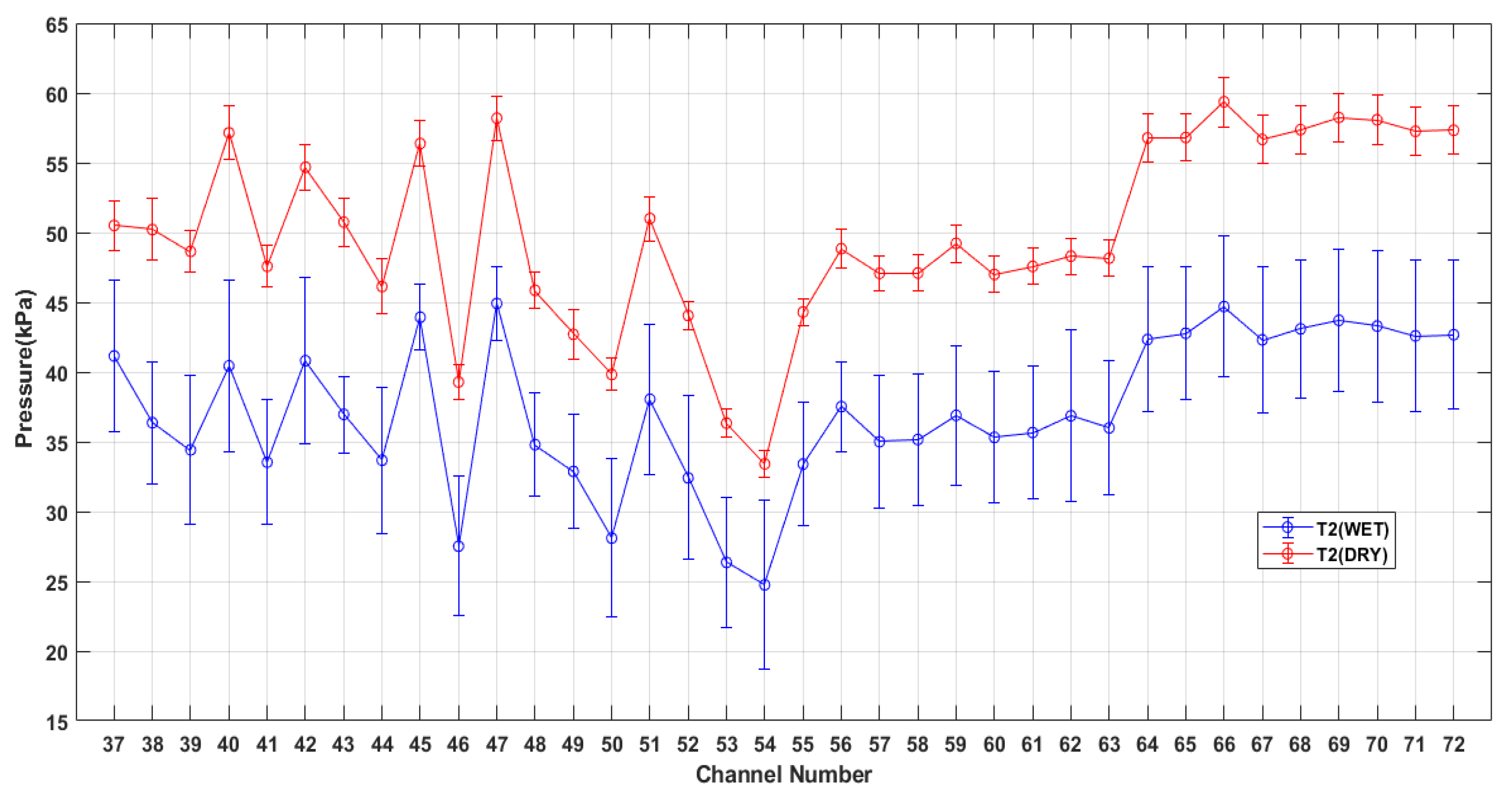
Figure 23 is a comparison of ROLL wet and dry condition average peak pressures. For ROLL, water directly contacted the entire sensor cluster, and the average pressure in all channels increased significantly compared to the wet condition. The Channel 40 sensor had the largest difference of approximately 18.3 kPa. The graphed trends between wet and dry conditions were very similar between SWAY and ROLL. For the wet condition, however, there was a difference in sensor peak pressure where water came into direct contact as compared to the dry condition. Due to the microscopic flow differences, the wet condition showed larger deviations than dry in the same repeated experiments.
3.3.2. Effect of Thermal Shocks
The Kistler 211B5 sensor used in this experiment was an ICP type, and thus it was highly influenced by the difference in temperature between the sensor and the medium [22,23,24]. Pistani and Thiagarajan [22] found that the pressure signal changed when the dry sensor touched the water. They showed that a positive pressure signal occurred when the water temperature was lower than the air temperature, and a negative pressure signal occurred when the water temperature was higher than the air temperature.
In this experiment, the effect of thermal shock was also investigated by analyzing the difference between pressures measured in the wet and dry conditions. The sensor temperatures were set to match the air temperature for each experiment in the dry condition. On the other hand, the sensor temperatures in the wet condition were set to an average between the air and water temperatures since the sensor cluster was not completely wet in Figure 13 and Figure 15. Details on the air and water temperatures are given in Table 7. For SWAY, a thermal shock effect was observed in the sensors from Channel 37 to Channel 60 where water made direct contact. The average difference between the sensor and water temperatures was 2.1 °C for the dry condition and 0.9 °C for the wet condition. In both the wet and dry conditions, positive thermal shock effects occurred because the sensor temperatures were higher than that of the medium. For the dry condition, where the temperature difference was larger compared to the wet condition, a larger thermal shock effect occurred, and the pressure difference reached 13.5 kPa (22.5%).
The thermal shock effect did not occur in sensors Channel 61–72, where peak pressures were measured via air pockets formed under the sensor cluster. For ROLL, where the peak pressure was measured through direct contact with water on all sensors, a thermal shock effect occurred on all channels. The temperature difference between the sensor and the water in the dry condition of ROLL was very small, 0.05 °C on average, and 2.7 °C on average in the wet condition.
For the dry condition, a thermal shock effect did not occur because there was no temperature difference between the sensor and medium. On the other hand, for the wet, a negative thermal shock effect occurred because the sensor temperature was lower than that of the medium. As the result, a pressure difference of up to 18.3 kPa (31.4%) occurred in the dry condition compared to the wet.
3.3.3. Effects of Droplets on the Sensor Surfaces
Directly formed droplets were observed in wet conditions experiments. Experimental cases with distinct droplet locations and sizes (the second SWAY test and tenth ROLL test) to determine whether these properties also affected the peak pressures. For the second SWAY test, droplets formed near Channel 37, Channel 47, and Channel 57, as shown in Figure 24. For the tenth ROLL test, droplets formed near Channel 47 and Channel 56, as shown in Figure 25. Figure 26 and Figure 27 show the average peak pressures from 20 runs of the dry condition (red solid line) and wet condition (blue solid line) and the measured peak pressures of the selected SWAY and ROLL cases. The locations of droplets are selectively depicted with red circles and the locations of near droplets are depicted with orange circles. Standard deviations are expressed using error bars.
For the second SWAY test, the peak pressures measured at the Channel 37, Channel 47, and Channel 57 sensors showed different trends between wet and dry conditions, as shown in Figure 26. At the Channel 37 sensor, the average peak pressure difference over 20 runs for the dry was 29.94% and for the wet was 16.74%. At the Channel 47 sensor, the difference for the dry was 40.07% and for the wet was 26.34%. At the Channel 57 sensor, the differences were 35.35% and 22.99% for dry and wet, respectively. When the peak pressures were compared to the wet condition, the measurement errors in the dry condition increased by 78% due to the thermal shock.
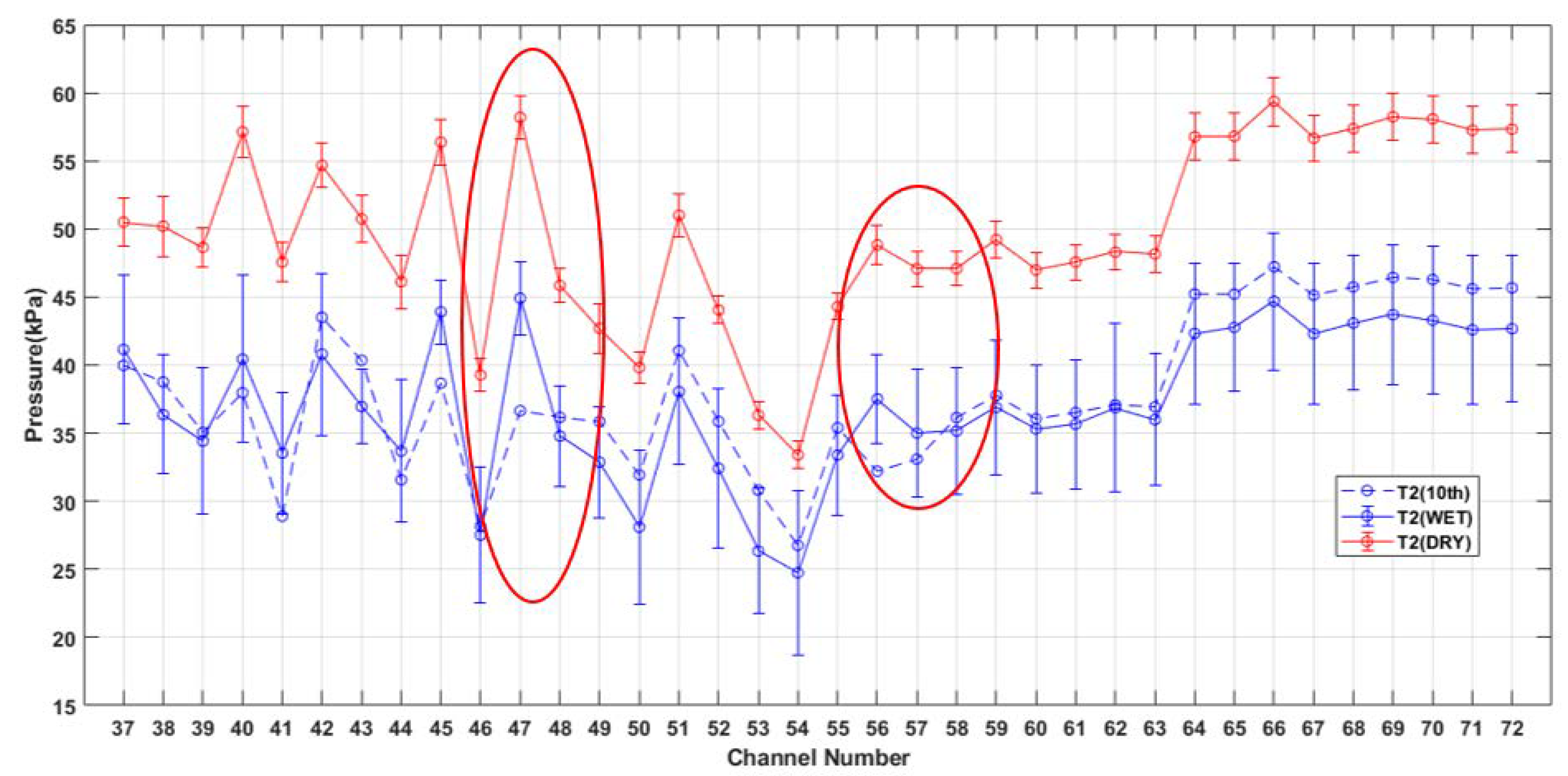
For the 10th ROLL test, the peak pressures measured at the Channel 47 and Channel 56 sensors showed different trends between wet and dry conditions, as shown in Figure 27. At the Channel 47 sensor, the average peak pressure difference over 20 runs for the dry was 37.03% and for the wet was 18.39%. At the Channel 56 sensor, the difference for the dry was 34.05% and for the wet was 14.15%. Furthermore, the pressures of the corresponding sensors in the SWAY and ROLL experiments were outside the error bars of the average pressures for each wet condition, as shown in Figure 26 and Figure 27. Peak pressure details for SWAY and ROLL are summarized in Table 8.
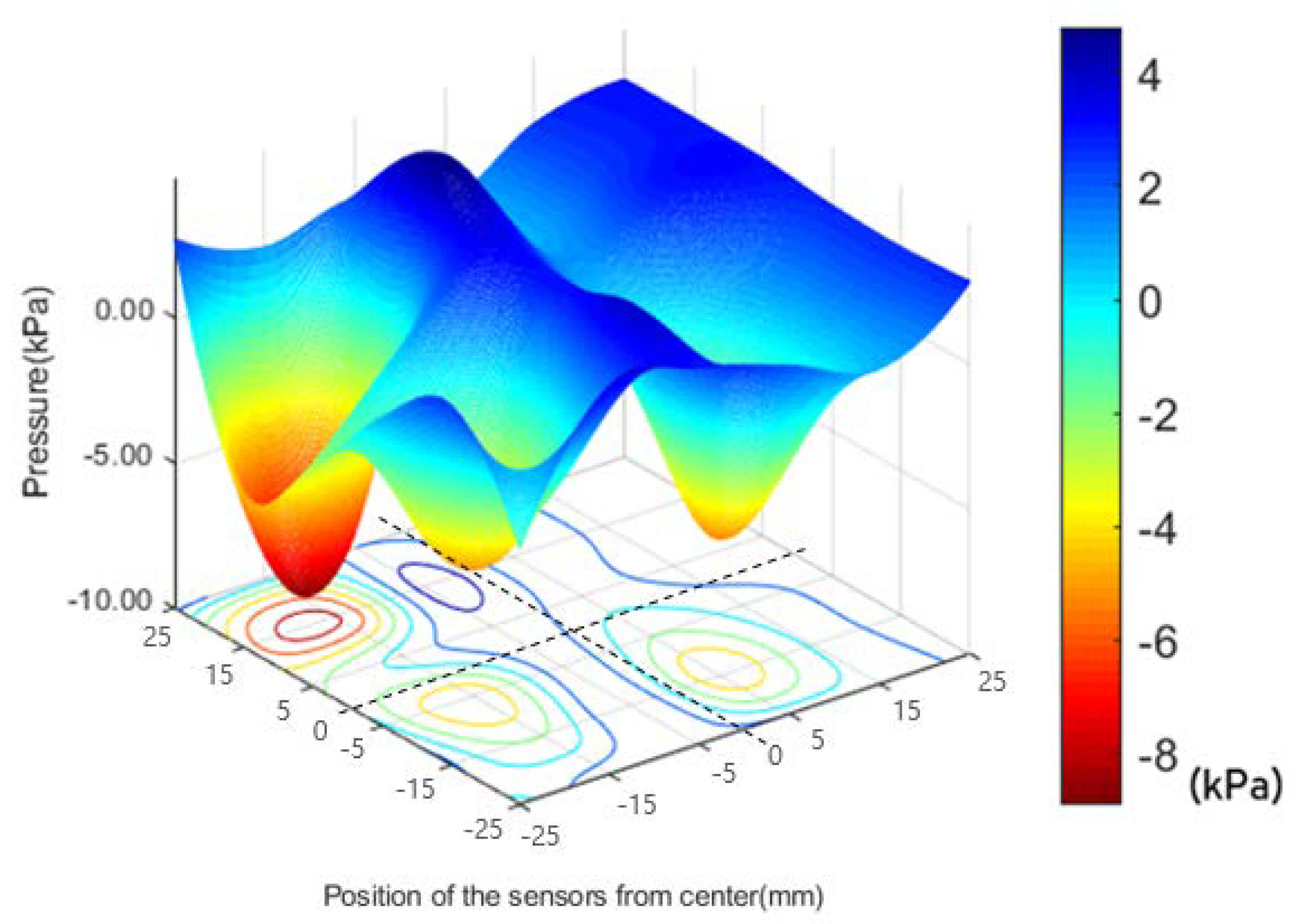
Figure 28 and Figure 29 are 3D plots of peak pressure differences for the selected cases and wet conditions for each test. For continuity, the grids of the graphs were constructed with 40 divisions between the sensors, and the measured peak pressures were interpolated using cubic spline curves for continuity. In SWAY, the peak pressure differences were high at Channel 37, Channel 47, and Channel 57 where the droplets had formed, as shown in Figure 28. Likewise, the pressure differences were high at Channel 47 and Channel 56 in ROLL, as shown in Figure 29.
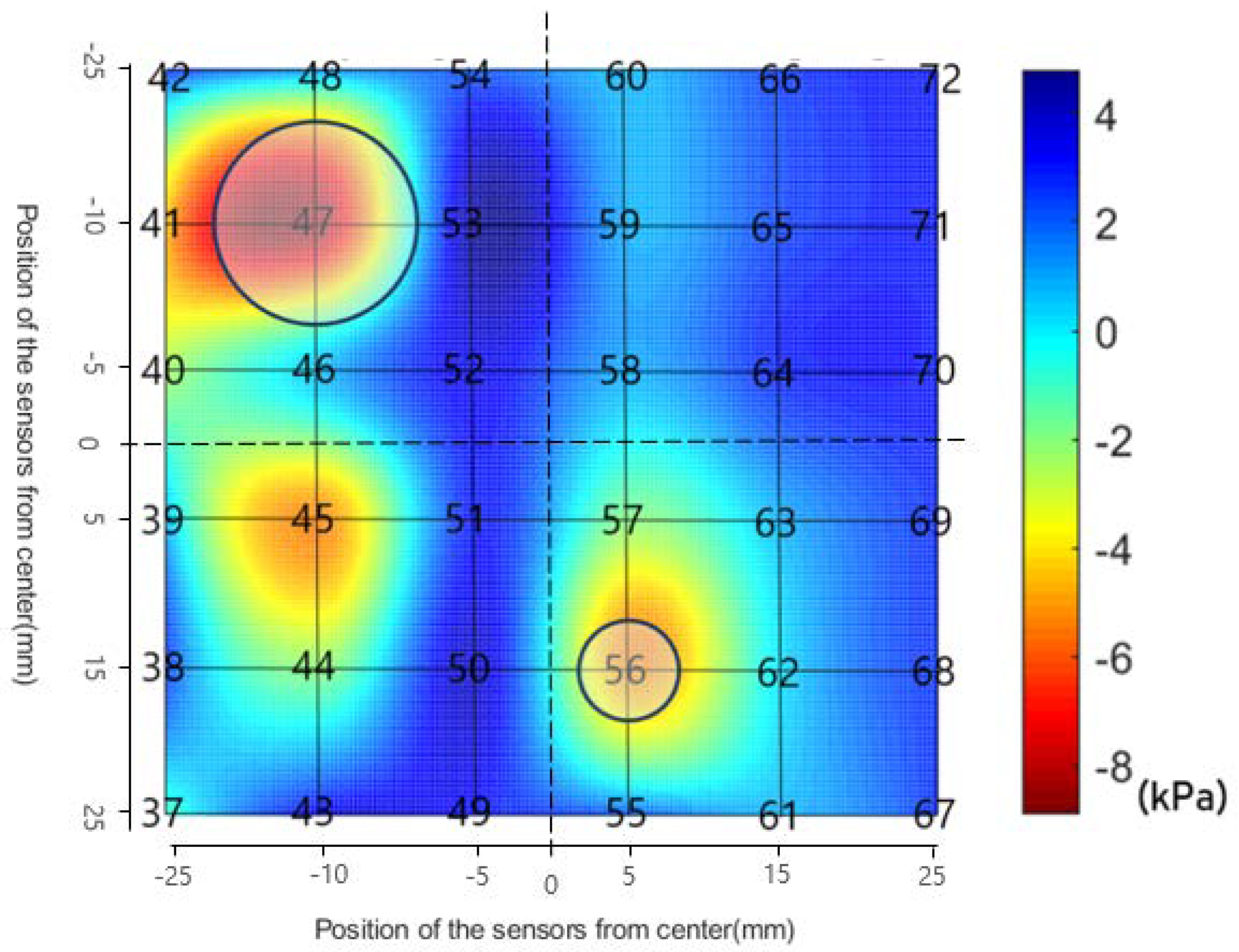
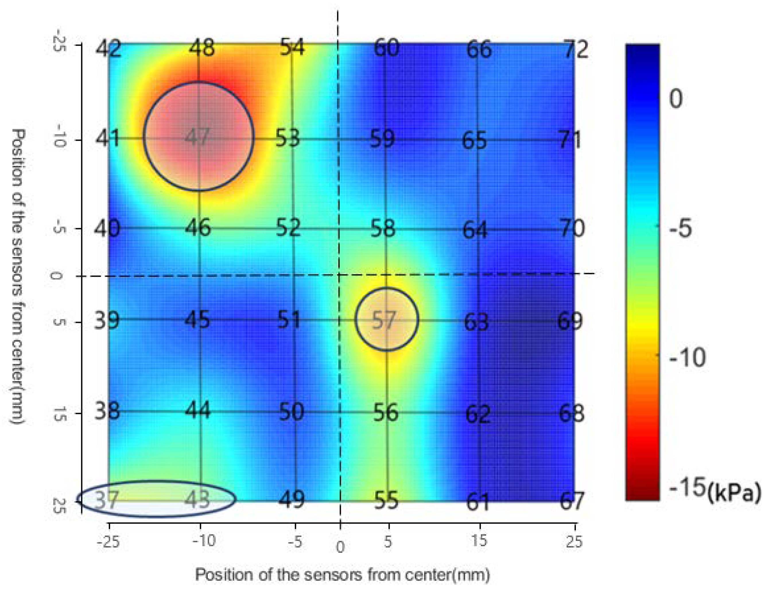
Figure 30 and Figure 31 are contours of the results from Figure 28 and Figure 29 considering the locations of the sensors. Droplet locations are marked with circles on the graphs. The reason why the pressure of the sensors with droplets differed from the wet condition average was related to droplet movement upon impact. This droplet movement arose from surface tension differences caused by dissimilar contact angles between the wave’s surface and the droplets. The differences in surface tension caused droplets with large contact angles to move to the wave surface with a low angle [29]. Upon impact, the droplets on the sensor came in contact with the wave surface and collided with the rising wave surface particles. The collision reduced the kinetic energy of the particles approaching the sensor, therefore reducing the dynamic pressure.
The viscosity and surface tension that are changed by the temperature of the water and the scale of the model tank affect the change instability of the free water surface and the profile of the flow velocity. These can cause the different sloshing impact load. In this research, the water temperature was at 11.2 °C~12.8 °C and the viscosity and surface tension were not affected significantly by the variation of the temperature. The influences of the scale of the model tank on the instability of the free water surface and the profile of the flow velocity should be investigated further in the future.
4. Conclusions
Based on the experimental results of this study, the following conclusions were obtained. More bubbles were generated on the sensor cluster in the wet condition than in the dry condition for both SWAY and ROLL upon impact. In the SWAY case, more bubbles were generated than in ROLL because of the difference in angles between the free surface and the droplets upon impact.
- (1)
- The high-frequency oscillation caused by the bubbles was more prominent in SWAY than in ROLL. The amount of bubbles depended on the direction of the wave surface. For the sway motion, the water surface touched the ceiling first and, then moved to the right wall, which resulted in a big air pocket. The strong oscillation with the high frequency in the impact pressure signals was caused by the collapse of the trapped air pocket in to the bubbles. The strong oscillations were in the rage of approximately 41.6%~54.5% of the maximum peak pressure.
- (2)
- The ICP sensors used in the measurement of the sloshing impact were sensitive to differences in the temperature between the air and water. The difference in the temperature of the two mediums causes the error in the measurement of the impact pressure, which is called the thermal shock. In this research, the thermal shock resulted in the measurement errors of about 10% to 31.4%. These errors can be minimized by making the temperature of the water and air equal.
- (3)
- In the wet condition, water droplets located directly on the sensor cluster affected the measurement in the impact pressures, as well. The droplet on the sensor is absorbed into the water surface upon impact, which reduces the kinetic energy of water particles approaching the sensor. This phenomenon reduces the dynamic impact pressure. When the water droplets were formed on the sensor, the impact pressure was measured to be approximately 14% to 26% lower than when the water droplets were not formed in the wet condition. When the peak pressures were compared to the dry condition, the measurement errors increased to approximately 30% to 40% due to the thermal shock.
Errors related to sensors in sloshing impact tests were investigated in this study, and the causes of the errors were analyzed. More studies and analyses are required to fundamentally understand the sloshing impact load test and to reduce test errors.
Author Contributions
D.H.K and E.S.K.- experiments, data analysis, original draft preparation, and review and editing, S.-c.S. and S.H.K.-methodology, supervision, and original draft preparation, The final manuscript has been approved by all the authors.
Funding
This research was funded by the National Research Foundation of Korea(NRF) grant funded by the Korea government(MSIT) through GCRC-SOP (No. 2011-0030013).
Conflicts of Interest
The authors declare no conflict of interest.
References
- Shin, Y.Y.; Kim, J.W.W.; Lee, H.H.; Hwang, C. Sloshing Impact of LNG Cargoes in Membrane Containment Systems in the Partially Filled Condition. In Proceedings of the Thirteenth International Society of Offshore and Polar Engineering Conference, Honolulu, HI, USA, 25–30 May 2003. ISOPE-I-03-274. [Google Scholar]
- Souto-Iglesias, A.A.; Delorme, L.L.; Pérez-Rojas, L.; Abril-Pérez, S. Liquid moment amplitude assessment in sloshing type problems with smooth particle hydrodynamics. Ocean Eng. 2006, 33, 1462–1484. [Google Scholar] [CrossRef]
- Idelsohn, S.; Marti, J.; Souto-Iglesias, A.; Oñate, E. Interaction between an elastic structure and free-surface flows: Experimental versus numerical comparisons using the PFEM. Comput. Mech. 2008, 43, 125–132. [Google Scholar] [CrossRef]
- Khayyer, A.; Gotoh, H. Wave impact pressure calculations by improved SPH methods. Int. J. Offshore Polar Eng. 2009, 19, 300–307. [Google Scholar]
- Bulian, G.; Souto-Iglesias, A.; Delorme, L.; Botia-Vera, E. Smoothed particle hydrodynamics (SPH) simulation of a tuned liquid damper (TLD) with angular motion. J. Hydraul. Res 2010, 48, 28–39. [Google Scholar] [CrossRef]
- Degroote, J.; Souto-Iglesias, A.; Paepegem, W.V.; Annerel, S.; Bruggeman, P.; Vierendeels, J. Partitioned simulation of the interaction between an elastic structure and free surface flow. Comput. Methods Appl. Mech. Eng. 2010, 199, 2085–2098. [Google Scholar] [CrossRef] [Green Version]
- Loysel, T.; Chollet, S.; Gervaise, E.; Brosset, L.; De Seze, P.E. Results of the First Sloshing Model Test Benchmark. In Proceedings of the Twenty Second International Society of Offshore and Polar Engineering Conference, Rhodes, Greece, 17–22 June 2012. ISOPE-I-12-370. [Google Scholar]
- ABS. Strength Assessment of Membrane-Type LNG Containment Systems Under Sloshing Loads; American Bureau of Shipping: Houston, TX, USA, 2006; pp. 1–79. [Google Scholar]
- DNV. Sloshing Analysis of LNG Membrane Tanks; Det Norske Veritas: Hovik, Norway, 2006; pp. 1–49. [Google Scholar]
- BV. Sign Sloshing Loads for LNG Membrane Tanks; Bureau Veritas: Paris, France, 2011; pp. 1–37. [Google Scholar]
- Kuo, J.F.; Campbell, R.B.; Ding, Z.; Hoie, S.M.; Rinehart, A.J.; Sandström, R.E.; Yung, T.W.; Greer, M.N.; Danaczko, M.A. LNG Tank Sloshing Assessment Methodology–The New Generation. In Proceedings of the Nineteenth International Society of Offshore and Polar Engineering Conference, Osaka, Japan, 21–26 July 2009. ISOPE-I-09-062. [Google Scholar]
- Lugni, C.; Brocchini, M.; Faltinsen, O.M. Wave impact loads: The role of the flip-through. Phys. Fluids 2006, 18, 122101. [Google Scholar] [CrossRef]
- He, H.; Kuo, J.F.; Rinehart, A.J.; Yung, T.W. Influence of Raised Invar Edges on Sloshing Impact Pressures. In Proceedings of the Nineteenth International Society of Offshore and Polar Engineering Conference, Osaka, Japan, 21–26 July 2009. ISOPE-I-09-065. [Google Scholar]
- Yung, T.W.; Ding, Z.; He, H.; Sandström, R.E. LNG sloshing: Characteristics and scaling laws. Int. J. Offshore Polar Eng. 2009, 19, 264–270. [Google Scholar]
- Maillard, S.; Brosse, L. Influence of Density Ratio between Liquid and Gas on Sloshing Model Test Results. In Proceedings of the Nineteenth International Society of Offshore and Polar Engineering Conference, Osaka, Japan, 21–26 July 2009. ISOPE-I-09-043. [Google Scholar]
- Malenica, S.; Kwon, S.H. An overview of the hydro-structure interactions during sloshing impact of tanks of LNG carriers. Brodogradnja/Shipbuilding 2013, 4, 22–30. [Google Scholar]
- Yang, Y.J.; Kwon, S.H.; Park, S.G.; Lee, S.B.; Park, J.S. Remote sensing of wave directionality by two-dimensional directional wavelets: Part 2. Applications to the numerical and field data. Brodogradnja/Shipbuilding 2014, 65, 1–13. [Google Scholar]
- Kim, S.Y.; Kim, Y.; Park, J.J.; Kim, B. Experimental study of sloshing load on LNG tanks for unrestricted filling operation. J. Adv. Res. Ocean Eng. 2017, 3, 41–52. [Google Scholar] [CrossRef]
- Kaminski, M.L.; Bogaert, H. Full Scale Sloshing Impact Tests. In Proceedings of the Nineteenth International Society of Offshore and Polar Engineering Conference, Osaka, Japan, 21–26 July 2009. ISOPE-I-09-036. [Google Scholar]
- Brosset, L.; Mravak, Z.; Kaminski, M.; Collins, S.; Finnigan, T. Overview of Sloshel Project. In Proceedings of the Nineteenth International Society of Offshore and Polar Engineering Conference, Osaka, Japan, 21–26 July 2009. ISOPE-I-09-037. [Google Scholar]
- Souto-Iglesias, A.; Botia-Vera, E.; Martin, A.; Perez-Arribas, F. A set of canonical problems in sloshing. Part 0: Experimental setup and data processing. Ocean Eng. 2011, 38, 1823–1830. [Google Scholar] [CrossRef] [Green Version]
- Pistani, F.; Thiagarajan, K. Experimental measurements and data analysis of the impact pressures in a sloshing experiment. Ocean Eng. 2012, 52, 60–74. [Google Scholar] [CrossRef]
- Choi, H.I.; Choi, Y.M.; Kim, H.Y.; Kwon, S.H.; Park, J.S.; Lee, K.H. A Study on the Characteristic of Piezoelectric Sensor in Sloshing Experiment. In Proceedings of the Twentieth International Society of Offshore and Polar Engineering Conference, Beijing, China, 20–25 June 2010. ISOPE-I-10-665. [Google Scholar]
- Kim, S.Y.; Kim, K.H.; Kim, Y. Comparative study on pressure sensors for sloshing experiment. Ocean Eng. 2015, 94, 199–212. [Google Scholar] [CrossRef]
- Bhaga, D.; Weber, M.E. Bubbles is ciscous liquids: Shapes, wakes and velocities. J. Fluid Mech. 1981, 105, 61–85. [Google Scholar] [CrossRef]
- Davis, R.M.; Talyor, F.R.S.; Geoffey, S. The Mechanics of rising bubbles. Proc. R. Soc. 1950, A200, 209–220. [Google Scholar]
- Florschuetz, L.W.; Chao, B.T. On the mechanism of vapor bubble collapse. J. Heat Transf. Trans. ASME 1965, 87, 209–220. [Google Scholar] [CrossRef]
- Grace, J.R.; Wairegl, T.; Nguyen, T.H. Shapes and velocities of single drops and bubbles moving freely through immiscible liquids. Chem. Eng. Res. Des. 1976, 54, 167. [Google Scholar]
- Nowak, M.; Xie, Z.; Kovalchuk, N.M.; Matar, O.K.; Simmons, M.J.H. Bulk advection and interfacial flows in the binary-coalescence of surfactant-laden and surfactant-free drops. Soft Matter 2017, 13, 4616–4628. [Google Scholar] [CrossRef] [PubMed]
Figure 1.
6-Degree of Freedom (DOF) Sloshing Motion Platform.

Figure 2.
Model tank dimensions.

Figure 3.
Photo of Pressure Sensor.
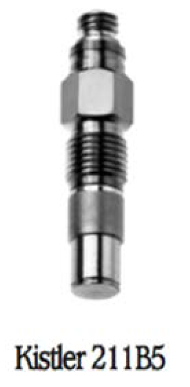
Figure 4.
National Instrument Board and Data Acquisition Equipment.

Figure 5.
Cluster and Location of Channels.

Figure 6.
High-Speed Camera.
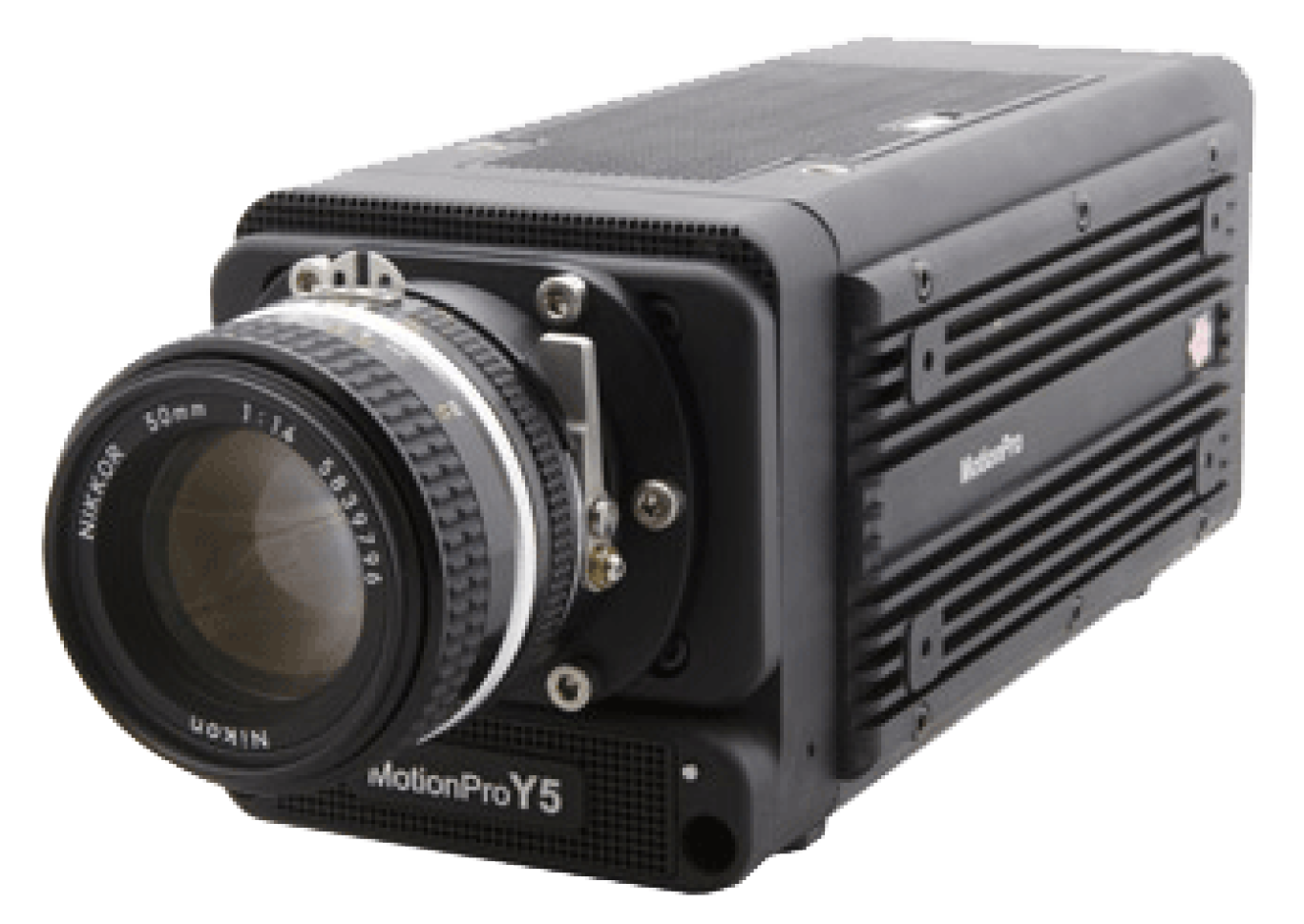
Figure 7.
Scheme of Peak Pressure Detection.

Figure 8.
Snapshots of Flow: SWAY (Dry).

Figure 9.
Snapshots of Flow: SWAY (Wet).
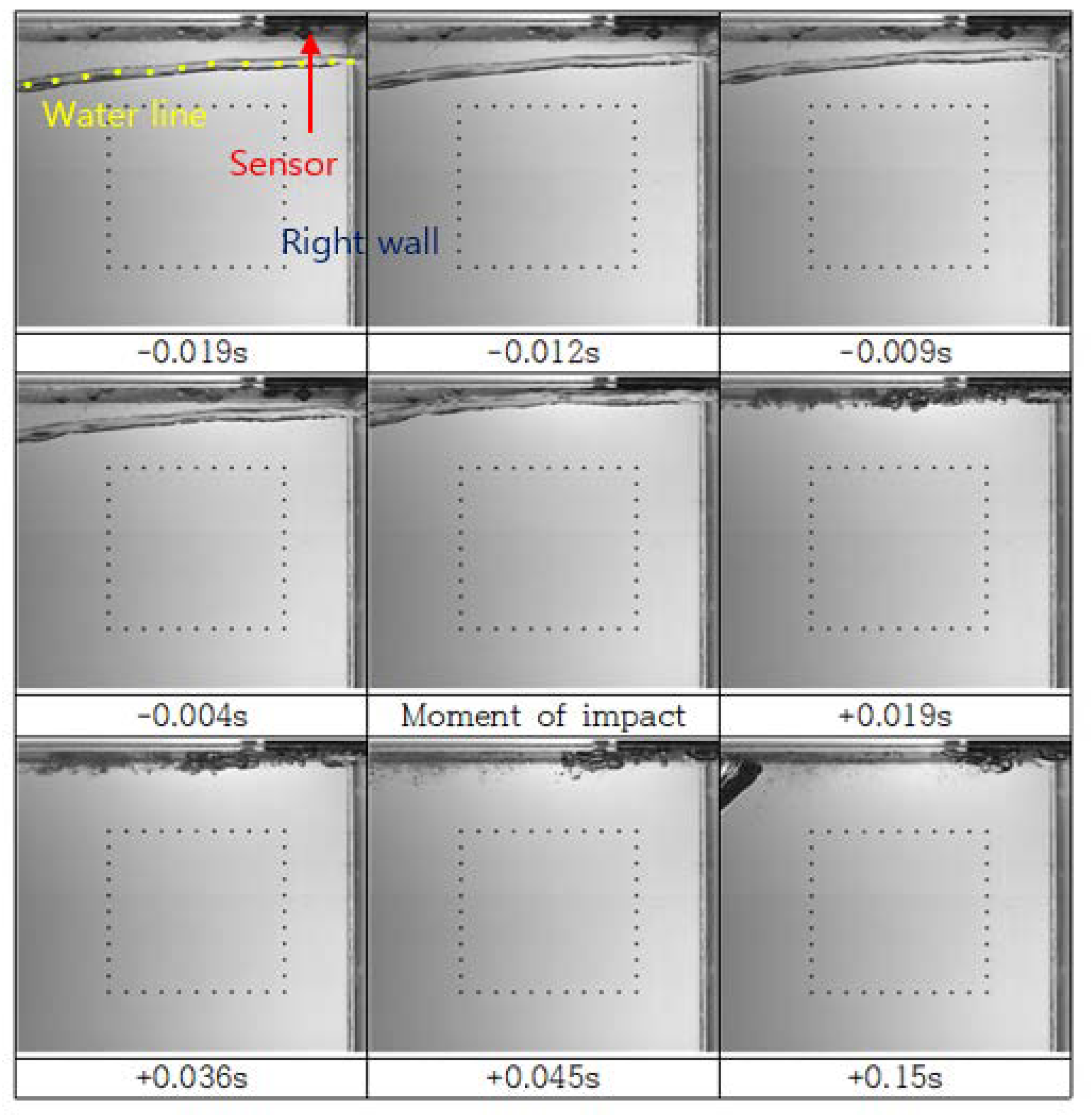
Figure 10.
Snapshots of Flow: ROLL (Dry).

Figure 11.
Snapshots of Flow: ROLL (Wet).

Figure 12.
Snapshots at First Impact: SWAY (Dry).

Figure 13.
Snapshots at First Impact: SWAY (Wet).

Figure 14.
Snapshots at First Impact: ROLL (Dry).

Figure 15.
Snapshots at First Impact: ROLL (Wet).

Figure 16.
Time Histories of the Pressure Measured at Four Different Channels for SWAY (Wet): (a) Channel 46, (b) Channel 51, (c) Channel 58 and (d) Channel 63.
Figure 16.
Time Histories of the Pressure Measured at Four Different Channels for SWAY (Wet): (a) Channel 46, (b) Channel 51, (c) Channel 58 and (d) Channel 63.
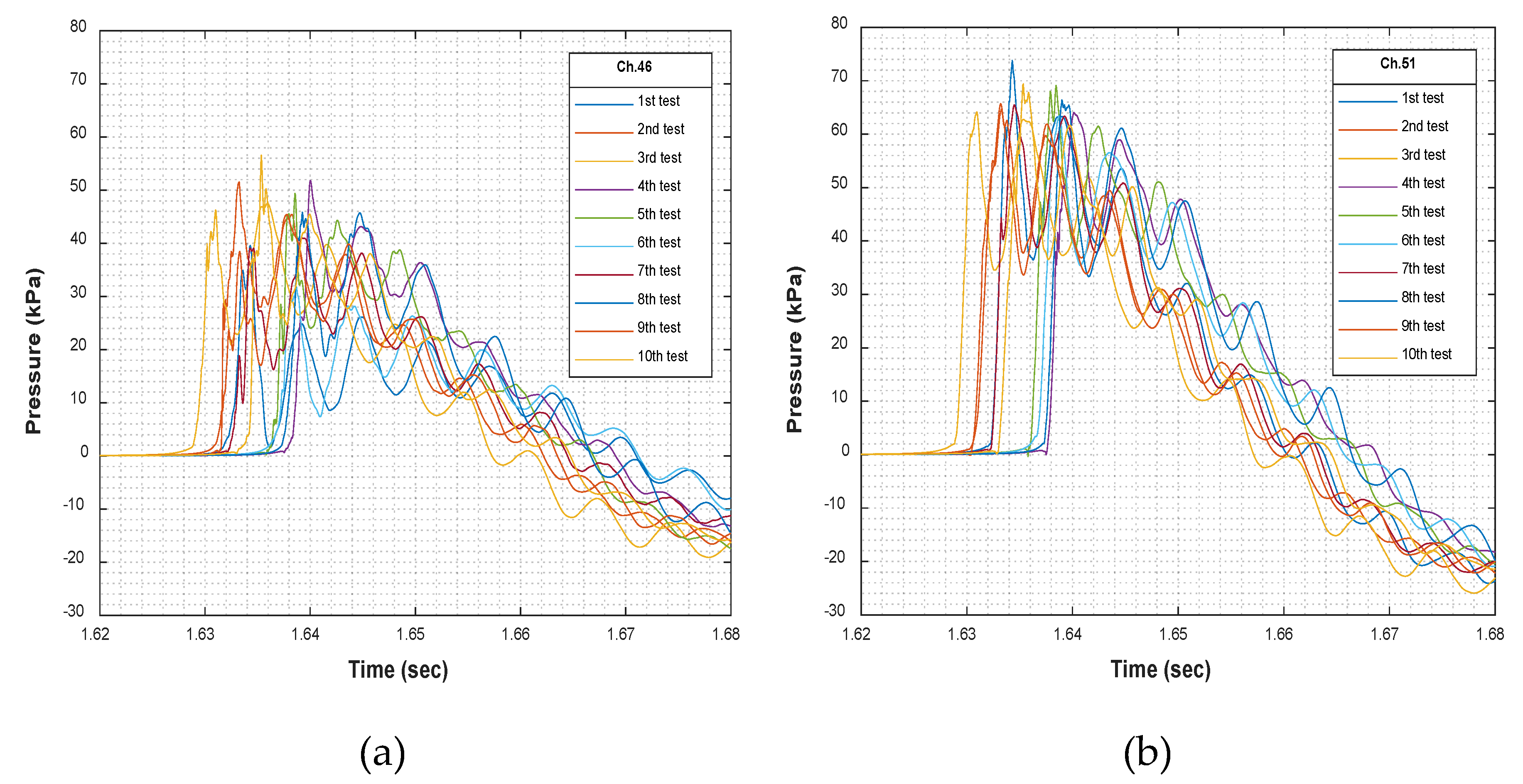

Figure 17.
Time Histories of the Pressure Measured at Four Different Channels for ROLL (Wet): (a) Channel 46, (b) Channel 51, (c) Channel 58 and (d) Channel 63.
Figure 17.
Time Histories of the Pressure Measured at Four Different Channels for ROLL (Wet): (a) Channel 46, (b) Channel 51, (c) Channel 58 and (d) Channel 63.


Figure 18.
FFT of Channel 46 (Wet Condition, SWAY).
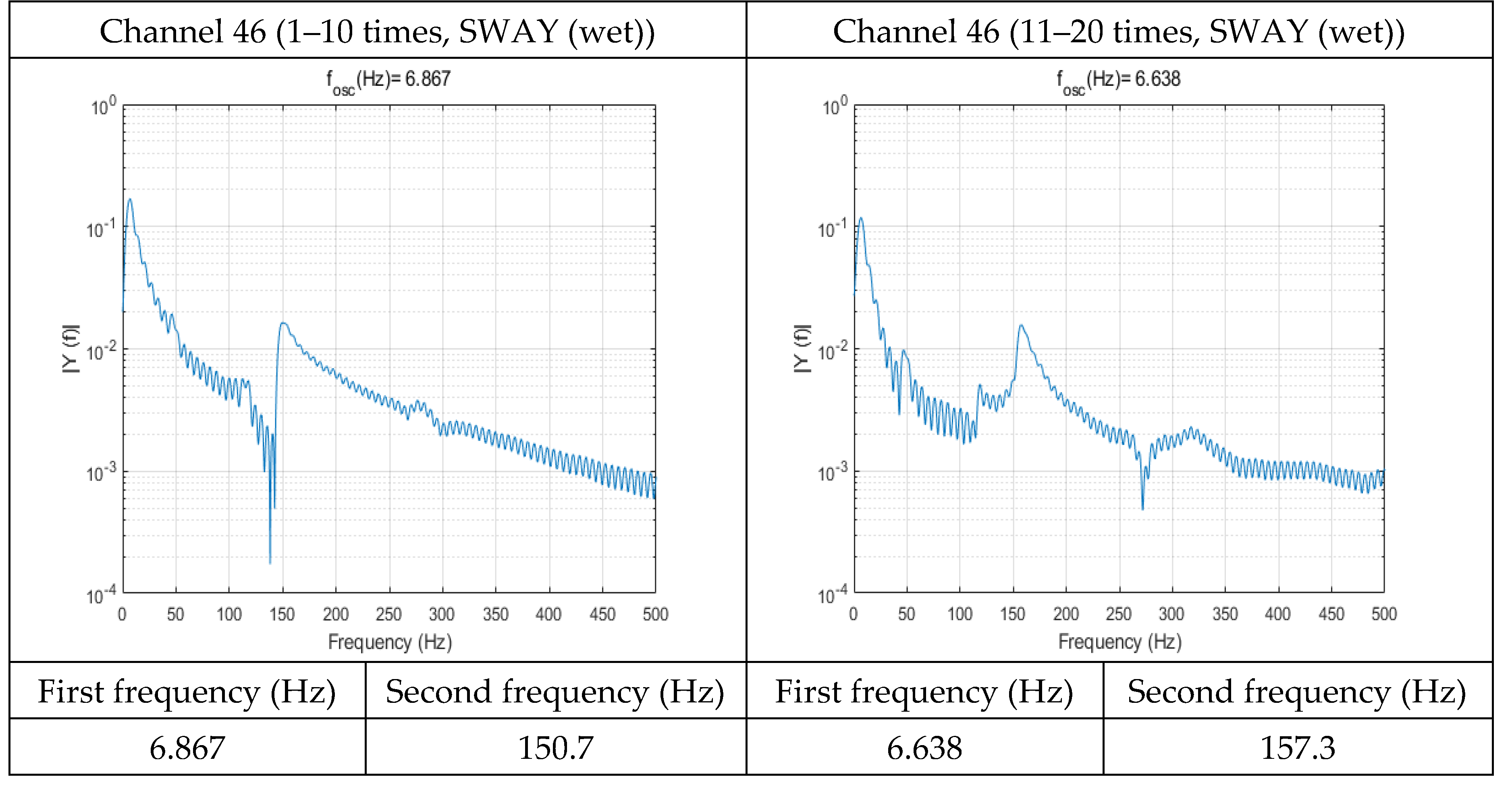
Figure 19.
FFT of Channel 51 (Wet Condition, SWAY)

Figure 20.
FFT of Channel 58 (Wet Condition, SWAY).

Figure 21.
FFT of Channel 63 (Wet Condition, SWAY)

Figure 22.
Peak Pressure of Dry Condition & Wet Condition of SWAY (T1).

Figure 23.
Peak Pressure of Dry Condition & Wet Condition of ROLL (T2)

Figure 24.
Droplet Location of SWAY (the 2nd experiment).
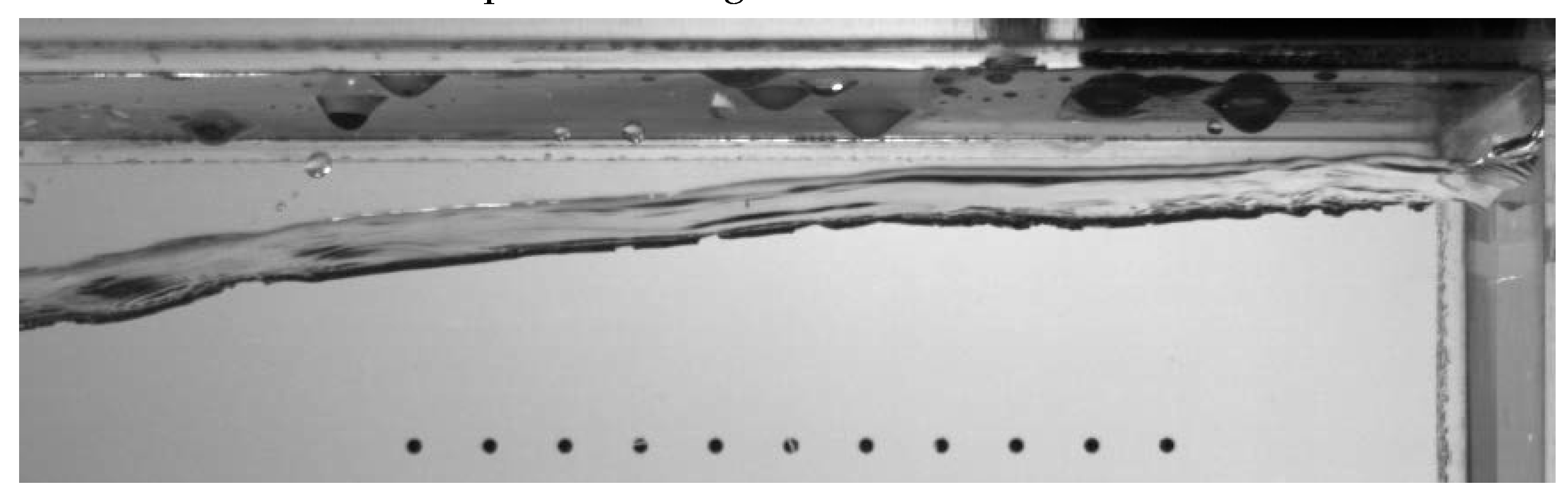
Figure 25.
Droplet Location of ROLL (the 10th experiment).
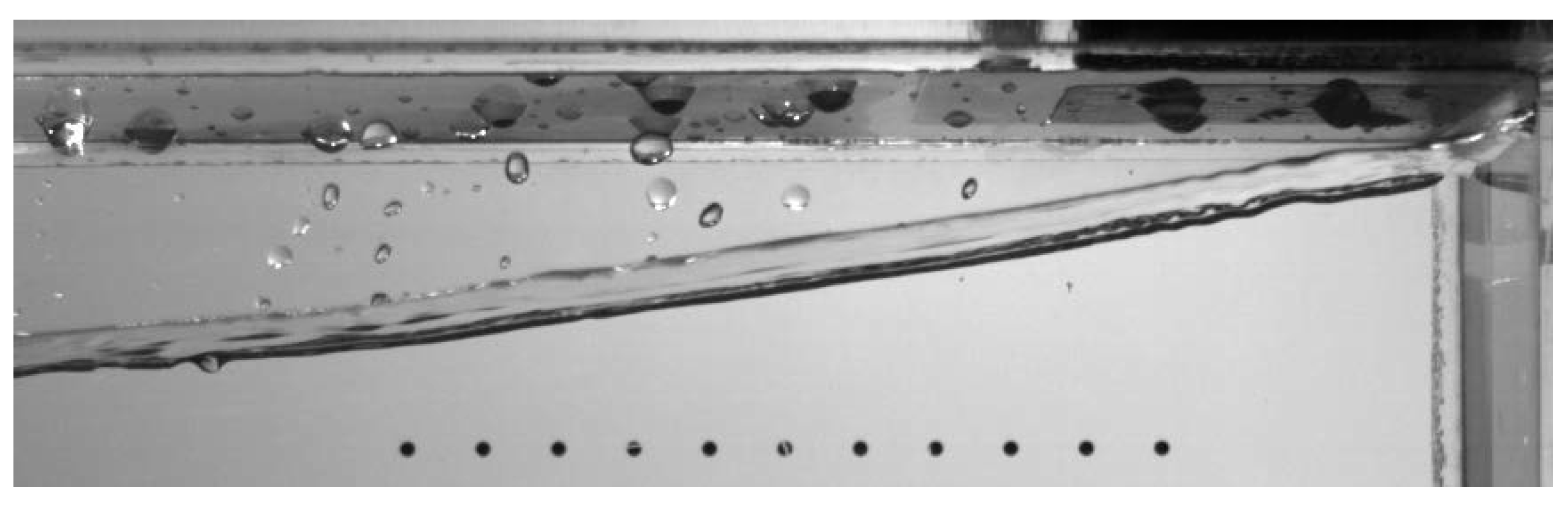
Figure 26.
Peak Pressure of Dry and Wet conditions and the 2nd Experiment in Wet Condition of SWAY (T1); Red circle - the location of the droplets, Orange circle - the vicinity of the droplets.
Figure 26.
Peak Pressure of Dry and Wet conditions and the 2nd Experiment in Wet Condition of SWAY (T1); Red circle - the location of the droplets, Orange circle - the vicinity of the droplets.
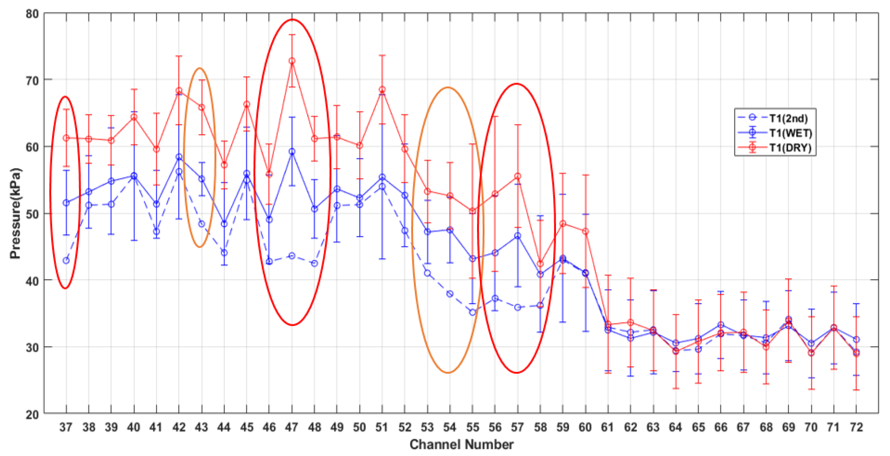
Figure 27.
Peak Pressure of Dry and Wet conditions and the 10th Experiment in Wet Condition of ROLL (T2); Red circle - the location of the droplets.
Figure 27.
Peak Pressure of Dry and Wet conditions and the 10th Experiment in Wet Condition of ROLL (T2); Red circle - the location of the droplets.

Figure 28.
3D Plot for Discrepancy in Peak Pressure (the 2nd Case Pressure - Wet Average, SWAY).
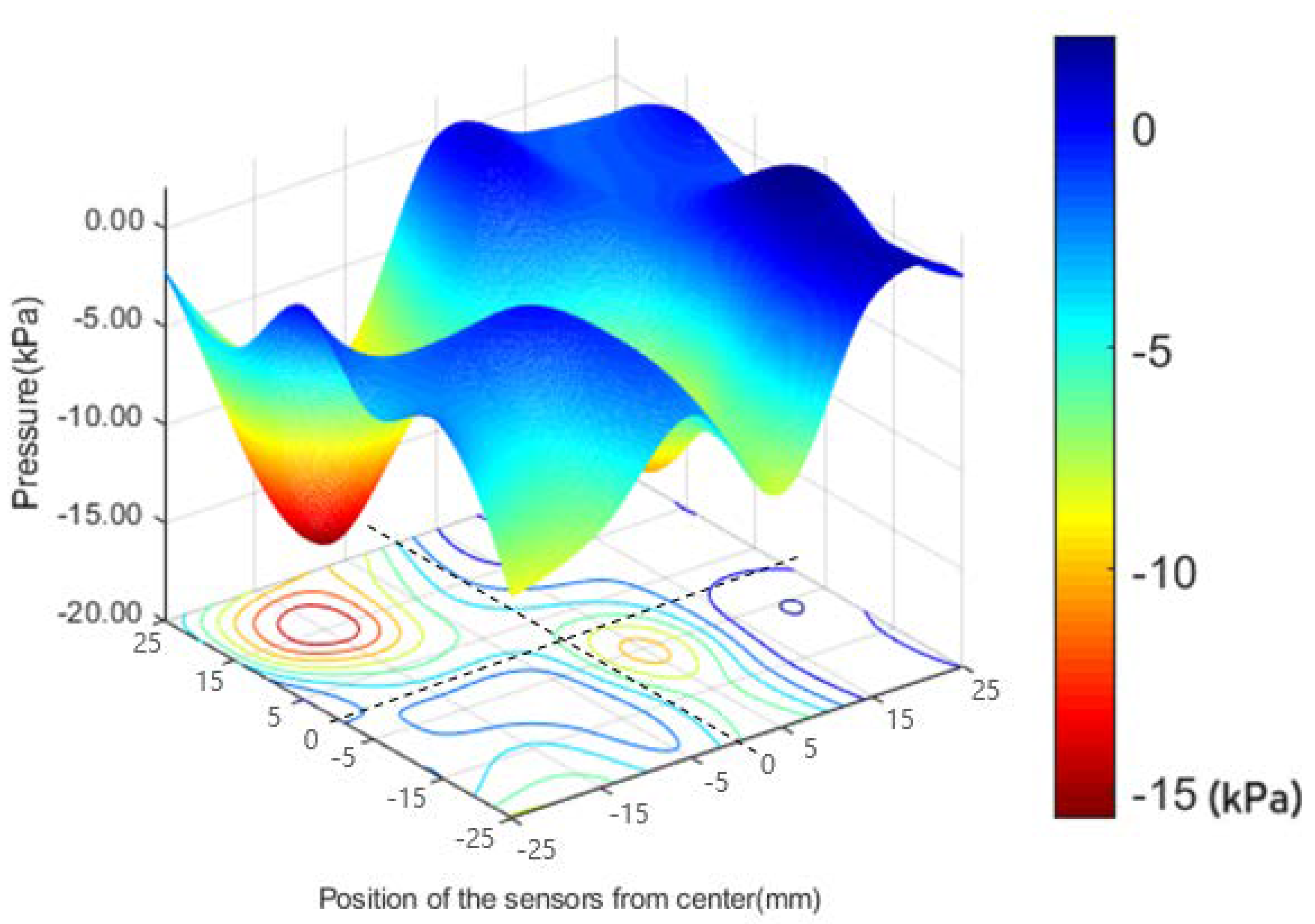
Figure 29.
3D Plot for Discrepancy in Peak Pressure (the 10th Case Pressure -Wet Average, ROLL).

Figure 30.
Contour for Discrepancy in Peak Pressure (the 2nd Case Pressure -Wet Average, SWAY).

Figure 31.
Contour for Discrepancy in Peak Pressure (the 10th Case Pressure -Wet Average, ROLL).

Table 1.
Specifications of Actuator.
| Items | Specification |
|---|---|
| Servo Motor | P60B2215KBXS (SANYODENKI) |
| Servo Driver | PZA300 |
| Rating Power | 15 kW |
| Rating rpm | 1500 rpm |
| Maximum rpm | 2000 rpm |
| Rating Torque | 95.5 Nm |
| Maximum Torque | 240 Nm |
| Ball Screw Lead | 40 mm |
| Maximum Stroke | 1000 mm |
Table 2.
Range of Displacement and Velocity.
| Motion | Displacement | Velocity |
|---|---|---|
| Surge | −1060 mm~1030 mm | 200 cm/s (0.4 Hz) |
| Sway | −970 mm~970 mm | 190cm/s (0.4 Hz) |
| Heave | −540 mm~540 mm | 100cm/s (0.4 Hz) |
| Roll | −34.5°~34.5° | 83 deg/s (0.4 Hz) |
| Pitch | −36.5°~34.9° | 83 deg/s (0.4 Hz) |
| Surge | −1060 mm~1030 mm | 200 cm/s (0.4 Hz) |
Table 3.
Specifications of Pressure Sensor.
| Items | Unit | Kistler 211B5 |
|---|---|---|
| Diameter | mm | 5.5 |
| Range | bar | 0~6.895 |
| Overload | bar | 34.474 |
| Sensitivity | - | 804.2 mV/bar ( |
| Natural Frequency | kHz | 300 |
| Linearity | %FSO | ≤±10 |
| Acceleration Sensitivity | bar/g | 0.0001379 ( |
| Operating Temperature Range | °C | −51~121 |
Table 4.
Specifications of Board and DAQ.
| Items | Specification |
|---|---|
| Analog inputs | 8 Channel |
| Resolution | 24 bits |
| Maximum Sampling Rate | 102.4 kS/s |
| Input Range | ±10V |
| AC Cutoff Frequency | 0.5 Hz |
Table 5.
Specification of the camera.
| Items | Specification |
|---|---|
| Image resolution | 1280 × 1024 at 1000 fps |
| Internal memory | 4 GB |
| Recording rates | Selectable Up to 64,000 fps |
Table 6.
Test conditions.
| Test Condition | Filling Level (%H) | Filling Level (mm) | Excitation Motion | Excitation Periods (s) | Excitation Amplitude (mm or ) | Test Duration |
|---|---|---|---|---|---|---|
| SWAY(T1) | 85 | 570 | Sway | 1.1 | 32 mm | 1 impact |
| ROLL(T2) | 85 | 570 | Roll | 1.207 | 4.5 | 1 impact |
Table 7.
Test temperatures.
| Set | SWAY (Wet) | SWAY (Dry) | ROLL (Wet) | ROLL (Dry) | ||||
|---|---|---|---|---|---|---|---|---|
| Air (°C) | Water (°C) | Air (°C) | Water (°C) | Air (°C) | Water (°C) | Air (°C) | Water (°C) | |
| 1 | 13.4 | 11.6 | 13.5 | 11.3 | 10.2 | 12.8 | 11.1 | 11.2 |
| 2 | 13.4 | 11.6 | 13.5 | 11.6 | 10.0 | 12.8 | 11.2 | 11.2 |
Table 8.
Peak Pressure of Dry condition, Wet condition, Droplet case.
| Test Condition | Channel Number | |||||
|---|---|---|---|---|---|---|
| SWAY | 37 | 61.25 | 51.54 | 42.91 | −29.94 | −16.74 |
| 47 | 72.79 | 59.22 | 43.62 | −40.07 | −26.34 | |
| 57 | 55.53 | 46.62 | 35.90 | −35.35 | −22.99 | |
| ROLL | 47 | 58.20 | 44.91 | 36.65 | −37.03 | −18.39 |
| 56 | 48.84 | 37.52 | 32.21 | −34.05 | −14.15 |
© 2019 by the authors. Licensee MDPI, Basel, Switzerland. This article is an open access article distributed under the terms and conditions of the Creative Commons Attribution (CC BY) license (http://creativecommons.org/licenses/by/4.0/).
Share and Cite
MDPI and ACS Style
Kim, D.H.; Kim, E.S.; Shin, S.-c.; Kwon, S.H. Sources of the Measurement Error of the Impact Pressure in Sloshing Experiments. J. Mar. Sci. Eng. 2019, 7, 207. https://doi.org/10.3390/jmse7070207
AMA Style
Kim DH, Kim ES, Shin S-c, Kwon SH. Sources of the Measurement Error of the Impact Pressure in Sloshing Experiments. Journal of Marine Science and Engineering. 2019; 7(7):207. https://doi.org/10.3390/jmse7070207
Chicago/Turabian StyleKim, Dong Hwi, Eun Soo Kim, Sung-chul Shin, and Sun Hong Kwon. 2019. "Sources of the Measurement Error of the Impact Pressure in Sloshing Experiments" Journal of Marine Science and Engineering 7, no. 7: 207. https://doi.org/10.3390/jmse7070207
Note that from the first issue of 2016, this journal uses article numbers instead of page numbers. See further details here.