Article

Model Behavior and Sensitivity in an Application of the Cohesive Bed Component of the Community Sediment Transport Modeling System for the York River Estuary, VA, USA

by
Kelsey A. Fall
1,*,
Courtney K. Harris
1,†,
Carl T. Friedrichs
1,†,
J. Paul Rinehimer
2,† and
Christopher R. Sherwood
3,†
1
Virginia Institute of Marine Science, College of William & Mary, Gloucester Point, VA 23062, USA
2
Center for Coastal Margin Observation & Prediction, Oregon Health and Sciences University, Portland, OR 97239, USA
3
US Geological Survey, Coastal and Marine Geology Program, Woods Hole, MA 02543, USA
*
Author to whom correspondence should be addressed.
These authors contributed equally to this work.
J. Mar. Sci. Eng. 2014, 2(2), 413-436; https://doi.org/10.3390/jmse2020413
Submission received: 18 December 2013 / Revised: 3 April 2014 / Accepted: 4 April 2014 / Published: 14 May 2014

Abstract

:
The Community Sediment Transport Modeling System (CSTMS) cohesive bed sub-model that accounts for erosion, deposition, consolidation, and swelling was implemented in a three-dimensional domain to represent the York River estuary, Virginia. The objectives of this paper are to (1) describe the application of the three-dimensional hydrodynamic York Cohesive Bed Model, (2) compare calculations to observations, and (3) investigate sensitivities of the cohesive bed sub-model to user-defined parameters. Model results for summer 2007 showed good agreement with tidal-phase averaged estimates of sediment concentration, bed stress, and current velocity derived from Acoustic Doppler Velocimeter (ADV) field measurements. An important step in implementing the cohesive bed model was specification of both the initial and equilibrium critical shear stress profiles, in addition to choosing other parameters like the consolidation and swelling timescales. This model promises to be a useful tool for investigating the fundamental controls on bed erodibility and settling velocity in the York River, a classical muddy estuary, provided that appropriate data exists to inform the choice of model parameters.

1. Introduction

Fine sediment transport in coastal and estuarine environments has significant physical, biological, and chemical ramifications. Mobilized sediments reduce water clarity, transport toxic materials, pathogens and nutrients, and fill navigational channels [1,2]. Bed erodibility and settling velocity are key parameters influencing fine sediment dynamics in coastal and estuarine environments. Bed erodibility controls the amount of sediment suspended while settling velocity influences how far it is transported [3,4,5,6,7]. Erodibility and settling velocity vary widely over time and space in estuaries, and these variations are closely related to sediment flux convergences and divergences at Estuarine Turbidity Maxima (ETMs) [8,9,10,11,12].
ETMs are regions of locally high suspended-sediment concentrations that often occur immediately landward of the salt limit, where convergence in near-bottom flow traps suspended sediment in the bottom layer [13,14,15]. Suspended sediment trapped in the bottom layer near the head of salt cannot be entrained into the upper layer due to damping of turbulent mixing by stratification [16]. Tidal asymmetries in vertical velocity and suspended-sediment profiles can also produce ETMs [9,17,18]. Although these processes tend to be most important near the head of salt, they can create ETMs in other areas where the channel geometry alters the salinity field, often called Secondary Turbidity Maxima or STMS [19,20,21,22]. Hydrodynamic forces and sediment and bed properties influence both ETMs and STMs, and because these factors vary with time and in all three spatial dimensions, they are difficult to study using field measurements alone. A three-dimensional model is helpful for evaluating and understanding these complex processes that influence sediment dynamics in muddy estuaries.
Erosion of sediment from the bed provides an important control on estuarine turbidity. Here we define erodibility (ε) as the asymptotic relationship between a steady, externally imposed bed stress (τb), and total eroded mass from the seabed when τb exceeds the critical stress (τc) of the sediment surface. The critical shear stress, τc, represents the stress at which motion or suspension of sediment first occurs [23]. Erosion rates have been estimated using many different formulas [24,25,26,27], but the simple linear Ariathurai-Partheniades erosion formulation has been assumed in many cases:
E = M(τbτc)
Here, the erosion rate, E (kg m−2 s−1), varies linearly with the excess shear stress (τbτc) (Pa) according to the erosion rate parameter, M (kg m−2 s−1 Pa−1 m−2) [11,12,28,29,30,31,32,33]. Though developed for cohesive sediment, Equation (1) can also be applied to non-cohesive beds. For purely non-cohesive beds, τc mostly depends on the grain size and density of individual particles, and typically increases with diameter [23]. For cohesive sediment, τc represents a bulk characteristic of the seabed, and may depend on grain size, porosity, organic content, and depositional history, and often increases with depth in the seabed and with time since deposition [24].
Many three-dimensional numerical models assume a constant τc, even for cohesive sediment [7,34,35,36], which can produce satisfactory results when applied for short time scales, but neglects feedbacks between erodibility, erosion, and deposition that develop in response to events such as flood deposition, spring freshets, storm erosion, or biogenic seasonal variations [37,38,39,40]. A model of the York River estuary in Virginia that defined a constant value of τc [35,41] was able to represent the STM but underestimated suspended-sediment concentrations, despite using 0.05 mm/s for settling velocity, significantly smaller than the values inferred from recent observations [8,10,42]. More recently, a York River model was implemented to estimate suspended-sediment concentrations associated with Hurricane Isabel [7]. This used Sanford’s (2008) consolidation model [43] that allows τc to vary in response to consolidation. The parameters in their bed consolidation model were based, when possible, on data from the York River, or otherwise from literature values, however the article did not discuss the sensitivity of calculations to these parameters.
In this study we applied a three-dimensional hydrodynamic and sediment-transport model to represent processes in the York River estuary, VA, USA, using the Community Sediment Transport Modeling System (CSTMS) with a cohesive bed sub-model [33]. The critical shear stress profile of the cohesive bed was estimated following the consolidation and swelling model presented in [43]. The objectives of this paper are to (1) describe the application of the three-dimensional hydrodynamic York cohesive bed model, (2) compare calculations to observations, and (3) investigate sensitivities of the cohesive bed sub-model to user-defined parameters.

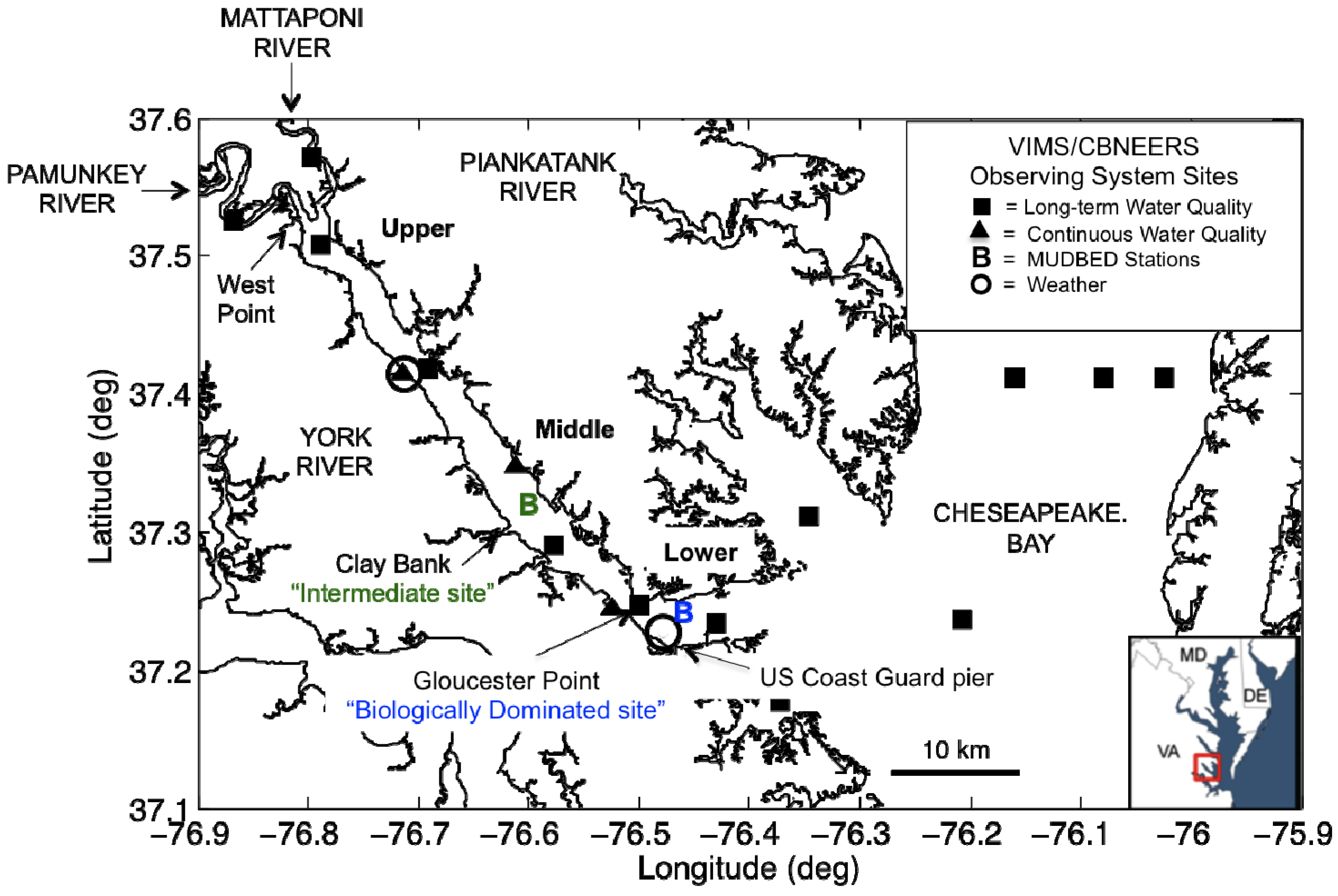
2. Study Site: York River Estuary, VA, USA

The York River (Figure 1), a partially mixed microtidal estuary, spans 50 km from West Point to Gloucester Point [44]. Tidal currents approach 1 m/s at the water surface and dominate sediment resuspension [45]. The estuary contains a main channel (~5–20 m deep) and a secondary channel (~5 m deep), both dominated by mud, and bordered by well-developed sandy shoals (~2 m deep) [44,46]. The primary ETM occurs upstream near West Point. A secondary turbidity maximum (STM) occurs about 40 km landward of the river mouth in a mid-estuary transition region near the Intermediate site between the well-mixed zone upriver and more stratified zone seaward [20]. Physical processes dominate in the upper and middle York, where the benthic diversity, productivity and biomass are suppressed by the more intense tidal currents, greater range of salinities, and the ephemeral presence of the STM [44]. In the lower York, near Gloucester Point, the estuary turns toward the northwest, widens from about 3 km to 6 km, and the main channel depth increases to 20 m. As a result, the seabed is only disturbed during storms, and suspended-sediment concentrations are lower (10 s of mg/L), creating a more favorable environment for benthic organisms [45].
Figure 1. Map of York River estuary, southeastern VA, USA. The location of the Multidisciplinary Benthic Exchange Dynamics (MUDBED) Intermediate site is in green and MUDBED Biologically Dominated site is in blue.
Jmse 02 00413 g001
The York River estuary has been studied as a part of the Multidisciplinary Benthic Exchange Dynamics (MUDBED) project [4], particularly near Clay Bank at the MUDBED Intermediate site, and near Gloucester Point at the MUDBED Biologically Dominated site (Figure 1). The seabed at both sites is dominated by mud and resilient biologically repackaged fecal pellets, with very little sand [47,48]. Individual mud particles and flocculated muds form the major fraction of suspended material in the York. Repackaged fecal pellets are suspended during periods of high bed stresses [42].
While data from the Biologically Dominated site revealed little variability in either settling velocity or erodibility, at the Intermediate Site long-term observations from the MUDBED benthic Acoustic Doppler Velocimeter (ADV) tripod [4,10] and Gust microcosm experiments [11] showed temporal variability in sediment settling velocity and bed erodibility. During the late winter and spring (February–May), erodibility at the Intermediate site generally exceeded that during the summer and fall, with the most erodible beds occurring in April and May [11]. Settling velocities based on ADV data, and bed erodibilities estimated by the Gust microcosm and ADV data were inversely correlated at the Intermediate site, with lower settling velocities observed during periods of increased erodibility, while settling velocities increased during periods of reduced erodibility [10].
Observations indicated that the temporal variability in bed erodibility and settling velocity at the Intermediate site can be attributed to the presence or absence of the STM [4,11,49]. At times of high river flow, stratification of the water column increased, and slowly settling, easily erodible flocculated muds became trapped as the STM formed. The STM migrates along the middle reach of the estuary over pools of easily erodible, muddy sediment [11,20], similar to “mud reaches” observed in other estuaries including the Hudson [37] and the Weser [50]. During periods of elevated river flow, high suspended-sediment concentrations associated with the STM, in combination with increased salinity stratification, dampened near-bed turbulence and prevented the suspension of faster-settling biologically repackaged material [49]. When river discharge dropped, stratification decreased, allowing fine sediment to disperse through the water column, reducing sediment-induced stratification. This permitted higher bed stresses that could suspend the less erodible, faster settling biologically repackaged pellets in addition to slowly settling muddy flocs, so that lower bulk erodibility and higher bulk settling velocities were observed at the site.
The York River estuary is a cohesive and highly dynamic sedimentary environment subject to the presence of a seasonal STM [20]. Erosion and deposition occur alternately, resulting in temporal and spatial variability in seabed τc profiles [11,47]. Therefore, a cohesive bed model that accounted for time varying τc profiles would best represent the York and could be based on observed seabed profiles.

3. Methods

A three-dimensional representation of the York River estuary was developed using the Regional Ocean Modeling System (ROMS) v3.1 [51,52]. ROMS solves the hydrostatic Reynolds-averaged Navier-Stokes equations on a curvilinear orthogonal grid with vertical stretched terrain-following coordinates. ROMS provides a choice of boundary conditions, advection schemes, turbulence parameterizations, and sub-models for sediment transport [53]. Our implementation modified a previously described model [54] by adding wind forcing and updating parameters. We used ROMS options for the Mellor and Yamada level 2.5 turbulence closure model [55], a third-order upstream advection method for momentum, and the MPDATA advection method for tracers such as sediment [56]. Bottom drag was parameterized with a logarithmic current velocity profile [57] with a bed roughness of 0.005 cm based on observed bed stresses (discussed below). The ROMS sediment model of [53] was included but modified to account for consolidation and swelling processes following [43] and [33] as described below. The model run simulated two months after first completing month spin-up, and the model performance was evaluated using values obtained from ADV observations. Additionally, we investigated sensitivities of the cohesive bed model to two user-defined parameters.

3.1. Cohesive Bed Model

The CSTMS cohesive sediment bed model is based on [43] and represents consolidation and swelling processes, and an increase of τc with depth in the sediment, which is typically observed in muddy seabeds. A brief summary of the model implementation in ROMS follows, see [33,58] for more detail. The model represents the seabed at each horizontal grid point as a stack of several bed layers, and stores a value of the critical shear stress for erosion, τc (m), at the top of each bed layer, with m (kg m−2) being the sediment mass overlying that layer. Under erosional conditions, surficial sediment is entrained into suspension, and the τc at the bed surface increases as sediment having a higher τc becomes exposed. During times of deposition, the model assumes a low critical stress, τc = 0.01 Pa, for newly deposited material, creating an easily erodible layer at the bed surface.
Relaxation equations account for the temporal effects of consolidation and swelling on τc [43]. The bed sediment is assumed to have an equilibrium critical stress profile τceq (m). At the end of every model time-step, the instantaneous critical stress profile, τc (m), is nudged toward τceq (m) to simulate consolidation and swelling according to:
Jmse 02 00413 i001
where Tc and Ts are timescales for consolidation and swelling processes, respectively. Reasonable ranges for Ts are suggested to be on the order of 100 days, while the Tc is expected to be much shorter at around one day [42]. Following [33], profiles for τceq were based on power law fits to erodibility experiments performed by [48] on cores collected in September, 2007, and April, 2007 (Figure 2).
Figure 2. Profiles of τceq obtained by power law fit to observations (as in [33]). Power law fit to observed (solid lines) critical stress profiles for April and September, 2007. Triangles and asterisks show observed data from [48].
Jmse 02 00413 g002
The model calculates erosion when bed shear stress (τb) exceeds τc at the sediment surface (Equation (1)). In its original form, the model allowed M to vary with depth as a function of solids volume fraction φs [43]. As implemented here, however, both solids fraction and the erosion rate parameter were held constant with φs = 0.1 and M = 1 × 10⁻³ kg/m2 s Pa. Previous analysis concluded that erosion in the York River was primarily depth-limited and hence depended more on the critical stress profile than on the erosion rate parameter [33]. The York River model calculated bed stress assuming a logarithmic current profile in the bottom boundary layer. Stresses were computed by ROMS subroutine uv_logdrag from the velocity in the bottom cell and a user-defined hydraulic roughness parameter (Z0) [53,54]. Based on observations Z0 was defined as a constant 0.005 cmab.

3.2. Implementation of Three-Dimensional York River Hydrodynamic Cohesive Bed Model

This describes the three-dimensional York River hydrodynamic cohesive bed model, originally developed by [55], and the more recent modifications used in this study. The “Standard Model” refers to the version that best matched observations from the Intermediate site on the York River. Later sections evaluate the sensitivity of calculations to changes in model parameters by comparing results from the Standard Model to those from other implementations.
The horizontal model grid of [41] adopted for this study had an average grid resolution of 170 m in the along-channel direction and 110 m in the cross-channel direction (Figure 3). The major tributaries of the York, the Mattaponi, and Pamunkey Rivers, were represented in the model with only one cell in the cross-channel direction due to their narrow width. The model extended about 60 km up-river from West Point, VA, USA to Hanover, VA, USA on the Mattaponi River, and Beulahville, VA, USA on the Pamunkey River. The vertical grid used stretched terrain-following coordinates, with 20 stretched grid layers, and increased resolution at the seafloor and water surface.
Figure 3. The York River estuary cohesive bed ROMS model grid used in in this study had 92 across channel cells and 334 along channel grid cells. Each square in the figure represents twenty-five model grid cells. This paper focuses on model results from the area around the Intermediate site (Clay Bank, VA, USA), which is marked with a black circle.
Jmse 02 00413 g003
Velocity and salinity estimates from the final time step of a spin-up model were used to initialize the hydrodynamic model presented here. For this spin-up, ROMS was run for 60 days including a spring-neap tidal cycle with 0.2 m neap amplitude and 0.4 m spring amplitude. The spin-up model used a steady river input equal to the 60-year median freshwater flows of 42 m3/s and 25 m3/s from the Pamunkey and Mattaponi Rivers, respectively [59].
Calculations included two cohesive sediment classes having settling velocities of 2.4 mm/s and 0.8 mm/s. These values were based on observed settling velocities of the two dominate particle types in suspension, biologically repackaged pellets and flocculated muds [42,49]. The sediment bed was initialized having a total bed thickness of 1 m, with a uniform distribution of sediment types, containing 20% of the coarser sediment class and 80% of the finer sediment class. Bed τc throughout the grid was initialized as the power law fit used by [33] to represent the September profile, τcinit (m) = 1.0 m0.62, while the τceq profile was defined by the power law fit to the more erodbile April (more erodible) profile, τceq (m) = 0.4 m0.55 (Figure 2). Model sensitivity tests, presented in Section 5.2, found that this configuration produced a better match between calculations of suspended sediment concentrations and observed values, compared to other configurations studied. A consolidation timescale of Tc = 1 day and a swelling timescale of Ts = 25 days were used. The model configuration, specifically the model simulation time, must be considered when defining τcinit, τceq, Tc and Ts, as discussed further in Section 6.2. In the runs presented here, the model simulation time of only 120 days included 90 days of spin-up time. With this short simulation time the model instantaneous τc profiles were sensitive to τcinit and Ts, because of the limited time for the bed to adjust towards τceq.
The model was then run to represent May–August, 2007. Results from May to June were treated as spin-up for the sediment field, and our analysis centered on results from July-August, which coincided with ADV deployment. Freshwater discharges were specified using data from USGS gages 1,674,500 near Beulahville, VA, USA for the Mattaponi River and 1,673,000 near Hanover, VA, USA for the Pamunkey River. Suspended-sediment concentrations at these boundaries were set at 5 mg/L. The value chosen approximates typical suspended-sediment concentrations at the boundaries. Material from upriver sources generally remains trapped at the primary ETM at West Point and therefore has little influence on conditions downstream. Wind velocities were assumed to be spatially uniform, and hourly velocities measured at the York Coast Guard Meteorological station near Gloucester Point (see Figure 1, weather station) were used as model input.
The open boundaries at the mouth of the river where the York River meets Chesapeake Bay were specified as follows to account for tides, sediment fluxes, and the salinity gradient. For sea surface elevation, we used data from about 10 km upstream at the US Coast Guard pier (see Figure 3 for location). To improve the agreement between the modeled and observed time series of water elevation at the Coast Guard pier, the data was lagged by 1 h and scaled by a factor of 1.4 before being applied at the open boundary [54]. For the suspended-sediment open boundary condition, a zero-gradient condition was applied.
Salinity in the interior of the model was calculated as a state variable, but near the open boundary the salinity gradient was specified as follows using an empirical relationship that assumed the salinity along the river fit the hyperbolic tangent function [57],
Jmse 02 00413 i002
where S0 was the maximum salinity at the river mouth, X was the along-channel distance, and β was a length scale for the salt intrusion, based on river flow. These were used to estimate the cross-channel averaged salinity, S(x) The along-channel gradient at the open boundary could then be specified from the derivative of Equation (3) with respect to X,
Jmse 02 00413 i003
where s1 and Jmse 02 00413 i004 were the salinity and the salinity gradient at the first interior grid point. The salinity at the boundary s0 was then defined as:
Jmse 02 00413 i005
where Δx was the along channel grid cell width. Data from the Chesapeake Bay Program [60] were used to fit β in Equation (3). Best fit values of β were then regressed against a four-day running mean, four-day lagged river flow (Q4) resulting in β = 290/Q4 + 50. These data fit the hyperbolic tangent function (Equation (3)) with r2 = 0.65. The exercise described above (Equations (3)–(5)) was used to set a flow-dependent open boundary condition for salinity, as has been done for a model of the Hudson River estuary [57].

3.3. Acoustic Doppler Velocimeter (ADV) Observations

Sontek ADV Ocean Probes have been maintained nearly continually at the MUDBED Intermediate site since 2006 (see Figure 1). The ADVs were attached to bottom-mounted tripods and measured three-dimensional water velocity (u,v,w) and acoustic backscatter at roughly 35 cm above the bed, see [10] for details of the instrumentation. This project used observations collected by a 5MHz ADV deployed from June to August 2007 to estimate burst-averaged bottom stress (τb, via Reynolds averaging of turbulent velocity), suspended-sediment concentration (C, via acoustic backscatter calibrated by pump samples), and bulk sediment settling velocity (WsBULK, via an assumed Rouse balance between upward Reynolds flux and gravitational settling) [8,10,61].

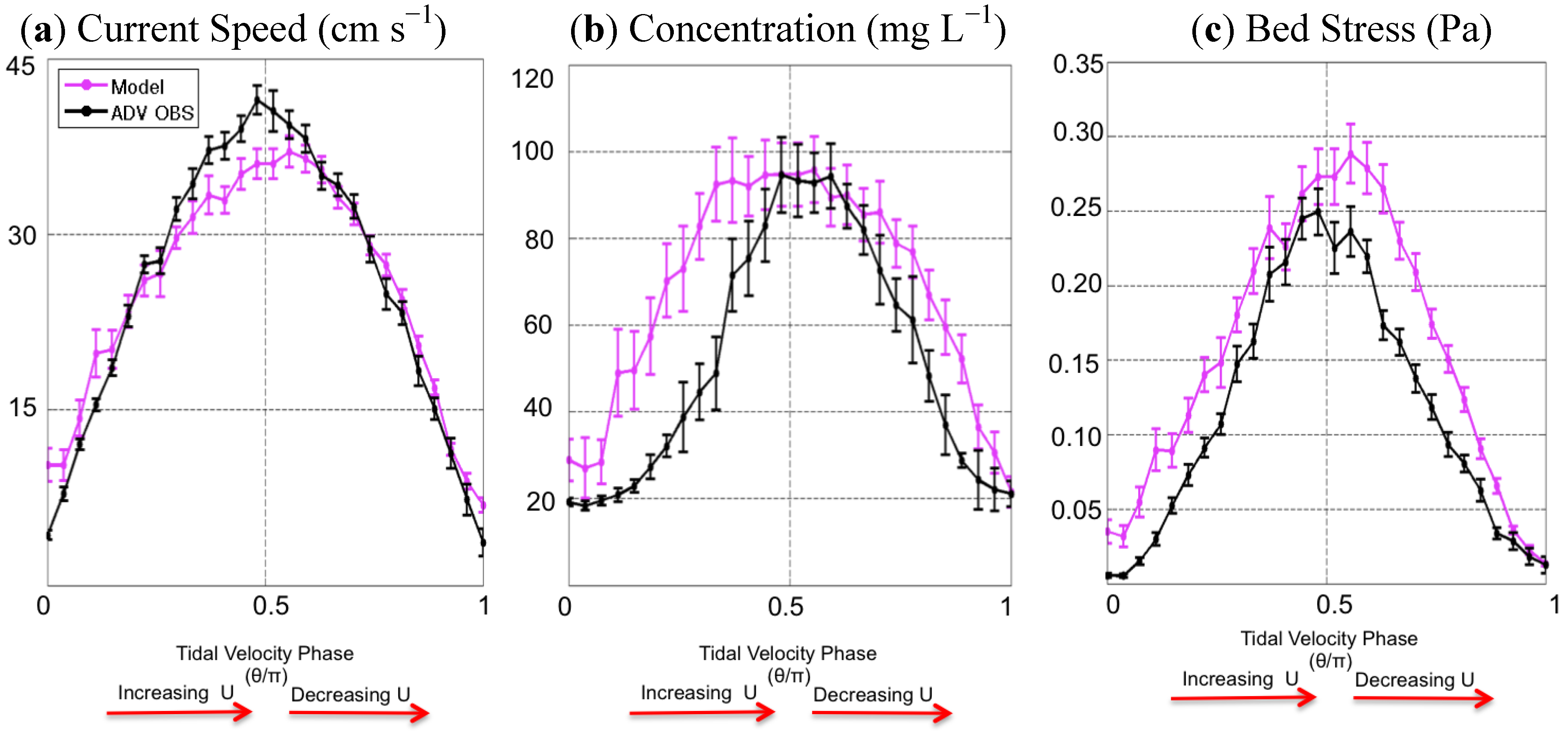
3.4. Standard Model Evaluation

The Standard Model, run from July–August 2007, encompassed a time period for which ADV data and bed samples from the Intermediate site were available. This study especially focused on model behavior over individual tidal phases at the MUDBED Intermediate site. Model estimates from a three-by-three set of adjacent grid cells were averaged to represent the Intermediate site (Figure 3, black dot). These grid cells were chosen because they were within the area where the ADV tripod was deployed, these model cells had water depths similar to that of the observations (~5–6 m), and previous studies collected sediment cores from this location [48].
Data averaged over tidal phases collected by the ADV during this study period has been analyzed to examine the influence of the presence and departure of the STM on sediment dynamics, using the tidal cycles having the top 20% of the observed bed stresses [49]. Typically, bed stresses in the York estuary are low, (tidal max τb < 1 Pa [62]). Our focus on the most energetic tidal cycles did bias our analysis towards spring-tide periods relative to neap-tide periods, but highlighted the study on times when significant sediment would be suspended from the bed. Tidal cycles were defined using the time series of ADV observed current speed (U), such that an individual ebb or individual flood formed a full cycle, with its beginning and end corresponding to times of minimum observed U. Observations over the tidal cycles were then interpolated to a common interval in the tidal phase to produce tidal-phase averaged values of U, τb, C and WsBULK. No distinction was made between floods and ebbs, removing any flood-ebb asymmetry.
Model results from the Standard Model were phase averaged to obtain representative values of hydrodynamic parameters (U, τb, C, and WsBULK). Model estimates of these values were interpolated to the height of the ADV measurements (~35 cmab) prior to the tidal-phase averaging, and model performance was assessed based on the degree to which model calculations of these values represented those derived from ADV observations. The observed estimates of WsBULK were obtained by assuming a Rouse balance, while WsBULK from model results were estimated as the average of the settling velocities of the two size classes (2.4 mm/s and 0.8 mm/s), weighted by their respective suspended-sediment concentrations at the height of the ADV sensor. Though they used different methods, both the model-calculated WsBULK and ADV-based values provided a bulk settling velocity that accounts for all particle sizes present in suspension [63].
Modeled estimates of bed erodibility were calculated by evaluating the depth of the sediment bed that could be resuspended by bed stresses that exceed some threshold, following the definition presented by [11]. For example, the instantaneous profile of critical bed stress (τcinit) estimated for a location in the model typically had a low value at the sediment-water interface and increased with depth in the bed (m). The depth at which the critical stress exceeded the threshold of, e.g., 0.2 Pa, would give a model estimate of the erodibility of the bed at τb = 0.2 Pa. Because the (τcinit) changed in response to erosion, deposition, consolidation, and swelling, the model estimates of erodibility varied in both time and space.

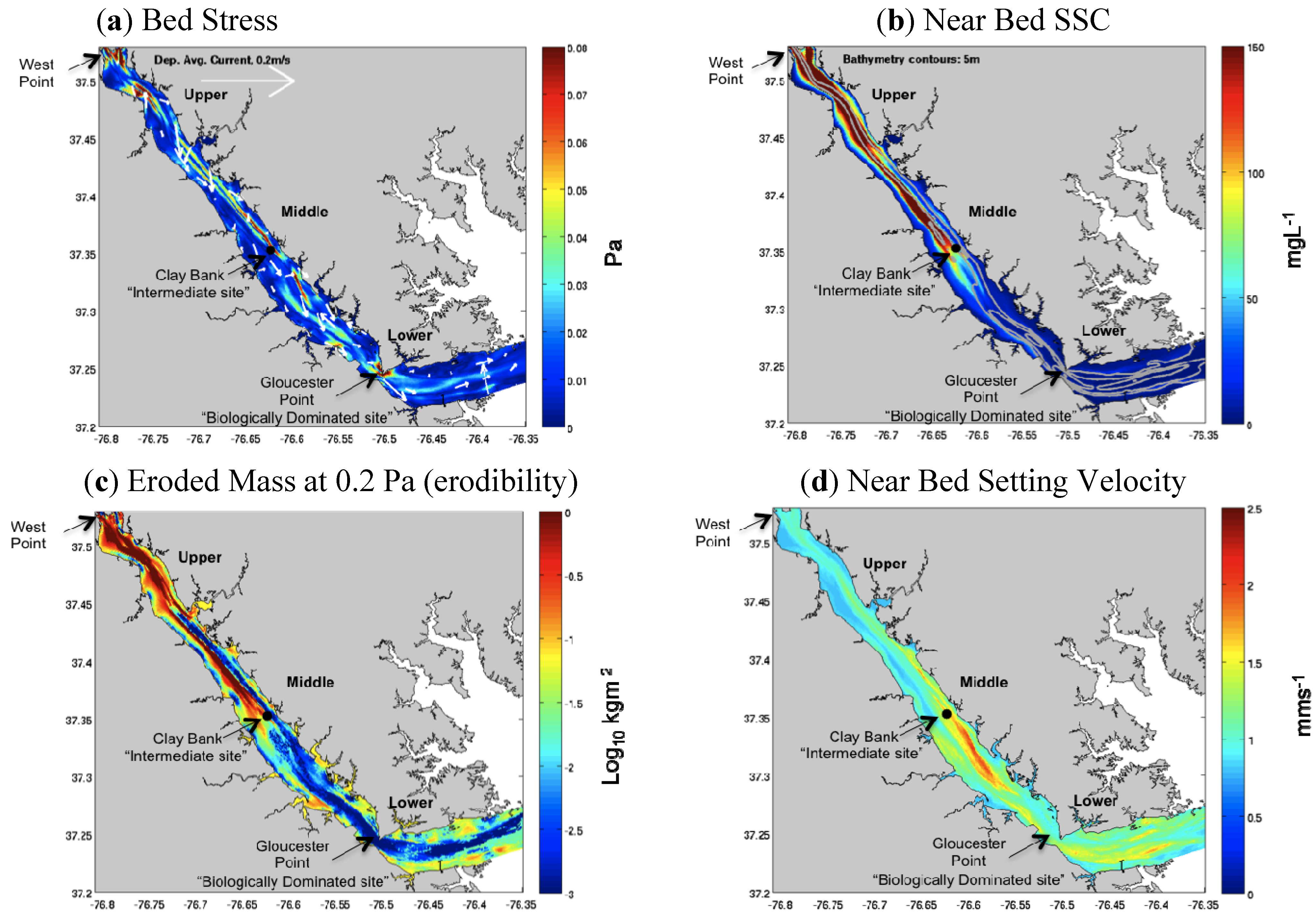
4. Standard Model Results

System behavior is illustrated during times of high (Figure 4) and low (Figure 5) sediment bed erodibility, showing daily-averaged bed stresses, near-bed suspended-sediment concentrations, erodibility at 0.2 Pa, and near-bed settling velocities throughout the York River. These time periods corresponded to a spring tide (Figure 4) and a neap tide (Figure 5). At both times, the upper and middle estuary had increased erodibility and suspended-sediment concentrations, compared to the lower estuary. Both times had similar bed stresses (Figure 4a and Figure 5a), but when erodibility was higher (Figure 4), more material was suspended, having ~0.9 kg m−2 more material in suspension than during the less erodible situation in Figure 5. The increased concentrations were associated with lower near bed settling velocities, particularly in the middle estuary (Figure 4b,d). Ten days later, erodibilty was lower (Figure 5), and decreased suspended-sediment concentrations (~100 mg/L) and higher near-bed settling velocities characterized conditions in the middle estuary (Figure 5b,d). This result was consistent with field observations indicating that during periods of high erodibility, the suspended material was composed of more slowly settling flocculated muds [10,11,48]. The model was also able to capture observed trends in erodibility attributed to the spring/neap tidal cycle. Generally, the sediment bed is more erodible during spring tides and less erodible during neap tides [64].
Figure 4. Daily-averaged model estimates of (a) bed stress, (b) near bed suspended sediment concentration, (c) mass eroded at 0.2 Pa, and (d) near bed settling velocity during a spring tide when high erodibility was found mid-estuary (15 July 2007).
Jmse 02 00413 g004
The results of the tidal-phase average analysis for current speed, concentration, and bed stresses from the model were compared to the ADV estimates from [49]. The model reproduced realistic patterns of all of the parameters over individual tidal cycles. Both model and observed bed stresses and concentration increased with current speed (Figure 6). Peak bed stresses and current speeds in the model had an offset lag compared to the observations (Figure 6a,c). This suggested that the modeled tides may have been slightly out of phase with the observed ones. Overall, the model had more skill at predicting tidal-phase averaged current speeds than the other values considered (Figure 6a). Only at peak flow did model current speeds show a slight bias, underestimating measured speed by less than 5 cm/s (about 12%). The model overestimated suspended-sediment concentrations during the accelerating and decelerating phases of the tide, but matched the concentrations at peak flow (Figure 6b). Bed stresses were overestimated in the model over the entire tidal phase by as much as 0.05 Pa (~18%) (Figure 6c), but this bias was accepted because the modeled currents and sediment concentrations matched reasonably well.
Figure 5. Daily-averaged model estimates of (a) bed stress, (b) near bed suspended sediment concentration, (c) mass eroded at 0.2 Pa and (d) near bed settling velocity during a neap tide when lower erodibility was found mid-estuary (25 July 2007).
Jmse 02 00413 g005
The most reliable approximation of WsBULK from ADV data was obtained during the accelerating portion of the tidal phase, when the assumptions in the Rouse balance were most likely to be appropriate [49]. During the accelerating phase of the tide, the tidal-phase averaged analysis showed that observed WsBULK increased from about 1 mm/s to 1.4 mm/s (Figure 7). More specifically, the tidal-phase averaged analysis showed that observed WsBULK increased from about 1 mm/s to 1.4 mm/s during the accelerating tide (Figure 7). The model represented the observed changes in WsBULK seen in the phase averaged analysis, with modeled WsBULK increasing from about 0.9 mm/s to 1.7 mm/s, though the model estimated slightly higher (~0.3 mm/s) WsBULK at peak bed stresses.
Figure 6. ADV and model estimated (see legend) (a) current speed, (b) concentrations, and (c) bed stresses for the top 20% of tidal cycles with strongest bed stresses. Error bars denote ±1 standard error.
Jmse 02 00413 g006
Figure 7. ADV and model estimated (see legend) bulk settling velocity during periods of increasing tidal velocity for the top 20% of tidal cycles with the highest bed stresses. Error bars denote ±1 standard error.
Jmse 02 00413 g007

5. Cohesive Bed Sub-Model Sensitivity

Additional model runs were analyzed to investigate the sensitivity of the cohesive bed model to the swelling time (Ts), critical shear stress equilibrium profile (τceq), and initial critical shear stress profile (τcinit). The sensitivity to Ts (section 5.1) was evaluated by varying it from 2 to 50 days, bracketing the value of 25 days used in the Standard Model. To test the sensitivity to τceq and τcinit (section 5.2), models were run that defined τceq = τcinit using power-law fits based on the September or the April data (Figure 2). Recall that in the Standard Model, the equilibrium and initial critical shear stress profiles differed as τceq was based on the April power law fit, while τcinit was based on the September profile.

5.1. Sensitivity to Ts

Results from model runs that used different values of Ts (specifically 2, 25, and 50 days) were compared to investigate the sensitivity of the instantaneous τc profiles and resultant suspended-sediment concentrations to swelling timescale. The model configurations were identical to the Standard Model except for the swelling timescales to isolate the influence of Ts. As for the Standard Model, different critical stress profiles were used to initialize the model, and for the equilibrium state toward which the model calculations were nudged (τceq). Bed τc throughout the grid was initialized as the power law fit used by [33] to represent the September sediment bed profile while the τceq profile was defined by the power-law fit found to represent the April (more erodible) profile (Figure 2). Ts = 25 days was used in the Standard Model described above.
Figure 8 shows the values of daily calculated instantaneous τc profiles, along with the user-defined τceq and τcinit for these three models. Recall, the model simulations defined τceqτcrinit. When a short Ts of two days was defined (Figure 8a) the instantaneous τc profiles rapidly became more erodible as the bed adjusted from the less erodible τcinit to the more erodible τceq. When a longer Ts of 50 days was defined (Figure 8c) the instantaneous τc profiles showed minimal adjustment from τcinit to τceq, so that the bed remained more consolidated. In the Standard Model, where Ts was defined as 25 days, the instantaneous τc profiles adjusted somewhat from the less erodible τcinit to τceq.
Figure 8. Daily instantaneous model calculated τc profiles (colored lines) shown with user defined equilibrium (τceq) and initial bed profiles (τcrinit) for model runs with swelling times defined as (a) 2 days, (b) 25 days, and (c) 50 days. Note: τceqτcrinit. Black arrows show the directions that Equation (2) will nudge the instantaneous τc profiles toward τceq.
Jmse 02 00413 g008
Figure 9 compares the resulting tidal-phase average concentrations from these three models and the values derived from ADV observations. The concentrations increased as Ts decreased. Comparison of the three model simulations suggested that using a Ts of 25 days resulted in the most realistic estimates for suspended-sediment concentration, justifying the choice of Ts = 25 days in the Standard Model.
Figure 9. Phase-averaged concentration from ADV observations (black), and estimated by model using swelling times defined as 2 days (blue), 25 days (pink), and 50 days (blue).
Jmse 02 00413 g009

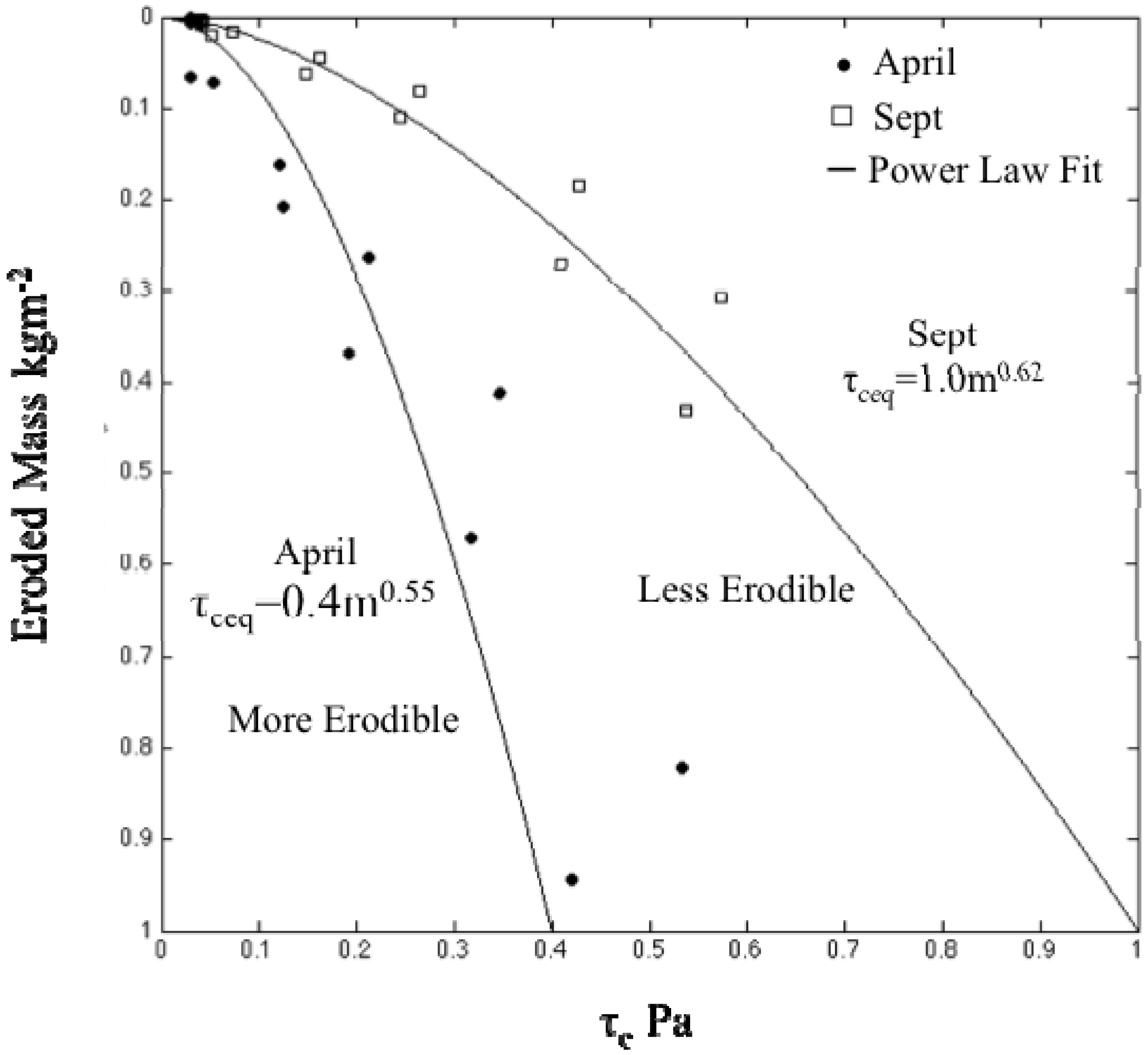
5.2. Sensitivity to τceq and τcinit

Power law fits to Gust microcosm data for the York River were used to define two depth-dependent critical shear stress profiles, τc (m), one based on cores collected in September 2007 and the second on cores collected in April 2007 [47] (Figure 2). Compared to the September data, the τc (m) profiles from April 2007 represented a time that had a more erodible seafloor. For the model runs described in this section, the same profiles were used for model initialization (τcinit) and to define the equilibrium toward which instantaneous profiles (τc) were nudged (τceq in Equation (2)). Results from two model simulations were compared to evaluate the sensitivity of model calculations to parameterization of the sediment bed’s critical shear stress profile. One used the power law fit to the September profile for both τcinit and τceq, while the second used the April profiles for both. Like the Standard Model, both assumed timescales for consolidation and swelling as Tc = 1 day and Ts = 25 days, but recall that the Standard Model used the April, more erodible, profile as τceq and the September, less erodible, profile for model initialization τcinit. A second set of these sensitivity tests used identical parameterization as the first two, except Ts = 50 days. The limits on computational time precluded doing additional tests such as a model using Ts = 2 days.
Figure 10 shows the calculated instantaneous τc profiles for the first two sensitivity tests, compared to the user-defined profiles of τceq and τcinit. When τceq and τcinit were defined using the September fit, the instantaneous τc profiles showed slight adjustment back to τceq (Figure 10a). This was not the case when τceq and τcinit were based on the more erodible April seabed (Figure 10b). Instead, the increased erodibility of the initial sediment bed provided a pool of easily resuspended material that when redeposited at slack tide, further increased the erodibility of the bed. With the consolidation timescale of one day, the instantaneous τc could not readjust to the equilibrium profile, τceq, but developed into an environment dominated by easily erodible, newly deposited sediment throughout the model run.
Figure 10. Daily instantaneous model calculated τc profiles (colored lines) shown with the profile used to parameterize these models (black lines). The equilibrium profile (τceq) and initial bed profile (τcrinit) were defined based on (a) September and (b) April profiles. Note: τceq = τcrinit for these model runs. The black arrows show the direction that Equation (2) will nudge the instantaneous τc toward the user-defined τceq.
Jmse 02 00413 g010
The increased erodibility of the second case led to a positive feedback between bed erodibility and sediment concentrations. This resulted in much higher estimated suspended-sediment concentrations than either the Standard Model or the case using the September profiles for both the equilibrium and initial values, as seen in the tidal phase averaged values (Figure 11). This result was insensitive to the swelling timescale used, which was not surprising because the modeled bed was always freshly deposited and thus easily erodible. Regardless of the defined Ts, concentrations estimated by the model simulation that defined τceq and τcinit based on the April fit exceeded the observed values by about 80–300 mg/L, while the model that used the September profiles provided much better estimates.

6. Discussion

This section first summarizes the model behavior for the York River case, and then discusses issues relating to model implementation and model parameters.

6.1. Summary of York River 3-D Hydrodynamic Cohesive Bed Model Performance

Implementation of the cohesive bed model in conjunction with the MUDBED field study provided a unique opportunity to evaluate model behavior both in terms of the system-wide feedbacks between bed erodibility and sediment concentration, and more specifically in comparison to field data from the MUDBED Intermediate site. Analyses of model results from July–August 2007 showed that the model represented trends in the spatial and temporal variability of bed erodibility and settling velocity observed in the York River estuary (Figure 4 and Figure 5).
Figure 11. Phase averaged concentration observed using the ADV, and estimated by model runs that defined (τceq) and (τcrinit) using the power law fits to the September and April profiles with swelling times of 50 and 25 days (see legend).
Jmse 02 00413 g011
Ongoing analysis of ADV data collected at the MUDBED Intermediate site during the summer of 2007 revealed that the variability in settling velocity and bed erodibility appear to fall into two regimes having distinct hydrodynamic and sediment characteristics [49]. Regime 1 represented periods dominated by easily suspended, slow settling flocculated muds, while Regime 2 represented periods strongly influenced by less easily suspended, faster settling, biologically repackaged fecal pellets mixed with flocs [49]. The analysis presented in this paper focused on a time classified as Regime 2.
Results from the three-dimensional York River Hydrodynamic Cohesive Bed model showed good agreement to field data from the observational period defined as Regime 2 [49], with only slight differences between model estimated and ADV observed bed stresses and bulk settling velocities (~18%). Though the model was biased towards higher bed stresses (Figure 6c) and higher settling velocities at peak flow, both model estimated and observed bulk settling velocities increased along with bed stress (Figure 7). This implied that differential resuspension of sediment types having the range of settling velocities considered in the model (0.8 to 2.4 mm/s) could account for the changes to settling velocity seen during a tidal cycle, without invoking aggregation and disaggregation processes. Looking more closely, the model overestimated bulk settling velocity as flow accelerated, with the biggest difference occurring at peak flow, which can be attributed to two things. First, the model only included two settling classes (0.8 mm/s and 2.4 mm/s), while suspended material in the York River estuary consists of many more particle types having a wide range of settling velocities [42,65]. Second, the model overestimated bed stresses throughout the tidal phase (Figure 6), which may have contributed to the overestimated concentrations (Figure 6b) as well as bulk settling velocities (Figure 7). Higher bed stresses were able to suspend a greater mass of material, including a greater amount of faster settling particles, which resulted in a higher estimate of bulk settling velocity [42]. Additionally the higher bed stresses would increase eddy diffusivity, mixing the more slowly settling material higher in the water column, and resulting in a greater fraction of faster settling material near the bed.
Though not shown in this paper, the model had less skill when applied to the period defined as Regime 1, overestimating the observed modeled bed stresses by 50%, while underestimating suspended-sediment concentrations by 17%. Field data imply that sediment-induced stratification more strongly influenced the system during Regime 1 than during Regime 2, and that stratification from both salinity and suspended-sediment gradients suppressed bed stresses during Regime 1 [49,61]. ROMS has the capacity to account for sediment induced stratification, but the process was neglected in this implementation. Future work will evaluate whether the turbulence closures in ROMS can represent sediment—induced stratification at the relevant vertical scales for the York River estuary, and whether including this process this improves the model skill during Regime 1.

6.2. Cohesive Bed Model Sensitivities

The cohesive bed model sensitivity tests done in this study explored the impact on estimated instantaneous critical stress profiles (τc) and suspended-sediment concentration to user-defined cohesive bed swelling time (Ts) and the initial and equilibrium τc profiles (τcinit and τceq). We did not examine sensitivity to the consolidation timescale, because it seemed better constrained in the literature than the swelling timescale [33,43].
Use of a short Ts allowed the instantaneous τc profiles to rapidly adjust to the equilibrium profile for a case where the system was less erodible than the equilibrium (Figure 8a). As Ts increased to 50 days, the adjustment of the instantaneous τc profiles became negligible (Figure 8c). Use of a shorter Ts resulted in a more erodible bed, which increased suspended-sediment concentrations in the water column (Figure 9). The sensitivity to Ts should be considered in the context of the model configuration, which for the Standard Model used a less erodible bed for initialization than for the equilibrium profile. The model simulation time, 120 days, included 90 days before the time period analyzed. When swelling timescale was long compared to the spin-up time, the model would be especially sensitive to the seabed initialization (i.e., τcinit). For example, using a Ts of 50 days meant that the instantaneous τc profiles would be especially sensitive to the initialization over the timescale considered by the model.
For the case where the model’s seabed was initialized to be especially erodible, however, positive feedbacks between sediment erodibility and concentrations led to the development of an even more erodible bed, and model estimates were then insensitive to Ts (Figure 10). This sensitivity test found that the model estimated instantaneous τc profiles and suspended-sediment concentrations were less sensitive to Ts than the profiles that were used to define τcinit and τceq (Figure 10 and Figure 11). We expect that the model estimates for this case would be more sensitive to Tc than Ts, but this was not evaluated directly, in part because the literature provides guidance for the consolidation timescales in the literature than the swelling timescales.
An important step in model implementation for the cohesive bed model was specification of both the initial and equilibrium critical stress profiles, and the consolidation and swelling timescales. The cohesive bed model is still fairly new, and a consensus for how the initial and equilibrium profiles should be defined has not been established. It is clear, however, that for a case where measured critical shear stress profiles exist, the model parameters, including both the initial and equilibrium profiles, should be defined so that instantaneous shear stress profiles usually remain within the realm of measured profiles. Additionally, the choice of erosion rate parameter (M) probably would influence model behavior and have implications for the suitability of different values of these parameters, but the value of M = 1 × 10⁻³ kg/(m2 s P) was not modified for this implementation from the value originally used by [54]. Each sensitivity test required significant computer time (a few days on our cluster), and full three-dimensional model runs were needed to evaluate system behavior under various parameter sets. For that reason, an exhaustive set of parameter choices was not explored, and we were limited to the cases discussed in section 5.2.
The availability of field observations from the MUDBED Intermediate site were valuable for constraining reasonable seabed profiles of critical shear stress, and water column estimates of bulk settling velocity and sediment concentration. In cases when field observations are unavailable, model estimates may reproduce realistic processes and trends, but should be analyzed with caution. Although this study offered much insight on implementing the cohesive bed model in a realistic environment, ongoing work is needed to further understand the use of the cohesive bed model in a complex system.

7. Conclusions

This study described the use of the CSTSMS cohesive bed model that accounts for erosion, deposition, consolidation and swelling in a three-dimensional hydrodynamic model to represent the York estuary, VA, USA. Results from a time period when sediment-induced stratification seemed to be unimportant showed good agreement with observations of sediment concentration, bed stress, and current velocity. The sensitivities of the cohesive model were explored by evaluating the impact on calculations of changes to the swelling timescale and the initial and equilibrium critical stress profiles, and model estimates were found to be sensitive to these parameters. The Standard Model was developed by choosing a swelling timescale and initial and equilibrium critical stress profiles for the York River three-dimensional model that showed good agreement with field observations of bed stress, current velocity, and sediment concentration using a tidal-phase averaged analysis. The model was able to capture observed spatial and temporal trends in settling velocity, and unlike previous models that did not allow for a depth varying τc this model was able to adequately represent feedbacks between erosion and deposition in a highly dynamic cohesive environment. The cohesive bed model is still fairly new, and more work is needed to determine how the initial and equilibrium profiles should be defined, especially in cases where observations are limited. However, results from this study demonstrate that this model promises to be a useful tool for investigating the fundamental controls on bed erodibility and settling velocity in the York River, a classical muddy estuary.

Acknowledgments

Funding by the National Science Foundation (OCE-1061781 and OCE-0536572) supported Fall, Harris, Friedrichs, and Rinehimer. Lindsey Kraatz (formerly VIMS) contributed to some of the model runs. The authors appreciate discussions with Linda Schaffner, Marjorie Friedrichs (both VIMS) and Larry Sanford (U. Maryland Center for Environmental Science), who aided model development. Comments from Patrick Dickhudt (U.S. Geological Survey) improved an earlier version of this paper. Use of trade, product, or firm names is for descriptive purposes only and does not imply endorsement by the U.S. Government. This is contribution number 3363 of the Virginia Institute of Marine Science, College of William & Mary.

Author Contributions

K.A. Fall completed model runs and data analysis. She drafted the manuscript, which the co-authors then edited. C.K. Harris supervised the model runs and analysis. C.T. Friedrichs supervised the data analysis. J.P. Rinehimer initially implemented the model for the York River. C.R. Sherwood oversaw changes to the model source code to include the cohesive bed formulation.

Conflicts of Interest

The authors declare no conflicts of interest.

References

  1. Winterwerp, J.C.; Van Kesteren, W.G. Introduction to the Physics of Cohesive Sediment Dynamics in the Marine Environment; Elsevier: Amsterdam, The Netherlands, 2004. [Google Scholar]
  2. Reay, W.G. Water quality within the York River estuary. J. Coast. Res. 2009, 25, 23–39. [Google Scholar] [CrossRef]
  3. Sanford, L.; Chang, M. The bottom boundary condition for suspended sediment deposition. J. Coast. Res. 1997, 13, 3–17. [Google Scholar]
  4. Friedrichs, C.T.; Cartwright, G.M.; Dickhudt, P.J. Quantifying benthic exchange of fine sediment via continuous, noninvasive measurements of settling velocity and bed erodibility. Oceanography 2008, 21, 168–172. [Google Scholar] [CrossRef]
  5. Harris, C.K.; Sherwood, C.R.; Signell, R.P.; Bever, A.J.; Warner, J.C. Sediment dispersal in the northwestern Adriatic Sea. J. Geophys. Res. Oceans 2008, 113. [Google Scholar] [CrossRef]
  6. Gong, W.; Shen, J. Response of sediment dynamics in the York River Estuary, USA to tropical cyclone Isabel of 2003. Estuar. Coast. Shelf Sci. 2009, 84, 61–74. [Google Scholar] [CrossRef]
  7. Gong, W.; Shen, J. A model diagnostic study of age of river-borne sediment transport in the tidal York River Estuary. Environ. Fluid Mech. 2010, 10, 177–196. [Google Scholar] [CrossRef]
  8. Fugate, D.C.; Friedrichs, C.T. Controls on suspended aggregate size in partially mixed estuaries. Estuar. Coast. Shelf Sci. 2003, 58, 389–404. [Google Scholar] [CrossRef]
  9. Scully, M.E.; Friedrichs, C.T. The influence of asymmetries in overlying stratification on near-bed turbulence and sediment suspension in a partially mixed estuary. Ocean Dyn. 2003, 53, 208–219. [Google Scholar] [CrossRef]
  10. Cartwright, G.M.; Friedrichs, C.T.; Dickhudt, P.J.; Gass, T.; Farmer, F.H. Using the acoustic doppler velocimeter (ADV) in the MUDBED real-time observing system. In Marine Technology for Our Future: Global and Local Challenges, Proceedings of OCEANS 2009, MTS/IEEE Biloxi, Gloucester, VA, USA, 1–9 November 2009.
  11. Dickhudt, P.J.; Friedrichs, C.T.; Schaffner, L.C.; Sanford, L.P. Spatial and temporal variation in cohesive sediment erodibility in the York River estuary, eastern USA: A biologically influenced equilibrium modified by seasonal deposition. Mar. Geol. 2009, 267, 128–140. [Google Scholar] [CrossRef]
  12. Amos, C.L.; Umgiesser, G.; Ferrarin, C.; Thompson, C.; Whitehouse, R.; Sutherland, T.; Bergamasco, A. The erosion rates of cohesive sediments in Venice Lagoon, Italy. Cont. Shelf Res. 2010, 30, 859–870. [Google Scholar] [CrossRef]
  13. Postma, H. Sediment transport and sedimentation in the estuarine environment. Am. Assoc. Adv. Sci. 1967, 83, 158–179. [Google Scholar]
  14. Schubel, J.R. Turbidity maximum of the northern Chesapeake Bay. Science 1968, 161, 1013–1015. [Google Scholar] [CrossRef]
  15. Dyer, K.R. Sediment transport processes in estuaries. Dev. Sedimentol. 1995, 53, 423–449. [Google Scholar] [CrossRef]
  16. Geyer, W.R. The importance of suppression of turbulence by stratification on the estuarine turbidity maximum. Estuaries 1993, 16, 113–125. [Google Scholar] [CrossRef]
  17. Jay, D.A.; Musiak, J.D. Particle trapping in estuarine tidal flows. J. Geophys. Res. Oceans 1994, 99, 20445–20461. [Google Scholar] [CrossRef]
  18. Scully, M.E.; Friedrichs, C.T. Sediment pumping by tidal asymmetry in a partially mixed estuary. J. Geophys. Res. 2007, 112. [Google Scholar] [CrossRef]
  19. Schoellhamer, D. Influence of salinity, bottom topography, and tides on locations of estuarine turbidity maxima in northern San Francisco Bay. In Coastal and Estuarine Fine Sediment Transport Processes; McAnally, W.H., Mehta, A.J., Eds.; Elsevier: Amsterdam, The Netherlands, 2001; pp. 343–357. [Google Scholar]
  20. Lin, J.; Kuo, A.Y. Secondary turbidity maximum in a partially mixed microtidal estuary. Estuaries 2001, 24, 707–720. [Google Scholar] [CrossRef]
  21. Woodruff, J.D.; Geyer, W.R.; Sommerfield, C.K.; Driscoll, N.W. Seasonal variation of sediment deposition in the Hudson River Estuary. Mar. Geol. 2001, 179, 105–119. [Google Scholar] [CrossRef]
  22. Ralston, D.K.; Warner, J.C.; Geyer, W.R.; Wall, G.R. Sediment transport due to extreme events: The Hudson River Estuary after tropical storms Irene and Lee. Geophys. Res. Lett. 2013, 40, 5451–5455. [Google Scholar] [CrossRef]
  23. Shields, A.; California Institute of Technology, Pasadena, CA, USA. Application of Similarity Principles and Turbulence Research to Bed-Load Movement. Unpublished work. 1936. [Google Scholar]
  24. Parchure, T.M.; Mehta, A.J. Erosion of soft cohesive sediment deposits. J. Hydraul. Eng. 1985, 111, 1308–1326. [Google Scholar] [CrossRef]
  25. Amos, C.L.; Daborn, G.; Christian, H.; Atkinson, A.; Robertson, A. In situ erosion measurements on fine-grained sediments from the Bay of Fundy. Mar. Geol. 1992, 108, 175–196. [Google Scholar] [CrossRef]
  26. Maa, J.P.; Sanford, L.; Halka, J.P. Sediment resuspension characteristics in Baltimore Harbor, Maryland. Mar. Geol. 1998, 146, 137–145. [Google Scholar] [CrossRef]
  27. Roberts, J.; Jepsen, R.; Gotthard, D.; Lick, W. Effects of particle size and bulk density on erosion of quartz particles. J. Hydraul. Eng. 1998, 124, 1261–1267. [Google Scholar]
  28. Ariathurai, C.R.; Krone, R.B. Finite element model for cohesive sediment transport. J. Hydraul. Div. 1976, 102, 323–338. [Google Scholar]
  29. McLean, S.R. Theoretical modelling of deep ocean sediment transport. Mar. Geol. 1985, 66, 243–265. [Google Scholar] [CrossRef]
  30. Andersen, T. Seasonal variation in erodibility of two temperate, microtidal mudflats. Estuar. Coast. Shelf Sci. 2001, 53, 1–12. [Google Scholar] [CrossRef]
  31. Sanford, L.P.; Maa, J.P. A unified erosion formulation for fine sediments. Mar. Geol. 2001, 179, 9–23. [Google Scholar] [CrossRef]
  32. Sanford, L.P. Uncertainties in sediment erodibility estimates due to a lack of standards for experimental protocols and data interpretation. Int. Environ. Assess. Manag. 2006, 2, 29–34. [Google Scholar] [CrossRef]
  33. Rinehimer, J.P.; Harris, C.K.; Sherwood, C.R.; Sanford, L.P. Estimating cohesive sediment erosion and consolidation in a muddy, tidally-dominated environment: Model behavior and sensitivity. In Proceedings of 10th Estuarine and Coastal Modeling, Reston, VA, USA, 5–7 November 2008; American Society of Civil Engineers: Reston, VA, USA, 2008; pp. 819–838. [Google Scholar]
  34. Wang, X.; Pinardi, N. Modeling the dynamics of sediment transport and resuspension in the northern Adriatic Sea. J. Geophys. Res. 2002, 107. [Google Scholar] [CrossRef]
  35. Lin, J.; Kuo, A.Y. A model study of turbidity maxima in the York River Estuary, Virginia. Estuaries 2003, 26, 1269–1280. [Google Scholar] [CrossRef]
  36. Harris, C.K.; Traykovski, P.A.; Geyer, W.R. Flood dispersal and deposition by nearbed gravitational sediment flows and oceanographic transport: A numerical modeling study of the Eel River Shelf, Northern California. J. Geophys. Res. Oceans 2005, 110. [Google Scholar] [CrossRef]
  37. Geyer, W.R.; Woodruff, J.D.; Traykovski, P. Sediment transport and trapping in the Hudson River Estuary. Estuaries 2001, 24, 670–679. [Google Scholar]
  38. Harris, C.K.; Wiberg, P.L. A two-dimensional, time-dependent model of suspended sediment transport and bed reworking for continental shelves. Comput. Geosci. 2001, 27, 675–690. [Google Scholar] [CrossRef]
  39. Sanford, L.P.; Suttles, S.E.; Halka, J.P. Reconsidering the physics of the Chesapeake Bay estuarine turbidity maximum. Estuaries 2001, 24, 655–669. [Google Scholar]
  40. Stevens, A.; Wheatcroft, R.; Wiberg, P. Seabed properties and sediment erodibility along the western Adriatic margin, Italy. Cont. Shelf Res. 2007, 27, 400–416. [Google Scholar] [CrossRef]
  41. Kwon, J.-I. Simulation of Turbidity Maximums in the York River, Virginia. Ph.D. Thesis, School of Marine Science, College of William and Mary, Gloucester Point, VA, USA, June 2005. [Google Scholar]
  42. Cartwright, G.; Friedrichs, C.; Sanford, L. In situ characterization of estuarine suspended sediment in the presence of muddy flocs and pellets. In Proceedings of Coastal Sediments, Miami, FL, USA, 2–6 May 2011; pp. 642–655.
  43. Sanford, L.P. Modeling a dynamically varying mixed sediment bed with erosion, deposition, bioturbation, consolidation, and armoring. Comput. Geosci. 2008, 34, 1263–1283. [Google Scholar] [CrossRef]
  44. Friedrichs, C.T. York River physical oceanography and sediment transport. J. Coast. Res. 2009, 25, 17–22. [Google Scholar] [CrossRef]
  45. Schaffner, L.C.; Dellapenna, T.M.; Hinchey, E.K.; Friedrichs, C.T.; Thompson Neubauer, M.; Smith, M.E.; Kuehl, S.A. Physical energy regimes, seabed dynamics and organism-sediment interactions along an estuarine gradient. In Organism-Sediment Interactions; Aller, J.Y., Woodin, S.A., Aller, R.C., Eds.; University of South Carolina Press: Columbia, SC, USA, 2001. [Google Scholar]
  46. Dellapenna, T.M.; Kuehl, S.A.; Schaffner, L.C. Ephemeral deposition, seabed mixing and fine-scale strata formation in the York River Estuary, Chesapeake Bay. Estuar. Coast. Shelf Sci. 2003, 58, 621–643. [Google Scholar] [CrossRef]
  47. Maa, J.P.; Kim, S. A constant erosion rate model for fine sediment in the York River, Virginia. Environ. Fluid Mech. 2001, 1, 345–360. [Google Scholar] [CrossRef]
  48. Dickhudt, P.J. Controls on Erodibility in a Partially Mixed Estuary: York River, Virginia. Master’s Thesis, School of Marine Science, College of William and Mary, Gloucester Point, VA, USA, July 2008. [Google Scholar]
  49. Fall, K.A.; Friedrichs, C.T.; Cartwright, G.M. Controls on Particle Settling Velocity and Bed Erodibility in the Presence of Muddy Flocs and Pellets as Inferred by ADVs, York River Estuary, Virginia, USA. Ocean Dyn. 2014; to be submitted for publication. [Google Scholar]
  50. Uncles, R.; Stephens, J. Distributions of suspended sediment at high water in a macrotidal estuary. J. Geophys. Res. 1989, 94, 14395–14405. [Google Scholar] [CrossRef]
  51. Shchepetkin, A.F.; McWilliams, J.C. The regional oceanic modeling system (ROMS): A split-explicit, free-surface, topography-following-coordinate oceanic model. Ocean Model. 2005, 9, 347–404. [Google Scholar] [CrossRef]
  52. Haidvogel, D.B.; Arango, H.; Budgell, W.; Cornuelle, B.; Curchitser, E.; Di Lorenzo, E.; Lanerolle, L. Ocean forecasting in terrain-following coordinates: Formulation and skill assessment of the regional ocean modeling system. J. Comput. Phys. 2008, 227, 3595–3624. [Google Scholar] [CrossRef]
  53. Warner, J.C.; Sherwood, C.R.; Signell, R.P.; Harris, C.K.; Arango, H.G. Development of a three-dimensional, regional, coupled wave, current, and sediment-transport model. Comput. Geosci. 2008, 34, 1284–1306. [Google Scholar] [CrossRef]
  54. Rinehimer, J.P. Sediment Transport and Erodibility in the York River Estuary: A Model Study. Master’s Thesis, School of Marine Science, College of William and Mary, Gloucester Point, VA, USA, October 2008. [Google Scholar]
  55. Mellor, G.L.; Yamada, T. Development of a turbulence closure model for geophysical fluid problems. Rev. Geophys. 1982, 20, 851–875. [Google Scholar] [CrossRef]
  56. Smolarkiewicz, P.K.; Margolin, L.G. MPDATA: A finite-difference solver for geophysical flows. J. Comput. Phys. 1998, 140, 459–480. [Google Scholar] [CrossRef]
  57. Warner, J.C.; Geyer, W.R.; Lerczak, J.C. Numerical modeling of an estuary: A comprehensive skill assessment. J. Geophys. Res. 2005, 110. [Google Scholar] [CrossRef]
  58. Sherwood, C.R.; Aretzabaleta, A.; Harris, C.K.; Rinehimer, J.P.; Ferre, B.; Veraney, R. Extension of the Community Sediment Transport Modeling System for Coheisve Sediment: Floc and Muddy Bed Dynamics. 2014; to be submitted for publication. [Google Scholar]
  59. USGS Water Data Website. Available online: http://waterdata.usgs.gov/nwis (accessed on 10 May 2010).
  60. Chesapeake Bay Program Data Hub Website. Available online: http://www.chesapeakebay.net/data (accessed on 26 February 2010).
  61. Fugate, D.C.; Friedrichs, C.T. Determining concentration and fall velocity of estuarine particle populations using ADV, OBS and LISST. Cont. Shelf Res. 2002, 22, 1867–1886. [Google Scholar] [CrossRef]
  62. Friedrichs, C.; Wright, L.; Hepworth, D.; Kim, S. Bottom-boundary-layer processes associated with fine sediment accumulation in coastal seas and bays. Cont. Shelf Res. 2000, 20, 807–841. [Google Scholar] [CrossRef]
  63. Dyer, K. Coastal and Estuarine Sediment Dynamics; Wiley: Chichester, UK, 1986. [Google Scholar]
  64. Kraatz, L.M.; Friedrichs, C.T.; Cartwright, G.M.; Fall, K.A.; Wilkerson, C.N. Relationships between erodibility and fine-grained sea bed properties on tidal to seasonal time-scales, York River Estuary, Virginia, USA. In Proceedings of Physics of Estuaries and Coastal Seas, 16th International Biennial Conference, New York, NY, USA, 12–16 August 2012.
  65. Cartwright, G.M.; Friedrichs, C.T.; Smith, S.J. A test of the ADV-based Reynolds flux method for in situ estimation of sediment settling velocity in a muddy estuary. Geo-Mar. Lett. 2013, 33, 477–484. [Google Scholar] [CrossRef]

