Article

Machine Learning for Wind Pattern Estimation at Data-Scarce Coastal Ports: A Comparative Study Using Real Measurements

by
Anastasios Giannopoulos
1,*,
Aikaterini Karditsa
1,
Maria Hatzaki
2 and
Panagiotis Trakadas
1
1
Department of Ports Management and Shipping, National and Kapodistrian University of Athens, Evripus Campus, 34400 Euboea, Greece
2
Department of Geology and Geoenvironment, National and Kapodistrian University of Athens, 15771 Athens, Greece
*
Author to whom correspondence should be addressed.
J. Mar. Sci. Eng. 2025, 13(12), 2375; https://doi.org/10.3390/jmse13122375
Submission received: 17 November 2025 / Revised: 10 December 2025 / Accepted: 12 December 2025 / Published: 15 December 2025
(This article belongs to the Section Coastal Engineering)

Abstract

Accurate wind information is essential for safe and efficient port operations, yet many small and medium-sized coastal ports lack dense meteorological instrumentation. This paper presents a data-driven framework for wind speed prediction at such ports by leveraging long-term historical measurements from nearby reference stations. Focusing on a real-world case study at the Chalkida port in Greece, the framework integrates both deterministic and Machine Learning (ML) models trained on historical wind patterns of archived wind data from four surrounding locations. We examine both short- and long-horizon prediction periods, using recently acquired wind measurements at the target port for model validation. Deterministic baselines include simple and weighted averaging schemes, while supervised ML methods, such as Multiple Linear Regression, Decision Trees, Support Vector Regression, Random Forests, and Gradient Boosting, are trained to capture complex spatiotemporal patterns. Experimental results highlight that ensemble-based ML models, particularly Gradient Boosting, achieve superior accuracy in short-term forecasting, while the optimal predictor varies with the forecast horizon. The proposed approach enables the deployment of virtual wind stations in data-scarce ports and can be periodically updated to dynamically select the most suitable model, thereby supporting climate adaptation strategies, localized wind monitoring, and operational planning without requiring dense local instrumentation.

1. Introduction

Coastal ports play a central role in global trade, logistics, and economic development, acting as critical gateways for the transportation of goods and passengers [1,2]. However, these infrastructures are increasingly exposed to the adverse effects of climate change, including rising sea levels, intensified storms, and changes in wind regimes [3]. Among these, wind events pose a particularly immediate and operationally disruptive threat [4]. Sudden gusts, directional shifts, or prolonged high winds can delay ship docking and unloading, damage port equipment, disrupt container stacking, or even endanger human lives [5]. Moreover, wind conditions strongly affect emissions dispersion, mooring forces, and the scheduling of offshore activities such as maintenance of coastal structures or energy harvesting systems [6]. Therefore, the availability of accurate and timely wind data is not only crucial for daily operations but also for strategic planning toward climate resilience and adaptation.
Despite the increasing demand for high-resolution meteorological data, many small and medium-sized ports remain under-equipped with permanent and high-frequency monitoring systems. The installation and maintenance of meteorological stations, especially those capable of long-term wind recording at multiple heights and locations, can be financially or logistically prohibitive [7]. As a result, port authorities often lack reliable, localized data to inform operational decisions or model future climate scenarios. In this context, reanalysis datasets, such as ERA5, corresponding to the fifth generation European Centre for Medium-Range Weather Forecasts (ECMWF) reanalysis for the global climate and weather for the past 8 decades (provided by the Copernicus Climate Change Service), offer a globally available and long-term source of wind data [8,9]. However, these datasets typically represent broader spatial scales and may not fully capture the local microclimates and topographic influences found in port environments. Consequently, there exists a pressing need to develop techniques that can infer or reconstruct accurate wind profiles at data-scarce coastal ports by leveraging spatially and temporally aligned information from surrounding locations [10,11]. The concept of data augmentation for high spatial resolution meteorological monitoring is depicted in Figure 1. This schematic illustration is conceptual to introduce virtual monitoring via Machine Learning (ML) and does not represent actual geographic locations or elevations. Its aim is to visualize the high-level concept of using ML-based estimation to emulate high-resolution wind measurements via virtual stations, leveraging sparse reference points.
The proposed approach introduces several methodological aspects that are currently limited or under-studied in wind estimation literature. First, it enables the estimation of wind conditions at ports lacking dense instrumentation by leveraging long-term spatiotemporal correlations from reference datasets. Second, it introduces a virtual station construction method using ML models trained on seasonally matched ERA5 data, eliminating the need for extensive local historical measurements. Third, it combines deterministic and ML-based models into a unified comparative framework validated with real pilot measurements. Based on these contributions, the present study proposes a generalizable and adaptable alternative to traditional downscaling or sensor-intensive approaches.
The primary objective of this study is to investigate the feasibility and accuracy of reconstructing wind patterns at under-monitored ports using long-term wind recordings from nearby reference sites [12]. Focusing on a real-world case study, the Greek port of Chalkida in Central Evoia, we develop a methodology that utilizes ERA5 reanalysis data from four neighboring offshore or coastal grid points spanning the period from 1970 to 2024 [13]. These reference locations serve as the basis for estimating the wind conditions at the Chalkida port during (i) a recent 11-day period (20–31 December 2023) and (ii) longer-horizon 8-months (29 February–16 October 2024), for which real in situ wind measurements are available through a meteorological station deployed in the port. The estimation task involves predicting key wind variables (timeseries of u10 and v10 wind coordinates, and wide speed) at the target location based on spatiotemporal features extracted from the reference points.
To address this estimation task, we explore and systematically compare a broad set of models, ranging from deterministic approaches to machine learning-based regressors. Specifically, we design and implement four deterministic baseline models, including simple and weighted averaging variants that incorporate cross-location correlation scores [14]. These are contrasted against five machine learning models, including Multiple Linear Regression (MLR), Decision Tree Regression (DTR), Support Vector Regression (SVR), Random Forest Regression (RFR), and Gradient Boosting Regression (GBR) [15,16,17]. All models are trained using a unique proposed spatiotemporal methodology that matches hourly timestamps across years (i.e., the same day and hour of each year) to extract seasonally relevant training samples.
The main contributions of this work can be summarized as follows:
  • We propose a unified, generalizable and multi-model framework for wind speed estimation in data-scarce coastal ports, integrating both deterministic statistical models and ML algorithms. This framework allows for the deployment of virtual wind stations where dense meteorological instrumentation is unavailable.
  • We design a spatiotemporal data extraction and alignment methodology, which utilizes over five decades of hourly ERA5 reanalysis data from surrounding reference locations. By aggregating data across years for the same day and hour, we capture non-linear and recurring seasonal wind patterns that enrich the model training process.
  • We implement and compare a set of deterministic models (e.g., simple averaging, correlation-weighted averaging) with five supervised ML models to assess their performance across different prediction horizons.
  • Through extensive validation using real in situ wind speed measurements at the pilot port (Chalkida, Greece), we demonstrate that ensemble-based ML models, particularly GBR, offer significantly improved prediction accuracy in short-term forecasting scenarios. In long-term predictions, simpler tree-based models such as DTR remain competitive due to their lower variance and robustness to overfitting.
  • Finally, we show that the proposed methodology is not tied to a specific model but can be periodically retrained and adapted to new data, enabling dynamic selection of the best-performing predictor depending on the forecasting horizon and environmental conditions.
The proposed framework is generalizable and may serve as a practical data-driven solution for wind pattern estimation in under-monitored coastal environments, supporting port authorities in operational decision-making, risk management, and climate resilience planning without requiring expensive infrastructure investments.

2. Related Work

2.1. Wind Data Downscaling and Interpolation Techniques

Downscaling and spatial interpolation techniques have long been used to improve the spatial resolution of meteorological data in applications where direct measurements are sparse or absent [18]. Traditional approaches include deterministic interpolation methods such as Inverse Distance Weighting (IDW), Kriging, and spline-based techniques, which estimate unknown values by leveraging spatial autocorrelation among neighboring stations [19,20]. While these methods are computationally efficient and easy to implement, they often struggle to capture non-linear terrain influences, especially in complex coastal environments where land–sea interactions and topographic heterogeneity can significantly distort local wind fields.
To overcome these limitations, physical downscaling methods such as dynamical modeling have been employed. These methods use nested atmospheric models (e.g., WRF or MM5) that simulate local-scale meteorological conditions based on large-scale inputs [21,22]. Although more accurate in theory, such models require extensive computational resources, domain-specific parameter tuning, and boundary conditions, making them less suitable for real-time or scalable deployment in small ports. Consequently, hybrid approaches combining physical modeling with statistical or data-driven post-processing have emerged, attempting to balance physical realism with operational efficiency [23]. Nonetheless, the integration of domain knowledge and spatiotemporal patterns into downscaling models remains an active research challenge, particularly for wind estimation in under-instrumented maritime environments.

2.2. Machine Learning in Meteorology

In recent years, machine learning (ML) and deep learning (DL) models have gained substantial traction in the meteorological community for forecasting and reconstruction tasks [24,25,26]. ML models can learn complex, nonlinear relationships between inputs and outputs directly from historical data without requiring explicit physical formulations [27]. Algorithms such as Support Vector Machines (SVM), Random Forests (RF), Gradient Boosting Machines (GBM), and Artificial Neural Networks (ANNs) have been successfully applied in forecasting wind speed, solar radiation, temperature, and precipitation, often outperforming traditional numerical models in short-term prediction accuracy [28].
A key advantage of ML approaches is their adaptability to diverse spatial and temporal resolutions, making them particularly useful in data-scarce scenarios. For instance, when observations are available only from surrounding locations, ML models can be trained to interpolate or infer missing values at the target site using correlated variables. More advanced architectures such as Convolutional Neural Networks (CNNs) and Long Short-Term Memory (LSTM) networks have also been applied to capture spatial dependencies and temporal dynamics, respectively, though they often require large and well-structured datasets [29,30]. In the context of wind estimation, studies have explored both pure time-series models and spatiotemporal predictors combining neighboring stations, terrain data, and meteorological features [31]. However, much of this work focuses on inland wind farms or urban environments, with limited application in coastal port regions where data sparsity and sea–land interactions pose unique modeling challenges.

2.3. ERA5 Reanalysis Applications

Reanalysis datasets such as ERA5, produced by the Copernicus Climate Change Service, provide consistent, gap-free atmospheric data at global scale and hourly resolution [32]. ERA5 assimilates a wide range of satellite and in situ observations into a physics-based numerical model to generate temporally and spatially complete weather fields, including 10-meter wind components (u10, v10), temperature, pressure, and other variables. Due to their long historical coverage (1970–present) and fine temporal granularity, ERA5 datasets have become a valuable resource for climate diagnostics, model training, and retrospective analysis [8,9].
Numerous studies have leveraged ERA5 data to support coastal and offshore wind resource assessment, validate satellite retrievals, and initialize regional climate models [33]. More recently, ERA5 has been used in data-driven workflows to reconstruct missing measurements, especially in oceanic or rural regions where ground-based stations are sparse [34,35]. However, while ERA5 captures synoptic-scale patterns effectively, it may underrepresent local phenomena such as orographic acceleration, land–sea breezes, or port-specific microclimates due to its coarse spatial resolution (30 km grid) [36]. Therefore, ERA5 is increasingly integrated into hybrid systems where machine learning or statistical post-processing refines the data for local applications. In this study, we build on this paradigm by using multi-decade ERA5 data from reference grid points to estimate short-term wind conditions at a nearby port lacking long-term instrumentation.

2.4. Existing Gaps in Wind Prediction for Data-Scarce Ports

Despite the substantial progress in both physical downscaling techniques and machine learning applications for meteorological forecasting, existing approaches often fall short in operationally constrained and data-scarce environments such as small and medium-sized coastal ports [37]. Traditional interpolation and reanalysis-based estimations fail to account for fine-scale local effects without in situ calibration, while most machine learning studies either focus on fully instrumented inland regions or rely on long-term historical records at the target site, data that are frequently unavailable for minor ports [38]. Furthermore, very few studies systematically evaluate and compare deterministic and machine learning models using long-term multi-source datasets to estimate wind patterns at under-monitored maritime locations. This creates a methodological and practical gap in the literature: how can we accurately estimate local wind conditions using only long-term data from nearby reference points, without relying on direct historical records from the port of interest?
Addressing this gap, our study proposes a unified framework for wind pattern estimation at data-scarce coastal ports, combining deterministic baselines with supervised learning models trained on spatiotemporally aligned ERA5 data. By incorporating both short-term real-world measurements and multi-decade historical records from neighboring sites, we provide a reproducible and scalable approach that supports resilient port operations without requiring dense local meteorological instrumentation.

3. Materials and Methods

3.1. Telemetry System Installation at the Pilot Port

To support real-time and offline wind analysis at the pilot port, a dedicated telemetry infrastructure was deployed, enabling continuous environmental monitoring and remote data accessibility. The overall setup is depicted in Figure 2.
A professional-grade meteorological station was installed on-site to record atmospheric and sea-related parameters, including wind speed and direction, temperature, and humidity. Measurements were exported in semi-hourly intervals and stored locally in a recording file. The station was connected to a Raspberry Pi 4 microserver, which ran a control program to ensure automated collection, basic pre-processing, and structured archiving of the accumulated data. To ensure data safety and facilitate further analysis, two parallel storage operations were implemented: (i) creation of a local backup file, and (ii) compilation of a cumulative data file in standardized format. The latter was periodically uploaded via a Python (Release 3.11.9) script using the Google Sheets API, allowing seamless integration with a cloud-based spreadsheet service.
Processed time series were automatically visualized using pre-defined graph templates that capture temporal variations in atmospheric and oceanographic conditions. These visualizations were embedded in a website through the publication of dynamic auto-updating HTML elements, enabling open access to near real-time telemetry data. Remote offline analysis is finally performed as described in the next sections.

3.2. Dataset and Preprocessing

3.2.1. Data Sources

To address the challenge of wind pattern estimation in data-scarce coastal regions, this study utilizes both historical (reanalysis) and real sensor data spanning multiple temporal resolutions. Specifically, wind data from four ERA5 reanalysis reference locations situated near the port of Chalkida were extracted from 1 January 1970 to 31 December 2024, with hourly temporal granularity. The four ERA5 reference locations were selected based on their geographic proximity to the target port and their ability to spatially enclose it from multiple directions (north, east, south, and west), ensuring representative coverage of the main wind inflow pathways in the broader coastal and marine region. These reference points, strategically selected to surround the target port, offer a long-term historical context and serve as the basis for reconstructing wind dynamics at the Location of Interest (LoI), namely the Greek Port of Chalkida. The historical wind data were retrieved from the standard ERA5 reanalysis dataset provided by the Copernicus Climate Data Store, with a spatial resolution of 0.25° (approximately 27.7 km). This dataset includes global hourly wind components at 10 m above ground level. Note that we did not use the ERA5-Land dataset, which offers a finer resolution (11 km) but is limited to land-only variables and lacks near real-time updates. Nonetheless, the proposed methodology is agnostic to the dataset granularity and is equally applicable to other datasets such as ERA5-Land. Hence, although we use typical ERA5 data, the goal is to build machine-learning-based virtual stations that reconstruct the localized behavior of any reanalysis grid point using surrounding spatial information and observed short-term ground truth data.
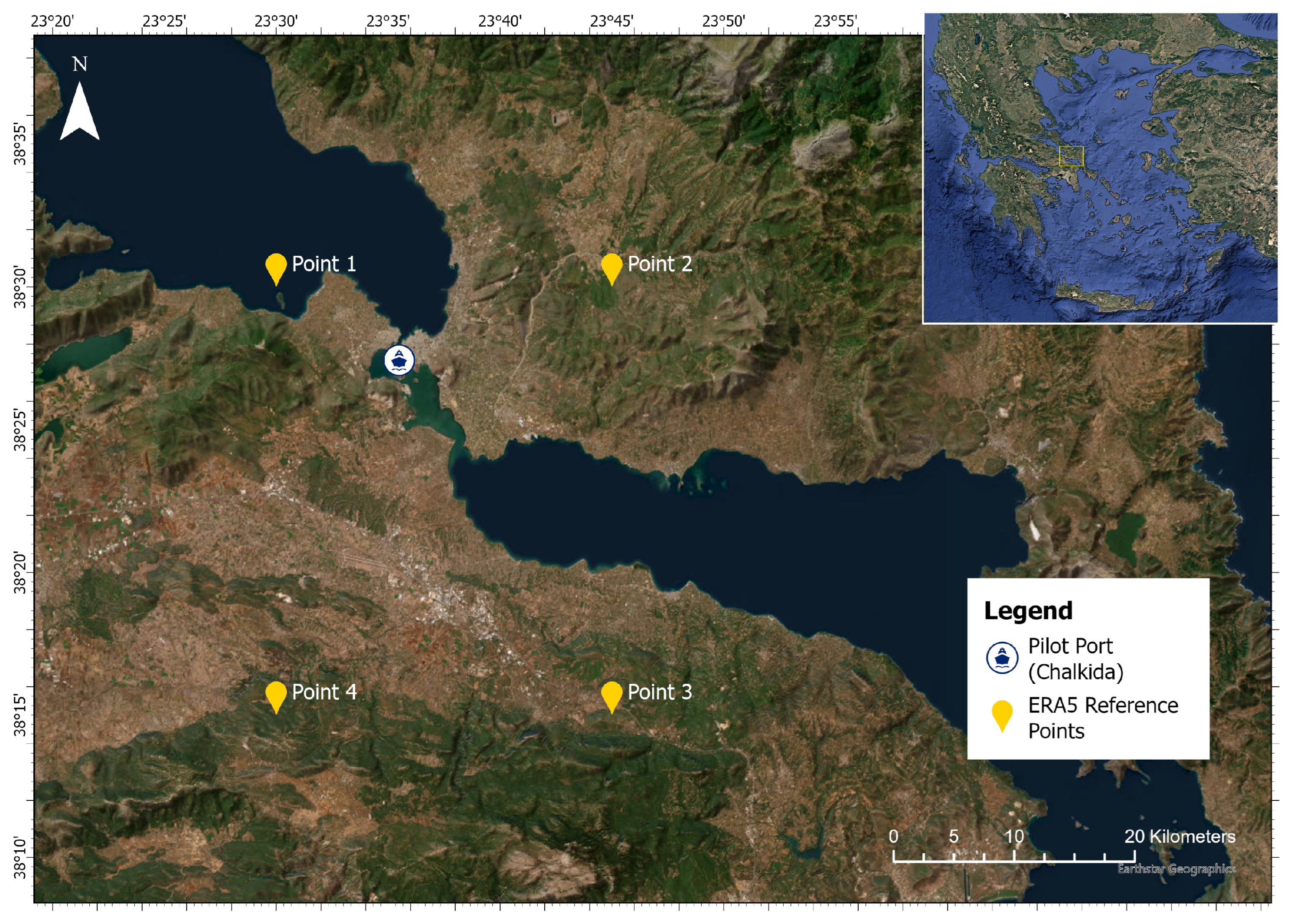
A summary of the ERA5 dataset information is described in Table 1, while the location topology of the four reference points and the pilot port is depicted in Figure 3. Figure 3 provides the actual spatial distribution of the ERA5 reference locations and the Chalkida port target station using a real topographic background. It is notable that the terrain effects are implicitly embedded in the historical data used for training, and thus are indirectly captured by the data-driven models.
In addition to reanalysis data, ground truth measurements were obtained from a physical meteorological sensor installed at the LoI. These measurements cover two distinct periods:
  • Short-term Period: From 20 December to 31 December 2023;
  • Long-term Period: From 26 February to 29 October 2024.
These real measurements enable model calibration and validation, ensuring realistic performance evaluation.

3.2.2. Variables of Interest

At each data point (ERA5 and real sensors), the following variables were recorded: (i) u 10 wind component, reflecting eastward wind component at 10 m (in m/s), and (ii) v 10 wind component, representing northward wind component at 10 m (in m/s). From these components, the wind speed u ( t ) at each time point t was derived as:
u ( t ) = u 10 2 ( t ) + v 10 2 ( t )
The wind direction θ ( t ) was computed as:
θ ( t ) = arctan v 10 ( t ) u 10 ( t ) · 180 π
normalized to the range [0°, 360°]. This transformation enabled the generation of polar representations (wind rose plots), trend estimation, and spatial correlation analyses across regions (see Section 3.3).

3.2.3. Preprocessing Steps

Prior to modeling, a comprehensive preprocessing pipeline was executed. The following steps were implemented:
1.
Timestamp Harmonization: ERA5 timestamps in Greek-formatted strings were converted to ISO-standard 24 h date–time format, ensuring consistent temporal indexing across all datasets.
2.
Variable Transformation: Wind speed and direction were computed from the u 10 and v 10 components at every time point for all locations.
3.
Temporal Alignment: All datasets (ERA5 and target sensor) were aligned based on the exact hour, day, and month to allow fair comparison across years and locations. To ensure uniformity in time indexing, all ERA5 datasets were inherently recorded at hourly resolution (i.e., on the hour: 00:00, 01:00, …, 23:00). On the other hand, the Chalkida port telemetry station records measurements every 30 min (e.g., 00:00, 00:30, 01:00, etc.). To harmonize the datasets for analysis, we retained only the Chalkida measurements that exactly matched the ERA5 timestamps (specifically, those recorded at full hours), thereby discarding the intermediate half-hour values. This alignment step ensured that all reference and target data points were perfectly synchronized on an hourly basis.
4.
Seasonal Subset Extraction: For model training and evaluation, specific periods of interest were isolated. Specifically, the short-term evaluation window (form 20 December 2023 to 31 December 2023) and the long-term evaluation window (from 26 February 2024 to 29 October 2024) were extracted from all 54 years of ERA5 data to construct matching historical subsets. These subsets capture interannual variability while preserving daily characteristics.
5.
3D Matrix Reshaping: A 3-dimensional matrix was constructed with dimensions [ L × T × Y ] , where L = 4 reference locations, T are the hourly time steps (separately for the two periods of interest), Y is the years. This matrix allowed model-specific extraction of historical patterns, year-wise averaging, and spatiotemporal feature engineering.
6.
Feature Matrix Construction: For supervised learning models, the feature space was constructed by combining the wind speed values from the four reference points at each time step, while the target variable corresponded to the measured wind speed at at the pilot port.
This unified dataset served as the basis for all deterministic and machine learning models evaluated in the subsequent sections, enabling a robust assessment of their predictive capabilities in the absence of dense local measurements. The physical basis of the proposed downscaling method lies in the assumption that nearby reference points and the target location are jointly influenced by broader mesoscale meteorological systems, including synoptic winds, coastal sea–land breezes, and seasonal pressure gradients. By extracting temporally aligned subsets across multiple decades from the ERA5 archive (e.g., all records corresponding to a given hour and date), we preserve dominant climatological structures such as diurnal and seasonal cycles. The machine learning models then learn mappings from these regional signatures to the local wind response, thus implementing a form of data-driven statistical downscaling that reflects physical dependencies embedded in historical patterns.

3.3. Data Overview and Characteristics

Before developing the wind speed prediction models, a comprehensive exploratory analysis was conducted to understand the statistical, directional, temporal, and categorical characteristics of wind data across the four reference ERA5 locations. This analysis provides crucial insights into local wind regimes and supports the rationale for model design and variable selection.
To investigate the wind flow behavior in each reference location, we first examined the distribution of wind vector components, including the zonal ( u 10 ) and meridional ( v 10 ) wind speeds. As shown in Figure 4, the histograms reveal asymmetric and often multimodal structures, especially for the v 10 component, which exhibits greater variance and multiple peaks. This asymmetry suggests that wind behaviors differ in directional persistence and variability. For instance, in reference points 1 and 3, the v 10 component shows two prominent lobes centered around negative and near-zero values, whereas u 10 is more narrowly distributed.
To complement this analysis, we plotted the wind rose diagrams for all four reference points (Figure 5). Wind roses provide a polar visualization of wind direction and intensity distribution. All four locations exhibit strong directional dominance from the northern and southern quadrants, with high-speed winds often aligned along the north-south axis. This suggests common prevailing wind patterns across the region, which could aid model generalization.
To explore temporal dependencies in wind speed data, we applied the Partial Autocorrelation Function (PACF), which measures the correlation between a time series and its lagged versions while removing the influence of intermediate lags [39]. In other words, PACF measures the degree of association between a time series and its lagged version at a specific lag k, after removing the influence of all intermediate lags. Mathematically, for a given lag k, the PACF at lag k is defined as follows [39]:
ϕ k k = Corr ( X t , X t k X t 1 , , X t k + 1 )
where Corr(·) is the correlation between these two residuals, or the direct linear dependency between X t and X t k , after removing the effects of lags in between. Evidently, ϕ k k quantifies the direct contribution of lag k to the variability of X t , independent of the effects transmitted through lags 1 to k 1 . In other words, if autocorrelation (ACF) tells us whether past observations generally affect the present, PACF tells us which specific lags have a direct predictive effect. A high value of ϕ k k indicates that the time series has a strong direct dependency at lag k that is not explained by shorter-term dependencies. Conversely, if ϕ k k approaches zero, it implies that any correlation at lag k is likely explained by earlier lags and does not independently influence the current value.
As shown in Figure 6, the PACF results for the four reference locations show a dominant spike at lag 1, indicating that the wind speed at time t is strongly influenced by the wind speed one hour earlier. For higher-order lags, PACF coefficients diminish quickly, meaning that dependencies are short-term. Non-systematic and small cyclic patterns may appear at 24 h intervals, potentially suggesting diurnal cyclic behavior influenced by land-sea thermal effects. This temporal structure is consistent with atmospheric dynamics, where wind tends to exhibit inertia and gradual evolution over time, especially at short horizons. The observed PACF behavior has direct consequences for model design. The strong short-term structure suggests that lagged observations can be valuable features in ML regression models. The weak long-lag dependencies indicate that including many lag variables can introduce redundancy and noise. For this reason, in Section 3.5.2, we use two lagged inputs per location for the ML models to incorporate lag-aware feature engineering that accounts for temporal evolution without over-parameterization.
For operational and resilience planning at ports, it is essential to understand how frequently different wind regimes occur. Based on standard meteorological classifications, we categorized wind speeds into six regimes [40]: Calm (< 0.5 m/s), Light Breeze (0.5–2.0 m/s), Gentle Breeze (2.0–3.5 m/s), Moderate Breeze (3.5–5.5 m/s), Strong Breeze (5.5–8.0 m/s), and Gale (> 8.0 m/s). Figure 7 shows the occurrence frequency of each regime at the four reference points. All locations are predominantly characterized by calm and light breeze conditions, comprising over 70% of total observations. However, gentle and moderate breezes are also non-negligible, with slight differences across points. Strong wind conditions are rare, and gale events are virtually absent. These findings underline the challenge of modeling high-speed winds due to their low frequency, potentially motivating the use of specialized modeling or resampling techniques.

3.4. General Predictive Framework

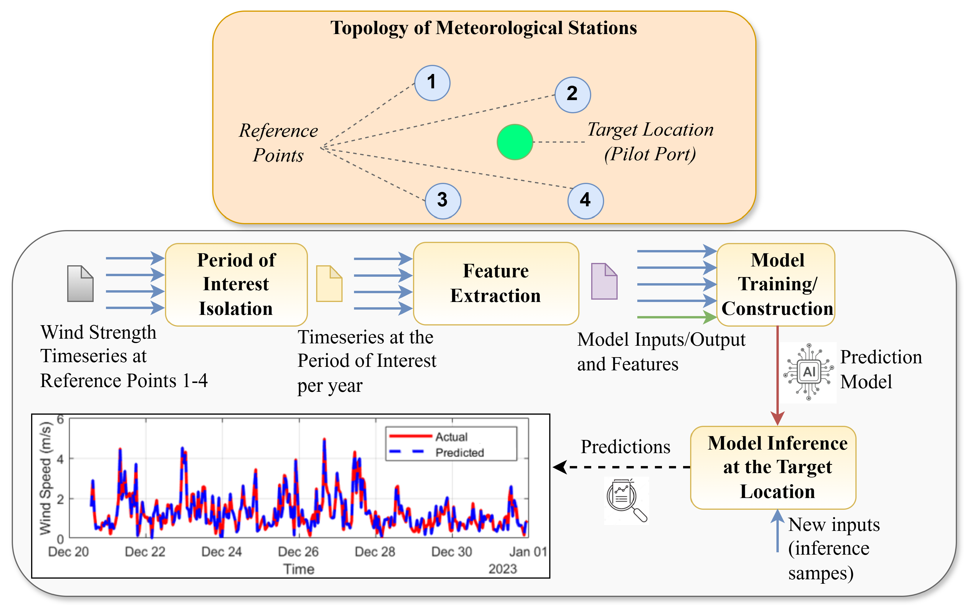
To enable wind strength estimation at coastal ports with limited direct meteorological data, we adopt a generic predictive framework that leverages neighboring reference points with historical records, as shown in Figure 8. The main idea is to exploit the spatiotemporal correlations between nearby ERA5 reanalysis stations and the data-scarce target location to train models that can reconstruct or predict wind behavior during desired time windows.
The proposed methodology, illustrated in Figure 8, consists of four primary stages. First, we perform Period of Interest Isolation, wherein we extract, from each year in the historical dataset, the wind strength time series that corresponds to the same day/month/hour as the available target measurements. The analysis is performed separately for the short-term and long-term periods of interest so as to test the proposed methodology in both short- and long-horizon predictions. This step ensures seasonally matched data across years and stations. Second, we conduct Feature Extraction by collecting the relevant wind speed values from the 4 reference locations, including also temporal lags as additional predictors, forming a structured feature matrix per timestamp. The third stage involves Model Construction, where deterministic or machine learning models are trained using the extracted input features from the reference points and the target wind speed values as desired outputs. The training is performed solely on real measurements at the target site and not synthetic data. Finally, in the Model Inference stage, the trained model is used to estimate wind strength at the target location using testing data not encountered during the training. This modular framework allows for consistent evaluation and fair comparison across multiple predictive strategies, as discussed in the subsequent subsections.

3.5. Wind Strength Prediction Models

This subsection presents the predictive models used to estimate the wind speed at the target port location using data from the four ERA5 reference points. Let v i ( t ) denote the wind speed at time t measured at reference location i, where i { 1 , 2 , 3 , 4 } . The goal of each model is to estimate v ^ ( t ) , the wind speed at the target location for the same timestamp t. While the term ‘prediction’ is commonly used in the machine learning literature to denote the model output, in this study, we refer specifically to the estimation of contemporaneous wind values at the target port using surrounding reference points.

3.5.1. Deterministic Models

Deterministic models predict the target wind speed using statistical, deterministic, or correlation-based relationships between the target and the reference locations, without requiring a learning phase [14]. Initially, deterministic models were constructed to predict wind speed at the target location. These models were based on both unweighted and weighted average techniques in order to find the accuracy of wind forecasting using simple models based on simple rules and statistical metrics (such as the average). The main advantage of these methods is their simplicity, since their creation and use exhibit low complexity and fast inference for forecasts generation. Furthermore, the use of such models for comparison purposes (baselines) with other more complex models (such as those of machine learning) can quantify the results of the latter compared to simple predictive techniques.
(1) Simple Averaging Model based on the last available year (SAM-last): The simplest approach assumes that the reference locations contribute equally to the wind dynamics at the target location, using the last year data. This model assumes that wind behavior at the target location is spatially homogeneous with respect to its neighboring reference points. That is, all reference points contribute equally to the wind field experienced at the target site, without requiring knowledge of their individual historical accuracy. In this version, the prediction is based exclusively on the most recent available year of ERA5 data (2023), which is assumed to best approximate the current wind regime. The predicted wind speed is computed as the arithmetic mean of the wind speeds at the four reference locations as:
v ^ SAM - last ( t ) = 1 4 i = 1 4 v i last ( t )
where v i last ( t ) is the wind speed at the i-th reference location at time t of the last year timeseries. Evidently, this model assumes that (i) all reference locations are equally informative, (ii) no spatial correlation filtering or weighting is applied, and (iii) recent historical patterns are more representative than previous long-term averages.
(2) Simple Averaging Model based on the significant-correlation years (SAM-sig): This model improves upon SAM-last by considering only the years that are statistically similar to the measurements at the target port, based on historical correlation. It acknowledges that not all historical years are equally representative and excludes those with weak or noisy relationships (Pearson’s Correlation Coefficient | r | < 0.3 ).
Let r j , target i be the Pearson’s correlation coefficient between the wind speeds at reference location i and year j and the target location across historical data. Define the set S i of significant years at reference location i as S i = { j [ 1970 , 2024 ] | r j , target i τ or r j , target i τ } , where τ is the correlation threshold (here 0.3). Then the predicted wind speed is:
v ^ SAM - sig ( t ) = 1 4 i = 1 4 1 | S i | j S i v i j ( t )
where v i j ( t ) is the wind speed at the i-th reference location at time t of the year j S i timeseries. Assumptions of this model include: (i) only years with | r | τ provide reliable estimates, and (ii) equal contribution from selected significant neighbors.
(3) Weighted Averaging Model based on the last available year (WAM-all): This model acknowledges that reference points influence the target location differently, based on their spatial and statistical similarity. Rather than applying a uniform average across reference points as in (4), it introduces a weighted average, where each reference location contributes proportionally to its correlation with the target. First, we define the correlation-derived weights as:
w i = r last , target i i = 1 4 r last , target i
where w i is the weight of reference point i, and r last , target i is the correlation coefficient between reference location i during the last year and the target location. Evidently, w i is computed as the ratio between the last-year correlation coefficient of reference point i and target location (numerator) and the sum (across reference locations) of all reference point-specific correlation coefficients. Then, the prediction is given by:
v ^ WAM - all ( t ) = i = 1 4 w i · v i last ( t )
As implied by (7), all four reference locations are retained and contribute to the model predictions, with their correlation strength determining their influence on the model. Also, the correlation structure is stationary over time.
(4) Weighted Averaging Model based on the significant-correlation years (WAM-sig): This model combines the selective filtering of SAM-sig in (5) with the proportional weighting of WAM-all. It discards weakly correlated locations and normalizes the correlation-based weights among the remaining significant ones. This approach prevents weakly relevant or noisy locations from distorting predictions. Hence, we firstly define the correlation-derived weights as:
w i = 1 | S i | j S i r j , target i i = 1 4 1 | S i | j S i r j , target i
where w i is the weight of reference point i, which is computed as the ratio between the mean (across significant-correlation years) correlation coefficient of reference point i and target location (numerator) and the sum (across reference locations) of all reference point-specific correlation coefficients. The prediction is finally given by:
v ^ WAM - sig ( t ) = i = 1 4 w i · 1 | S i | j S i v i j ( t )
Hence, in this model, only strongly correlated years or each location are used, while the weights reflect relative importance within selected year/location subset.

3.5.2. Machine Learning Models

Supervised machine learning models are designed to learn a mapping from predictor variables (features) to a target variable (response) based on historical observations [15,41]. In this study, we model the wind speed at the target location as a function of the wind speeds at the four reference ERA5 locations, including their past values over a lookback window of T time steps. Figure 9 shows the model structure for all ML models used in this work, while Figure 10 demonstrates the basic principles of the five ML models for supervised learning-based wind prediction.
Let the input feature vector at time t be defined as:
x ( t ) = [ v 1 ( t ) , v 1 ( t 1 ) , , v 1 ( t T ) , , v 4 ( t ) , v 4 ( t 1 ) , , v 4 ( t T ) ] T
where v i ( t ) is the wind speed at the reference point i and time t. The corresponding reconstructed target value is denoted as y ( t ) = v target ( t ) . The general ML model form is:
y ^ ( t ) = f ( x ( t ) ) + ϵ
where f ( · ) is the predictive function learned from the data, and ϵ is the residual error. Below, we provide a basic overview of the rationale and prediction formulation for each ML model.
(1) Multiple Linear Regression (MLR): MLR assumes a linear relationship between the inputs and the target variable [42]. It is interpretable and serves as a baseline model. The prediction formula can be written as:
y ^ MLR ( t ) = β 0 + i = 1 4 τ = 0 T β i , τ v i ( t τ )
where y ^ MLR ( t ) is MLR-predicted wind speed at the target location at time t, β 0 is the intercept term, β i , τ is the regression coefficient for the τ -lagged value from reference location i, v i ( t τ ) is the wind speed at reference location i at time t τ , and T is the lookback window size (number of past time steps). All the model parameters β are learned by solving the following least-squares minimization problem over N training samples::
β = arg min β t = 1 N ( y ( t ) y ^ MLR ( t ) ) 2
where β is the optimal model parameters. Evidently, during the training, this model fits a linear hyperplane (see Figure 10, MLR model) so that the mean squared error (computed over the training samples) between the actual and predicted values is minimized.
(2) Decision Tree Regression (DTR): DTR models learn hierarchical if-else rules to split the feature space into regions of similar target values [43]. They are non-parametric and can handle non-linear relationships between inputs and output. The input space is partitioned into J disjoint regions { R j } j = 1 J based on feature thresholds. The prediction at time t is:
y ^ DTR ( t ) = c j , if x ( t ) R j
where c j = 1 | R j | t : x ( t ) R j y ( t ) is the mean of the target values in region R j . Thus, the prediction at each leaf node outputs the average target value of samples in that region. The optimal tree is constructed by minimizing the total within-node variance:
{ R j } j = 1 J = arg min { R j } j = 1 J t : x ( t ) R j ( y ( t ) c j ) 2
Hence, a DTR model is a tree structure that, for any new input, the model finds the region (leaf node) it falls into (see Figure 10, DTR model). Finally, it returns the mean of the training target values in that region as the prediction.
(3) Support Vector Regression (SVR): SVR aims to find a function that approximates the target within a deviation ϵ , penalizing only large deviations and promoting flatness of the function [44]. Given a linear predictor f ( x ) = w T x + b , the primal form of the optimization problem is:
min w , b , ξ , ξ 1 2 w 2 + C t = 1 N ( ξ t + ξ t )
subject to:
y ( t ) w T x ( t ) b ϵ + ξ t w T x ( t ) + b y ( t ) ϵ + ξ t ξ t , ξ t 0
where w R 4 ( T + 1 ) is the weight vector, b R is a bias term, ϵ > 0 is the insensitive error margin, ξ t , ξ t 0 are slack variables for margin violations, and C > 0 is the regularization parameter balancing flatness and errors. For non-linear patterns, SVR uses a kernel function to map inputs to a high-dimensional space.
(4) Random Forest Regression (RFR): RFR builds an ensemble of B decision trees, each trained on a bootstrap sample of the data (with T lags included), with random feature selection, and aggregates their predictions to reduce variance [45]. Therefore, it reduces overfitting and increases robustness. Let T b ( t ) denote the prediction of the b-th tree using lag-augmented features. The ensemble prediction is:
y ^ RFR ( t ) = 1 B b = 1 B T b ( x ( t ) )
Each tree b is trained to minimize the squared error in its regions, as defined in (15). Thus, the forest aggregates individual tree prediction to make the final prediction.
(5) Gradient Boosting Regression (GBR): GBR trains additive decision trees sequentially, each one correcting the residuals of the previous ensemble to iteratively reduce the prediction error [46]. It often yields superior accuracy in structured data. Starting with an initial prediction y ^ GBR ( 0 ) ( t ) (e.g., mean of y), at each training stage m, a new tree h m ( t ) is fit to the residuals:
y ^ GBR ( 0 ) ( t ) = y ¯ , y ^ GBR ( m ) ( t ) = y ^ GBR ( m 1 ) ( t ) + η h m ( x ( t ) ) , m = 1 , , M
where η is the learning rate controlling the contribution of each tree, M is the number of boosting iterations, h m is the regression tree fitted to residuals of stage m 1 , and y ¯ is the mean of training target values. The final GBR prediction is:
y ^ GBR ( t ) = m = 1 M η h m ( x ( t ) )
Regarding the objective function in GBR training, at each stage m, the tree h m is trained to minimize the loss:
min h m t = 1 N y ( t ) y ^ GBR ( m 1 ) ( t ) h m ( x ( t ) ) 2
Each iteration improves upon the current model by approximating the negative gradient of the loss function. Each of these models is evaluated under identical input-output data for fair comparison, incorporating both current and lagged wind observations from the reference points.

4. Numerical Results and Performance Evaluation

In this section, we present the experimental setup and the performance evaluation of the wind prediction models, as analytically presented in Section 3. The results are based on real measurements of meteorological stations deployed at the reference points and the Greek pilot port (Chalkida).

4.1. Experimental Setup

To evaluate the performance of the proposed wind strength prediction methodology, we define the Chalkida port as the target location. The main objective is to predict the wind speed at this location based on historical measurements from four surrounding reference points derived from the ERA5 reanalysis dataset. Two prediction periods are considered, including the short-term window (20–31 December 2023) and the long-term window (26 February–29 October 2024). The two prediction windows were selected based on the availability and operational status of the pilot wind measurement station installed at the Chalkida port. Specifically, the short-term window (20–31 December 2023) corresponds to a densely sampled period shortly after deployment, while the long-term window (26 February–29 October 2024) represents a wider seasonal horizon during which the station maintained reliable operation. These periods were chosen to enable evaluation of both short-term fitting accuracy and long-term generalization under diverse weather conditions.
For each prediction instance, the input features consist of the wind speed values (computed from the u 10 and v 10 components) at the four reference points, along with their two temporal lags. The prediction task is modeled as a supervised regression problem. Each learning algorithm is trained using time-aligned samples from the 54-year ERA5 archive, considering seasonally matched instances (same day-of-year and hour).
The primary evaluation metric is the Mean Squared Error (MSE), computed between the predicted and actual wind speed values. In addition to numerical scores, we also perform a visual inspection by plotting the actual vs. predicted values for each model, facilitating a qualitative comparison of tracking accuracy, peak estimation, and error bursts.

4.2. Prediction Curves and Fitting Performance

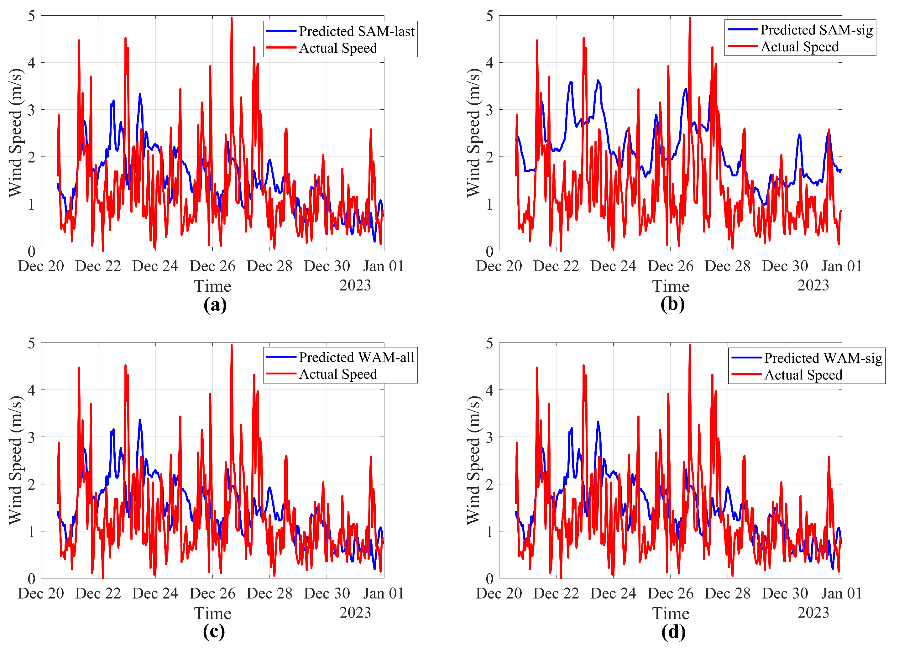
To qualitatively assess the temporal alignment between predicted and actual wind speed values, we analyze the short-term prediction performance across all evaluated models for the period 20–31 December 2023. This window allows for high-resolution inspection of the fitting capability of each model on real measurements at the Chalkida port. Figure 11 illustrates the performance of the four deterministic schemes, presenting the time-series plots comparing the predicted wind speed to the actual observed values for each of the nine models. The deterministic models (SAM-last, SAM-sig, WAM-all, WAM-sig) demonstrate limited capability in capturing the dynamic range and transient fluctuations of wind speed. Specifically, the SAM-last and SAM-sig variants tend to underestimate peaks and delay abrupt changes, reflecting their reliance on historical averages without real-time adaptivity. The weighted averaging variants (WAM-all and WAM-sig) show slightly better alignment, particularly during periods of moderate wind, due to the incorporation of correlation-informed weights. However, they still fail to reconstruct high-frequency variations. This is due to the lack of adaptiveness in deterministic schemes, which treat each forecasted hour independently of temporal dynamics.
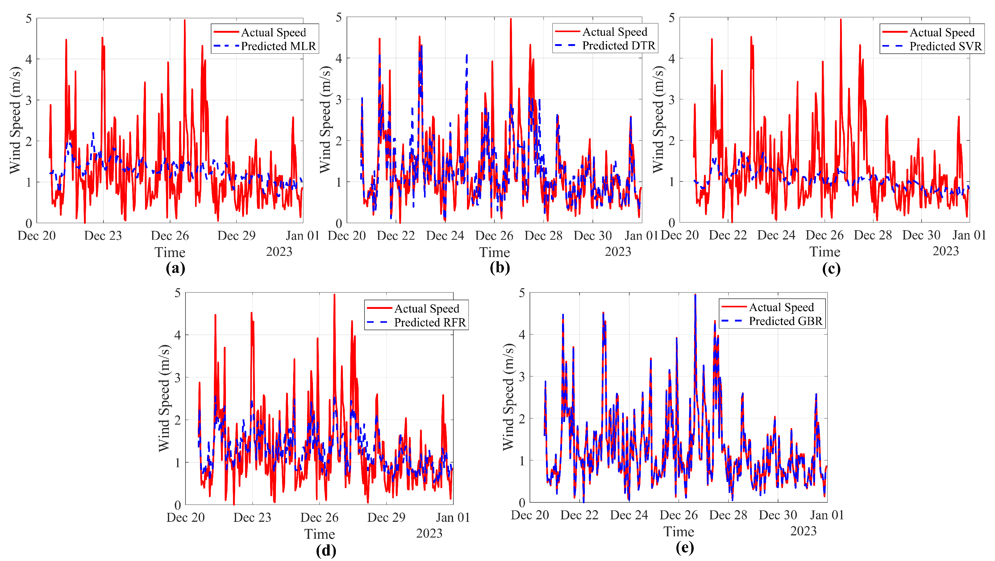
In contrast, Figure 12 demonstrates the performance of ML models. The ML models exhibit substantially improved fitting behavior, with predictions closely following the trajectory of the ground truth. Among them, the GBR achieves the most accurate curve reconstruction, capturing both the amplitude and timing of peaks, while also minimizing deviation in lower wind regions. The DTR also shows strong agreement, especially in low and mid-range speeds, although it occasionally introduces step-wise artifacts due to its piecewise constant structure. On the other hand, the RFR provides smooth and relatively accurate forecasts, though slightly less responsive to sharp transitions. The SVR underperforms in this context, showing limited flexibility in peak tracking, which may be attributed to poor kernel generalization. The MLR model yields consistently biased estimates, confirming its inability to capture the nonlinear spatiotemporal dependencies underlying the wind patterns. Overall, this visual analysis reinforces the superiority of ensemble-based and tree-based models, particularly GBR, in reconstructing complex wind dynamics from neighboring station data. These results underscore the importance of model expressiveness when addressing wind pattern reconstruction in data-scarce coastal regions, where high temporal accuracy is crucial for operational planning and safety.

4.3. Comparative Performance Between Different Models

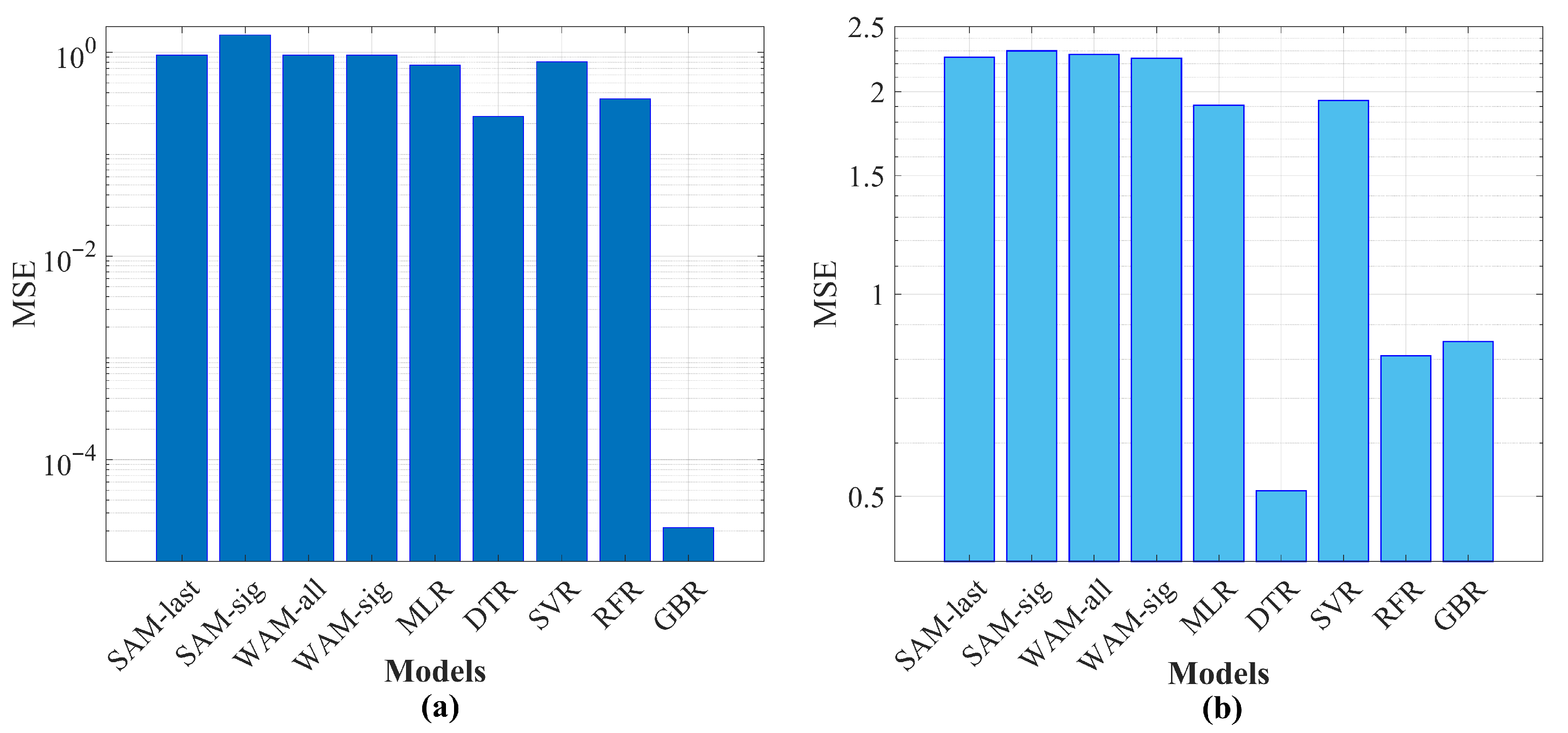
To systematically evaluate the forecasting capabilities of the examined models, we compute and compare the Mean Squared Error (MSE) across both short-term (11-day) and long-term (8-month) prediction horizons. The results, summarized in Figure 13, reveal critical differences in performance trends depending on the model class and the temporal scale of prediction.
In the short-term analysis shown in Figure 13a, deterministic models such as SAM-last, SAM-sig, WAM-all, and WAM-sig consistently exhibit higher MSE values ( MSE 1 ), highlighting their inability to track fine-grained and rapid changes in wind speed. This is expected given their averaging-based static nature, which smooths over temporal dynamics and leads to loss of detail. MLR achieves slightly improved accuracy, but fails to capture nonlinear dependencies. Among machine learning models, GBR clearly outperforms all others, achieving the lowest MSE by a significant margin (below 10 4 ), followed by RFR and DTR. These results underscore the importance of ensemble learning and nonlinearity modeling for high-resolution short-term wind forecasting.
In the long-term prediction scenario depicted in Figure 13b, all models experience an increase in MSE, reflecting the accumulated uncertainty over extended periods. Deterministic and linear models maintain poor performance ( MSE 2.2 ), whereas machine learning models, especially DTR, RFR and GBR, demonstrate superior long-horizon generalization. Notably, DTR marginally outperforms GBR and RFR in this setting, indicating its robustness and ability to approximate nonlinear patterns using simple tree partitions with limited overfitting. These findings suggest that the optimal wind speed prediction model is horizon-dependent, indicating that ensemble models like GBR excel in short-term accuracy due to their bias-reducing additive architecture, while simpler tree-based models such as DTR offer more stable generalization across months. This highlights the necessity of adapting model selection to the intended temporal resolution of the application.
It is noteworthy that the GBR model achieves an extremely low MSE (< 10 4 ) in the short-horizon window. This outcome is attributable to strong temporal consistency during the 11-day period and the ability of GBR’s sequential boosting mechanism to iteratively correct residual errors. While other short-term windows may yield higher absolute errors depending on meteorological variability, GBR is still expected to outperform the other models in most short-horizon scenarios. In contrast, the long-horizon evaluation exhibits larger and more realistic error levels due to greater temporal variability, highlighting how model performance depends on the forecasting context.
Is it worth noting that, while the optimal predictor may vary depending on the dataset characteristics and forecasting horizon, the proposed methodology is general-purpose and agnostic to the underlying model, allowing for periodic retraining and iterative selection of the most appropriate model based on updated input-output data. This adaptability ensures robust and dynamic prediction pipelines suitable for real-world deployment and up-to-date wind strength forecasts.

4.4. Multi-Metric Performance Evaluation

To ensure a rigorous and comprehensive assessment of model performance, we extend our evaluation beyond the commonly used MSE and employ a suite of complementary error metrics. While MSE quantifies the average squared deviation between predicted and observed wind speed values, it is sensitive to outliers and does not capture all dimensions of predictive quality. For wind speed estimation in coastal environments, where both absolute accuracy and structural fidelity of temporal dynamics are important, a broader set of metrics is necessary. Considering the short-term window, we incorporate additional measures that evaluate absolute error magnitude, proportional bias, explained variance, agreement in variability, and similarity in spectral characteristics.
Let y = [ y 1 , y 2 , , y N ] denote the actual wind speed time series and y ^ = [ y ^ 1 , y ^ 2 , , y ^ N ] the corresponding predicted values, where N is the number of samples. The Mean Absolute Error (MAE) is defined as:
MAE = 1 N i = 1 N | y i y ^ i | ,
and expresses the average magnitude of absolute prediction errors in units of m/s. Unlike MSE, it weights all deviations linearly. The Root Mean Squared Error (RMSE) is given by:
RMSE = 1 N i = 1 N ( y i y ^ i ) 2 ,
providing an error metric that penalizes larger deviations more strongly and retains the same physical units as the wind speed measurements. The Mean Absolute Percentage Error (MAPE) is calculated as:
MAPE = 100 % N i = 1 N y i y ^ i y i + ϵ ,
where ϵ is a small constant introduced to avoid division by zero (here set at 0.0001 ). MAPE expresses the average error as a percentage of the observed signal and is useful when comparing performance across different magnitudes, although it can become unstable for very low wind speeds. The Coefficient of Determination ( R 2 ) is defined as:
R 2 = 1 i = 1 N ( y i y ^ i ) 2 i = 1 N ( y i y ¯ ) 2 ,
where y ¯ = 1 N i = 1 N y i is the sample mean. This metric quantifies the proportion of variance in the observed data that is explained by the model, with values closer to 1 indicating stronger explanatory power ( R 2 can also be negative for poor model performance). Willmott’s Index of Agreement d, which measures the degree of model-data correspondence, is expressed as:
d = 1 i = 1 N ( y i y ^ i ) 2 i = 1 N | y ^ i y ¯ | + | y i y ¯ | 2 .
The index ranges from 0 (no agreement) to 1 (perfect agreement) and is particularly sensitive to bias and scale differences between model output and observations. To assess the fidelity of predicted wind speed signals in the frequency domain, we additionally compute a Spectral Fitness Score (SFS). Let F ( y ) and F ( y ^ ) denote the discrete Fourier transforms (DFT) of the observed and predicted signals, respectively. The SFS is defined as:
SFS = 1 | F ( y ) | | F ( y ^ ) | 2 | F ( y ) | 2 ,
where | F ( · ) | denotes the magnitude spectrum (after Fourier transformation) and · 2 is the Euclidean norm. This metric reflects the goodness of fit between the predicted ans actual spectra, and evaluates how well each model preserves the underlying temporal frequency structure. Table 2 summarizes the evaluation metrics per model.
Evidently from Table 2, the GBR model clearly outperforms all others, achieving the lowest errors (MSE, MAE, RMSE, MAPE) and the highest agreement metrics ( R 2 , WI, and SFS), indicating excessive accuracy as well as strong preservation of temporal and spectral wind speed structure. Ensemble methods such as DTR and RFR also show competitive performance, whereas all deterministic baselines exhibit substantially higher errors and negative or near-zero R 2 values, reflecting their inability to represent nonlinear or rapidly varying wind behavior. The spectral analysis further confirms that GBR more accurately reconstructs the oscillatory patterns present in the real wind signal.
To further investigate model robustness under different wind conditions, MSE, MAPE, RMSE, and MAPE metrics were also computed across discrete wind speed ranges derived from Beaufort-scale thresholds. To ensure enough samples per wind range, wind intervals were selected for calm/light breeze conditions (0–3.3 m/s) and gentle/strong breeze conditions (greater than 3.3 m/s). Evaluating each model within these ranges provides insight into their behavior under operationally significant scenarios, since accuracy during calm or strong winds is particularly important for port safety and maritime situational awareness. Table 2 summarizes the evaluation metrics per model for each wind speed category.
Table 3 presents a breakdown of model performance across two wind speed ranges, namely low (≤ 3.3 m/s) and high (> 3.3 m/s). The results show that all models perform significantly better in the low-wind regime, with consistently lower errors (MSE, MAE, RMSE, MAPE). Among them, the GBR model maintains outstanding accuracy in both regimes, exhibiting minimal degradation under higher wind speeds. In contrast, deterministic models (SAM/WAM) show considerable estimation errors under high wind conditions, suggesting limited adaptability to more variable or extreme wind patterns. Machine learning models, particularly GBR (and secondly DTR), demonstrate superior robustness across regimes, validating their suitability for capturing both calm and stronger wind dynamics at port locations.

4.5. Time Lag Effect and Feature Importance

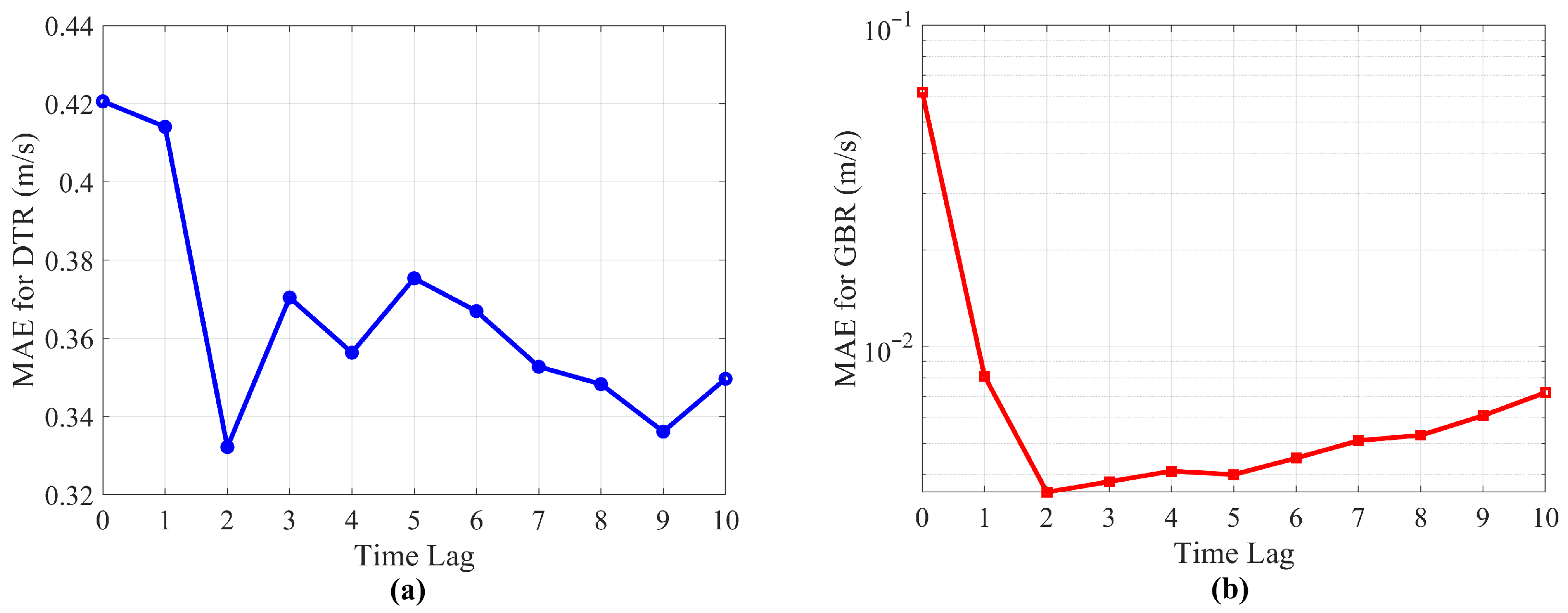
In this section, we aim to better interpret the model behavior and assess the contribution of input features by evaluating (i) how prediction accuracy is affected by the inclusion of past observations (time-lagged terms), and (ii) which reference points and lag values contribute most to accurate predictions. To analyze the impact of temporal memory, we evaluated the MAE of the highest-accuracy models observed in the previous analyses, namely the DTR and GBR models, under varying time lag values. For each experiment, only a single lag level was used across the four reference points. That is, for time lag T { 0 , 1 , , 10 } , the input to each model was the set of four reference wind speed values observed at lag T prior to the current time. Figure 14 illustrates the MAE versus lag index. For DTR, the MAE gradually decreases as more past information is incorporated, showing the minimum MAE at T = 2 steps. In addition, the GBR model shows a very sharp decrease in error for lags 0 to 2, reaching the minimum MAE for T = 2 steps. Note that, for lags greater than 2, GBR MAE slightly increases due to increased model complexity (more inputs are considered). This confirms that the optimal model performance is observed for T = 2 , ensuring a balanced trade-off between estimation performance and complexity.
To further justify the model’s internal logic, we performed a feature importance analysis using the trained DTR and GBR models with a fixed time lag of 2 (as the optimal configuration). This configuration corresponds to twelve input features, since each of the four reference points provides three lagged values (lags 0, 1, and 2). The importance of each feature was computed based on a permutation-based approach [47]. Specifically, for each input feature, its values were randomly shuffled across all data samples while keeping all other features unchanged. The change in model performance, measured via the increase in prediction error (specifically, Mean Squared Error), was then recorded [47]. Features that cause a higher degradation in performance when perturbed are considered more important. This method captures both the direct predictive value of each feature and its interactions with others, offering an interpretable view of the model’s decision process. The resulting importance scores for each feature are illustrated in Figure 15.
Evidently from Figure 15, both models attribute the highest importance to the most recent (lag 0) value of Reference Point 1, which is closest to the target location. GBR assigns more balanced contributions across all four reference points, whereas DTR assigns relatively more importance to Reference Points 1 and 3. This aligns with the physical intuition that nearby offshore points (closer to Chalkida) exert a stronger influence, with all reference points and their lags contributing to the wind speed estimation at the target port.

5. Discussion

The comparative evaluation of the proposed wind prediction models highlights distinct strengths and limitations between deterministic and machine learning approaches. Deterministic models, while simple, fast and computationally efficient, rely on fixed statistical aggregation (e.g., means, correlations) and thus lack the capacity to capture nonlinear or time-varying dependencies in the data. Their performance deteriorates in scenarios involving rapidly fluctuating or spatially diverse wind fields. In contrast, machine learning models, particularly ensemble-based regressors like Gradient Boosting, exhibit superior adaptability to the complex, nonlinear, and multiscale dependencies observed in coastal wind patterns. These models are capable of learning intricate spatiotemporal mappings between reference stations and the target port. Notably, the best-performing model shifts depending on the prediction horizon (short-term vs. long-term) and data characteristics, emphasizing the need for a dynamic model selection strategy embedded in a continuously updated learning framework.
The comparative evaluation of predictive models reveals important insights into their underlying mechanisms and suitability for wind estimation. Deterministic models, such as simple or weighted averaging schemes (SAM and WAM), offer low computational complexity and interpretability but lack the flexibility to capture complex and non-linear dependencies in the data. Ensemble learning methods, particularly GBR (and RFR only for the long-term period), consistently demonstrated superior performance, attributed to their robustness against overfitting and their ability to capture complex, non-linear interactions among spatially distributed inputs. These methods effectively exploit the spatiotemporal structure of the historical data, learning repeated seasonal patterns and spatial dependencies across reference locations. On the other hand, MLR, being a linear estimator, struggled with the non-linear nature of wind behavior, resulting in systematically higher errors. DTR, though capable of capturing non-linearity, was prone to overfitting and variance in the short-horizon evaluation window. SVR provided moderate performance, suggesting that while kernel-based methods are promising, their performance is sensitive to parameter tuning and data scaling. It is noteworthy that simpler models such as MLR and SVR showed limited predictive accuracy across both short- and long-term horizons. This can be attributed to their inability to fully capture the nonlinear and multi-dimensional dynamics of wind behavior in coastal environments. MLR assumes linear dependencies, which oversimplifies the underlying atmospheric processes. On the other hand, SVR, although nonlinear through kernel mapping, is sensitive to the choice of hyperparameters and may not effectively learn from partially correlated and temporally lagged inputs. Overall, these findings highlight the importance of model flexibility and the need for richer representations when modeling meteorological data.
From a practical standpoint, the proposed data-driven framework offers a scalable and low-cost solution for wind monitoring in under-instrumented ports, effectively enabling virtual wind stations based on data from surrounding reference points and historical records. Such virtual sensors can support operational decision-making, early warning systems, and resilience planning in ports with limited meteorological infrastructure. However, several challenges must be addressed for robust deployment. First, wind patterns exhibit non-stationary behavior due to climate dynamics and land-sea interactions, which may limit long-term model stability. Second, model accuracy is sensitive to temporal alignment, seasonal matching, and preprocessing procedures (e.g., lag selection, feature engineering), requiring careful pipeline design. Addressing these challenges calls for the integration of adaptive learning, domain-specific knowledge, and real-time data assimilation in future research and applications.
While our methodology leverages 54 years of historical ERA5 data to model and reconstruct wind speeds at the target location, we acknowledge that climate anomalies or non-stationary behavior (e.g., extreme years or gradual trends due to climate change) may introduce bias in the learned relationships. The inclusion of such years in the training dataset without consideration of their atypical behavior may affect model generalization in unseen or shifting conditions. Future research could incorporate anomaly detection techniques or climate similarity filtering to weight historical years based on their meteorological proximity to the target period. Additionally, incorporating global or regional climate indices as exogenous variables may further improve robustness against interannual variability.

Limitations

Despite the presented advantages and performance of the proposed estimation framework, several methodological limitations should be acknowledged. First, the approach is constrained by the spatial resolution and representativeness of the ERA5 reanalysis dataset, which may not capture fine-scale variations in ports with complex topography. Second, the feature set used in training, primarily wind speed values and their lags, is relatively narrow and does not include potentially informative variables such as temperature, pressure, humidity, or orographic effects. Third, the study’s validation is limited to a single port, requiring generalizability to ports with more variable wind regimes. Furthermore, the use of multi-decade data carries the risk of including climatologically atypical years, which may distort the training process if not explicitly addressed. Finally, the framework currently lacks an online learning component, limiting its ability to adapt to shifts in weather patterns or sensor drift over time. These limitations highlight avenues for methodological refinement and expansion in future work.
A key limitation of the current study is the exclusive focus on a single coastal port (Chalkida), characterized by relatively stable wind directions and moderate topographic complexity. While this supports model fitting, it limits conclusions about broader generalization. Nevertheless, the proposed framework is inherently general-purpose and can be applied to construct multiple virtual wind stations by repeating the methodology across different geographic grids, each defined by a set of reference points and one or more internal targets. Future work can focus on deploying the approach across diverse coastal environments (e.g., in the Aegean and Mediterranean), including ports with more extreme climate variability and topographically complex shorelines, to validate robustness and adaptability.

6. Conclusions and Future Work

This study introduced a spatiotemporal framework for wind speed estimation in ports with limited on-site measurements, using surrogate data from neighboring meteorological stations and long-term historical archives. We systematically evaluated a suite of models, including both deterministic predictors based on statistical aggregation and supervised machine learning algorithms trained across decades of hourly data. The framework was validated using real-world measurements from the Chalkida pilot port over two distinct periods (short- and long-horizon), revealing that the best-performing model varies depending on the temporal context and data richness. Ensemble learning methods, particularly Gradient Boosting Regressors, demonstrated superior accuracy in short-term forecasting, while tree-based regressors remained competitive over extended prediction windows.
Future extensions of this work will aim to enhance prediction fidelity and robustness by integrating additional physical and geographical features, such as topographical elevation, sea–land thermal gradients, and surface temperature data, to better capture environmental heterogeneity [48]. While the proposed framework demonstrates strong predictive capability using only wind speed information from four reference points and limited lagged terms, coastal wind fields are strongly influenced by diurnal sea–land breeze effects driven by thermal contrasts. Future extensions of this work can incorporate additional exogenous meteorological features, such as temperature gradients, pressure fields, and sea-surface thermodynamic variables, as well as explicit diurnal cycle descriptors, which are expected to further improve the model’s ability to represent mesoscale coastal dynamics. Moreover, the framework can be extended toward real-time wind forecasting by incorporating exogenous weather predictions [49]. While this study was conducted using ERA5 reanalysis data, the proposed methodology is dataset-agnostic and can be extended to other sources, including satellite-based products such as ASCAT. Future work can explore how satellite data can complement reanalysis inputs in multi-source machine learning frameworks for virtual wind station deployment. Future work can also focus on targeted analysis of model performance during high wind events. This includes defining wind intensity thresholds, analyzing conditional biases in extreme conditions, and incorporating specialized methods such as quantile regressors or oversampling techniques to better capture rare but operationally critical wind fluctuations. Finally, the methodology can be scaled to a multi-port setup, enabling virtual monitoring stations across several key ports in the Aegean and Mediterranean areas, thus supporting broader maritime situational awareness and planning.

Author Contributions

Conceptualization, A.G. and A.K.; methodology, A.G.; software, A.G.; validation, A.K., M.H. and P.T.; formal analysis, A.G.; investigation, A.K., M.H. and P.T.; resources, A.K. and M.H.; data curation, A.K.; writing—original draft preparation, A.G. and A.K.; writing—review and editing, M.H. and P.T.; visualization, A.G.; supervision, A.K. and M.H.; project administration, A.K. and M.H.; funding acquisition, A.K. All authors have read and agreed to the published version of the manuscript.

Funding

This research received no external funding.

Data Availability Statement

The data presented in this study are available on request from the authors due to privacy restrictions.

Acknowledgments

The authors acknowledge that the work has been carried out in part by the research project “AdaptPorts—Ports Climate Mitigation and Adaptation Strategy” funded by the Green Fund of Greece, Priority Axis 3 “RESEARCH AND APPLICATION”, “PHYSICAL ENVIRONMENT & INNOVATIVE ACTIONS 2022”.

Conflicts of Interest

The authors declare no conflicts of interest.

Abbreviations

The following abbreviations are used in this manuscript:
ECMWF European Centre for Medium-Range Weather Forecasts
MLR Multivariate Linear Regression
DTR Decision Tree Regression
SVR Support Vector Regression
RFR Random Forest Regression
GBR Gradient Boosting Regression
IDW Inverse Distance Weighting
GBM Gradient Boost Machine
ML Machine Learning
DL Deep Learning
AIArtificial Intelligence
MSEMean Squared Error
ANNArtificial Neural Network
SVMSupport Vector Machine
CNNConvolutional Neural Network
LSTMLong Short Term Memory
HTMLHypertext Markup Language
SAM-lastSimple Averaging Model based on the last available year
SAM-sigSimple Averaging Model based on the significant-correlation years
WAM-allWeighted Averaging Model based on the last available year
WAM-sigWeighted Averaging Model based on the significant-correlation years

References

  1. Balas, E.A.; Balas, C.E. Maritime Risk Assessment: A Cutting-Edge Hybrid Model Integrating Automated Machine Learning and Deep Learning with Hydrodynamic and Monte Carlo Simulations. J. Mar. Sci. Eng. 2025, 13, 939. [Google Scholar] [CrossRef]
  2. Giannopoulos, A.; Gkonis, P.; Kalafatelis, A.; Nomikos, N.; Spantideas, S.; Trakadas, P.; Syriopoulos, T. From 6G to SeaX-G: Integrated 6G TN/NTN for AI-Assisted Maritime Communications—Architecture, Enablers, and Optimization Problems. J. Mar. Sci. Eng. 2025, 13, 1103. [Google Scholar] [CrossRef]
  3. Puig, M.; Cirera, A.; Wooldridge, C.; Sakellariadou, F.; Darbra, R.M. Mega Ports’ mitigation response and adaptation to climate change. J. Mar. Sci. Eng. 2024, 12, 1112. [Google Scholar] [CrossRef]
  4. Monioudi, I.N.; Chatzistratis, D.; Moschopoulos, K.; Velegrakis, A.F.; Polydoropoulou, A.; Chalazas, T.; Bouhouras, E.; Papaioannou, G.; Karakikes, I.; Thanopoulou, H. Exposure of Greek Ports to Marine Flooding and Extreme Heat Under Climate Change: An Assessment. Water 2025, 17, 1897. [Google Scholar] [CrossRef]
  5. Verschuur, J.; Koks, E.E.; Hall, J.W. Systemic risks from climate-related disruptions at ports. Nat. Clim. Change 2023, 13, 804–806. [Google Scholar] [CrossRef]
  6. Sáenz, S.S.; Diaz-Hernandez, G.; Schweter, L.; Nordbeck, P. Analysis of the mooring effects of future ultra-large container vessels (ULCV) on port infrastructures. J. Mar. Sci. Eng. 2023, 11, 856. [Google Scholar] [CrossRef]
  7. Gottschall, J.; Dörenkämper, M. Understanding and mitigating the impact of data gaps on offshore wind resource estimates. Wind. Energy Sci. Discuss. 2020, 2020, 1–22. [Google Scholar] [CrossRef]
  8. Gutiérrez, C.; Molina, M.; Ortega, M.; Lopez-Franca, N.; Sánchez, E. Low-wind climatology (1979–2018) over Europe from ERA5 reanalysis. Clim. Dyn. 2024, 62, 4155–4170. [Google Scholar] [CrossRef]
  9. Alkhalidi, M.; Al-Dabbous, A.; Al-Dabbous, S.; Alzaid, D. Evaluating the accuracy of the ERA5 model in predicting wind speeds across coastal and offshore regions. J. Mar. Sci. Eng. 2025, 13, 149. [Google Scholar] [CrossRef]
  10. Hallgren, C.; Aird, J.A.; Ivanell, S.; Körnich, H.; Vakkari, V.; Barthelmie, R.J.; Pryor, S.C.; Sahlée, E. Machine learning methods to improve spatial predictions of coastal wind speed profiles and low-level jets using single-level ERA5 data. Wind. Energy Sci. Discuss. 2023, 2023, 1–30. [Google Scholar] [CrossRef]
  11. Zambra, M.; Farrugia, N.; Cazau, D.; Gensse, A.; Fablet, R. Multimodal learning–based reconstruction of high-resolution spatial wind speed fields. Environ. Data Sci. 2025, 4, e2. [Google Scholar] [CrossRef]
  12. Baki, H.; Basu, S. Estimating high-resolution profiles of wind speeds from a global reanalysis dataset using TabNet. Environ. Data Sci. 2024, 3, e32. [Google Scholar] [CrossRef]
  13. Skianis, K.; Giannopoulos, A.; Spantideas, S.; Hatzaki, M.; Karditsa, A.; Trakadas, P. SWIRL: Statistical downscaling for Wind Pattern Reconstruction using Machine Learning. In Proceedings of the 18th International Conference on Environmental Science and Technology (CEST), Athens, Greece, 30 August–2 September 2023. [Google Scholar]
  14. Cavaiola, M.; Tuju, P.E.; Mazzino, A. Accurate and efficient AI-assisted paradigm for adding granularity to ERA5 precipitation reanalysis. Sci. Rep. 2024, 14, 26158. [Google Scholar] [CrossRef] [PubMed]
  15. Khattak, A.; Chan, P.W.; Chen, F.; Peng, H. Time-series prediction of intense wind shear using machine learning algorithms: A case study of Hong Kong International Airport. Atmosphere 2023, 14, 268. [Google Scholar] [CrossRef]
  16. Ratnam, J.; Behera, S.K.; Nonaka, M.; Martineau, P.; Patil, K.R. Predicting maximum temperatures over India 10-days ahead using machine learning models. Sci. Rep. 2023, 13, 17208. [Google Scholar] [CrossRef]
  17. Giannopoulos, A.E.; Spantideas, S.T.; Zetas, M.; Nomikos, N.; Trakadas, P. Fedship: Federated over-the-air learning for communication-efficient and privacy-aware smart shipping in 6g communications. IEEE Trans. Intell. Transp. Syst. 2024, 25, 19873–19888. [Google Scholar] [CrossRef]
  18. Dupuy, F.; Durand, P.; Hedde, T. Downscaling of surface wind forecasts using convolutional neural networks. Nonlinear Process. Geophys. 2023, 30, 553–570. [Google Scholar] [CrossRef]
  19. Lussana, C.; Salvati, M.; Pellegrini, U.; Uboldi, F. Efficient high-resolution 3-D interpolation of meteorological variables for operational use. Adv. Sci. Res. 2009, 3, 105–112. [Google Scholar] [CrossRef]
  20. Ryu, S.; Song, J.J.; Lee, G. Interpolation of temperature in a mountainous region using heterogeneous observation networks. Atmosphere 2024, 15, 1018. [Google Scholar] [CrossRef]
  21. Winstral, A.; Jonas, T.; Helbig, N. Statistical downscaling of gridded wind speed data using local topography. J. Hydrometeorol. 2017, 18, 335–348. [Google Scholar] [CrossRef]
  22. Talbot, C.; Bou-Zeid, E.; Smith, J. Nested mesoscale large-eddy simulations with WRF: Performance in real test cases. J. Hydrometeorol. 2012, 13, 1421–1441. [Google Scholar] [CrossRef]
  23. Slater, L.J.; Arnal, L.; Boucher, M.A.; Chang, A.Y.Y.; Moulds, S.; Murphy, C.; Nearing, G.; Shalev, G.; Shen, C.; Speight, L.; et al. Hybrid forecasting: Blending climate predictions with AI models. Hydrol. Earth Syst. Sci. 2023, 27, 1865–1889. [Google Scholar] [CrossRef]
  24. Yadav, K.; Malviya, S.; Tiwari, A.K. Improving Weather Forecasting in Remote Regions Through Machine Learning. Atmosphere 2025, 16, 587. [Google Scholar] [CrossRef]
  25. Leme Beu, C.M.; Landulfo, E. Machine-learning-based estimate of the wind speed over complex terrain using the long short-term memory (LSTM) recurrent neural network. Wind Energy Sci. 2024, 9, 1431–1450. [Google Scholar] [CrossRef]
  26. Schulz, B.; Lerch, S. Machine learning methods for postprocessing ensemble forecasts of wind gusts: A systematic comparison. Mon. Weather. Rev. 2022, 150, 235–257. [Google Scholar] [CrossRef]
  27. Zetas, M.; Spantideas, S.; Giannopoulos, A.; Nomikos, N.; Trakadas, P. Empowering 6G maritime communications with distributed intelligence and over-the-air model sharing. Front. Commun. Netw. 2024, 4, 1280602. [Google Scholar] [CrossRef]
  28. Alkhayat, G.; Mehmood, R. A review and taxonomy of wind and solar energy forecasting methods based on deep learning. Energy AI 2021, 4, 100060. [Google Scholar] [CrossRef]
  29. Sun, F.; Hao, W.; Zou, A.; Shen, Q. A survey on spatio-temporal series prediction with deep learning: Taxonomy, applications, and future directions. Neural Comput. Appl. 2024, 36, 9919–9943. [Google Scholar] [CrossRef]
  30. Zhao, Y.; Du, X.; Li, Q.; Zhang, Y.; Wang, H.; Wang, Y.; Xu, J.; Xiao, J.; Shen, Y.; Dong, Y.; et al. Mapping and Analyzing Winter Wheat Yields in the Huang-Huai-Hai Plain: A Climate-Independent Perspective. Remote Sens. 2025, 17, 1409. [Google Scholar] [CrossRef]
  31. Baïle, R.; Muzy, J.F. Leveraging data from nearby stations to improve short-term wind speed forecasts. Energy 2023, 263, 125644. [Google Scholar] [CrossRef]
  32. Shestakova, A.A.; Fedotova, E.V.; Lyulyukin, V.S. Relevance of Era5 reanalysis for wind energy applications: Comparison with sodar observations. Geogr. Environ. Sustain. 2024, 17, 54–66. [Google Scholar] [CrossRef]
  33. Hersbach, H.; Bell, B.; Berrisford, P.; Hirahara, S.; Horányi, A.; Muñoz-Sabater, J.; Nicolas, J.; Peubey, C.; Radu, R.; Schepers, D.; et al. The ERA5 global reanalysis. Q. J. R. Meteorol. Soc. 2020, 146, 1999–2049. [Google Scholar] [CrossRef]
  34. Cucchi, M.; Weedon, G.P.; Amici, A.; Bellouin, N.; Lange, S.; Schmied, H.M.; Hersbach, H.; Buontempo, C. WFDE5: Bias adjusted ERA5 reanalysis data for impact studies. Earth Syst. Sci. Data 2020, 12, 2097–2120. [Google Scholar] [CrossRef]
  35. Hassler, B.; Lauer, A. Comparison of reanalysis and observational precipitation datasets including ERA5 and WFDE5. Atmosphere 2021, 12, 1462. [Google Scholar] [CrossRef]
  36. Belmonte Rivas, M.; Stoffelen, A. Characterizing ERA-Interim and ERA5 surface wind biases using ASCAT. Ocean Sci. 2019, 15, 831–852. [Google Scholar] [CrossRef]
  37. Tascikaraoglu, A.; Uzunoglu, M. A review of combined approaches for prediction of short-term wind speed and power. Renew. Sustain. Energy Rev. 2014, 34, 243–254. [Google Scholar] [CrossRef]
  38. Davidson, M.R.; Millstein, D. Limitations of reanalysis data for wind power applications. Wind Energy 2022, 25, 1646–1653. [Google Scholar] [CrossRef]
  39. Prakash, A.; Tuo, R.; Ding, Y. The temporal overfitting problem with applications in wind power curve modeling. Technometrics 2023, 65, 70–82. [Google Scholar] [CrossRef]
  40. Ho, C.Y.; Cheng, K.S.; Ang, C.H. Utilizing the random forest method for short-term wind speed forecasting in the coastal area of central Taiwan. Energies 2023, 16, 1374. [Google Scholar] [CrossRef]
  41. Angelopoulos, A.; Giannopoulos, A.; Spantideas, S.; Kapsalis, N.; Trochoutsos, C.; Voliotis, S.; Trakadas, P. Allocating orders to printing machines for defect minimization: A comparative machine learning approach. In Proceedings of the IFIP International Conference on Artificial Intelligence Applications and Innovations, Crete, Greece, 17–20 June 2022; Springer: Cham, Switzerland, 2022; pp. 79–88. [Google Scholar]
  42. Uyanık, G.K.; Güler, N. A study on multiple linear regression analysis. Procedia-Soc. Behav. Sci. 2013, 106, 234–240. [Google Scholar] [CrossRef]
  43. Xu, M.; Watanachaturaporn, P.; Varshney, P.K.; Arora, M.K. Decision tree regression for soft classification of remote sensing data. Remote Sens. Environ. 2005, 97, 322–336. [Google Scholar] [CrossRef]
  44. Smola, A.J.; Schölkopf, B. A tutorial on support vector regression. Stat. Comput. 2004, 14, 199–222. [Google Scholar] [CrossRef]
  45. Borup, D.; Christensen, B.J.; Mühlbach, N.S.; Nielsen, M.S. Targeting predictors in random forest regression. Int. J. Forecast. 2023, 39, 841–868. [Google Scholar] [CrossRef]
  46. Natekin, A.; Knoll, A. Gradient boosting machines, a tutorial. Front. Neurorobot. 2013, 7, 21. [Google Scholar] [CrossRef] [PubMed]
  47. Altmann, A.; Toloşi, L.; Sander, O.; Lengauer, T. Permutation importance: A corrected feature importance measure. Bioinformatics 2010, 26, 1340–1347. [Google Scholar] [CrossRef] [PubMed]
  48. Beucler, T.; Gentine, P.; Yuval, J.; Gupta, A.; Peng, L.; Lin, J.; Yu, S.; Rasp, S.; Ahmed, F.; O’Gorman, P.A.; et al. Climate-invariant machine learning. Sci. Adv. 2024, 10, eadj7250. [Google Scholar] [CrossRef] [PubMed]
  49. Sommer, B.; Pinson, P.; Messner, J.W.; Obst, D. Online distributed learning in wind power forecasting. Int. J. Forecast. 2021, 37, 205–223. [Google Scholar] [CrossRef]
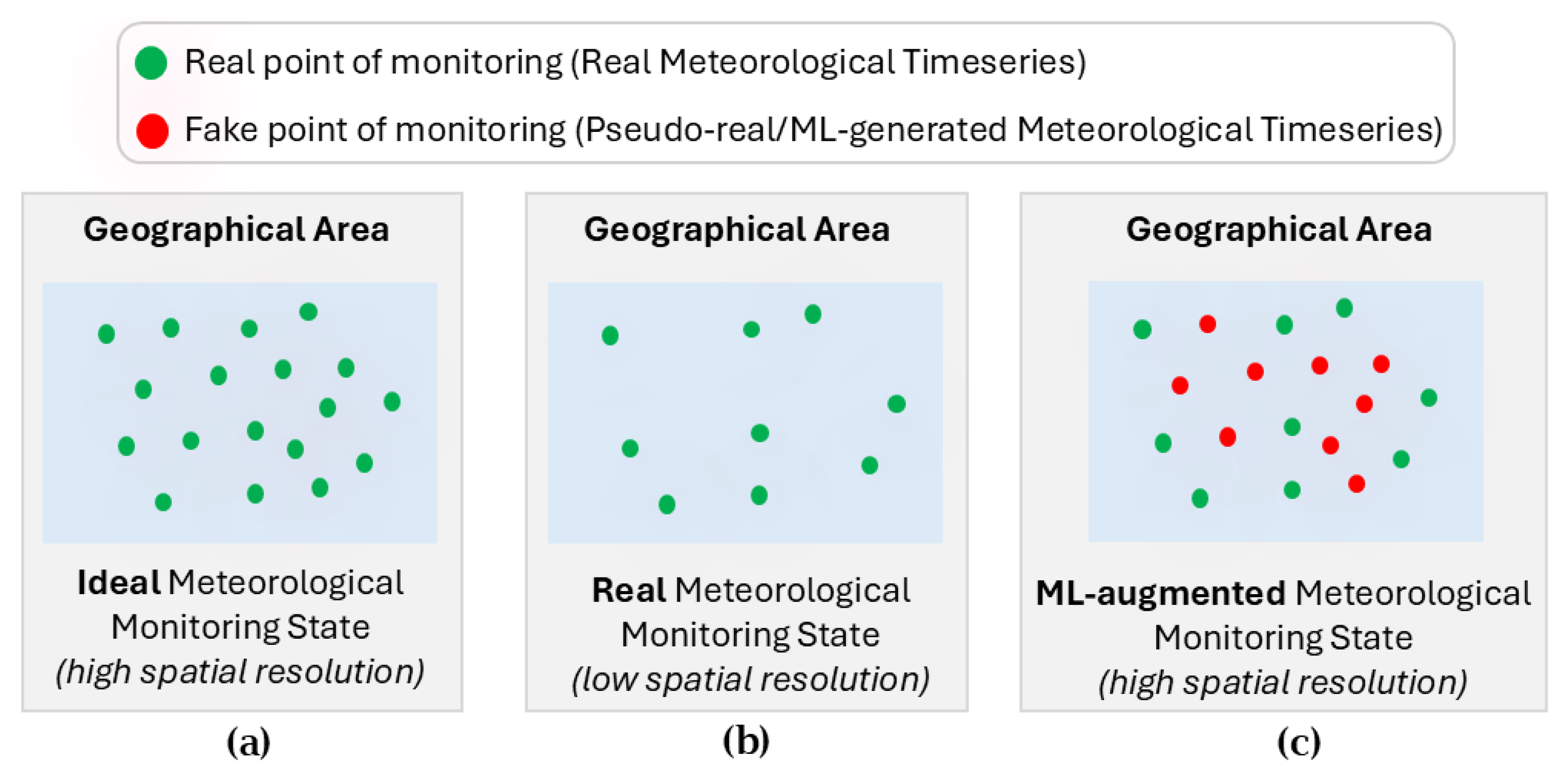
Figure 1. The idea of augmenting meteorological data monitoring in data-limited or data-free locations. (a) Ideal situation with dense deployment of meteorological stations. (b) Real situation with sparse deployment of meteorological stations. (c) Augmenting meteorological monitoring with pseudo-real (e.g., ML-predicted) data.
Jmse 13 02375 g001
Figure 2. Installation and telemetry system for remote data storage of the recordings at the pilot port.
Jmse 13 02375 g002
Figure 3. The geographical locations of the four reference points and the pilot port.
Jmse 13 02375 g003
Figure 4. Distribution of the wind speed components across the four reference points. Panels (ad) refer to reference points 1–4, respectively.
Jmse 13 02375 g004
Figure 5. Polar distribution (as wind rose diagrams) of the wind speed components across the four reference points. Panels (ad) refer to reference points 1–4, respectively.
Jmse 13 02375 g005
Figure 6. Partial Autocorrelation Function (PACF) of the wind speed vs. temporal lags across the four reference points. Panels (ad) refer to reference points 1–4, respectively.
Jmse 13 02375 g006
Figure 7. Occurrence frequency of different wind speed categories across the four reference points.
Jmse 13 02375 g007
Figure 8. General wind strength predictive framework for model training/inference.
Jmse 13 02375 g008
Figure 9. ML model structure for wind strength prediction based on current and historical values at the reference points (RPs).
Jmse 13 02375 g009
Figure 10. Schematic overview of the five ML models (MLR, DTR, SVR, RFR and GBR) used for supervised learning-based wind prediction at the pilot port. Each model follows different topologies and fitting methods to estimate function f ( x ( t ) ) . For simplicity, in each model, we consider univariate or bivariate representation of feature vector x ( t ) .
Jmse 13 02375 g010
Figure 11. Fitting performance of the deterministic models. Panels (ad) illustrate the actual versus the predicted wind timeseries derived by the SAM-last, SAM-sig, WAM-all, and WAM-sig models, respectively.
Jmse 13 02375 g011
Figure 12. Fitting performance of the ML models. Panels (ae) illustrate the actual versus the predicted wind timeseries derived by the MLR, DTR, SVR, RFR, and GBR, respectively.
Jmse 13 02375 g012
Figure 13. Prediction error in terms of MSE across different wind speed regression models, separately for (a) the short-horizon period (11-days predictions), and (b) the long-horizon period (8-months predictions).
Jmse 13 02375 g013
Figure 14. Prediction error in terms of MAE across different time lags, separately for (a) DTR model, and (b) GBR model.
Jmse 13 02375 g014
Figure 15. Importance scores for different input features (reference points and time lags), separately for (a) DTR model, and (b) GBR model.
Jmse 13 02375 g015
Table 1. ERA5 Dataset Summary.
Dataset ColumnDescriptionSize (Samples)
Timestamp (t)The timestamp of each sample in the form on year-month-day-hour473,352
Longitude (HGRS87 *)Longitude of reference points in HGRS87 system4
Latitude (HGRS87 *)Latitude of reference points in HGRS87 system4
Eastward wind speed ( u 10 )Wind speed values (m/s) along the x-axis473,352
Northward wind speed ( v 10 )Wind speed values (m/s) along the y-axis473,352
* Hellenic Geodetic Reference System 1987: the geodetic system commonly used in Greece (SRID = 2100).
Table 2. Multi-metric Performance Evaluation for the full-range wind series.
ModelMSEMAERMSEMAPE (%)R2WI (d)SFS
SAM-last0.940.740.97122.41−0.150.51−0.31
SAM-sig1.481.041.21184.91−0.800.55−1.33
WAM-all0.940.740.97122.17−0.150.51−0.29
WAM-sig0.940.740.97122.24−0.150.51−0.31
MLR0.750.640.86100.870.0850.35−1.19
DTR0.230.330.4836.710.710.910.75
SVR0.810.610.8982.080.0160.35−1.33
RFR0.350.430.5966.640.570.800.176
GBR2.14 × 10−50.00350.0051.170.970.960.96
Table 3. Multi-metric Performance Evaluation for the range-specific (high vs. low) wind series.
MetricWind Range * (ms)SAM-lastSAM-sigWAM-allWAM-sigMLRDTRSVRRFRGBR
MSELow0.721.450.720.720.460.180.440.222.12 × 10−5
High5.352.085.385.366.521.258.112.953.11 × 10−5
MAELow0.671.040.670.670.550.300.510.370.0034
High2.251.232.252.252.510.912.811.660.0037
RMSELow0.851.200.850.850.680.430.670.470.004
High2.311.442.322.312.551.122.851.720.005
MAPE (%)Low115.73182.63115.47115.5492.7827.4172.6957.911.11
High142.83197.66136.33136.31113.8739.7691.6971.221.81
* Wind Classes: (i) Low: Calm to light Breeze (0–3.3 m/s); (ii) High: gentle/strong Breeze (>3.3 m/s).
Disclaimer/Publisher’s Note: The statements, opinions and data contained in all publications are solely those of the individual author(s) and contributor(s) and not of MDPI and/or the editor(s). MDPI and/or the editor(s) disclaim responsibility for any injury to people or property resulting from any ideas, methods, instructions or products referred to in the content.