A Modified Leakage Localization Method Using Multilayer Perceptron Neural Networks in a Pressurized Gas Pipe


Department of Mechanical and Automotive Engineering, University of Ulsan, 93 Daehak-ro, Nam-Gu, Ulsan 44610, Korea
*
Author to whom correspondence should be addressed.
Appl. Sci. 2019, 9(9), 1954; https://doi.org/10.3390/app9091954
Submission received: 15 March 2019
/
Revised: 1 May 2019
/
Accepted: 8 May 2019
/
Published: 13 May 2019
(This article belongs to the Special Issue Ultrasonic Guided Waves)
Abstract
:Featured Application
To improve the leakage location accuracy in a pressurized gas pipe, this paper proposes a modified leakage location method using multilayer perceptron neural networks based on the acoustic emission signal.
Abstract
Leak detection and location in a gas distribution network are significant issues. The acoustic emission (AE) technique can be used to locate a pipeline leak. The time delay between two sensor signals can be determined by the cross-correlation function (CCF), which is a measure of the similarity of two signals as a function of the time delay between them. Due to the energy attenuation, dispersion effect and reverberation of the leakage-induced signals in the pipelines, the CCF location method performs poorly. To improve the leakage location accuracy, this paper proposes a modified leakage location method based on the AE signal, and combines the modified generalized cross-correlation location method and the attenuation-based location method using multilayer perceptron neural networks (MLPNN). In addition, the wave speed was estimated more accurately by the peak frequency of the leakage-induced AE signal in combination with the group speed dispersive curve of the fundamental flexural mode. To verify the reliability of the proposed location method, many tests were performed over a range of leak-sensor distances. The location results show that compared to using the CCF location method, the MLPNN locator reduces the average of the relative location errors by 14%, therefore, this proposed method is better than the CCF method for locating a gas pipe leak.
1. Introduction
Pipelines are used to transport natural gas, water, oil products and other easy-flowing products, and pipeline leakage is a common phenomenon in the continuous transportation process due to the corrosion of pipe walls [1], third-party interference [2], aging of the pipes [3], etc. Leakage may lead to environmental pollution, energy loss, injuries, and even fatalities. Therefore, leakage location is one of the paramount concerns of pipeline operators and researchers.
Pipeline leakage detection methods include direct and indirect methods [4]. Direct methods detect the leaked product outside the pipeline using fiber optic sensing, moisture measurements, gas tracing, vapor sensing, etc. [5]; however, these methods suffer from low sensitivities and expensive sensors. Indirect methods detect the leakage by measuring the pipeline gas pressure, flow, temperature, etc. using sensors mounted inside the pipeline; however, many pressurized vessels in industry are inaccessible, which necessitates nondestructive testing. Acoustic emission (AE) [6] is a nondestructive testing technique that provides the ability to rapidly locate small-scale leaks [7]; it has thus now become a common leak location method. AE signals can be generated by friction, cavitation, impact, or leakage in a high-pressure pipe. In this study, the AE signals in the pipe wall are detected by AE sensors mounted on the pipe’s exterior surface.
Leakage location commonly relies on attenuation-based methods or time-of-flight-based methods [8]. The former methods are based on the reduction in the AE signal strength as the propagation distance increases. The prerequisite for the latter methods is that the wave speed is a known constant; however, the wave speed varies as a function of frequency due to the group speed dispersion nature of gas-leakage-induced guided waves [9]. To determine the speed of the AE signal, Li et al. [10] derived the wavenumber formulae to predict the wave speeds, and thereby halved the location error compared to that using the theoretical wave speed. Davoodi and Mostafapour [11] derived the motion equation of the pipe for the simply supported boundary condition by the standard form of Donnell’s nonlinear cylindrical shell theory. Nishino et al. [12] generated wide-band cylindrical waves in aluminum pipes by the laser-ultrasonic method; the experimental results showed good agreement between the theoretical and experimental group speed dispersion curves. In this study, the group speed of the leakage-induced signal was estimated by its peak frequency in combination with the group speed dispersive curve of the fundamental flexural mode.
When leakage-induced signals transmit along the pipe wall, signal distortion arises due to energy attenuation, dispersion effect [13] and reverberation. The cross-correlation function (CCF) can determine the time delay based on the similarity of two signals. However, the degree of signal distortion affects the similarity of two signal waveforms measured by two AE sensors, and this interference degrades the performance of the CCF method. To improve the leakage location accuracy, Davoodi and Mostafapour [14,15] located a leak on a high-pressure gas pipe by wavelet transform, filtering technique, and CCF. Yu et al. [16] located the leakage by dual-tree complex wavelet transform and singular value decomposition. Brennan et al. [17] estimated the time delay between two channels by the time and frequency domain methods, with almost identical test results being obtained. Sun et al. [18] proposed a leakage aperture recognition and location method using the root mean square entropy of local mean deposition and Wigner-Ville time-frequency analysis. Guo et al. [19] proposed an adaptive noise cancellation method using the empirical mode decomposition, the test result showed that the time delay estimation of the leakage-induced signal is more accurate. Yang et al. [20] estimated the characteristics related to the two propagation channels by blind system identification. The travel duration of the leakage source signals from the leak point to either sensor was extracted from the identified propagation channel. This paper proposes a modified generalized cross-correlation (GCC) location function, which can compensate for the weakening effect of the different propagation paths on the leakage-induced signals. After the multilayer perceptron neural networks (MLPNN) is trained by the distances between the impact points and the sensors and the energy ratios of two impulse response signals measured by two sensors, it can obtain the relationship between the signal energy ratios and the vibration excitation location, and thus can locate a pipeline leak. This location method can be used to locate a leak in a pipe made of isotropic materials, such as metallic, plastic, etc., whose elastic modulus, Poisson’s ratio and density of which should be constant. In this paper, the impulse response signals are generated by the collision between an impulse hammer and the pipe.
Although the proposed method is applicable for pipes with variable operating pressure, this study only deals with the location of a single leak source when the gas pressure inside the pipe is constant. The rest of this paper is organized as follows. Section 2 introduces the modified GCC location method and wave speed estimation based on modal analysis of gas-leakage-induced guided waves. Section 3 introduces the principle of the leak location method based on the AE signal energy attenuation and the MLPNN. Section 4 presents the experimental setup, data collection and the signal processing for leakage location. Section 5 analyzes the experiment results. Section 6 presents the study conclusions.
2. The Principle of Leak Location Method Based on the Generalized Cross-Correlation Function
2.1. The Modified Generalized Cross-Correlation Location Method
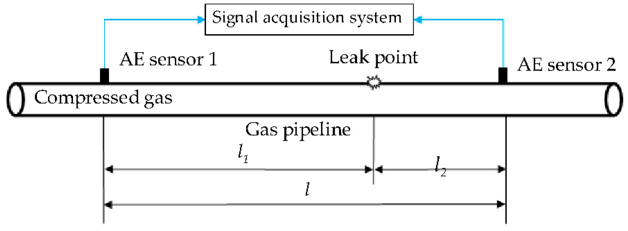
Figure 1 presents a pressurized piping system: l is the distance between the two sensors, and l1 and l2 are the distances between the leak point and sensors 1 and 2, respectively.
If there is a leak between the two AE sensors, the two measured signals x1(t) and x2(t) can be mathematically modeled [21] as
where s(t) is the leakage-induced signal measured at the leak location, the parameter t is the discrete-time counter, and d denotes the time delay between two measured signals. h1(t) and h2(t) are the discrete-time impulse response functions between the leak point and each sensor, respectively, and they provide the relationships between an impulse signal and each sensor signal. n1(t) and n2(t) are the background noises picked up by the two sensors, is the discrete-time convolution operator. s(t), n1(t) and n2(t) are assumed as stationary random signals. The noises measured by the two sensors are assumed to be mutually unrelated and unrelated with the leakage-induced signal, so the CCF between two measured signals with noise and without noise are equivalent, and can be expressed as follow:
where Rs1s2(τ) and Rx1x2(τ) are the CCF without noise and with noise, respectively, in terms of the time delay τ. Since the CCF is sensitive to the non-leak vibration noises [21], the time delay is commonly estimated by the GCC function [22], which can be written as:
where F−1{·} denotes the inverse discrete Fourier transform, ω denotes the frequency, and Ψg(ω) is the frequency weighting function of the GCC function. Sx1x2(ω) is the cross-spectral density between two measured signals x1(t) and x2(t) [23], and can be written as:
where E[·] denotes the expectation operator, X1(ω) and X2(ω) are the N-point discrete Fourier transforms (DFT) of x1(t) and x2(t), respectively, H1(ω) and H2(ω) are the DFT of h1(t) and h2(t), respectively, Sss(ω) is the auto-spectral density of s(t), and (·)* means complex conjugation. Since multiplication in the frequency domain corresponds to convolution in the time domain [24], the GCC function between two measured signals in terms of the time delay τ can be derived by substituting Equation (4) into Equation (3), and expressed as:
where Rll(τ) = F−1{Sss(ω)} is the autocorrelation function of s(t), and Ψg(τ) = F−1{Ψg(ω)|H1*(ω)H2(ω)|}, δ (τ + d) = F−1{eiωd}. The time delay between two measured signals is equal to the quotient of the offset of the GCC maximum peak and the sampling frequency. δ (τ + d) is a function equal to zero everywhere except for τ = −d, and the Dirac Delta function’s integral over the entire real line is equal to one. If Ψg(ω) = 1, the Dirac delta function δ (τ + d) delayed by d will be broadened by Sss(ω), H1(ω) and H2(ω) [25]. In fact, Sss(ω) is often unknown as it depends on the leakage aperture, the gas pressure difference between inside and outside the pipe [10], etc. However, H1(ω) and H2(ω) can be obtained by the impulse response method [26], and can be calculated by using:
where the parameter i indicates the sensor serial number, Yi(ω) denotes the DFT of the impulse response signal measured by the corresponding sensor, and X(ω) is the DFT of the impulse signal measured by the impact hammer. In this study, the impulse signal is assumed as the Dirac delta function. Therefore, to compensate for the weakening effect of the pipes on the AE signals, the modified frequency weighting function of the GCC function is written as:
The modified GCC function Rx1x2g(τ) can be derived by substituting Equations (4) and (7) into Equation (3), and expressed as:
Compared with Equation (5), pre-filter Ψg(ω) removes the effects of the propagation paths on the AE signal, δ (τ + d) is only broadened by Sss(ω). Therefore, the modified frequency weighting function can increase the degree of correlation between two measured signals and improve the accuracy of the time delay estimation. The modified frequency weighting function differs from the PHAT processor function [25] in that the frequency weighting function involves pre-whitening of the leakage-induced signal. To reduce the effects of noise on the time delay estimation, only the leakage-induced signal with greater power spectral density should be extracted and processed by the proposed pre-filter.
Figure 2 shows a schematic of the modified GCC location method, which contains N-point DFT, complex conjugate, cross power spectrum, pre-filter and N-point inverse discrete Fourier transform (IDFT).
The leakage can be located by:
where l is the distance between the two sensors, lest is the estimated distance between the leak and one sensor, and dest is the time delay estimation. The frequency-dependent speed v(ω0) [9] of AE signals along the pipe wall is discussed in Section 2.2. In this study, the relative location error with respect to the distance between the leak and one sensor is determined as:
The cross-correlation coefficient (CCC) [27] in terms of the time delay τ can be used to evaluate the correlation of two measured signals and it is given by:
where Rx1x1(0) and Rx2x2(0) are the amplitudes in the autocorrelation functions of x1(t) and x2(t), respectively, for τ = 0. The larger the maximum peak in CCC is, the higher the degree of the correlation between the two signals is [28].
2.2. Wave Speed Estimation Based on Modal Analysis of Gas-Leakage-Induced Guided Waves
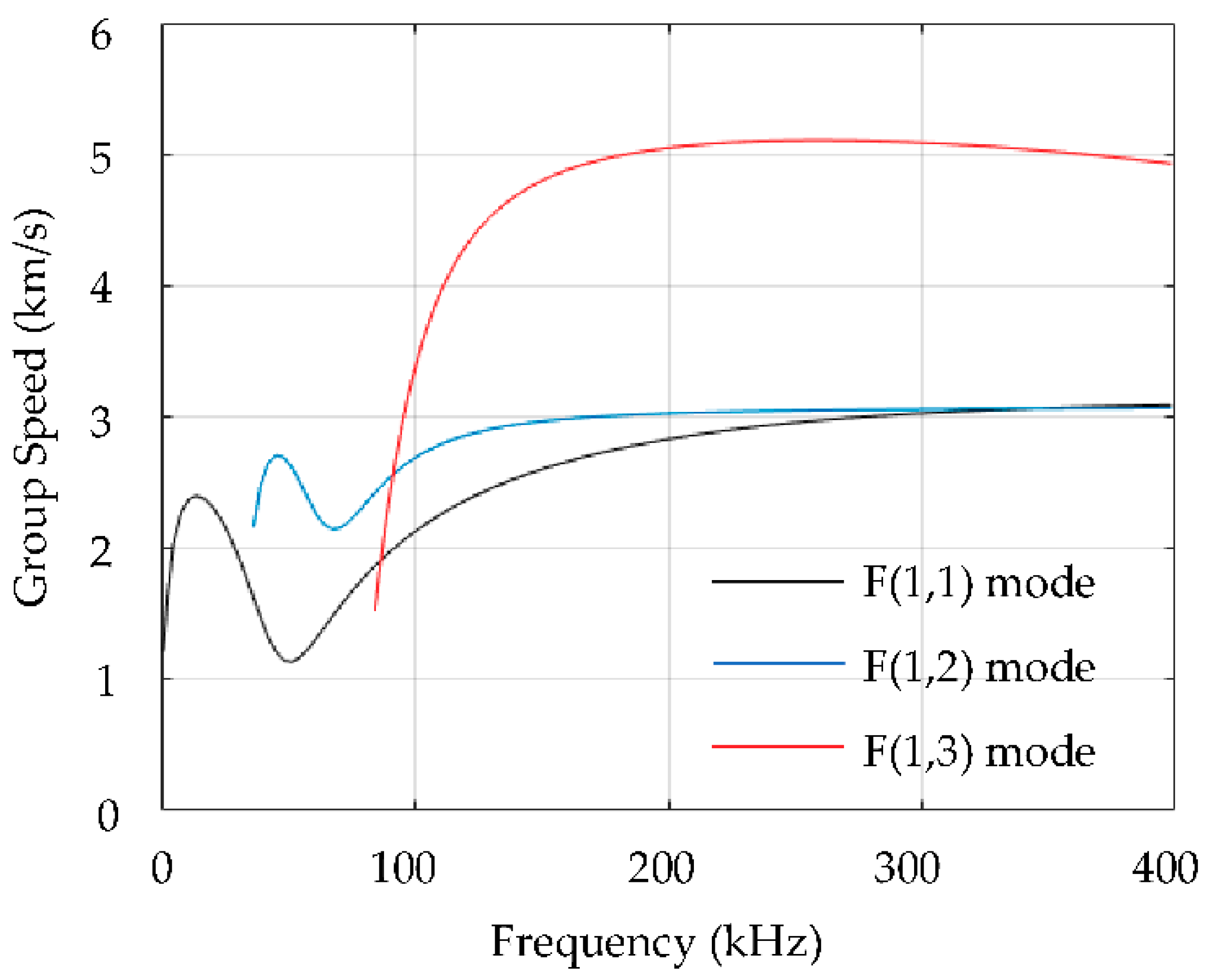
Since the gas solid coupling between the in-pipe gas and the pipe wall can be ignored due to the acoustic impedance mismatch between them, the gas-filled pipes can be approximated as hollow cylinders [9]. The dispersive behaviors of the guided waves in a gas pipe can be analyzed by the guided wave theory of the hollow cylinders [29]. The guided waves in a pipe are grouped into three families: longitudinal mode, torsional mode, and flexural mode. These modes are denoted by L(0,m), T(0,m) and F(n,m), respectively, where n and m represent the circumferential and radial modal parameters, respectively. The theoretical analysis shows that the radial vibration signal collected by AE sensors is dominated by the dispersive fundamental flexural mode F(1,1) [30].
If the material of the pipe wall is changed, the group speed dispersive curve needs to be calculated again based on some parameters before determining the group speed of the leak-induced signal, those parameters are external diameter, thickness, elastic modulus, Poisson’s ratio and density of the pipe wall. The material and geometric parameters of the given pipe are shown in Table 1. According to the parameters of the given pipe, the group speed dispersive curves of the flexural modes shown in Figure 3 can be obtained using the guided wave theory of hollow cylinders in MATLAB R2018b. The speed of the AE signal can be online estimated by the peak frequency of the AE signal in combination with the known group speed dispersive curve of the fundamental flexural mode [9].
3. The Principle of the Leak Location Method Based on the AE Signal Energy Attenuation
3.1. AE Signal Energy Attenuation
The energy of the AE signal reduces as the propagation distance increases due to geometric spreading, structural scattering, and energy absorption [14]. The weakening effect of the pipe on AE signals is similar with the low-pass filter [10], in that the cut-off frequency decreases as the propagation distance increases. When the AE signals propagate in one direction along the pipe wall, the energy attenuation of the AE signal can be described by an exponential decay [31]:
where E is the energy of the sensor signal, E0 is the AE signal energy at the leak point and k is the attenuation coefficient. The AE signal energy is proportional to the integral of the square of the signal amplitude [32], and can be written as:
where ∆T represents the length of sample time in seconds, and v represents the instantaneous signal amplitude in voltages. If the distance between the vibration source and the sensor is constant, the weakening effect of the pipe on the AE signal will be also constant, irrespective of any leakage-induced signals or impulse response signals. The closer the sensor is to the leak source, the greater the energy of the measured signals. Then the energy ratios of two measured signals will gradually increase or decrease as the distance between the vibration source and one of the two sensors increases. Therefore, a pipeline leakage can be located by the signal energy ratios without knowing the wave speed or the time delay estimation.
3.2. Multilayer Perceptron Neural Networks Classifier
The mathematical model of the biological neural network is defined as the artificial neural network [33]. The relationships between the input and output vectors can be obtained after the artificial neural networks are trained. Neural network can be applied to solve nonlinear problems, MLPNN is a commonly used model. Figure 4 shows the perceptron neural networks with three layers. The input and output layers accept the external input vectors in the learning mode. Every neuron in the input and hidden layers connects to every neuron in the hidden and output layers, respectively. The input layer L1 is comprised of P variables x = [x1, ···, xP]T, which are processed by the following equation:
where M is the number of neurons in the hidden layer, and the superscript indicates that the parameter ωij(1) is the connection weight between the neuron xi in the input layer L1 and the neuron zj in the hidden layer L2. The parameter ω0(1) represents the bias of the variable aj, which prevents aj from becoming zero. Then aj is transformed by an activation function, which is the logistic sigmoid function in this study, and it is given by:
Similarly, the neuron y in the output layer L3 receives the variables zj as shown in the following equation:
where ωj(2) and ω0(2) are the connection weight and the bias in the hidden layer, respectively. For the regression problem, the aim of the training process is to minimize the squared error function as shown in the following equation by the gradient descent method:
where d is the distance between the vibration source and one sensor, ω is the set of all weights and biases, and y(ω) represents the neuron in the output layer. All the weights and biases need to be updated by training the MLPNN on labeled data until the error function becomes small enough or the maximum iteration is reached; then the MLPNN can be used as a leakage locator.
4. Laboratory Experiments
4.1. Experimental Setup and Data Collection
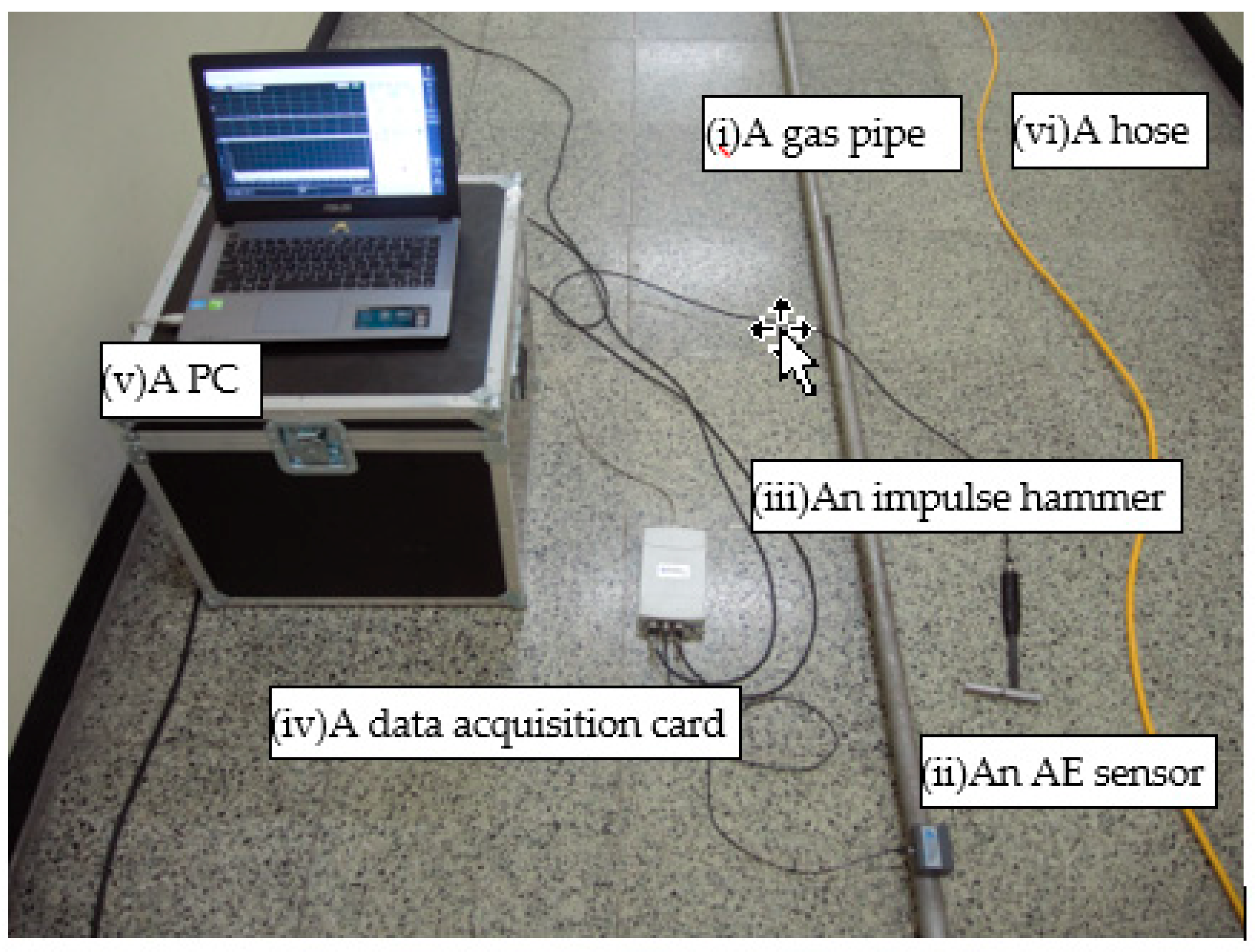
The experimental setup consists of two parts: a pressurized piping system and a signal acquisition system, as shown in Figure 5. If the pipe gas pressure is too low, the energy of the leak-induced signal will be small and difficult to detect. Therefore, in the pressurized piping system, an air compressor (NH-5, Hanshin product) supplies 7 bar gas pressure to a 15m-long steel pipe (ASTM A 312 TP304) with a pipe wall thickness and external diameter of 2.8 mm and 33.4 mm, respectively. One end of the pipe was blocked, and the other end was connected to the air compressor via a hose. To avoid the air compressor vibration noise affecting the experimental results, the air compressor was placed far away from the piping system. The pipe was supported by a sponge material to reduce energy dissipation of the AE signal on the pipe wall to the ground. The diameter of the leakage orifice in the early stage of a pipeline leakage is usually small. To verify that the proposed method can locate a leak in this stage, a simulated leak orifice with a diameter of 0.3 mm was punched in the pipe wall. The simulated leak source, the AE sensor mounted on the pipe wall, an impulse hammer and the placement of two AE sensors along the pipe are shown in Figure 6, Figure 7, Figure 8 and Figure 9, respectively. The pipe wall had been cleaned with sandpaper before the AE sensors were mounted with the magnetic hold downs and vacuum grease couplant.
The signal acquisition system consists of two R15a sensors with a resonant frequency of 150 kHz, an impulse hammer (086C03), a data acquisition card (USB-5132, NI product) and a personal computer (PC) equipped with NI-SCOPE software. Since the sensitivity of the AE sensors is high in the frequency range between 50 kHz and 400 kHz, data were captured at a sampling rate of 800 kHz in the experiment. Analog to digital conversion was performed by the data acquisition card connected to the PC. Data were recorded into the PC for the signal processing and preprocessed by the NI-SCOPE software, including the preamplification and anti-aliasing filtering.
In the experiment, the training sets for MLPNN include the distances between one sensor and each impact location and the impulse response signals energy ratios between two sensor signals in different frequency bands. The impulse signal was measured by the sensor in the impact hammer, and the impulse response signals were measured by AE sensors when the pipe was tapped by the impact hammer, and the tapping locations were distributed along a straight line between the two AE sensors. To avoid the simulated leak orifice affecting the impulse response signal, the impact test was performed before the simulated leak orifice was punched. The test sets for MLPNN were the energy ratios of leakage-induced signals in different frequency bands. The leakage-induced signals were generated by the friction force between the jet of the leaking gas and the simulated leak orifice.
4.2. Signal Processing for Leakage Location
The leakage location procedure for the MLPNN locator is shown in Figure 10, and the MLPNN locator operates in two different modes:
- 1. In the learning mode, the training sets of the MLPNN contain the input vectors and the output vectors. The input vectors are the energy ratios of two impulse response signals in corresponding frequency bands. Since the impulse response signals are non-stationary signals, and the wavelet packet analysis is suitable for processing the non-stationary signals, then the impulse response signals were processed by the wavelet packet transform in this study. The output vectors are the distances between one sensor and each impact location. The learning procedure for the MLPNN is as follows:
- Since the energy of a leakage-induced signal at frequency band from 100 to 150 kHz is higher than at other frequency bands, and three-level decomposition can extract the signal in this frequency range, so all the impulse response signals are decomposed into three layers of wavelet packet coefficients, and the signals are reconstructed in eight frequency bands by wavelet packet coefficients. The Haar wavelet is used in this study.
- Calculate the energies of the decomposed signals in step 1 by Equation (13); then calculate the energy ratios of two impulse response signals in the corresponding frequency band.
- Train the MLPNN with the input and output vectors. The input vectors are the energy ratios in step 2, and the output vectors are the distances between one sensor and each impact location, and the epochs in the training method is set to 0.01.
- 2. In the application mode, the trained MLPNN locator can locate the leakage by using the energy ratios of the leakage-induced signals in the frequency bands with greater power spectral density. The leakage location procedures for the MLPNN locator are described as follows:
- Measure the leakage-induced signals by using the two AE sensors.
- Determine the peak frequency of the leakage-induced signals by using the power spectral density.
- Estimate the group speed of the leakage-induced signals by using the peak frequency in step 2 and the known group speed dispersive curve of the fundamental flexural mode.
- Calculate the CCC by using the CCF method and the modified GCC method.
- Compare the maximum peak amplitudes of the two CCCs obtained in step 4. ρx1x2c and ρx1x2g are the maximum peak amplitudes of the CCCs obtained by using the CCF method and the modified GCC method, respectively. If ρx1x2g is greater than ρx1x2c, it implies that compared to the CCC obtained by using CCF method, the CCC obtained by using modified GCC method is more reliable; then perform step 6, otherwise perform step 7.
- Calculate the distance between the leakage and sensor 1 by Equation (9). The group speed of the leakage-induced signal was determined in step 3, and the time delay was determined by the sampling frequency and the offset of the CCC maximum peak obtained by the modified GCC method in step 4.
- Decompose the leakage-induced signals into three layers wavelet packet coefficients, reconstruct the signals in eight frequency bands by using the wavelet packet coefficients.
- Calculate the energy ratios of the decomposed signals in the frequency bands with the greater power spectral density.
- Locate the leakage by using the energy ratios in step 8 and the trained MLPNN locator.
5. Results and Discussion
5.1. Characteristics of the Frequency Domain
Figure 11 shows the power spectral densities of the leakage-induced signals collected at the distances of 1 m and 2 m away from the simulated leak source. The center frequency of a leak-induced signal is proportional to the gas jet velocity and inversely proportional to the leakage aperture [10], and is also related to the resonant frequency of the sensor and the propagation distance between the leak and the sensor. As shown in Figure 11, the amplitude of the power spectral density decreases with increasing propagation distance. Since the peak frequency of leakage-induced signals is 124 kHz, the wave speed can be determined to be 2404 m/s by the peak frequency in combination with the known group speed dispersive curve of the fundamental flexural mode.
5.2. Characteristics of the Signal Energy Ratios
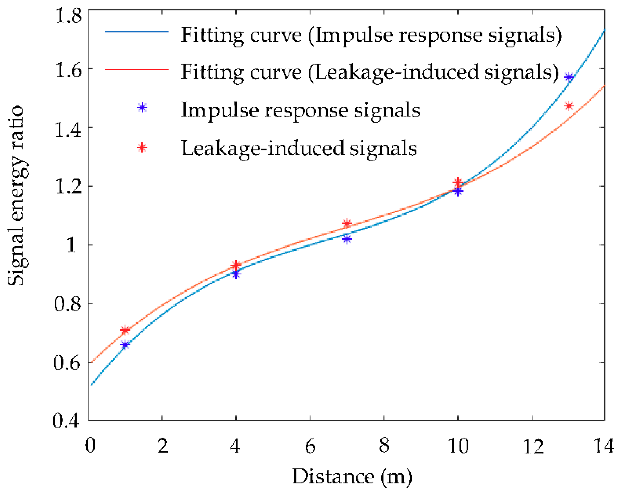
To verify the consistency of weakening effect of the pipe on two kinds of signals, which are the impulse response signals and leakage-induced signals measured by maintaining a distance of 14 m between the two sensors while varying the distance between sensor 1 and the simulated leak orifice. Since the maximum amount of leakage-induced signal energy occurs in frequencies near 124 kHz, the signal-to-noise ratio at this frequency band is higher than at other bands, the impulse response signal in frequencies near 124 kHz was also extracted with wavelet packet transform, and the signal energy ratios between the two sensors were calculated. Figure 12 shows the fitting curves of the signal energy ratios as a function of the propagation distance. The horizontal axis denotes the distance between sensor 1 and the simulated leak orifice. The vertical axis denotes the energy ratios of the leakage-induced signal and the impulse signal measured by the two sensors. The difference between the two fitting curves is small, which implies that the weakening effect of the pipe on the AE signals is proportional to the propagation distance, irrespective of any leakage-induced signals or impulse response signals. Therefore, the signal energy ratio can also be used for locating the vibration excitation source.
5.3. Characteristics of the Time Domain.
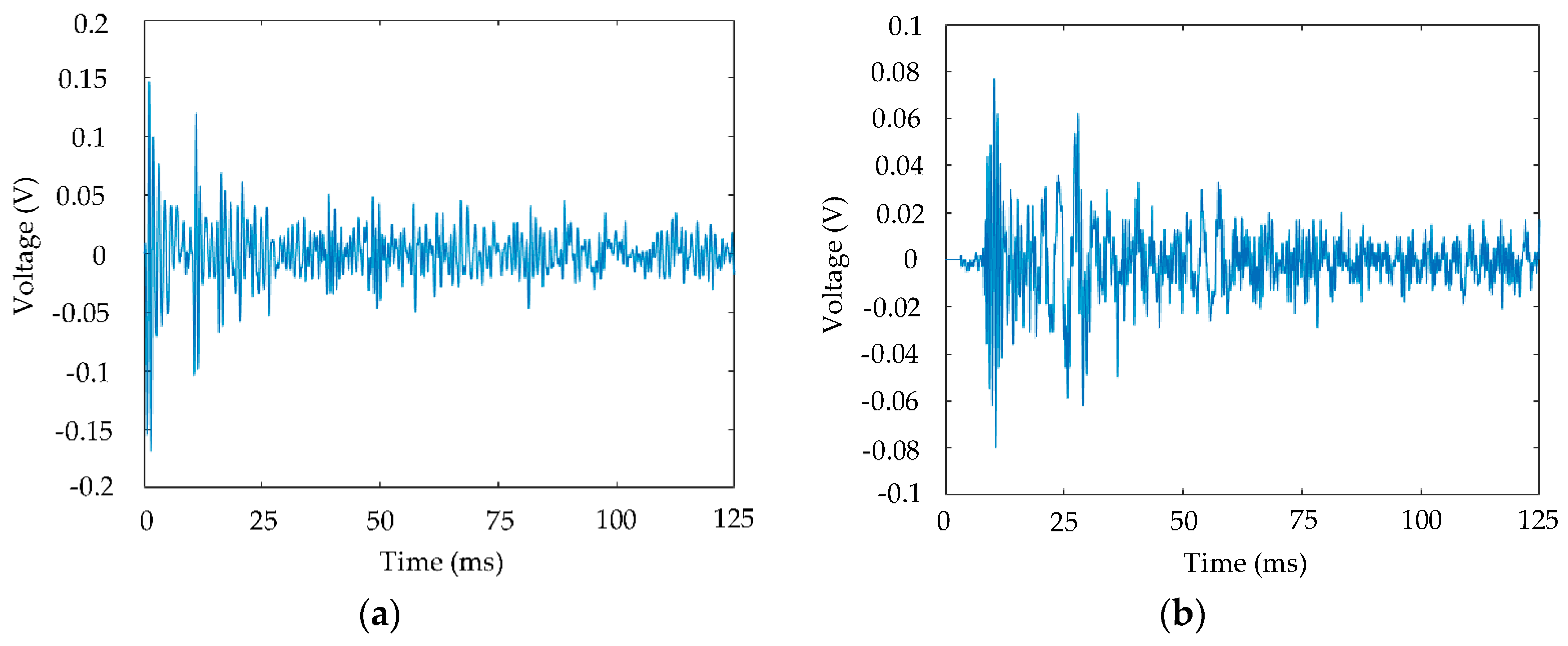
Figure 13a,b show the impulse response signals collected at distances of 0.4 m and 13 m away from the impact location, respectively. The maximum amplitude of the impulse response signals decreases as the propagation distance increases, which indicates that the energy of the impulse response signal decreases due to energy attenuation. Moreover, the closer the vibration source is to the sensor, the earlier the impulse response signal begins to oscillate.
Figure 14a,b show the CCC obtained by the CCF method and the modified GCC method, respectively. The time delay estimation only depends on the shift value of the maximum peak in the cross-correlation coefficient with respect to the central point, and can be calculated as the product of the sampling period and the shift of the cross-correlation function maximum peak [34]. Two maximum peaks can be observed, and the time delay estimations are −0.00020 seconds and −0.00034 seconds, respectively. The distance estimations between the leak and sensor 1 are 1.83 m and 1.99 m, respectively. Since the relative location error in this study is equal to the quotient of the leakage location error and the distance between the leak and sensor 1, the real distance between the simulated leak orifice and sensor 1 is 2.16 m, so the relative location errors are 15% and 8%, respectively. The maximum peak amplitudes of the two CCCs are 0.168 and 0.236, respectively. Hence, the modified pre-filter can improve the accuracy of the time delay estimation and increase the degree of the correlation between the two measured signals.
5.4. Leakage Location Analysis
To verify the reliability of the MLPNN locator, the gas leakage was located by the CCF location method and the MLPNN locator under different conditions, which are maintaining a distance of 2.16 m between the simulated leak orifice and sensor 1 and varying the distance (1.08 m, 2.36 m and 3.54 m) between the simulated leak orifice and sensor 1. In addition, the group speed of the leakage-induced signal was determined by the peak frequency of the leakage-induced signal and the group speed dispersive curve of the fundamental flexural mode. Table 2 and Table 3 show the location results obtained by the CCF method and the MLPNN locator. The relative location errors in Table 3 show that the relative location errors increase as the distance between the two sensors increases, which implies that some high frequency components of the leakage-induced signal attenuate as the propagation distance increases.
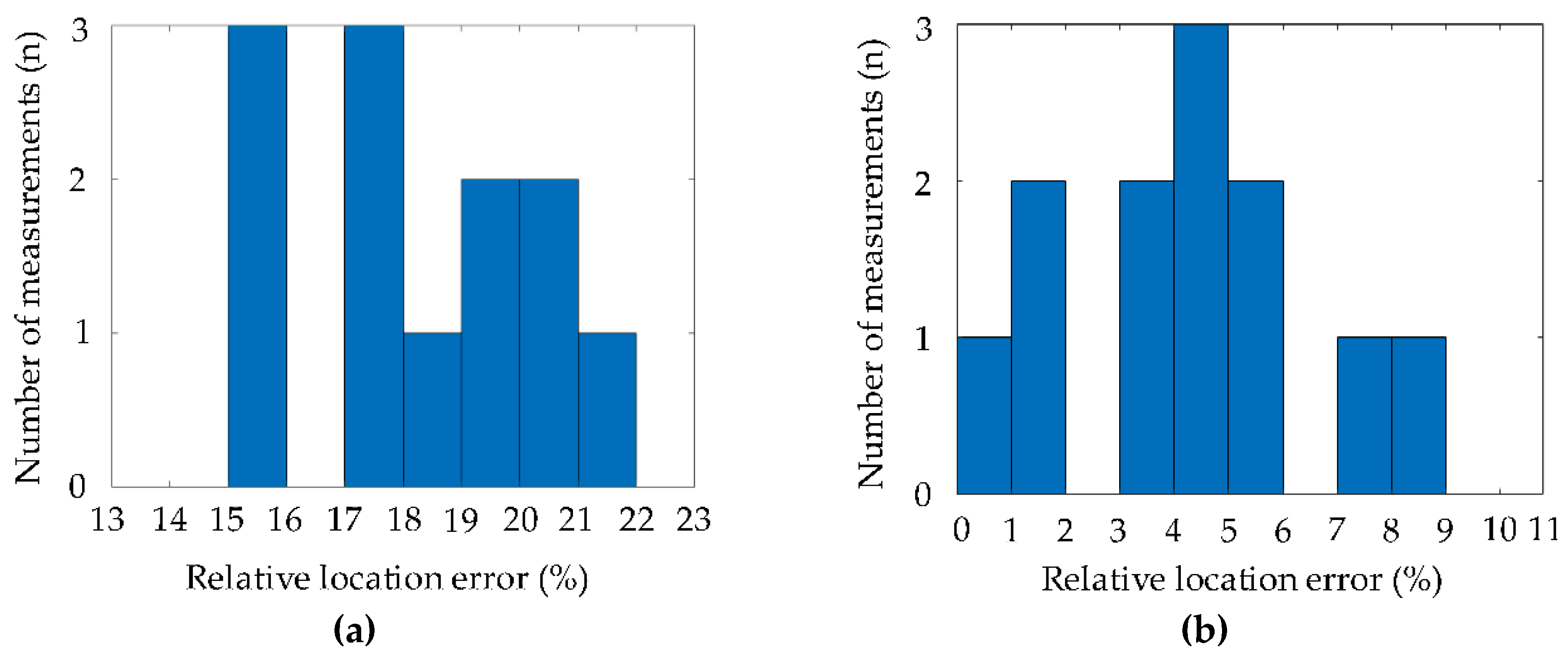
Figure 15a,b show the histograms of the relative location errors in Table 2 and Table 3, respectively. The vertical axis represents the number of measurements, and the horizontal axis represents the percentage of relative location error. These two tables show the measurement results of twelve groups by using the proposed method and the cross-correlation function, respectively, with twelve measurements in both Figure 15a,b. Despite the small sample size, all the measurement results are typical and can show the location accuracy of the two location methods. The averages of the relative location errors are 18% and 4%, respectively, which indicates that the average of the relative location errors obtained by the MLPNN locator is reduced by 14% compared to that using the CCF location method. Consequently, the MLPNN locator is more suitable for locating a leak in a gas pipe than the CCF location method is. However, the MLPNN locator suffers the drawback of needing to be trained again if one of the following experimental conditions changes: for example, the distance between the two AE sensors, the geometric parameters of the pipe wall, or the material of the pipe wall.
6. Conclusions
This paper has proposed a leakage location method using the modified generalized cross-correlation (GCC) location method in combination with the attenuation-based location method using multilayer perceptron neural networks (MLPNN). The GCC location method can compensate for the weakening effect of the different propagation paths on the leakage-induced signals, can increase the degree of the correlation between two measured signals and improve the accuracy of the time delay estimation. Unlike the cross-correlation function (CCF) location method, the MLPNN locator locates a leak not only by the time delay estimation between two measured signals but also by the energy ratios of two leakage-induced signals measured by two sensors in the frequency bands with greater power spectral density. In addition, the wave speed was determined more accurately by using the peak frequency in combination with the group speed dispersive curve of the fundamental flexural mode. The MLPNN locator was experimentally verified by using a pressurized piping system and a signal acquisition system. The average of the relative location errors obtained by the MLPNN locator was reduced by 14% compared to that using the CCF location method. Hence, the MLPNN locator is more suitable for locating a leak in a gas pipe than the CCF location method is.
Data Availability
The data used to support the findings of this study are available from the corresponding author upon request.
Author Contributions
Conceptualization, C.-M.L.; methodology, Q.W. and C.-M.L.; software, Q.W.; validation, Q.W.; formal analysis, Q.W.; investigation, Q.W.; resources, C.-M.L.; data curation, X.X.; writing—original draft preparation, Q.W.; writing—review and editing, Q.W.; visualization, Q.W.; supervision, C.-M.L.; project administration, C.-M.L.; funding acquisition, C.-M.L.
Funding
This research was funded by a 2017 grant from the Russian Science Foundation (Project No. 17-19-01389).
Conflicts of Interest
The authors declare no conflicts of interest.
References
- Edalati, K.; Rastkhah, N.; Kermani, A.; Seiedi, M.; Movafeghi, A. The use of radiography for thickness measurement and corrosion monitoring in pipes. Int. J. Press. Vessels Pip. 2006, 83, 736–741. [Google Scholar] [CrossRef]
- Liang, W.; Hu, J.; Zhang, L.; Guo, C.; Lin, W. Assessing and classifying risk of pipeline third-party interference based on fault tree and SOM. Eng. Appl. Artif. Intell. 2012, 25, 594–608. [Google Scholar] [CrossRef]
- Vargas-Arista, B.; Hallen, J.M.; Albiter, A. Effect of artificial aging on the microstructure of weldment on API 5L X-52 steel pipe. Mater. Charact. 2007, 58, 721–729. [Google Scholar] [CrossRef]
- Ferraz, I.N.; Garcia, A.C.; Bernardini, F.C. Artificial Neural Networks Ensemble Used for Pipeline Leak Detection Systems. In Proceedings of the 7th International Pipeline Conference IPC 2008, Calgary, AB, Canada, 29 September–3 October 2008; pp. 739–747. [Google Scholar]
- Nehorai, A.; Paldi, E.; Porat, B. Detection and Localization of Vapor-Emitting Sources. IEEE Trans. Signal Process. 1995, 43, 243–253. [Google Scholar] [CrossRef]
- Xiao, Q.; Li, J.; Bai, Z.; Sun, J.; Zhou, N.; Zeng, Z.A. Small Leak Detection Method Based on VMD Adaptive De-Noising and Ambiguity Correlation Classification Intended for Natural Gas Pipelines. Sensors 2016, 16, 2116. [Google Scholar] [CrossRef] [PubMed]
- Faerman, V.A.; Cheremnov, A.G.; Avramchuk, V.V.; Luneva, E.E. Prospects of Frequency-Time Correlation Analysis for Detecting Pipeline Leaks by Acoustic Emission Method. IOP Conf. Ser. Earth Environ. Sci. 2014, 21, 012041. [Google Scholar] [CrossRef] [Green Version]
- Rewerts, L.E.; Roberts, R.R.; Clark, M.A. Dispersion compensation in acoustic emission pipeline leak location. In Review of Progress in Quantitative Nondestructive Evaluation; Springer: Boston, MA, USA, 1997; Volume 16, pp. 427–434. [Google Scholar]
- Li, S.; Wen, Y.; Li, P.; Yang, J.; Dong, X.; Mu, Y. Leak location in gas pipelines using cross-time-frequency spectrum of leakage-induced acoustic vibrations. J. Sound Vib. 2014, 333, 3889–3903. [Google Scholar] [CrossRef]
- Li, S.; Wen, Y.; Li, P.; Yang, J.; Yang, L. Determination of acoustic speed for improving leak detection and location in gas pipelines. Am. Inst. Phys. 2014, 85, 024901. [Google Scholar] [CrossRef]
- Davoodi, S.; Mostafapour, A. Modeling Acoustic Emission Signals Caused by Leakage in Pressurized Gas Pipe. J. Nondestruct. Eval. 2013, 32, 67–80. [Google Scholar] [CrossRef]
- Nishino, H.; Takashina, S.; Uchida, F.; Takemoto, M.; Ono, K. Modal analysis of hollow cylindrical guided waves and applications. Jpn. J. Appl. Phys. 2001, 40, 364–370. [Google Scholar] [CrossRef]
- Grabec, I. Application of correlation techniques for localization of acoustic emission sources. Ultrasonics 1978, 16, 111–115. [Google Scholar] [CrossRef]
- Davoodi, S.; Mostafapour, A. Gas leak locating in steel pipe using wavelet transform and cross-correlation method. Int. J. Adv. Manuf. Technol. 2013, 70, 1125–1135. [Google Scholar] [CrossRef]
- Mostafapour, A.; Davoodi, S. Leakage Locating in Underground High Pressure Gas Pipe by Acoustic Emission Method. J. Nondestruct. Eval. 2012, 32, 113–123. [Google Scholar] [CrossRef]
- Yu, X.C.; Liang, W.; Zhang, L.B.; Jin, H.; Qiu, J.W. Dual-tree complex wavelet transform and SVD based acoustic noise reduction and its application in leak detection for natural gas pipeline. Mech. Syst. Signal Process. 2016, 72–73, 266–285. [Google Scholar] [CrossRef]
- Brennan, M.J.; Gao, Y.; Joseph, P.F. On the relationship between time and frequency domain methods in time delay estimation for leak detection in water distribution pipes. J. Sound Vib. 2007, 304, 213–223. [Google Scholar] [CrossRef]
- Sun, J.D.; Xiao, Q.Y.; Wen, J.T.; Zhang, Y. Natural gas pipeline leak aperture identification and location based on local mean decomposition analysis. Measurement 2016, 79, 147–157. [Google Scholar] [CrossRef]
- Guo, C.; Wen, Y.; Li, P.; Wen, J. Adaptive noise cancellation based on EMD in water-supply pipeline leak detection. Measurement 2016, 79, 188–197. [Google Scholar] [CrossRef]
- Yang, J.; Wen, Y.; Li, P. Leak location using blind system identification in water distribution pipelines. J. Sound Vib. 2008, 310, 134–148. [Google Scholar] [CrossRef]
- Choi, J.; Shin, J.; Song, C.; Han, S.; Park, D.I. Leak Detection and Location of Water Pipes Using Vibration Sensors and Modified ML Prefilter. Sensors 2017, 17, 2104. [Google Scholar] [CrossRef]
- Knapp, C.; Carter, G. The generalized correlation method for estimation of time delay. IEEE Trans. Accoust. Speech Signal Process. 1976, 244, 320–327. [Google Scholar] [CrossRef]
- Gao, Y.; Brennan, M.J.; Joseph, P.F.; Muggleton, J.M.; Hunaidi, O. A model of the correlation function of leak noise in buried plastic pipes. J. Sound Vib. 2004, 277, 133–148. [Google Scholar] [CrossRef]
- Gao, Y.; Brennan, M.J.; Joseph, P.F.; Muggleton, J.M.; Hunaidi, O. On the selection of acoustic/vibration sensors for leak detection in plastic water pipes. J. Sound Vib. 2005, 283, 927–941. [Google Scholar] [CrossRef]
- Gao, Y.; Brennan, M.J.; Joseph, P.F. A comparison of time delay estimators for the detection of leak noise signals in plastic water distribution pipes. J. Sound Vib. 2006, 292, 552–570. [Google Scholar] [CrossRef]
- Hur, J.; Kim, S.; Kim, H. Water hammer analysis that uses the impulse response method for a reservoir-pump pipeline system. J. Mech. Sci. Technol. 2017, 31, 4833–4840. [Google Scholar] [CrossRef]
- Almeida, F.C.; Brennan, M.J.; Joseph, P.F.; Dray, S.; Whitfield, S.; Paschoalini, A.T. Towards an in-situ measurement of wave velocity in buried plastic water distribution pipes for the purposes of leak location. J. Sound Vib. 2015, 359, 40–55. [Google Scholar] [CrossRef]
- Li, S.; Zhang, J.; Yan, D.; Wang, P.; Huang, Q.; Zhao, X.; Cheng, Y.; Zhou, Q.; Xiang, N.; Dong, T. Leak detection and location in gas pipelines by extraction of cross spectrum of single non-dispersive guided wave modes. J. Loss Prev. Process Ind. 2016, 44, 255–262. [Google Scholar] [CrossRef]
- Xiao, Q.; Li, J.; Sun, J.; Feng, H.; Jin, S. Natural-gas pipeline leak location using variational mode decomposition analysis and cross-time–frequency spectrum. Measurement 2018, 124, 163–172. [Google Scholar] [CrossRef]
- Li, S.; Wen, Y.; Li, P.; Yang, J.; Wen, J. Modal analysis of leakage-induced acoustic vibrations in different directions for leak detection and location in fluid-filled pipelines. In Proceedings of the IEEE International Ultrasonics Symposium, Chicago, IL, USA, 3–6 September 2014. [Google Scholar]
- Reuben, R.L.; Steel, J.A.; Shehadeh, M. Acoustic Emission Source Location for Steel Pipe and Pipeline Applications: The Role of Arrival Time Estimation. Proc. Inst. Mech. Eng. Part E J. Process Mech. Eng. 2006, 220, 121–133. [Google Scholar]
- Mostafapour, A.; Davoodi, S. Continuous leakage location in noisy environment using modal and wavelet analysis with one AE sensor. Ultrasonics 2015, 62, 305–311. [Google Scholar] [CrossRef]
- Gopi, E.S. Algorithm Collections for Digital Signal Processing Applications Using Matlab; Springer: Dordrecht, The Netherlands, 2010. [Google Scholar]
- Ionel, R.; Ionel, S.; Bauer, P.; Quint, F. Water leakage monitoring education: cross correlation study via spectral whitening. In Proceedings of the IECON 2014—40th Annual Conference of the IEEE Industrial Electronics Society, Dallas, TX, USA, 29 October–1 November 2014. [Google Scholar]
Figure 1.
Schematic of the pressurized piping system.

Figure 2.
Schematic of the implementation of the modified GCC location method.
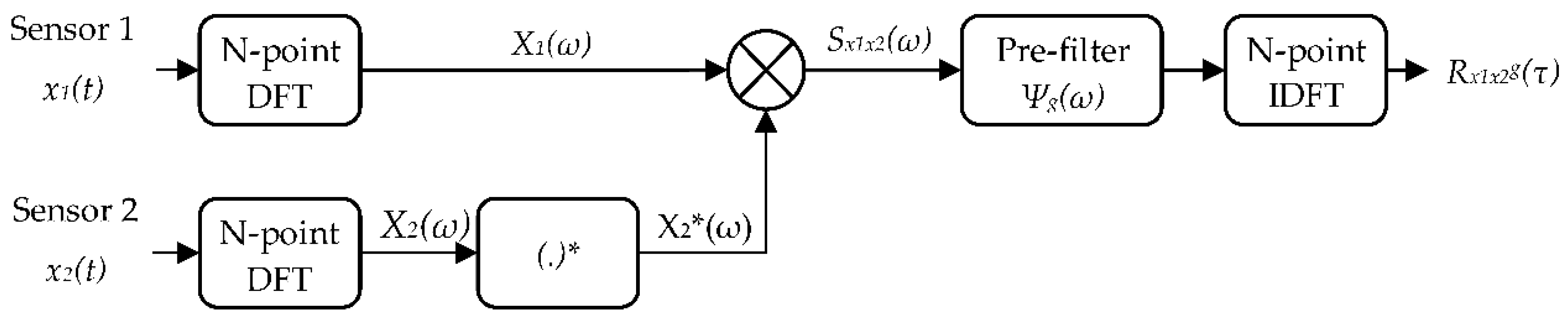
Figure 3.
Group speed dispersive curves of the flexural modes in the frequency band 0–400 kHz for the given gas pipe.
Figure 3.
Group speed dispersive curves of the flexural modes in the frequency band 0–400 kHz for the given gas pipe.

Figure 4.
The MLPNN with input, hidden, and output layers.
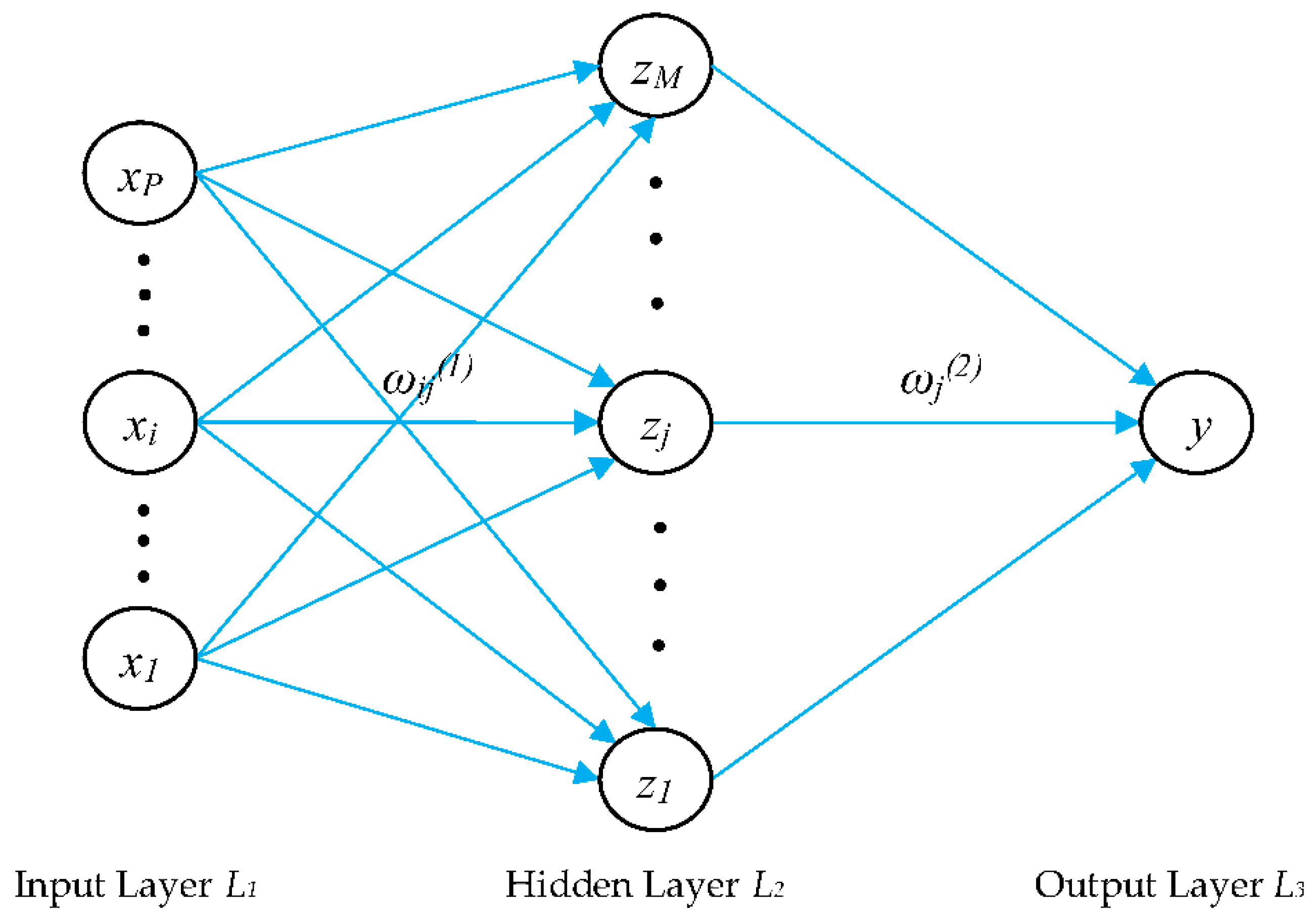
Figure 5.
Experiment system diagram: (i) a gas pipe, (ii) two AE sensors, (iii) an impulse hammer, (iv) a data acquisition card, (v) a PC, and (vi) a hose.
Figure 5.
Experiment system diagram: (i) a gas pipe, (ii) two AE sensors, (iii) an impulse hammer, (iv) a data acquisition card, (v) a PC, and (vi) a hose.

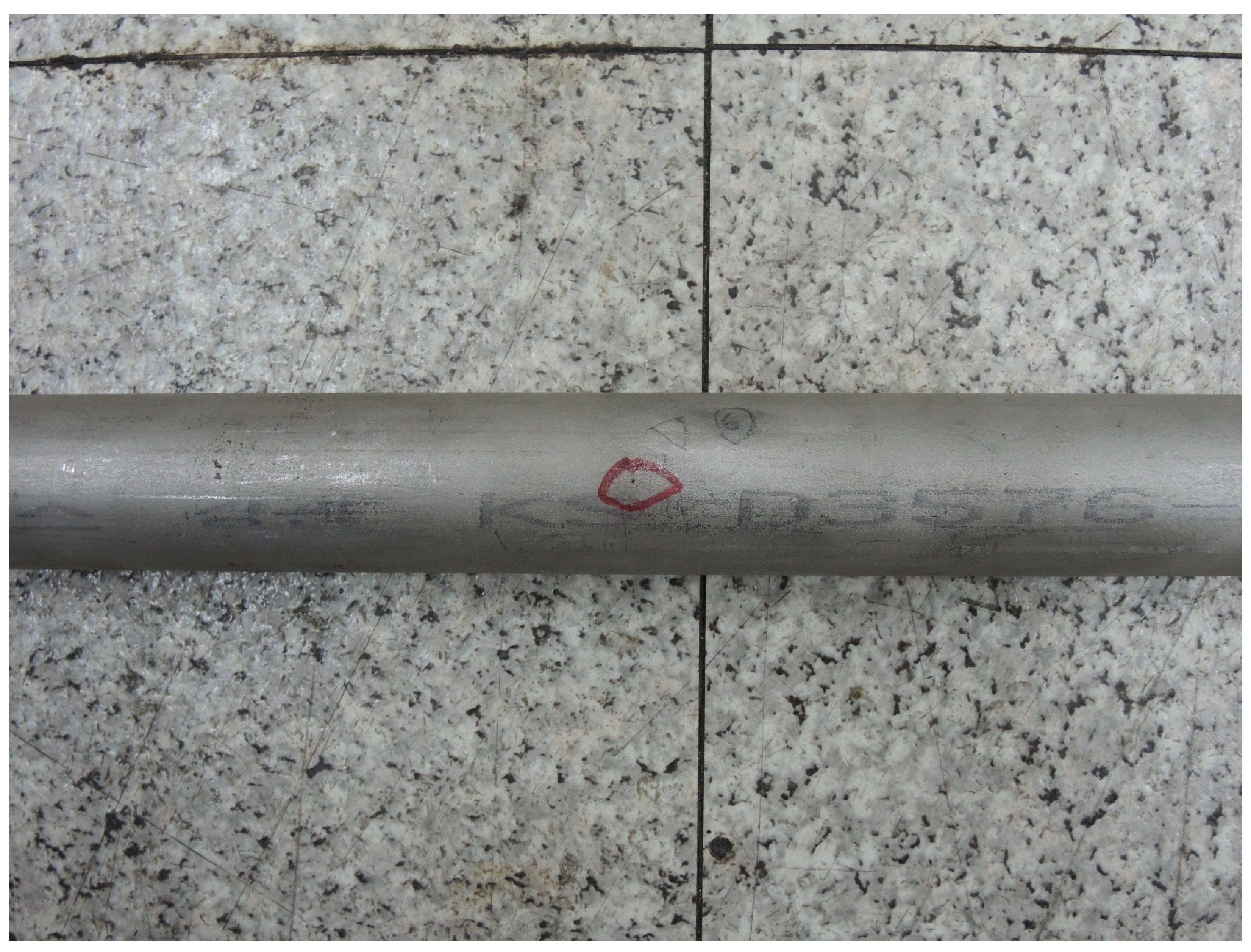
Figure 6.
A simulated leak orifice of the pipe.

Figure 7.
The AE sensor mounted with the magnetic hold down and vacuum grease couplant.
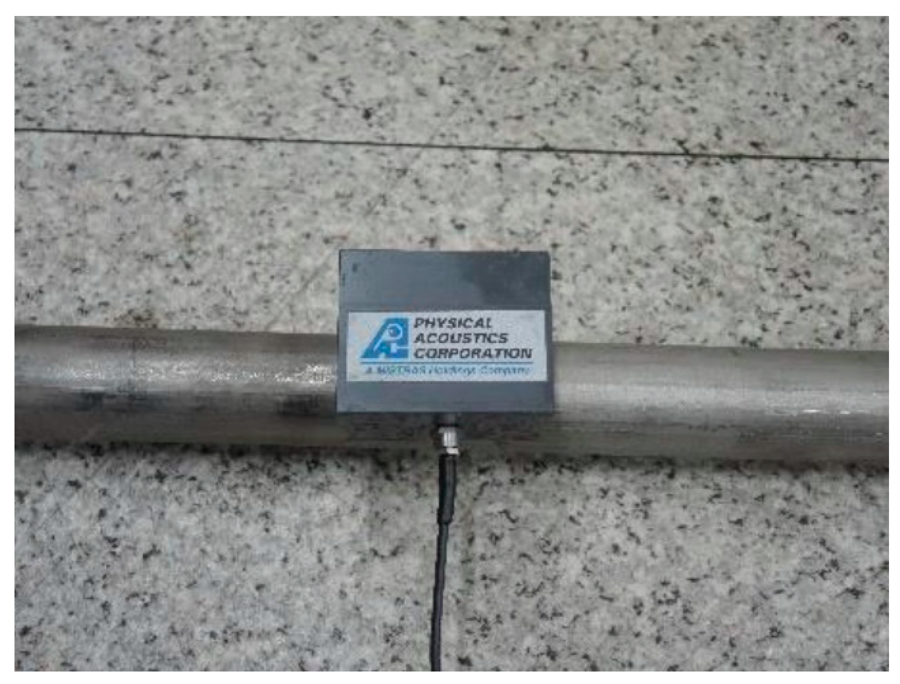
Figure 8.
An impulse hammer.
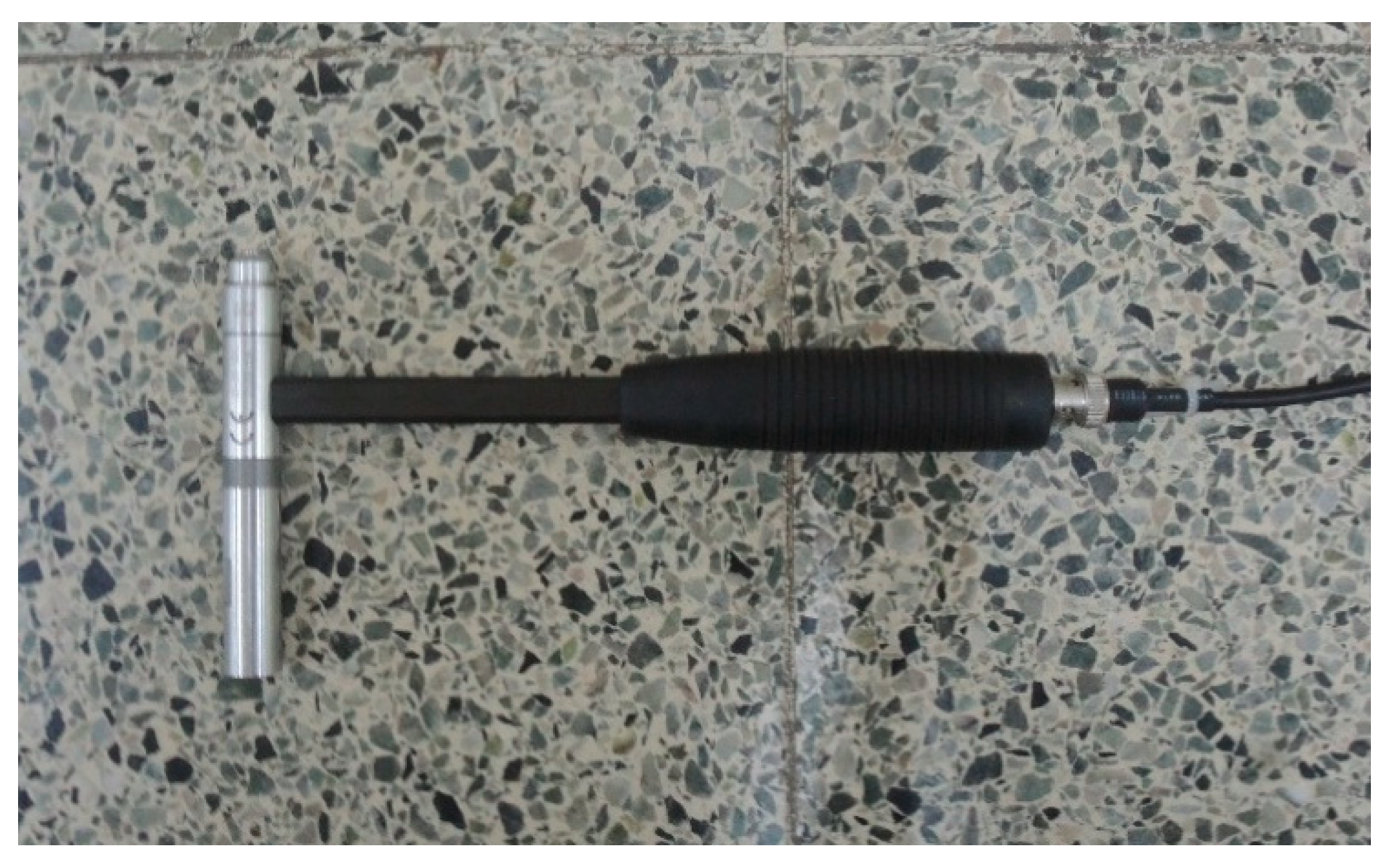
Figure 9.
The placement of two AE sensors along the pipe.
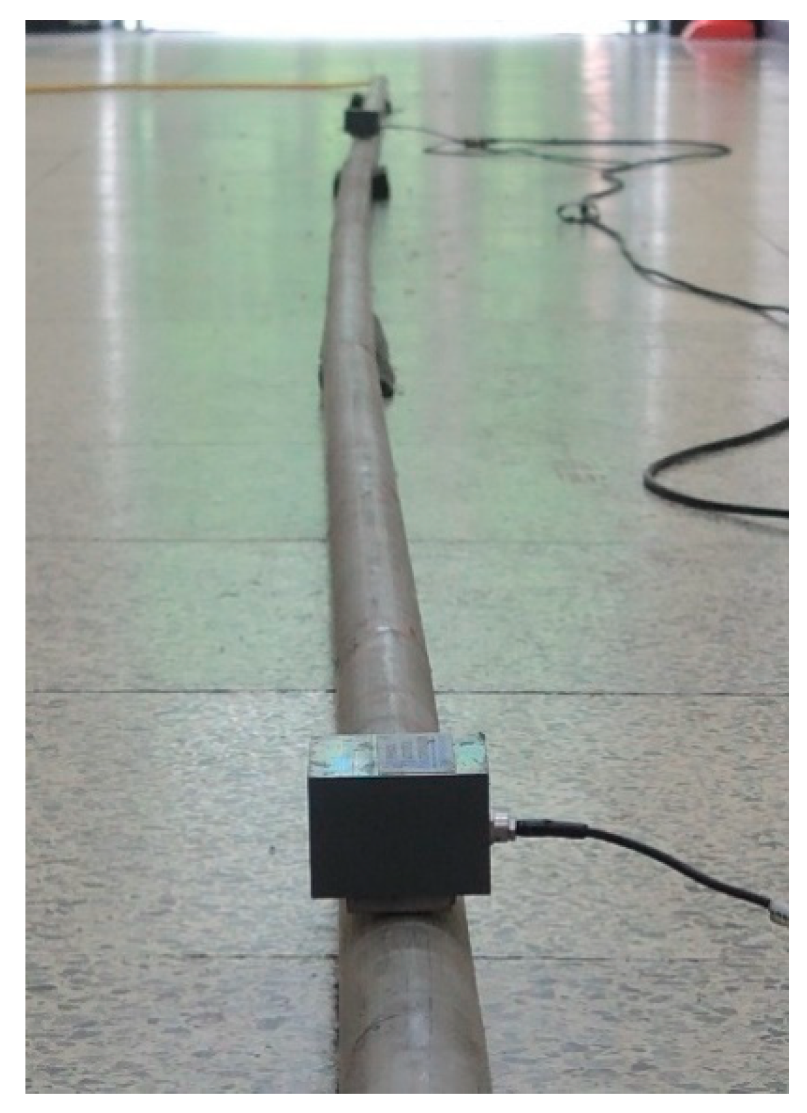
Figure 10.
Flowchart of the leakage location method for the MLPNN locator.
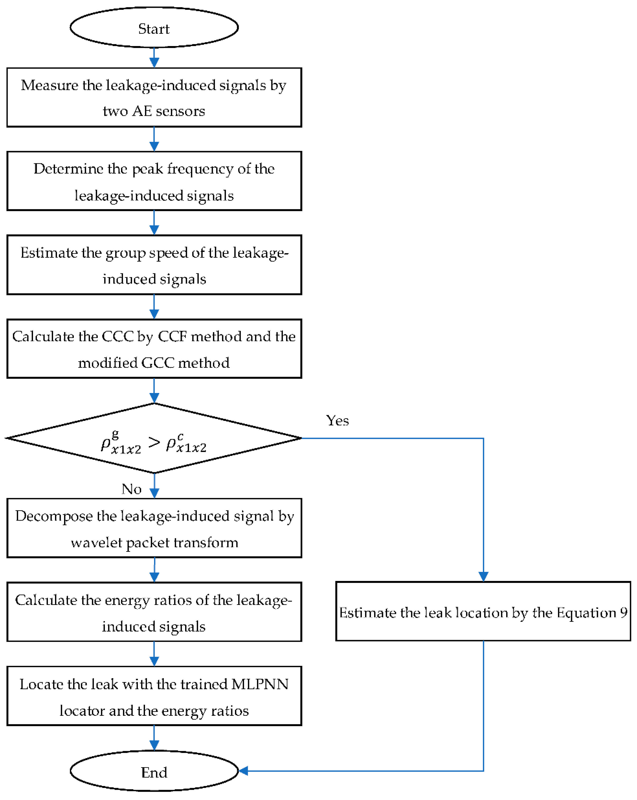
Figure 11.
Comparison of the power spectral densities of the leakage-induced signal in the different distances (L1 = 1 m, 2 m) away from the leak source.
Figure 11.
Comparison of the power spectral densities of the leakage-induced signal in the different distances (L1 = 1 m, 2 m) away from the leak source.
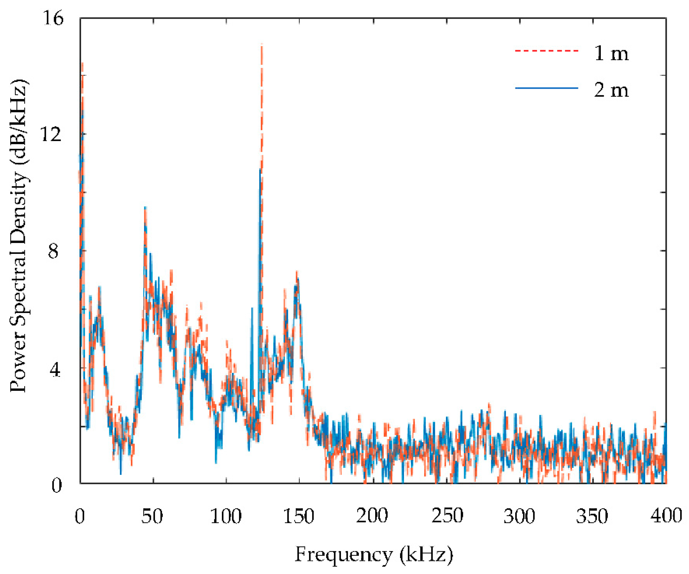
Figure 12.
Fitting curves of the signal energy ratios of the AE signals measured by the two sensors.
Figure 12.
Fitting curves of the signal energy ratios of the AE signals measured by the two sensors.

Figure 13.
Impulse response signals acquired at different distances from sensor 1: (a) 0.4m and (b) 13m.
Figure 13.
Impulse response signals acquired at different distances from sensor 1: (a) 0.4m and (b) 13m.

Figure 14.
Cross-correlation coefficients (CCCs) obtained by two methods: (a) CCF location method, and (b) modified GCC location method.
Figure 14.
Cross-correlation coefficients (CCCs) obtained by two methods: (a) CCF location method, and (b) modified GCC location method.
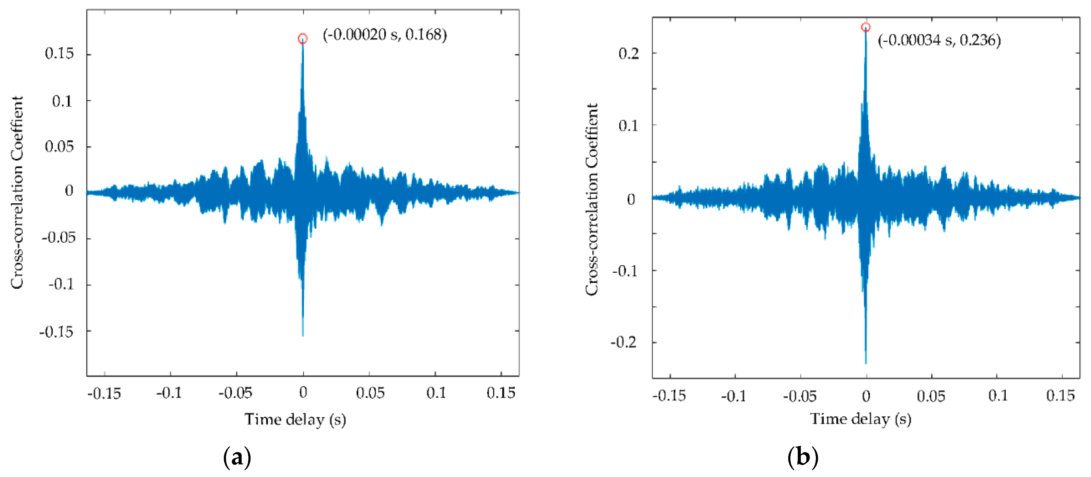
Figure 15.
Histograms of the relative location errors obtained by two methods: (a) CCF location method and (b) MLPNN locator.
Figure 15.
Histograms of the relative location errors obtained by two methods: (a) CCF location method and (b) MLPNN locator.

Table 1.
Material and geometric parameters of the given pipe.
| a (mm) | b (mm) | μ | ρ (kg/m3) | G (GPa) | E (GPa) |
|---|---|---|---|---|---|
| 13.9 | 16.7 | 0.35 | 8000 | 76 | 205 |
a is the inner radius of the pipe, b is the outer radius of the pipe, μ is the Poisson’s ratio of the pipe wall material, ρ is the density of the pipe wall material, G is the shear modulus of the pipe wall material, E is the Young’s modulus of the pipe wall material.
Table 2.
The location results obtained by the CCF location method.
| L (m) | 3.24 | 3.24 | 3.24 | 3.24 | 4.52 | 4.52 | 4.52 | 4.52 | 5.70 | 5.70 | 5.70 | 5.70 |
|---|---|---|---|---|---|---|---|---|---|---|---|---|
| f (kHz) | 124.2 | 123.8 | 123.4 | 125.4 | 105.5 | 103.4 | 107.2 | 106.7 | 104.7 | 104.3 | 104.7 | 103.5 |
| v (m/s) | 2404 | 2400 | 2397 | 2415 | 2200 | 2173 | 2222 | 2215 | 2190 | 2186 | 2190 | 2175 |
| l1 (m) | 2.16 | 2.16 | 2.16 | 2.16 | 2.16 | 2.16 | 2.16 | 2.16 | 2.16 | 2.16 | 2.16 | 2.16 |
| (m) | 1.78 | 1.71 | 1.82 | 1.72 | 1.70 | 1.77 | 1.75 | 1.79 | 1.83 | 1.74 | 1.79 | 1.83 |
| ∆l1 (m) | 0.38 | 0.45 | 0.34 | 0.44 | 0.46 | 0.39 | 0.41 | 0.37 | 0.33 | 0.42 | 0.37 | 0.33 |
| δl1 (%) | 17.6 | 20.1 | 15.7 | 20.4 | 21.3 | 18.1 | 19.0 | 17.1 | 15.3 | 19.4 | 17.1 | 15.3 |
L is the distance between the two AE sensors, f is the peak frequency of the leakage-induced signal, v is the group speed estimation of the leakage-induced signal, l1 is the real distance between the leak and sensor 1, is the distance estimation between the leak and sensor 1, ∆l1 is the leakage location error, δl1 is the relative location error.
Table 3.
The location results obtained by the MLPNN locator.
| L (m) | 3.24 | 3.24 | 3.24 | 3.24 | 4.52 | 4.52 | 4.52 | 4.52 | 5.70 | 5.70 | 5.70 | 5.70 |
|---|---|---|---|---|---|---|---|---|---|---|---|---|
| f (kHz) | 124.2 | 123.8 | 123.4 | 125.4 | 105.5 | 103.4 | 107.2 | 106.7 | 104.7 | 104.3 | 104.7 | 103.5 |
| v (m/s) | 2404 | 2400 | 2397 | 2415 | 2200 | 2173 | 2222 | 2215 | 2190 | 2186 | 2190 | 2175 |
| l1 (m) | 2.16 | 2.16 | 2.16 | 2.16 | 2.16 | 2.16 | 2.16 | 2.16 | 2.16 | 2.16 | 2.16 | 2.16 |
| (m) | 2.19 | 2.18 | 2.20 | 2.25 | 2.26 | 2.09 | 2.25 | 2.27 | 1.99 | 2.23 | 2.28 | 1.98 |
| ∆l1 (m) | 0.03 | 0.02 | 0.04 | 0.09 | 0.10 | 0.07 | 0.09 | 0.11 | 0.17 | 0.07 | 0.12 | 0.18 |
| δl1 (%) | 1.4 | 0.9 | 1.9 | 4.2 | 4.6 | 3.2 | 4.2 | 5.1 | 7.9 | 3.2 | 5.6 | 8.3 |
© 2019 by the authors. Licensee MDPI, Basel, Switzerland. This article is an open access article distributed under the terms and conditions of the Creative Commons Attribution (CC BY) license (http://creativecommons.org/licenses/by/4.0/).
Share and Cite
MDPI and ACS Style
Wu, Q.; Lee, C.-M. A Modified Leakage Localization Method Using Multilayer Perceptron Neural Networks in a Pressurized Gas Pipe. Appl. Sci. 2019, 9, 1954. https://doi.org/10.3390/app9091954
AMA Style
Wu Q, Lee C-M. A Modified Leakage Localization Method Using Multilayer Perceptron Neural Networks in a Pressurized Gas Pipe. Applied Sciences. 2019; 9(9):1954. https://doi.org/10.3390/app9091954
Chicago/Turabian StyleWu, Qi, and Chang-Myung Lee. 2019. "A Modified Leakage Localization Method Using Multilayer Perceptron Neural Networks in a Pressurized Gas Pipe" Applied Sciences 9, no. 9: 1954. https://doi.org/10.3390/app9091954
Note that from the first issue of 2016, this journal uses article numbers instead of page numbers. See further details here.