An Integrated Adaptive Kalman Filter for High-Speed UAVs


College of Biomedical Engineering & Instrument Science, Zhejiang University, Hangzhou 310007, China
*
Author to whom correspondence should be addressed.
†
These authors contributed equally to this work.
Appl. Sci. 2019, 9(9), 1916; https://doi.org/10.3390/app9091916
Submission received: 28 March 2019
/
Revised: 30 April 2019
/
Accepted: 2 May 2019
/
Published: 9 May 2019
(This article belongs to the Special Issue Unmanned Aerial Vehicles (UAVs))
Abstract
:In order to solve the problems of filtering divergence and low accuracy in Kalman filter (KF) applications in a high-speed unmanned aerial vehicle (UAV), this paper proposed a new method of integrated robust adaptive Kalman filter: strong adaptive Kalman filter (SAKF). The simulation of two high-dynamic conditions and a practical experiment were designed to verify the new multi-sensor data fusion algorithm. Then the performance of the Sage–Husa adaptive Kalman filter (SHAKF), strong tracking filter (STF), H∞ filter and SAKF were compared. The results of the simulation and practical experiments show that the SAKF can automatically select its filtering process under different conditions, according to an anomaly criterion. SAKF combines the advantages of SHAKF, H∞ filter and STF, and has the characteristics of high accuracy, robustness and good tracking skill. The research has proved that SAKF is more appropriate in high-speed UAV navigation than single filter algorithms.
1. Introduction
Due to their advantages of high-maneuverability and long flight range, high-speed unmanned aerial vehicles (UAVs) are widely used in scout, tracking, danger monitoring, etc. [1]. Compared with a low-speed UAV, a high-speed UAV is more easily interfered in by the working mode and condition, which means a high-speed UAV needs reliable navigation system to provide long-term and accurate navigation information in complex environments [2]. The single Strap-down Inertial Navigation System (SINS) or single Global Navigation Satellite System (GNSS) cannot provide precise guidance for a UAV, so a SINS/GNSS information fusion system is needed [3]. Thus, an integrated navigation system is proposed, which combines the advantage of both sides and avoids their deficiencies [4,5]. It has been widely acknowledged that Kalman filter (KF) can be used in SINS/GNSS information fusion [6,7]. Based on H2 estimation, KF needs suitable initial values, system noise covariance matrix (Q-matrix) and measurement noise covariance matrix (R-matrix) to reach the optimal estimation. Meantime, the hypothetical condition of KF is that the system model is accurate and the noise characteristic obeys or approximately obeys Gaussian distribution. However, in the flight process, a high-speed UAV usually faces a high-dynamic environment such as large maneuvering and wide spectrum vibration. Here, the large maneuvering means that the amplitude of linear acceleration or angular velocity is large and the frequency is low. Wide spectrum vibration refers to the condition that the vibration frequency range is wide, but the vibration amplitude is small [8]. Under the condition of a high-dynamic environment, the practical noise’s feature of the sensors is time-varying. The system model is also uncertain because GNSS may work in an abnormal state and the error of the inertial sensors may increase. So the filtering accuracy of KF will be seriously influenced by the uncertainty of system model and noise characteristic, and even worse, the filtering results may diverge. This will cause the UAV to be guided with a wrong route or even to crash [5]. If the value of Q-matrix or R-matrix is only adjusted blindly, the weight of real-time measurement and one-step prediction may be more appropriate to some extent, but it is impossible to achieve the optimal estimation. To solve the aforementioned problems of KF, changing the intermediate steps of KF is an effective way to improve the robustness and self-adaptive ability of the filtering algorithm. Aiming at adaptive estimation of Q-matrix and R-matrix, the Sage–Husa adaptive Kalman filter (SHAKF) was proposed [9,10,11]. Theoretically, this algorithm adaptively estimates the noise characteristic of system and measurement, and solves the uncertainty of KF for noise estimation. However, the noise covariance matrix is prone to losing the positive semi-definiteness and causes filtering divergence. The strong tracking filter (STF), trying to refine the priori estimate error covariance matrix (P-matrix), imports fading factor to reduce the influence of priori and historical information to current state estimation [12]. This method is good at tracking the abrupt changes. In reference [13], researchers used STF for sensor fault diagnosis in a UAV control system, and the simulation results showed good performance in real-time and accuracy. The reference [14,15] proposed an adaptive fuzzy strong tracking extended Kalman filter structure which combines STF and fuzzy logic model. This method was respectively used in pure Global Position System (GPS) navigation and Inertial Navigation System (INS)/GPS integrated navigation, which could improve the self-adaptive ability of system. But the measuring problem of a real vehicle in high-dynamic environment is not discussed.
In addition, robust filtering methods such as H∞ filter were also used in practical system [16,17,18]. The H∞ filter could minimize the influence of noise and initial state uncertainty, although Q-matrix, R-matrix and P0-matrix are unknown [19]. Its robustness can guarantee its availability, even in the worst case. The algorithm is suitable for all possible external interference, though it sacrifices average accuracy to maintain its stability [20].
In order to take the anti-interference ability and the accuracy of the filtering algorithm into account, this paper proposed an integrated filtering algorithm—strong adaptive Kalman filter (SAKF), based on SHAKF, STF and H∞ filter. The algorithm guarantees the stability and accuracy in high-dynamic flight of UAV, when the measurement noise is uncertain and the system’s interference is unavoidable because of the body vibration. SAKF adopts the method of SHAKF to realize adaptive estimation of noise covariance matrices. The R-matrix is considered as the criterion as to whether the filtering process is abnormal or not. Under normal condition, the STF is selected to provide high filtering accuracy. In abnormal situation, H∞ filter is used to guarantee the stability of filter.
The key innovation of this filtering algorithm is integration. In the process of our research we found that single filtering algorithm can hardly achieve the best performance in every aspect. So integrating the isolating algorithms is a feasible solution. Comparing with SHAKF, SAKF has a better tracking ability, which means it can closely track the abrupt change in high-dynamic flight. So SHAKF is better at adaptivity than SHAKF. Compared with STF, SAKF is more stable, which means such a method is not easy to diverge and can withstand unexpected interference; Compared with H∞ filter, SAKF has a higher accuracy, so this method can provide a better navigation. All of these advantages make the integrated filtering algorithms have good performance for high-dynamic navigation.
To verify the superiority of SAKF, simulations and practical experiments were designed to compare the performance of different filter algorithms. The results show that SAKF has greater advantages in anti-interference and accuracy, which is suitable for the integrated navigation of UAV in a high-dynamic environment.
2. Strong Adaptive Kalman Filter (SAKF)
2.1. Strap-down Inertial Navigation System/Global Navigation Satellite System (SINS/GNSS) Integrated Navigation State Model
For a high-speed UAV system, the state vector of navigation is defined as X, whose elements include INS error and inertial sensors’ error.
The navigation system is based on the East-North-Up (ENU) frame, and is the error components of attitude; represents the error components of velocity in the ENU frame; represents the error components of latitude, longitude and height; represents the drift of gyroscope in body frame; represents the bias of accelerometer in body frame. The superscripts b, n respectively represent body frame and ENU frame. T represents the transposition of the matrix.
The state equation is given as follows,
where represents the measurement noise of gyroscope and accelerometer; () represents the transition matrix; represents the noise exciting matrix.
SINS/GNSS integrated system uses loosely coupled closed-loop architecture, and the measurement equation is given as follows,
where represents measurement matrix; , and and represent the velocity and position’s measurement noise of satellite receiver; and respectively represent the velocity obtained by INS and GNSS; and respectively represent the position obtained by INS and GNSS.
2.2. Algorithm Designs
Under the condition that the system model and noise characteristic are already known, KF is linear optimal. The SHAKF breaks the constraint that Q-matrix and R-matrix must be known beforehand, and realizes the on-line estimation of system and measurement noise. This method puts more weights on the residual, and can improve the tracking ability in a high-dynamic environment. However, if practical measurement noise is lower than theoretical one or the priori estimation error is too large, R-matrix may lose its positive definiteness, so that the filtering results will diverge. By using fading factor when calculating P-matrix, STF reduces the weights of the prior knowledge and historical information in current state estimation. Therefore, this method is a good way to track sudden changes. The basic assumption of STF, like KF, is that the noise characteristic obeys or approximately obeys Gaussian distribution. However, the noise under the high-dynamic flight condition of UAV cannot be described as Gaussian distribution. For example, there may be hopping points in GNSS data, thus a large estimation error will occur by then. The H∞ filter can guarantee the system’s availability under the condition of strong interference, but its average accuracy decreases. The proposed method of integrated filtering, strong adaptive Kalman filter, combines the three methods mentioned above. Based on the framework of KF, SAKF adds adaptive estimation step for error covariance matrices, and R-matrix is considered as the criterion whether the filtering process is abnormal or not. In abnormal condition, the algorithm will choose H∞ filter as the filtering main body. Otherwise, STF will be chosen.
Figure 1 shows the process of SAKF. The whole process includes 4 parts.
Part 1. State prediction update equation is given as follows, is the priori state estimation at step k. is the estimation from time step k − 1 to k. relates the state at time step k to the state at step k + 1.
Part 2. Residual update equation is given as follows, is the residual at step k, is the measurement value at step k, and represent the measurement matrix.
Part 3. Measurement of anomaly detection step
The adaptive estimation method for the Q-matrix and R-matrix does not conflict with the framework of STF and H∞ filter, but the intermediate steps of STF and H∞ filter are conflicts with each other. So it is necessary to judge whether the measurement information is abnormal. The algorithm can use STF under normal condition, or switch to the H∞ filter under abnormal conditions.
Firstly, we should set the upper bound of R-matrix, and the matrix of maximum values named is given as follows,
where is the number of measurement vectors. Before each update, a detection should be made to check whether the estimated value of the vector in R-matrix is smaller than (). The inequality is given as follows, whose result is considered as the criterion of anomaly or divergence. Here, the superscript means this variable corresponding the vector in R-matrix.
When every satisfies the condition of inequality (7), we believe the measurement results are usable and the filter’s work state is stable. So the R-matrix update equation can be showed as follows,
Then update the measurement information using the updated equation of STF, which is given as follows:
Here represents the diagonal matrix of fading factors, which is given as follows,
Each fading factor can be gotten by Equation (11).
where is a fixed parameter, and the value of can be obtained by Equations (12)–(16).
where the initial value of is set as the covariance matrix of residual. Then the forgetting factor adjusts the ratio between and in the following iterations. As , . This indicates that a lager weight is put on the current information than historical information. Therefore, the residual plays an important role in the filtering process, and the tracking ability can be improved in this way.
If there exists which does not satisfy , then the elements of R-matrix are updated as follows,
Then the updated equation of H∞ filter is used as the filtering step:
Set constrain condition for iteration, like Equation (19),
As is a key parameter for filtering performance, it is difficult to select an appropriate value. Generally, when the Equation (19) is satisfied, should be maximized to achieve the highest robustness. However, the UAV navigation system is time-varying, the Equation (19) may not satisfy with a large . Thus, when in high-dynamic environment, the value of is set to be relatively smaller. is usually set at the range of in navigation. Here, represents error covariance matrix of ’s linear combination. Usually, is set to be equal to (unit matrix) in navigation.
Part 4. The Q matrix update equation is given as follows
where and respectively represent adjusting factors of Q-matrix and R-matrix. Essentially, they relate to the ratio between residual and historical information. The estimation’s adaptive and tracking skills rely more on current information. Therefore, we import forgetting factors and to reinforce the role of the residual. The recurrent equation is given as follows:
where , and . When the value of is large enough, there are and . Generally, the value of is between 0.9 and 0.999.
3. Verification and Analysis
The simulation data and the real measurement data were respectively used to verify the strong adaptive filtering algorithm proposed in this paper. In Section 3.1, the simulation was used for the verification. In Section 3.2, four kinds of algorithms were used on a real UAV testing platform. By comparing the performance of each algorithm, the superiority of SAKF was verified.
3.1. Performance Analysis of High-Speed Unmanned Aerial Vehicle (UAV) Integrated Navigation Algorithms Based on Simulation
3.1.1. Trajectory Simulation and Error Model
The ideal flight simulation data was generated by the trajectory generator, which corresponded to the high maneuvering condition (acceleration of 4~100 g; angular velocity of 100~1000°/h). The whole process includes take-off at an acceleration of 50 m/s2, climb at a pitch angular velocity of 35°/s, turning at a yaw angular velocity of 15°/s, descend at a pitch angular velocity of 30°/s, level flight, etc. The navigation frame is chosen as the E-N-U geography frame. The initial position is selected as 120° E, 30° N, and at an altitude of 1000 m. The simulation process lasts 450 s, and the configuration of sensors and initial errors information are showed in Table 1.
Figure 2 shows the diagram of trajectory generated by simulation system.
In addition, the sampling frequency of inertial sensors is 200 Hz, the update rate of SINS is 100 Hz, and the update rate of GNSS is 1 Hz. The filtering parameters are showed as follows, , , , , , . Here, represents semimajor axis of ellipsoid.
3.1.2. Scene Design
In order to verify the performance of the proposed strong adaptive filtering method, it is necessary to simulate the high-dynamic environment of the UAV. So we designed two kinds of scenes that are representative.
- Scene 1. Anomaly of SINS is simulated. During 250 s to 300 s, the drift of gyroscope is set at 20°/h, and the random walk is set at ; The bias of accelerometer is set at 40 mg, and the random walk is set at .
- Scene 2. Anomaly of GNSS is simulated. During 100 s to 150 s, the error of horizontal position is set at 40 m, and the vertical one is 50 m; the error of horizontal velocity is set at 0.5 m/s, and the vertical one is 2 m/s. The hopping point appears during 230 s to 232 s, where latitude data steps with 0.008°.
The accuracy and anti-interference ability of SHAKF, H∞ filter, STF and SAKF is compared by calculating the root-mean-square (RMS) of the filtering output.
Here, represents the ith true value of navigation, represents the Ith filtering results, and represents the times of filtering iteration.
3.1.3. Results and Analysis of Simulation
According to the simulation, the diagrams of errors (position, velocity and attitude) obtained by four types of filtering algorithms in scene 1 are given as Figure 3; Figure 4 shows the errors in scene 2.
To make a more accurate comparison, the RMS of four algorithms in two scenes is listed in Table 2 and Table 3.
According to the results shown in the tables and diagrams above, in scene 1, no filtering divergence appears, but the attitude error increases in each case. The filtering error obtained by SHAKF increases rapidly during 250 s~300 s, but the filtering results converge after this period; the anti-interference performance of H∞ filter and STF is better, as there is no apparent fluctuation in error during 250 s~300 s. However, the error obtained by H∞ filter is larger, especially the error of position after 300 s, where a severe fluctuation appears; by contrast, SAKF performs in a stable state during the whole simulation period, and its accuracy is higher than STF. For attitude, we noticed that the error of yaw is always in a relatively high level. There are two reasons to explain such situation. On one hand, the system did not use the information provided by GNSS to fix the yaw angle. On the other hand, because of the filtering constraint, the error of attitude was always at a controllable range without divergence. During 250 s~300 s the anomaly of inertial sensors occurs, which influences the accuracy of calculated yaw. As H∞ is relatively insensitive to abrupt change, it seems that the error of yaw is lower than STF and SAKF.
In scene 2, we lowered the accuracy of GNSS during 100~150 s and set a hopping point during the period of 230~232 s. Based on barometer and inertial sensors, we used the complementary filter to calculate the vertical position and velocity, so they were hardly influenced by anomalies of GNSS during the period of 100~150 s; At the same time, the horizontal estimation accuracy of STF and SHAKF deteriorate rapidly into the H∞ filter level; SAKF has the best performance in this period. During 230 s~232 s, SHAKF and STF are sensitive to the hopping point. STF is more easily influenced by hopping point than SHAKF but it also converges faster after the anomaly. On the other hand, the H∞ filter is insensitive to this situation. Since SAKF shares similar robustness with H∞ filter, it is hardly influenced by the hopping point. In summary, the SHAKF has the best accuracy without interference, but its accuracy is rapidly reduced when interference is introduced, even filter divergence may occur. The STF relies more on the measurement information, which is insensitive to the inertial anomaly. However it is easily influenced by the anomaly of GNSS. H∞ filter guarantees the stability in interference and shows high robustness when facing an anomaly, whereas its performance is limited by low-accuracy. The proposed algorithm, SAKF, which combines the advantages of three filtering methods, well fits for the high-dynamic flight of the UAV.
3.2. Practical Data Based Verification
3.2.1. Experimental Environment
In order to make it more convenient to compare the performance of four filtering algorithms, we first need to obtain the real-time data of sensors in the flight process of the UAV. Then the application of the algorithm is carried out in the post-processing. The experimental data was collected by a self-developed integrated system on UAV. The system consists of a digital processing board, a GNSS receiver (OEM615), an inertial measurement unit (ADIS16488) and other sensors. The core components of the digital processing board are a digital signal processor (DSP) (SM320C6748-HIREL) and field-programmable gate array (FPGA) (XC5VLX30T), where they are connected by an external memory interface (EMIF). In order to ensure the parallel acquisition of sensor data, OEM615 and ADIS16488 are connected to the FPGA through their respective serial interface, and a RS-422 driver is connected to the FPGA as the external communication port of the system. Meantime, the FPGA also connects other digital sensors such as barometers, thermometers and so on. UART and RS-422 were chosen as the communicational protocol, and measurement data were saved in an SD card. Then we undertook the verification using MATLAB after the data were exported to the computer.
3.2.2. Flight Route Design
Assisted with remote-control, the UAV moved according to a pre-set flight route and collected data at the same time. The initial position of the experiment was at 100.464452° E, 41.021293° N, with an altitude at 980 m, and the yaw angle was 350° (the defined range of yaw angle is 0~360°; the true north is defined as 0°; the clockwise direction is positive). The whole process included,
- Take off at an acceleration of 40 m/s2 with a 12° pitch angle, until the UAV reaches an altitude of 1500 m;
- Turn right at an roll angle of 30° until the yaw angle reaches 75°;
- Move forward at an acceleration of 5 m/s2, in the meantime, climb to an altitude of 3500 m with a 12° pitch angle, then execute a 450 s-long level flight;
- Turn right at an roll angle of 30° until the yaw angle reaches 90°;
- Accelerate to 200 m/s, climb to an altitude of 6400 m with a 10° pitch angle, then execute a 450 s-long level flight;
- Turn right at an roll angle of 30° until the yaw angle reaches 270°, then execute a 350 s-long level flight;
- Turn right at an roll angle of 35° until the yaw angle reaches 90°, then execute a 300 s-long level flight;
- Turn right at an roll angle of 35° until the yaw angle reaches 270°;
- Descend to an altitude of 1500 m with a −10° pitch angle;
- Return to the initial position.
3.2.3. Hyper-Parameter and Initial Error
The update rate of inertial sensor’s data was 200 Hz. The update rate of GNSS was 25 Hz. The update rate of SINS was 150 Hz. The initial error of UAV is given in Table 4.
The filtering parameters are showed as follows, , , , , , . Because the real condition was slightly different from the simulated one, we changed the value of filtering parameters to reach the best performance.
3.2.4. Results and Analysis of Experiment
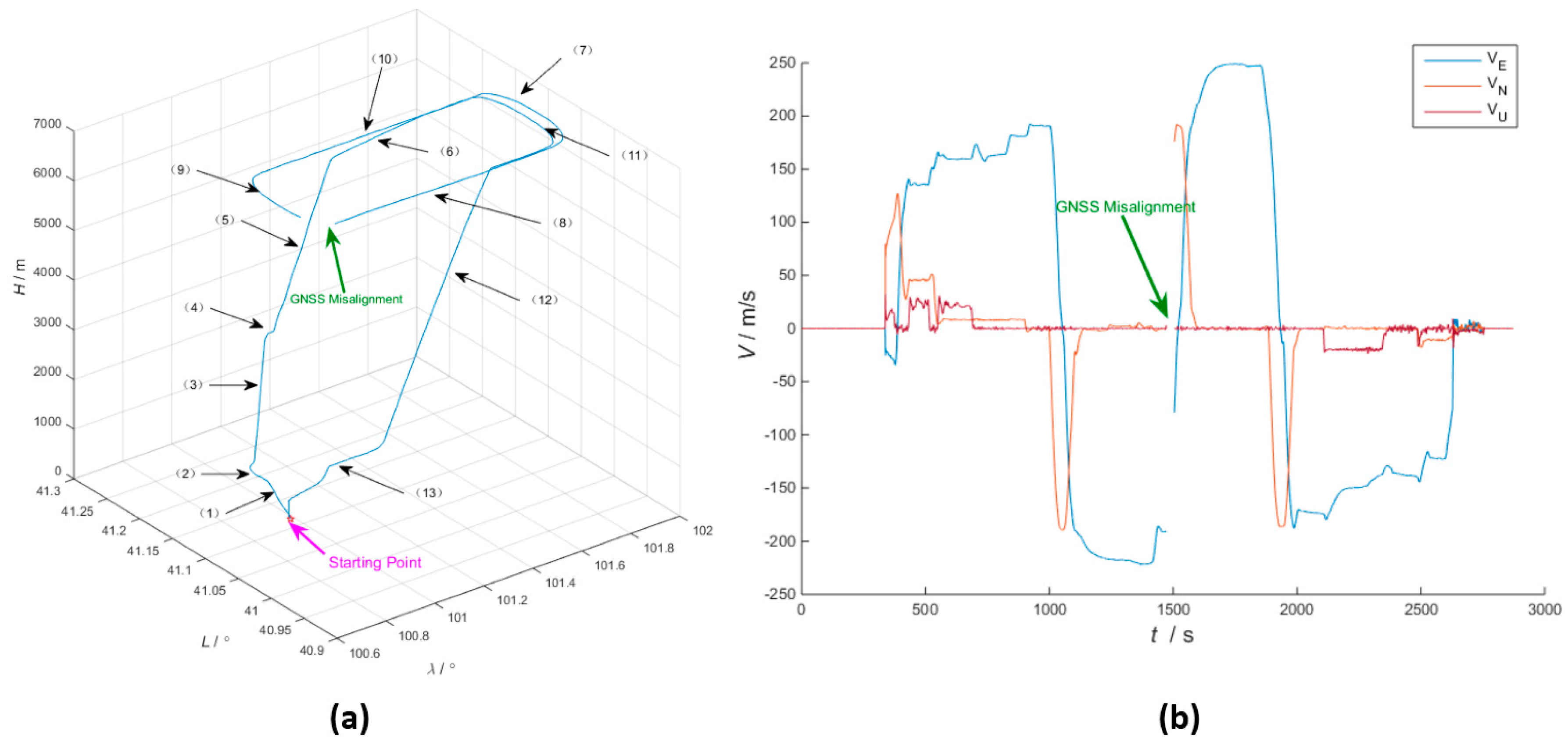
The whole process lasted 2873 s including take-off, flying and landing. Based on GNSS data, the diagrams of 3D trajectory and velocity curve in E-N-U frame are shown in Figure 5.
The red point in the 3D trajectory diagram is the starting point, and the sections marked with (1)~(13) correspond to the flight in Section 3.2.2. The label “GNSS Misalignment” in the diagram of the curve represents the anomaly of GNSS during 1470 s~1505 s (lock-loss, the number of satellite is less than 4). So GNSS information is not used for measurement update in this period.
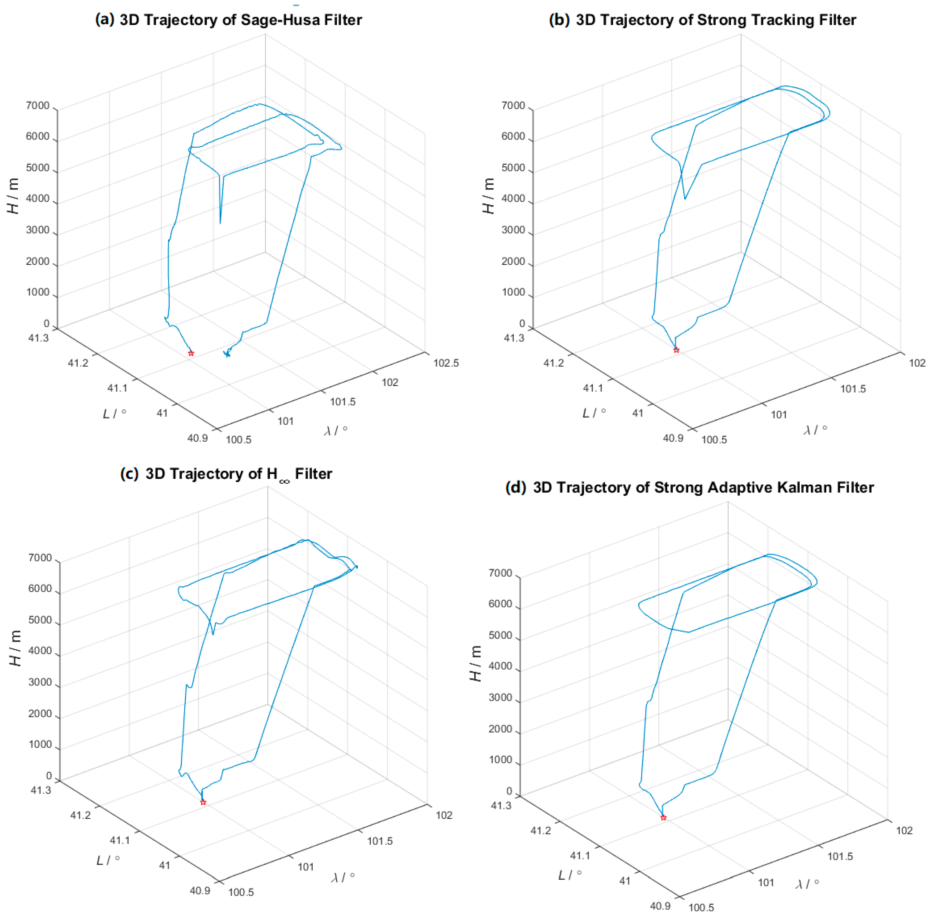
Comparing the performance of SHAKF, H∞ filter, STF and SAKF, the results are shown in Figure 6.
We choose some representative moments and use GNSS data as the reference, in order to compare the filtering accuracy of H∞ filter, STF and SAKF (divergence appears using SHAKF). The comparison is showed in Table 5.
Table 5 shows the accuracy comparison of the H∞ filter, STF and SAKF (divergence appears using SHAKF).
In Figure 6, the SHAKF method shows the filtering divergence, so it is not fitful in real high-dynamic environment. STF, whose accuracy closely depends on measurement information, has better tracking ability, but its accuracy will deteriorate when GNSS misalignment happens. The H∞ filter has great availability, even in the worst case, but its average accuracy is poor. SAKF has the best performance in the experiment. It maintains high stability and accuracy even when an anomaly appears. It can be seen from Table 5 that the error varies with time. The value of error in high-dynamic flight (500, 800, and 1800 s) is much larger than that in level flight (1000, 2500 s). Evaluating the accuracy of different filtering algorithms, SAKF is much better than STK and H∞ filter.
In summary, the proposed SAKF algorithm, which combines the advantages of SHAKF, STF and H∞ filter, fits the high-dynamic flight of a UAV well.
4. Conclusions
In this paper, an integrated adaptive filtering algorithm named SAKF is proposed, and the effectiveness of the algorithm is verified by simulation and a practical experiment, respectively. The results of the simulation and experiment showed that the SAKF has a better performance than other three algorithms in high-speed UAV integrated navigation system. It has the superiority of adapting to different disturbances during high-dynamic flight, and estimating measurement noise and system noise in real time. Meanwhile, it has the advantages of high accuracy, tracking ability and robustness. The proposed algorithm provides a new solution for a high-speed UAV navigation system.
At present, most of the data-fusion algorithms for an integrated navigation system in high-dynamic environment are still immature. Their verification is mostly based on pure simulation. We designed a real hardware testing platform, and used the real navigation data to verify its performance. We have proven the value of the proposed algorithm in the practical application in a high-speed UAV. In future, we will focus more on the real time and online navigation for UAV in high-dynamic conditions using SAKF. The further research of this new adaptive Kalman filtering algorithm will promote the development of high-speed UAVs and other fields of navigation.
Author Contributions
Conceptualization, T.H. and H.J.; Methodology, T.H. and H.J.; Software, H.J.; Validation, H.J. and Z.Z.; Formal Analysis, Z.Z.; Writing—Original Draft Preparation, H.J. and Z.Z.; Writing—Review and Editing, T.H. and Z.Z.; Project Administration, T.H. and L.Y.; Supervision, K.S.
Funding
This research was funded by China Aerospace Science and Technology Foundation, grant number 2018-HT-ZD-06.
Conflicts of Interest
The authors declare no conflict of interest.
Abbreviations
The following abbreviations are used in this manuscript:
| KF | Kalman filter |
| UAV | Unmanned Aerial Vehicle |
| SAKF | Strong Adaptive Kalman filter |
| SHAKF | Sage-Husa Adaptive Kalman filter |
| STF | Strong Tracking filter |
| SINS | Strap-down Inertial Navigation System |
| GNSS | Global Navigation Satellite System |
| GPS | Global Position System |
| INS | Inertial Navigation System |
| ENU | East-North-Up |
| DSP | Digital Signal Processor |
| FPGA | Field-Programmable Gate Array |
| EMIF | External Memory Interface |
References
- Mellinger, D.; Michael, N.; Kumar, V. Trajectory generation and control for precise aggressive maneuvers with quadrotors. Exp. Robot. 2014, 79, 361–373. [Google Scholar]
- Barry, A.J.; Tedrake, R. Pushbroom stereo for high-speed navigation in cluttered environments. In Proceedings of the IEEE International Conference on Robotics and Automation 2015, Seattle, WA, USA, 26–30 May 2015. [Google Scholar]
- Zhang, C.; Guo, C.; Zhang, D. Data fusion based on adaptive interacting multiple model for GPS/INS integrated navigation system. Appl. Sci. 2018, 8, 1682. [Google Scholar] [CrossRef]
- Liu, X.; Guo, X.; Zhao, D.; Shen, C.; Wang, C.; Li, J.; Tang, J.; Liu, J. INS/Vision integrated navigation system based on a navigation cell model of the hippocampus. Appl. Sci. 2019, 9, 234. [Google Scholar] [CrossRef]
- Rong, W.; Zhi, X.; Liu, J.Y.; Li, R.; Hui, P. SINS/GPS/CNS information fusion system based on improved Huber filter with classified adaptive factors for high-speed UAVs. In Proceedings of the Position Location & Navigation Symposium, Myrtle Beach, SC, USA, 23–26 April 2012; pp. 441–446. [Google Scholar]
- Jian-Wen, L.I.; Hao, S.Y. On precise positioning method for highly dynamic GPS/SINS integrated navigation. Inf. Control 2009, 38, 303–304. [Google Scholar]
- Zhang, B.; Wen, X.U.; Jianlong, L.I. Particle filter-based AUV integrated navigation methods. Robot 2012, 34, 80–85. [Google Scholar] [CrossRef]
- Min, S.; Wenqi, W.; Xianfei, P. Research on Error Analysis and Optimization Methods for Strapdown Inertial Navigation Algorithm under Highly Dynamic Environment; National Defense Industry Press: Beijing, China, 2017. [Google Scholar]
- Sage, A.P.; Husa, G.W. Algorithms for sequential adaptive estimation of prior statistics. In Proceedings of the Adaptive Processes, University Park, PA, USA, 17–19 November 1969. [Google Scholar]
- Shi, E. An improved real-time adaptive Kalman filter for low-cost integrated GPS/INS navigation. In Proceedings of the International Conference on Measurement, Harbin, China, 18–20 May 2012. [Google Scholar]
- Hajiyev, C.; Soken, E.H. Robust adaptive kalman filter for estimation of UAV dynamics in the presence of sensor/actuator faults. Dialogues Cardiovasc. Med. DCM 2013, 28, 376–383. [Google Scholar] [CrossRef]
- Zhou, D.H.; Frank, P.M. Strong tracking filtering of nonlinear time-varying stochastic systems with coloured noise: Application to parameter estimation and empirical robustness analysis. Int. J. Control 1996, 65, 295–307. [Google Scholar] [CrossRef]
- Tian, F.; Zheng, J.Y.; Zhang, T. Sensor fault diagnosis for an UAV control system based on a strong tracking kalman filter. Appl. Mech. Mater. 2014, 687, 270–274. [Google Scholar] [CrossRef]
- Jwo, D.J.; Wang, S.H. Adaptive fuzzy strong tracking extended kalman filtering for GPS navigation. Sensors 2007, 7, 778–789. [Google Scholar] [CrossRef]
- Jwo, D.J.; Huang, C.M. An adaptive fuzzy strong tracking Kalman filter for GPS/INS navigation. In Proceedings of the Conference of the IEEE Industrial Electronics Society, Taipei, Taiwan, 5–8 November 2007. [Google Scholar]
- Shaked, U. Minimum error state estimation of linear stationary processes. Autom. Control Trans. 1990, 35, 554–558. [Google Scholar] [CrossRef]
- Shaked, U.; Theodor, Y. H/sub infinity/-optimal estimation: A tutorial. In Proceedings of the IEEE Conference on Decision & Control, Tucson, AZ, USA, 16–18 December 2002. [Google Scholar]
- Hassibi, B.; Sayed, A.H.; Kailath, T. Linear estimation in Krein spaces—Part II: Applications. Autom. Control Trans. 1993, 41, 34–49. [Google Scholar] [CrossRef]
- Li, Z.; Chang, G.; Gao, J.; Jian, W.; Hernandez, A. GPS/UWB/MEMS-IMU tightly coupled navigation with improved robust Kalman filter. Adv. Space Res. 2016, 58, 2424–2434. [Google Scholar] [CrossRef]
- Hu, D.; Li, J.; Jin, H. Application of robust kalman filtering to integrated navigation based on inertial navigation system and dead reckoning. In Proceedings of the International Conference on Artificial Intelligence & Computational Intelligence, Sanya, China, 23–24 October 2010. [Google Scholar]
Figure 1.
The process of the strong adaptive Kalman filter. The whole flow chart includes state prediction, residual, and measurement anomaly detection, filtering of the main body, and Q Adaption.
Figure 1.
The process of the strong adaptive Kalman filter. The whole flow chart includes state prediction, residual, and measurement anomaly detection, filtering of the main body, and Q Adaption.
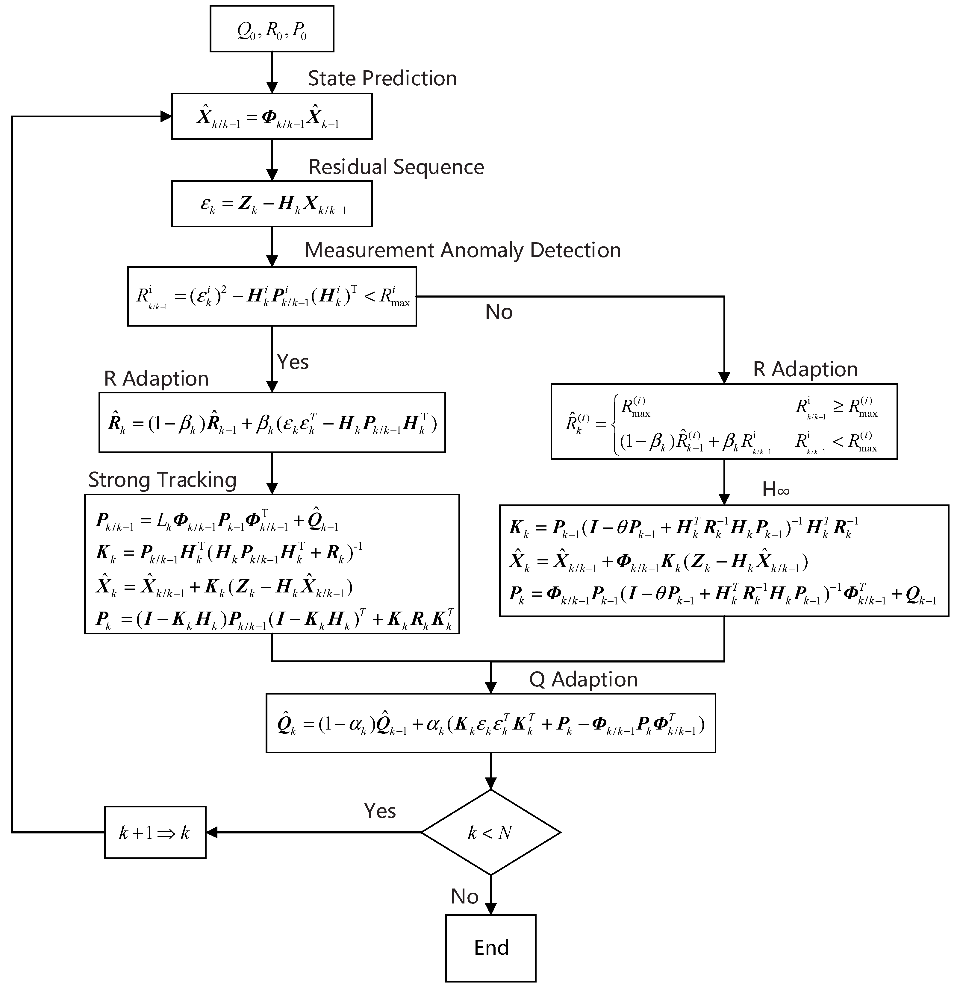
Figure 2.
Diagram of simulated position, velocity and attitude (truth value).
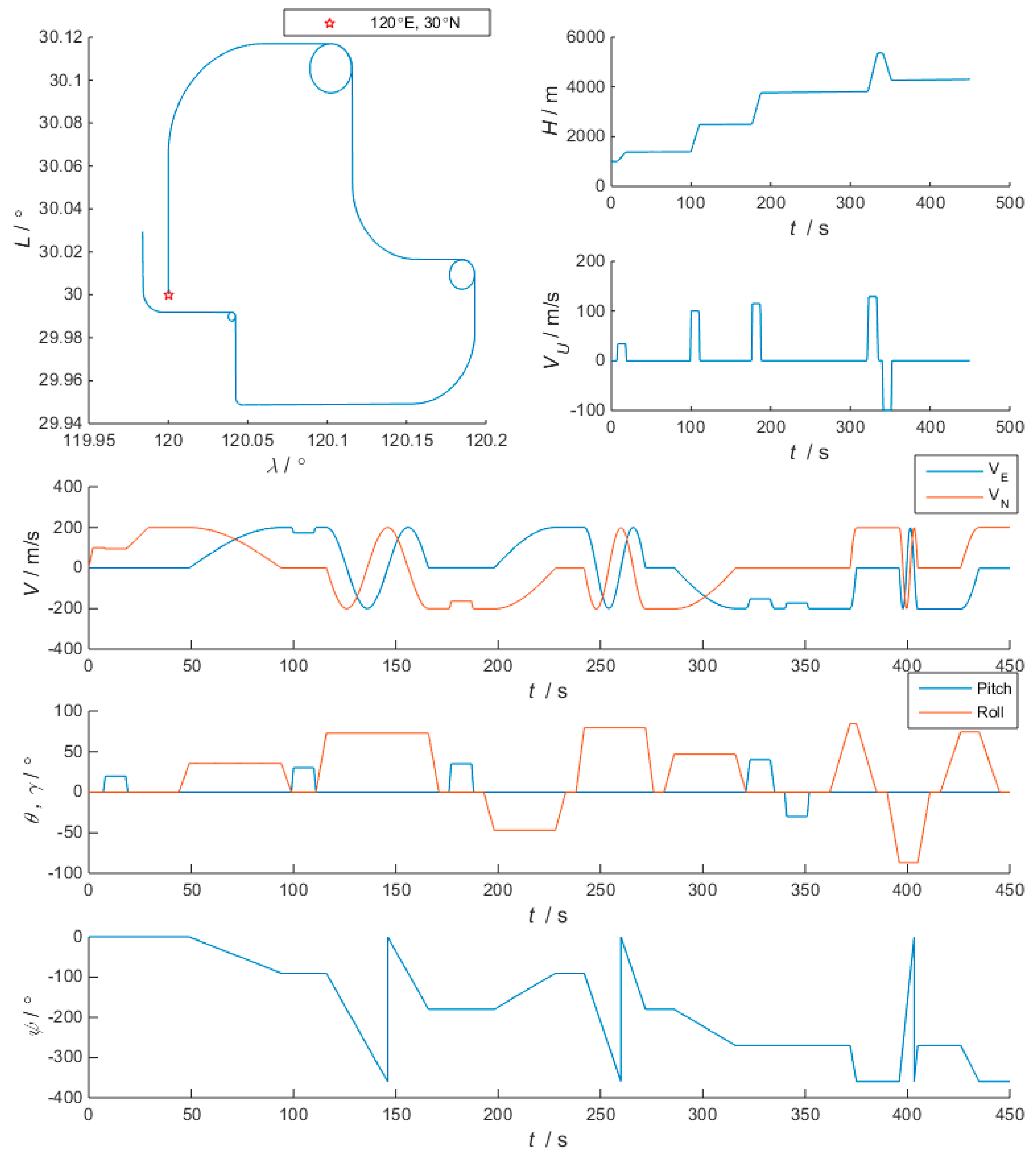
Figure 3.
The diagrams of errors obtained by four types of filtering algorithms in scene 1 designed in 3.1.2. (a) Sage–Husa adaptive Kalman filter (SHAKF); (b) strong tracking filter (STF); (c) H∞ filter; (d) strong adaptive Kalman filter (SAKF).
Figure 3.
The diagrams of errors obtained by four types of filtering algorithms in scene 1 designed in 3.1.2. (a) Sage–Husa adaptive Kalman filter (SHAKF); (b) strong tracking filter (STF); (c) H∞ filter; (d) strong adaptive Kalman filter (SAKF).
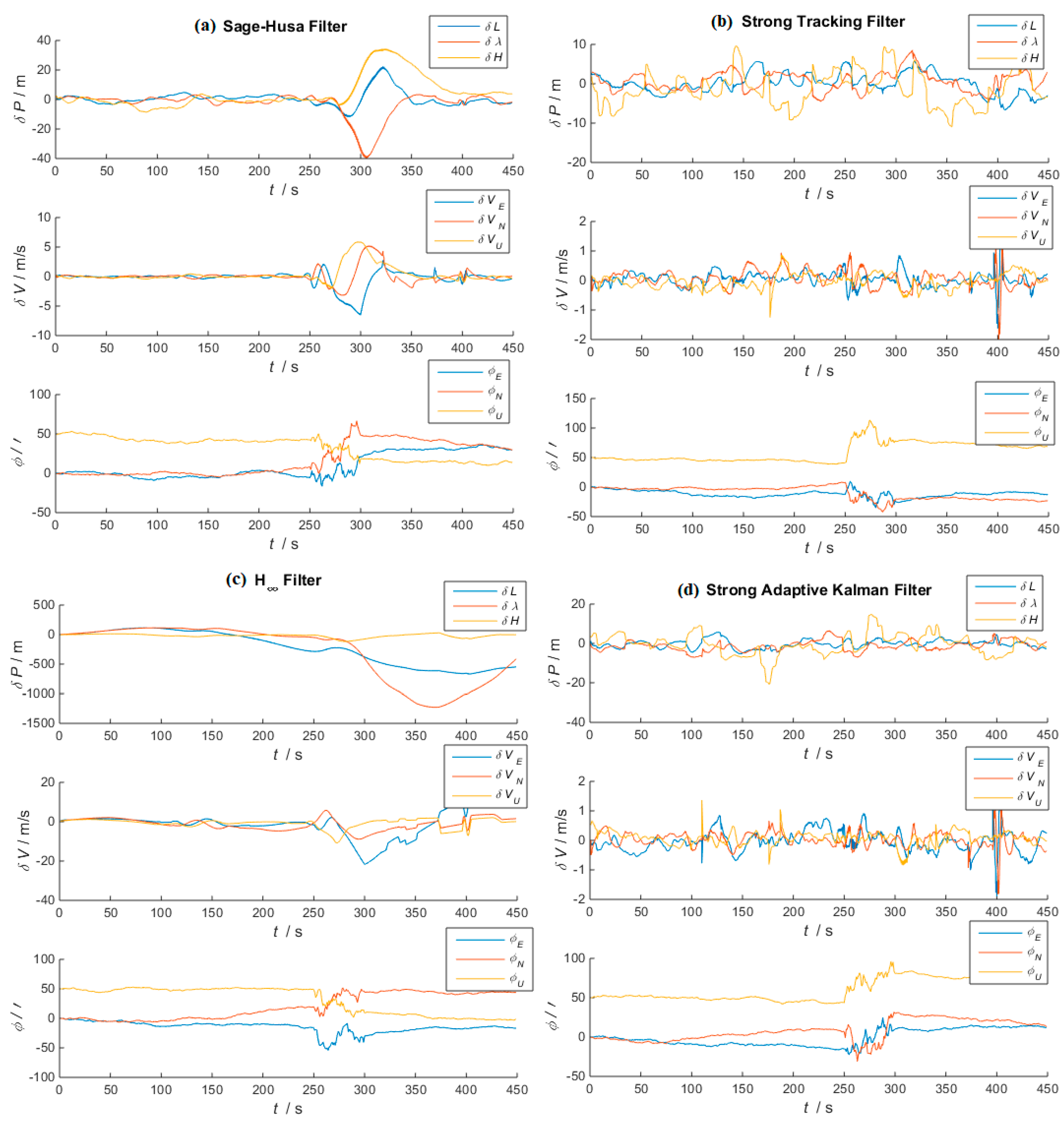
Figure 4.
The diagrams of errors obtained by four types of filtering algorithms in the scene 2 designed in 3.1.2. (a) SHAKF; (b) STF; (c) H∞ filter; (d) SAKF.
Figure 4.
The diagrams of errors obtained by four types of filtering algorithms in the scene 2 designed in 3.1.2. (a) SHAKF; (b) STF; (c) H∞ filter; (d) SAKF.
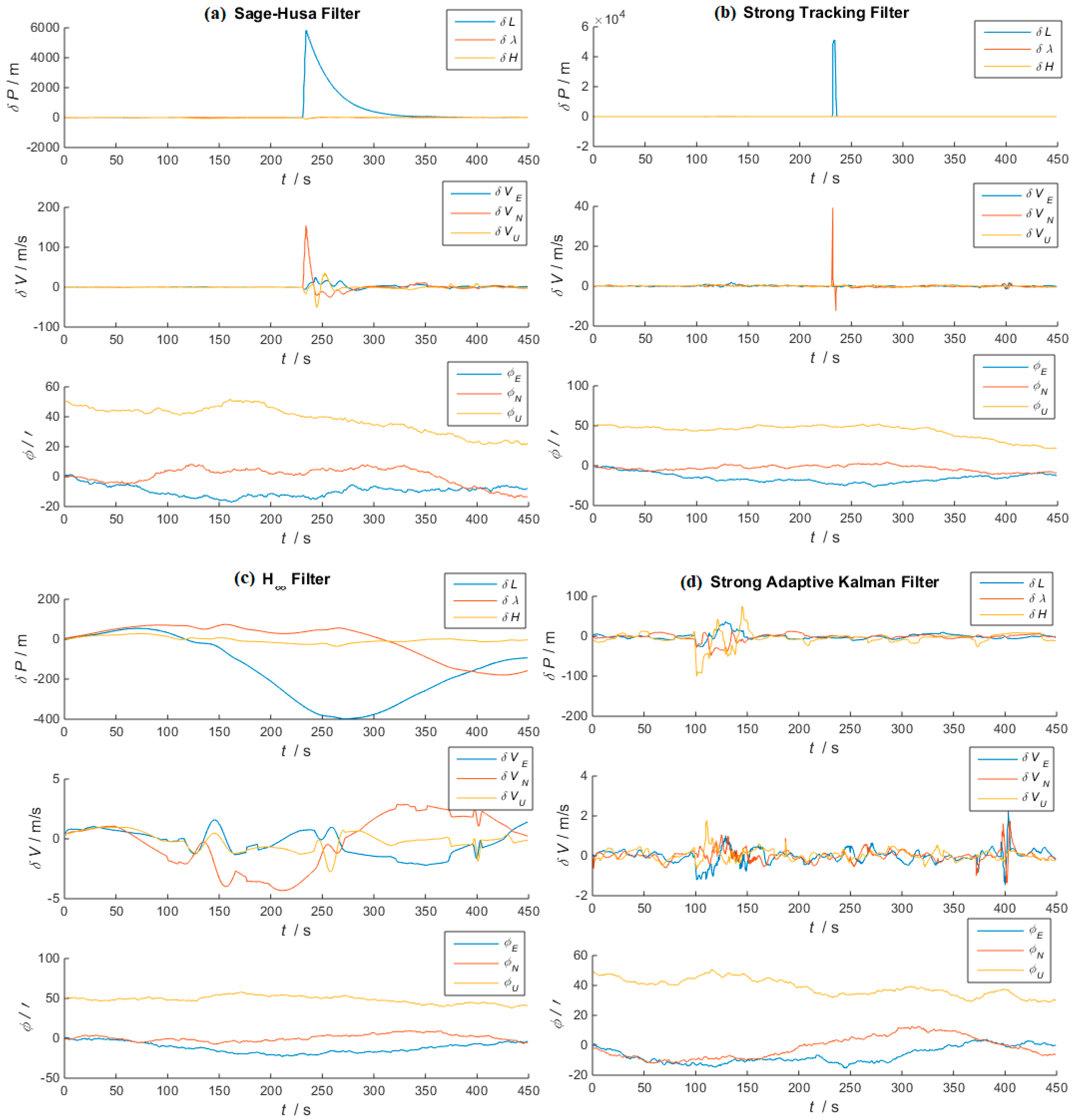
Figure 5.
(a) 3D trajectory diagram; (b) diagram of eastward velocity, northward velocity and upward velocity.
Figure 5.
(a) 3D trajectory diagram; (b) diagram of eastward velocity, northward velocity and upward velocity.

Figure 6.
3D trajectory diagram (a) SHAKF; (b) STF; (c) H∞ filter; (d) SAKF.


Table 1.
Configuration of sensors and initial errors.
| Type of Parameter | Parameter | Value |
|---|---|---|
| Initial error of attitude | Pitch; Roll; Yaw | 30′, 30′, 50′ |
| Initial error of position | Longitude; Latitude; Height | 10 m, 10 m, 20 m |
| Initial error of velocity | Horizontal velocity; Vertical velocity | 0.1 m/s, 0.5 m/s |
| Precision of gyroscope | Drift | 5°/h |
| Random walk | ||
| Precision of accelerometer | Bias | 20 mg |
| Random walk | ||
| Initial error of attitude | Horizontal precision | 5 m |
| Vertical precision | 10 m | |
| Precision of velocity | 0.2 m/s |
Table 2.
The root mean square (RMS) obtained by the output of four algorithms in scene 1 (250 s~300 s).
Table 2.
The root mean square (RMS) obtained by the output of four algorithms in scene 1 (250 s~300 s).
| Algorithm | Attitude θ, φ, γ/′ | Velocity VE, VN, VU/m/s | Horizontal Position λ, L/m | Vertical Position H/m |
|---|---|---|---|---|
| SHAKF | 21.2, 19.9, 30.4 | 7.64, 5.57, 2.42 | 47.3, 73.7 | 20.8 |
| STF | 48.4, 18.8, 67.9 | 0.27, 1.04, 0.13 | 6.22, 5.14 | 9.05 |
| H∞ | 26.4, 9.01, 47.5 | 10.2, 7.06, 2.15 | 35.4, 39.9 | 17.3 |
| SAKF | 30.4, 17.5, 59.6 | 0.49, 0.27, 0.31 | 5.15, 5.19 | 6.65 |
Table 3.
The RMS obtained by the output of four algorithms in scene 2 (100 s~150 s).
| Algorithm | Attitude θ, φ, γ/′ | Velocity VE, VN, VU/m/s | Horizontal Position λ, L/m | Vertical Position H/m |
|---|---|---|---|---|
| SHAKF | 13.6, 5.50, 43.9 | 0.58, 0.66, 0.22 | 28.7, 28.8 | 10.5 |
| STF | 17.1, 6.59, 45.6 | 0.70, 0.80, 0.45 | 31.8, 41.9 | 10.7 |
| H∞ | 12.7, 3.81, 49.7 | 0.88, 1.79, 0.59 | 22.1, 32.4 | 4.46 |
| SAKF | 6.14, 1.59, 41.7 | 0.65, 0.48, 0.54 | 10.4, 13.1 | 8.65 |
Table 4.
Initial Error of UAV.
| Type of Error | Value |
|---|---|
| Horizontal attitude | 30′ |
| Yaw | 50′ |
| Horizontal position | 10 m |
| Height | 20 m |
| Horizontal velocity | 0.1 m/s |
| Vertical velocity | 0.5 m/s |
Table 5.
Comparison of filtering errors.
| Time (s) | Error of STF (m) | Error of H∞ (m) | Error of SAKF (m) |
|---|---|---|---|
| 500 | 10.4 | 21.5 | 9.7 |
| 800 | 13.7 | 34.9 | 12.4 |
| 1000 | 8.4 | 14.4 | 7.9 |
| 1800 | 14.5 | 32.4 | 10.6 |
| 2500 | 4.6 | 15.5 | 4.1 |
© 2019 by the authors. Licensee MDPI, Basel, Switzerland. This article is an open access article distributed under the terms and conditions of the Creative Commons Attribution (CC BY) license (http://creativecommons.org/licenses/by/4.0/).
Share and Cite
MDPI and ACS Style
Huang, T.; Jiang, H.; Zou, Z.; Ye, L.; Song, K. An Integrated Adaptive Kalman Filter for High-Speed UAVs. Appl. Sci. 2019, 9, 1916. https://doi.org/10.3390/app9091916
AMA Style
Huang T, Jiang H, Zou Z, Ye L, Song K. An Integrated Adaptive Kalman Filter for High-Speed UAVs. Applied Sciences. 2019; 9(9):1916. https://doi.org/10.3390/app9091916
Chicago/Turabian StyleHuang, Tiantian, Hui Jiang, Zhuoyang Zou, Lingyun Ye, and Kaichen Song. 2019. "An Integrated Adaptive Kalman Filter for High-Speed UAVs" Applied Sciences 9, no. 9: 1916. https://doi.org/10.3390/app9091916
Note that from the first issue of 2016, this journal uses article numbers instead of page numbers. See further details here.