Landslide Prediction with Model Switching †


Computer Science and Information Engineering, National Chung Cheng University, No. 168, Sec. 1, University Rd., Minhsiung, Chiayi 62102, Taiwan
*
Author to whom correspondence should be addressed.
†
This paper is an extended version of paper published in the 2017 IEEE Conference on Dependable and Secure Computing, held in Taipei, Taiwan, 7–10 August 2017.
Appl. Sci. 2019, 9(9), 1839; https://doi.org/10.3390/app9091839
Submission received: 30 March 2019
/
Revised: 27 April 2019
/
Accepted: 28 April 2019
/
Published: 4 May 2019
(This article belongs to the Special Issue Machine Learning Techniques Applied to Geoscience Information System and Remote Sensing)
Abstract
:Landslides could cause huge damages to properties and severe loss of lives. Landslides can be detected by analyzing the environmental data collected by wireless sensor networks (WSNs). However, environmental data are usually complex and undergo rapid changes. Thus, if landslides can be predicted, people can leave the hazardous areas earlier. A good prediction mechanism is, thus, critical. Currently, a widely-used method is Artificial Neural Networks (ANNs), which give accurate predictions and exhibit high learning ability. Through training, the ANN weight coefficients can be made precise enough such that the network works in analogy to a human brain. However, when there is an imbalanced distribution of data, an ANN will not be able to learn the pattern of the minority class; that is, the class having very few data samples. As a result, the predictions could be inaccurate. To overcome this shortcoming of ANNs, this work proposes a model switching strategy that can choose between different predictors, according to environmental states. In addition, ANN-based error models have also been designed to predict future errors from prediction models and to compensate for these errors in the prediction phase. As a result, our proposed method can improve prediction performance, and the landslide prediction system can give warnings, on average, 44.2 min prior to the occurrence of a landslide.
1. Introduction
Landslides are natural disasters which can cause huge damage to properties and severe loss of lives. Many studies have focused on how to detect and monitor landslides. Though landslide detections could be performed in real-time, there might not be enough time to react, so as to save human lives and properties. In order to minimize the losses caused by landslides, an early prediction mechanism, with pre-warnings, is necessary. Once the system can give an alarm in advance, people would have more response time to evacuate before the landslide occurs.
There are several problems in landslide prediction. First, just as in most safety-critical applications, landslide prediction also exhibits the same data imbalance problem, where the class of stable data has much more data than the class of unstable data. Stable data, here, refers to the normal conditions (where there is no landslide), while unstable data represents landslide-related information. Second, a low true-positive rate (TPR) problem is often found in safety-critical applications, because of the interference in learning between two or more classes in the datasets. For example, learning from the normal stable conditions often affects the learning from the unstable (landslide) conditions, thus resulting in a low TPR. Third, predictive applications are often faced with the problem of determining an appropriate prediction horizon; that is, the size of the time window of past history to be used for predictions. Finally, real-time applications face the problem of determining when to re-train the models.
To address the above-mentioned four problems existing in landslide prediction, this work provides a total solution in the form of an early warning system, called the Model Switch-based Landslide Prediction System (MoSLaPS). To address the data imbalance problem, we adapt the popular Adaptive Synthetic Sampling (ADASYN) method [1] to landslide prediction. To address the low TPR problem, we propose a novel event-class model switch predictor design that significantly improves TPR. To address the problem of customizing the prediction horizon, we also propose a novel dynamic tuning method for the prediction horizon, in order to achieve the goal of early warning. To address the problem of determining model re-training time, we propose a novel learning-based re-training method, based on an error model which considers both the long-term and short-term accumulated errors. Errors are also predicted, so re-training can be done earlier in preparation for future data changes; as a result of which, our proposed system can achieve the goal of early warning.
2. Related Work
Landslide prediction methods can be classified into three types: Image analysis, machine learning, and mathematical evaluation models. Table 1 shows a comparison among these types of methods. First, image analysis uses Geographic Information Systems (GIS), which can collect, store, manage, and analyze geographical data. By analyzing disaster data, such as history of landslides and data on land development for agriculture, the risk of landslides can be predicted. The probability of landslides is variable, as it is based on the number of layers of data used for analysis. Second, machine learning techniques, such as Bayesian networks [2], neural networks [3], or genetic algorithm [4], use computational intelligence to calculate the probability of landslides. These methods incorporate different factors that might cause landslides to evaluate the probability of landslide occurrence. They are not real-time, because they require huge computational times for prediction. Finally, mathematical evaluation models use a single evaluate equation, such as Factor of Safety (FS) [5]. A hazard model is combined with the physical concepts of mechanics and hydrographic data for the stability of slopes. It is easy for simulation and fits a wide range of environments, but it is difficult to obtain the whole hydrographic data as groundwater elevation is difficult to measure.
Landslides occur when the down-slope shear stress is large. As shown in Equation (1) [5], the Factor of Safety (FS) refers to the stability of the soils. It takes physical properties, including rainfall, slope, and soil properties, into consideration. It can easily predict landslides with the trend of each parameter. Therefore, to predict landslides, a FS equation is matched with these attributes. Three regions of the FS value, based on the SHALSTAB model [6], are defined to distinguish between the dangerous levels of a slope, as shown in Table 2. The Stable Region is classified as the stable class and the Marginally Stable and Actively Unstable Regions are classified as the unstable class. Based on the classes, different training samples are used to train multiple neural network predictors.
with
- C: The effective coefficient (kPa);
- R: The rainfall intensity (mm/hr);
- T: The soil transmissivity (mm/hr);
- Z: The soil depth (m);
- : The density of water (kg/m);
- : The density of soil (kg/m);
- : The internal friction angle of the slope material (degree);
- : The slope gradient (degree); and
- : The specific contributing area [5].
Of particular mention is the work done by Lian et al. [7,8] on landslide displacement prediction using Prediction Intervals (PIs) and an ANN switched prediction method. The authors employed K-means clustering for dividing the landslide data into two classes; namely, a majority class (stationary points) and a minority class (mutational points). Then, a weighted Extreme Learning Machine (ELM) classifier was used to construct the switch rules. Finally, bootstrap and kernel-based ELMs were applied to construct the PIs. This work was concerned with how the displacements are predicted accurately and early. In contrast, our work is focused on how landslides can be actually predicted accurately and early. Not only is the goal different, the methods or techniques used or proposed are also quite different. We employ a very popular mathematical estimation model for landslide prediction, as defined above (namely, the SHALSTAB model and the factor of safety). We use ANN models for the model switching, as well as for the predictions. We adapt ADASYN for resolving the data imbalance problem. We also propose novel methods for model retraining and prediction horizon tuning. Details are given in the next section.
3. Model Switched Landslide Prediction System
A total solution for landslide prediction with early warnings is proposed in this work. The design of the proposed Model Switched Landslide Prediction System (MoSLaPS) is shown in Figure 1. It consists of two parts; namely, Physical Entities and Computation Elements. In the Physical Entities, environmental data, such as rainfall, soil moisture, and slope, are collected by sensor nodes. Coordinator nodes integrate the sensed data and transmit them to the Computation Elements through Zigbee transmitters. The Computation Elements consists of a SHALSTAB Model, a Switch-based Prediction Model, and an Accurate Early Warning System, as described in the following.
- SHALSTAB ModelThe SHALSTAB model takes the sensed environmental data, including rainfall, soil moisture, and slope, from the Physical Entities and evaluates the Factor of Safety, using Equation (1). Over time, the FS values are recorded as , which is the input to the Accurate Early Warning System to predict the occurrence of landslides.
- Switch-based Prediction ModelFrom historical environmental data, the proposed system consists of two prediction models to learn two different data patterns; namely, the stable pattern and the unstable pattern. To switch between the different prediction models, a neural network classifier is designed to predict the future class. The Switch-based Prediction Model can improve the prediction accuracy when the neural network classifier switches the prediction models accurately. The detailed technique is described in Section 3.3.
- Accurate Early Warning SystemThe accurate early warning system consists of a data analysis server and alert services. The data analysis server uses the above-described switch-based prediction model to predict landslides. The input data, , is used to predict future FS values, denoted as . For each predicted FS value, there is a difference between the predicted FS and the actual FS calculated using Equation (1). This difference is called prediction error. The data analysis server will assess the applicability of the prediction model, according to the trend of prediction errors. If the error exceeds a pre-defined threshold, it means the prediction model is not suitable for the environment at that time and the predicted results have large prediction errors. Thus, based on the error measurement and a given error tolerance threshold, the prediction model is re-trained. The entire process will be described in Section 4. If a predicted FS value, , is smaller than 1, then it is estimated that a landslide will occur after k time slots [9]. Thus, alert services can send an alert in advance.
The details of the prediction models, model switching, and early warning system will be introduced in the rest of this section.
3.1. Prediction Model Design
To predict the future FS, a feed-forward Back-Propagation Neural Network (BPNN) is employed as the prediction model. A BPNN is a powerful computation system, created by generalizing the Widrow-Hoff learning rules [10] into a multi-layer with a non-linear differential transfer function network. The complex network connections imply that the high learning and reasoning ability of BPNN can be applied to deal with problems with high complexity. Figure 2 shows the framework of a BPNN-based prediction model.
Training Method for Time-Series Based BPNN
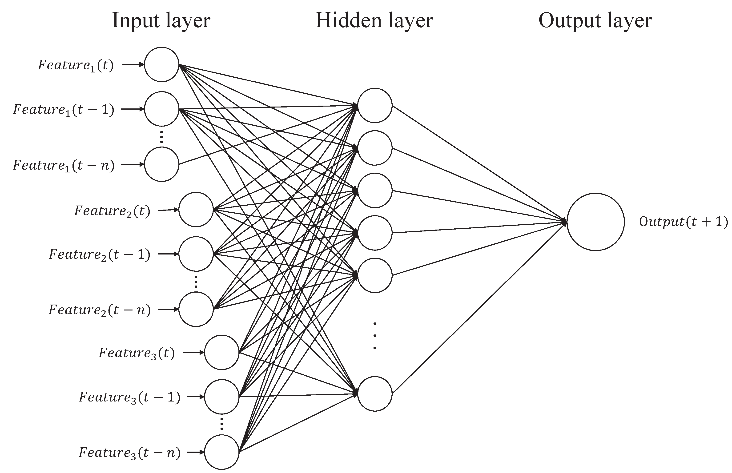
The basic computational procedure of a BPNN is explained to provide a basic description of the type of ANN that is implemented here. Figure 3 shows the basic structure of a time-series based BPNN. There are three types of layers: input, hidden, and output layers. In the input layer, time-series input for time slots to t, corresponding to a specific feature, such as factor of safety, rainfall, and soil moisture, is taken as input data. Each pair of nodes in the adjacent layers are linked by a weight. The values in all nodes in a previous layer and the weights are multiplied and accumulated as the input for a node of the next layer. The inputs are, then, given to an activation function to calculate the output value of the node. Repeating the above operations, layer by layer, from input layer to output layer, the final output can be derived.
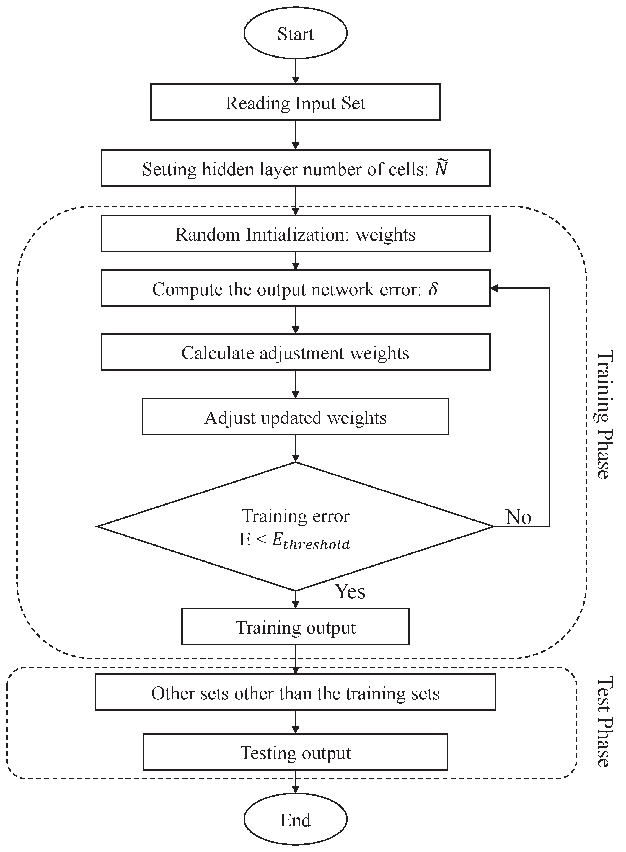
Algorithm 1 has a complete description as a prediction model; the following equations explain the functions that are used in this algorithm. At first, the previous FS is used to predict the future FS by a BPNN model. To dynamically determine suitable weights for different FS, a back-propagation method is applied to train and update the weights before prediction, in order to completely illustrate the details of back propagation method. Given the training sample, , where is the impact factor and is the training target, the general mathematical model of a standard single hidden layer feed-forward network with hidden neurons is shown in Equation (2).
where is the jth output of the BPNN, is the weight of the connection from the input neurons to the ith hidden neuron, and is an activation function that represents how much adjustment the output should be from the neuron, based on the sum of the input. The activation function used in our BPNN model is depicted in Equation (3); namely, the sigmoid function. The sigmoid function, also called the logistic function, is a commonly-used activation function which has an output range from 0 to 1.
The difference between the prediction result and the actual result is called the prediction error. In order to reduce prediction error, the weights need to be updated. The Levenberg-Marquardt (LMA) [11] method has the fastest convergence and the lowest mean square error. Therefore, LMA is selected as a training function to calculate the output network error and adjustment weight W. It is depicted in Equation (4):
where represents the weight matrix in the kth iteration, J is the Jacobian matrix [12] that contains the network error for weight and the first-order differential of weight, I is the unit matrix, is the network output error, and u is a constant. LMA can dynamically adjust the constant u to reduce the network output error .
| Algorithm 1: Prediction Model Algorithm. |
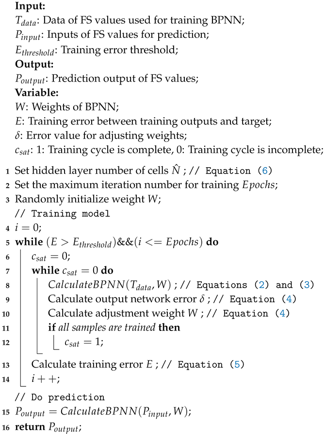 |
After the training phase, the training error E is calculated by Equation (5), to determine whether the training step has reached convergence. If it is not less than the training error threshold, , the training phase is restarted.
where:
- : Target FS value of training sample i;
- : BPNN output FS value of training sample i; and
- N: Number of training samples.
Considering the training time in our proposed re-training process, the number of outputs, , is set to 1 to avoid a long training time. This means that only one prediction result per iteration will be obtained, by taking the past FS value as input.
The number of neurons in the hidden layer, denoted as , is determined based on the following experience rule [13]:
- The number of neurons in the first hidden layer is calculated using (6):
3.2. Imbalanced-Class Prediction Design
Class balance enhancements are needed to handle training samples with an unbalanced class distribution [14]. The Adaptive Synthetic Sampling (ADASYN) method [1] is used here for balancing the imbalanced data (i.e., data is pre-processed using ADASYN), and then the processed dataset are used to train the event-class predictor, which is also a BPNN model. In the following, the ADASYN algorithm is described as follows.
Data Pre-Processing Using ADASYN Algorithm
The ADASYN algorithm can improve the data imbalance problem by synthetically creating new samples from the unstable class by linear interpolation between existing unstable class samples. This approach, by itself, is known as the Synthetic Minority Over-sampling Technique (SMOTE) method [15]. ADASYN is an extension of SMOTE, creating more samples in the vicinity of the boundary between the two classes than in the interior of the unstable class.
To create more synthetic data for the unstable class, FS, rainfall, and soil moisture are used as the training data and the corresponding class label, , is constructed according the classification region. Given the training samples , , where , is the FS value, is the rainfall, is the soil moisture, is the slope gradient, and is the class label. The training samples, , are classified by Equation (7). For , classifies as stable class. On the other hand, if , then classifies as unstable class. After is classified, the class label, , is set by Equation (8). If , is set as 0. If , is set as 1.
To adjust class balance, the degree of class imbalance is needed to be calculated by Equation (9):
where
- : The size of unstable class examples; and
- : The size of stable class examples.
Furthermore, the default level, , which is the threshold for the level of maximum class imbalance tolerated, also needs to be determined beforehand. If the current d is smaller than the threshold degree, , then the number of synthetic data samples that need to be generated for the unstable class is calculated using Equation (10):
where is a parameter used to specify the desired balance level after generation of the synthetic data: means a fully balanced data set is created after the generalization process.
For each , K nearest neighbours can be found by using the Euclidean distance. The ratio , defined in Equation (11), which represents the number of stable-classified in the K nearest neighbours, and its normal form, , defined in Equation (12), are calculated, where is called a density distribution of , ().
where is the number of samples in the K nearest neighbours of that belong to the stable class; therefore, .
Thus, the number of synthetic data samples that need to be generated for each unstable class sample, , can be calculated by Equation (13).
where R is the total number of synthetic data samples that need to be generated for the unstable class, as defined in Equation (10).
By random, the program chooses one unstable data sample, , from the K nearest neighbours for to generate new synthetic samples, , by Equation (14). This procedure is repeated times to produce new synthetic samples.
where
- : The difference vector; and
- : A random number .
3.3. Switch-Based Prediction Model Design
To address the issue of imbalanced data between the unstable and stable classes, a switch-based neural network prediction algorithm is proposed, as detailed in Algorithm 2.
The environmental factors, including rainfall, soil moisture, and slope gradient, are used to calculate the FS values, , using the SHALSTAB model. Given the environmental samples , where , is the rainfall, is the soil moisture, and is the slope gradient, the FS values, , are calculated given the set of all training samples, , where . Then, the corresponding class labels , , can be constructed and classified by Equations (7) and (8). To construct the BPNN models for different data patterns, the calculated FS need to be classified in two subsets, as follows:
where is the set of FS values for , in , and is the set of FS values for , in ; so that and .
| Algorithm 2: Switch-based Neural Networks Prediction Algorithm. |
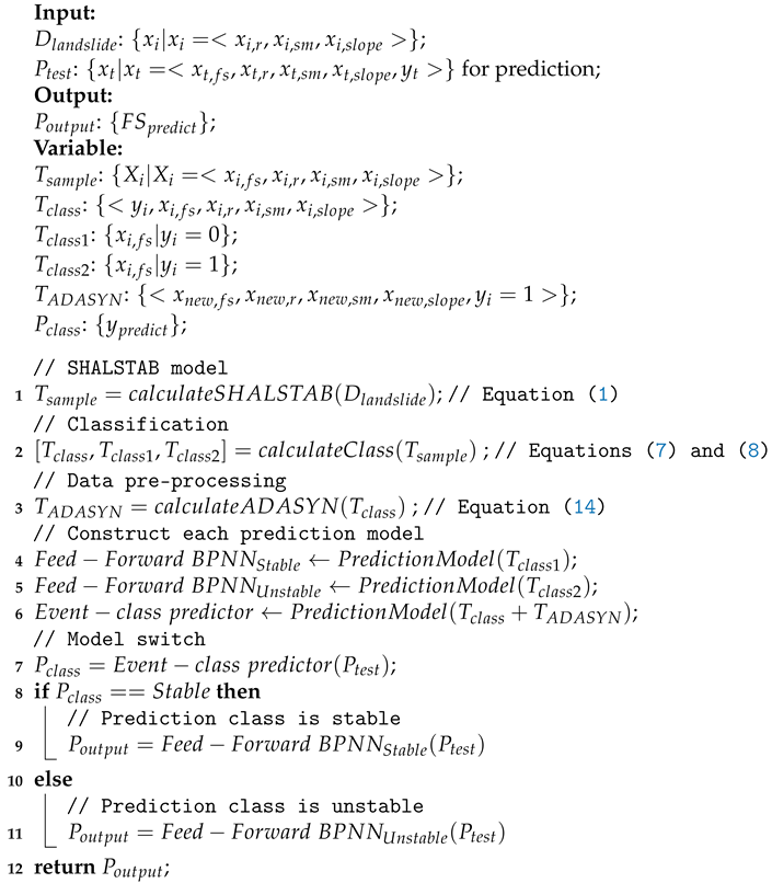 |
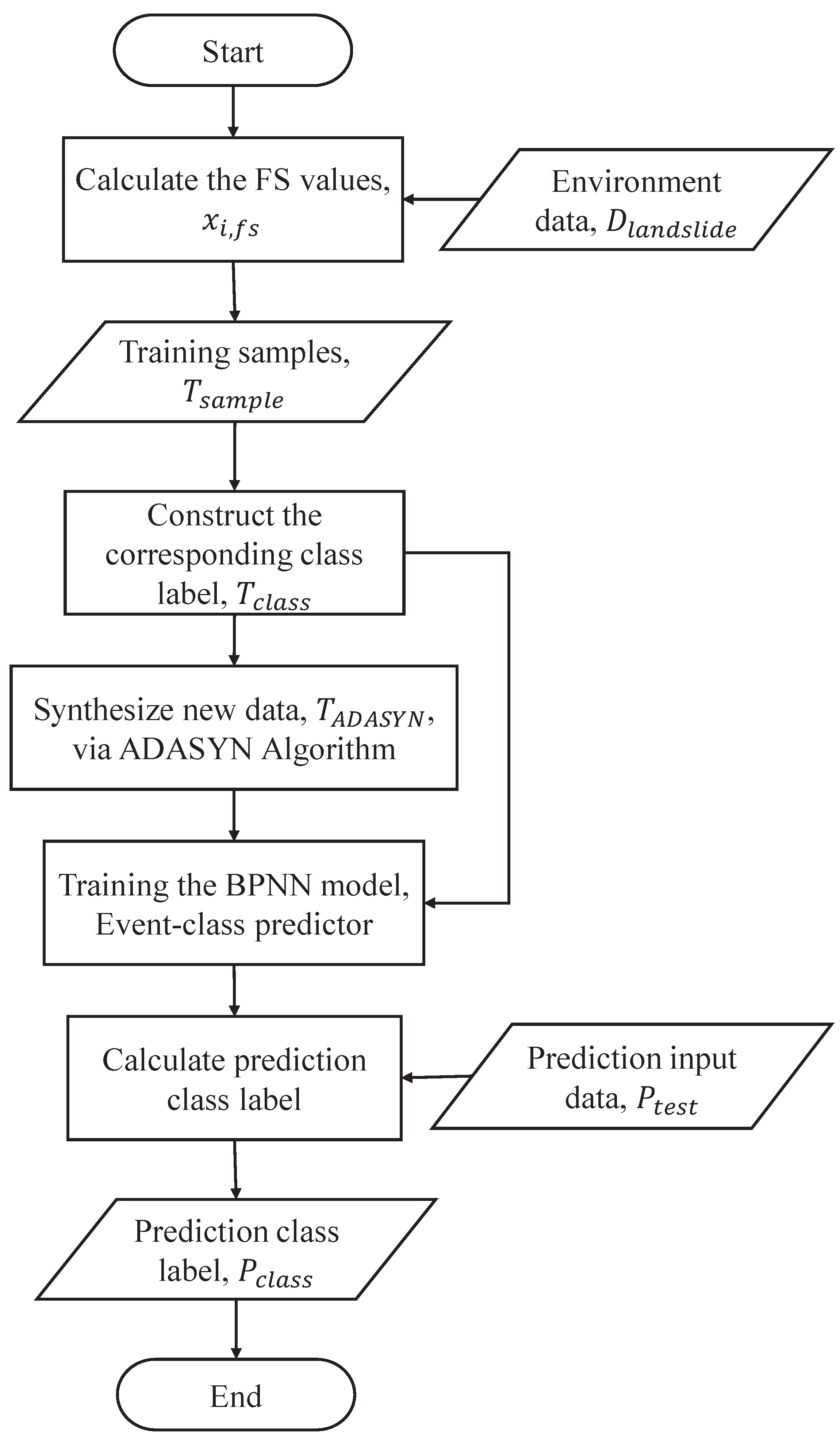
Here, the ADASYN algorithm is used to produce new synthetic samples for the unstable class, in order to balance the sizes of the two classes. The processed dataset, , is used to predict the future class using a BPNN model. The event-class predictor can switch between the different models, according to the predicted class. As shown in Figure 4, the steps of the event-class predictor are as follows.
First, is selected to construct the synthetic dataset for balancing class distribution by the ADASYN algorithm, where are the new synthetic samples, , and represents that the synthetic class label is unstable class. The synthetic include , the new synthetic FS value; , the new synthetic rainfall; , the new synthetic soil moisture; and , the new synthetic slope gradient. Both of the classes and are integrated into the training set of the event-class predictor. Second, the event-class predictor is constructed using the BPNN model. Finally, the event-class predictor is used to predict the future class label, , for the testing phase, where represents that the prediction class label is stable and represents that the prediction class label is unstable.
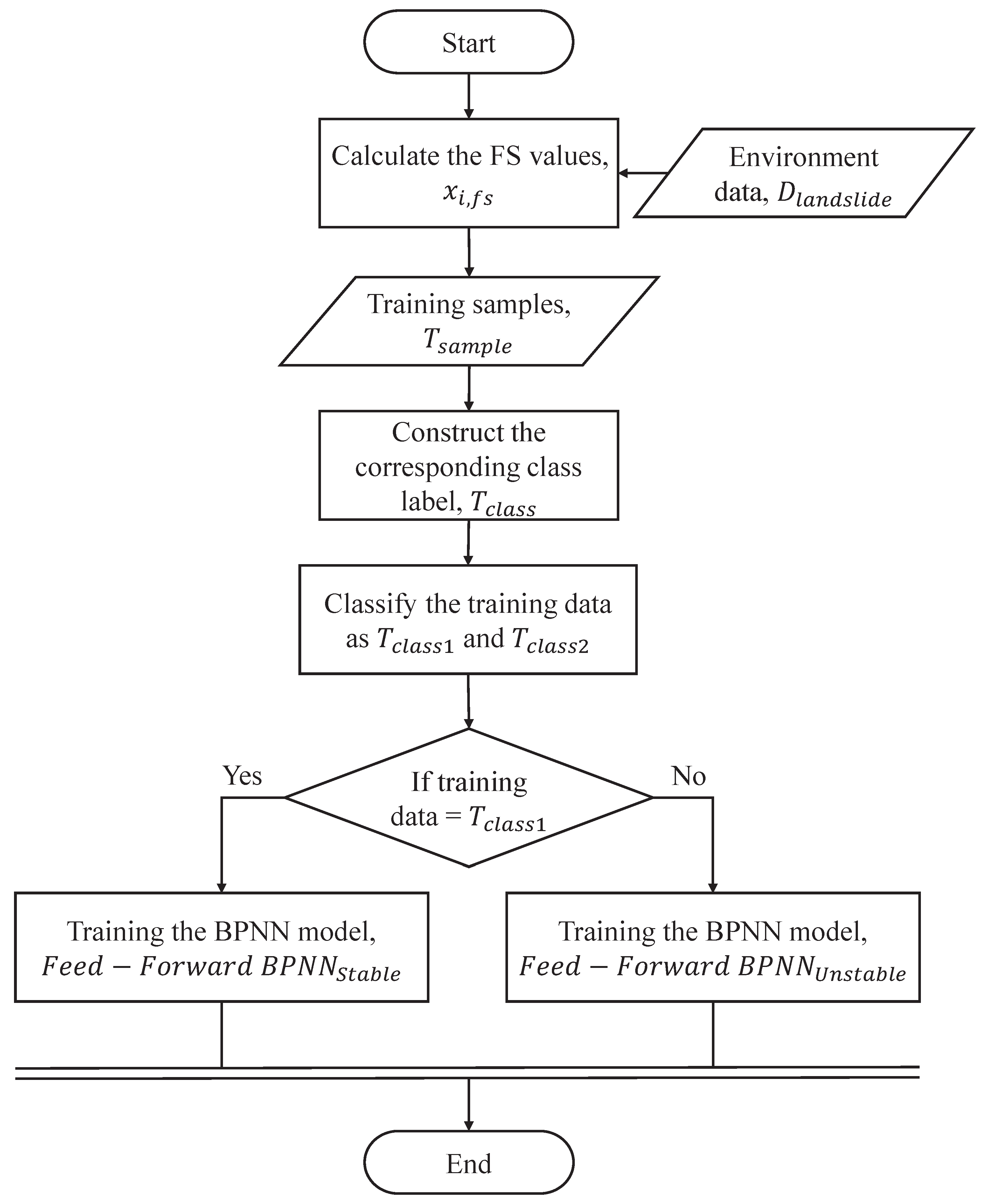
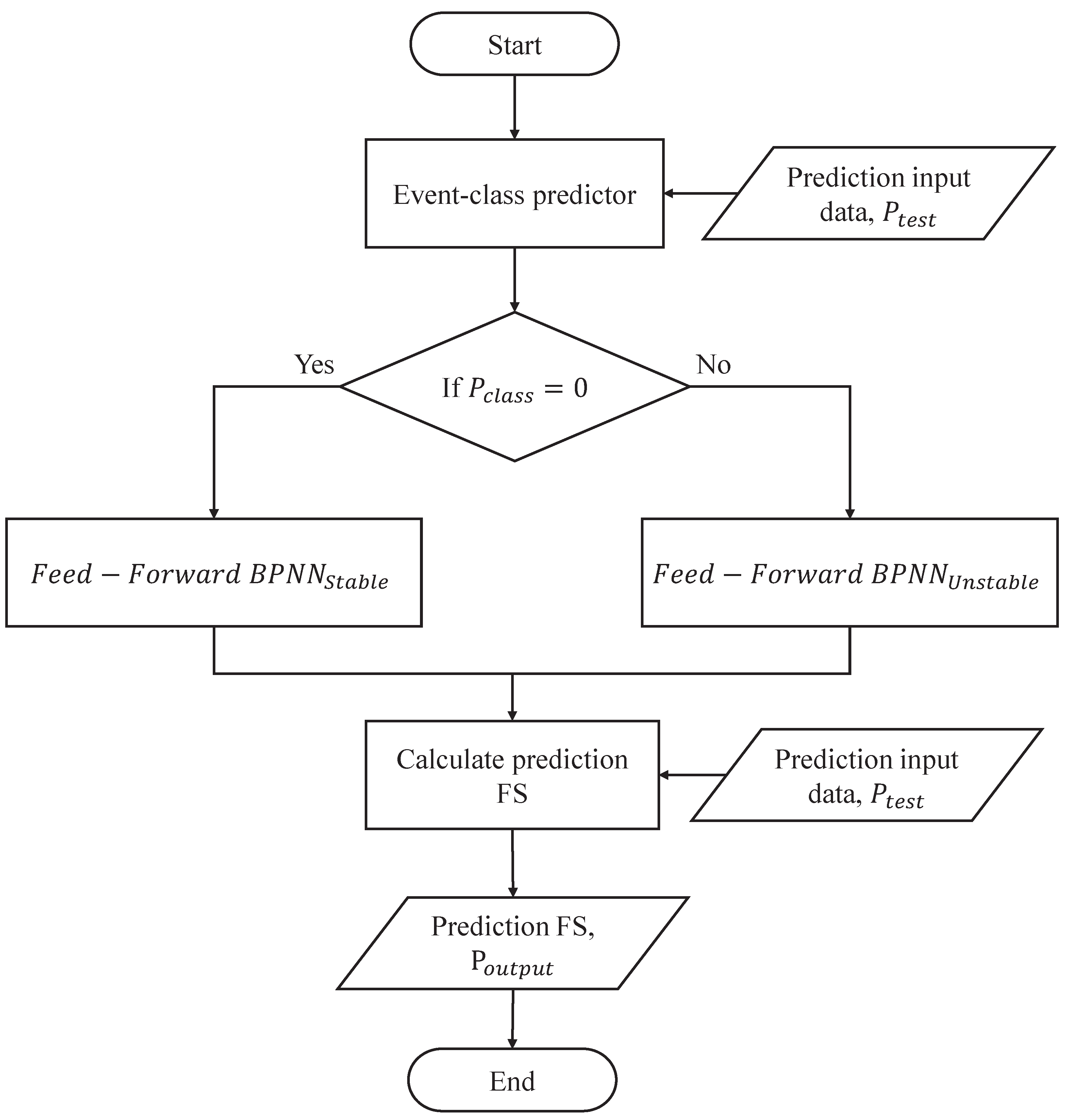
The aim of our proposed method is to construct different pattern predictors, as shown in Figure 5. The steps of different pattern predictors are as follows. First, is used as training data to train a BPNN model. After training, the BPNN model is the stable pattern of (i.e., ). On the other side, is applied as training data to train another BPNN model. After training, the BPNN model is the unstable pattern of (i.e., ). Thus, two BPNNs are built to deal with different patterns. As shown in Figure 6, this procedure can switch different pattern predictors, according to the predicted class, , that is obtained by the event-class predictor. When , the testing data, , is applied to predict the future FS using , where , is the testing data of the FS value, is the testing data of the rainfall, is the testing data of the soil moisture, is the testing data of the slope gradient, and is the testing data of the corresponding class label. On the other side, when , is employed to predict the future FS using . Finally, the predicted FS, , can be obtained by using the proposed Switch-based Prediction Model.
The main contribution of this work is that the proposed method can make highly accurate predictions, even in the case of highly imbalanced data. Two techniques were employed, ADASYN and an event-class predictor.
4. Accurate Early Warning System Design
To ensure the switch-based neural networks prediction model can be precise in a changing environment, an accurate early warning system is designed, as shown in Figure 7. It is divided into two parts: A learning-based re-training flow, as described in Section 4.1, and a Prediction Horizon tuning flow, as shown in Section 4.2.
4.1. Learning-Based Re-Training Flow
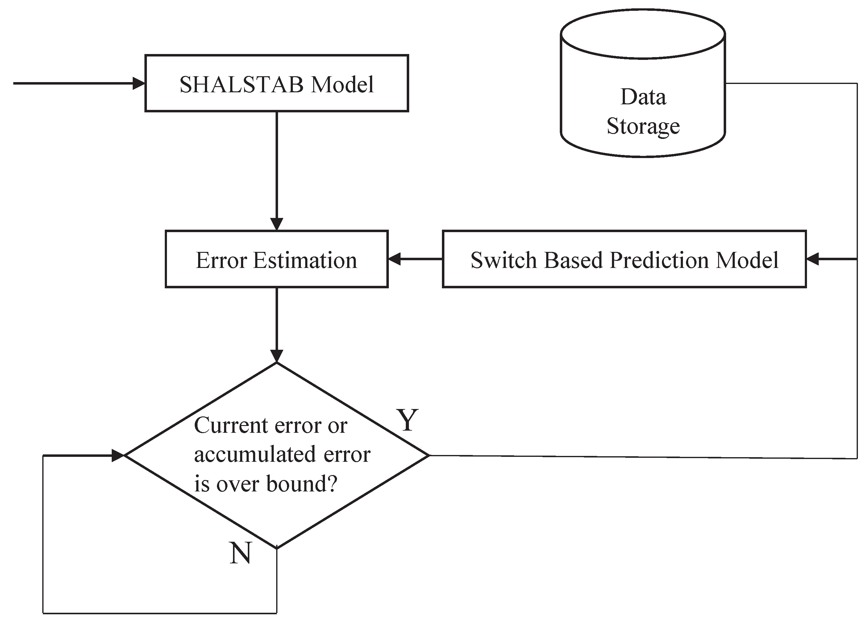
Figure 8 shows the flow of learning-based re-training. The determination of ret-raining is based on the error estimation. The error estimation process calculates the average error of all () pairs in an error-estimation window (EEW). For each period of the EEW, this procedure compares the average error, , of two error estimation windows, and , and the accumulated error, , to check the two conditions for re-training. Equations (17) and (18) give the two conditions under which the prediction model needs to be re-trained, where is the coefficient of interval error used to specify the short-term tolerable error range, which is equal to the size of the prediction horizon in our work. If the difference of between two continuous is too large, the prediction model will be re-trained, due to the high variability of the input pattern that the original prediction model could not predict. Here, is the coefficient of accumulated error used to specify the long-term tolerable error range (here, long-term means since epoch). If the , compared to average error of the prediction model, , is too large, the prediction model will also be re-trained, as the prediction results are becoming inaccurate. This further implies that the environment is changing with time, and that adaptation is needed. and are calculated using Equations (19) and (20), respectively.
4.2. Prediction Horizon Tuning
In the re-training flow, the error estimation results are utilized further to tune the prediction horizon. The advantages of a variable-length prediction horizon (PH) are as follows:
- The occurrence of landslides can be predicted earlier; and
- The number of false predictions can be reduced.
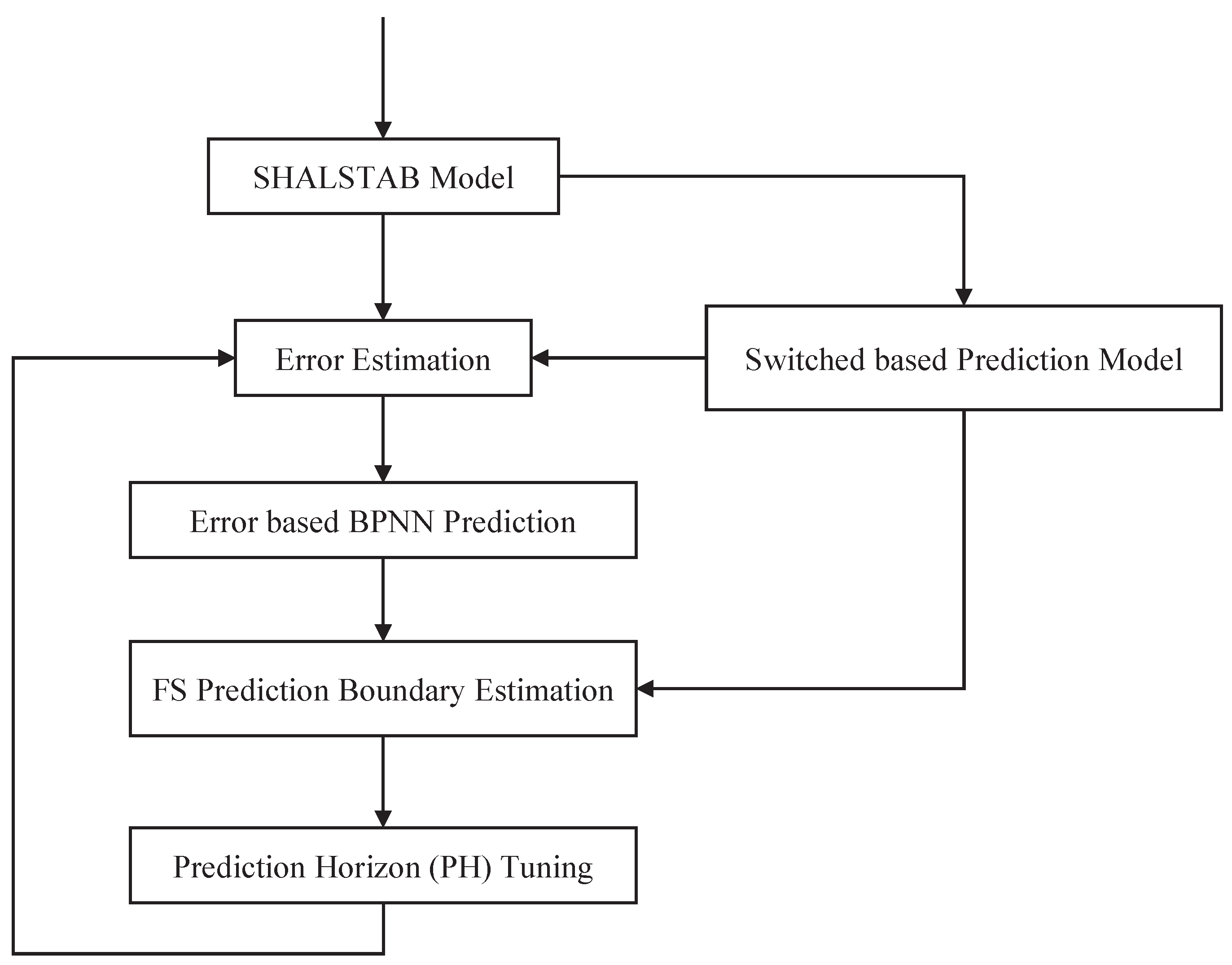
The prediction horizon tuning flow is shown in Figure 9. Prediction errors are non-linear, and the prediction model is applied (as described in Section 3.1) in order to learn the inherent pattern for predicting future errors, . In this way, the size of the PH is set to predict the occurrence of landslides earlier. Then, the future target ranges, , can be determined by Equation (21). If the range of , this system can send alerts in advance.
To decide whether the size of the PH is tuned, error boundary estimation is needed. As the program already has the predicted error, , and the predicted FS, , then the predicted lower bound, , can be estimated by Equation (22). According to the estimated results, the tuning is performed based on the following rules:
- If there is no lower than the lower bound of Stable Class (i.e., 1.3), for every time point in the prediction horizon, the size of the prediction horizon is increased by 1; and
- If there exists one lower than the lower bound of Stable Class (i.e., 1.3), for every time point in the prediction horizon, the size of prediction horizon is reset to the default value.
Based on the above rules, we make our method a little more flexible for the landslide prediction scenario with variable-length prediction horizon.
5. Experiments
In this section, evaluations of the proposed method for landslide prediction are presented. First, the experimental datasets used for the experiments are introduced. Then, the experimental results are illustrated. All experiments were carried out using the MATLAB programming language on a PC with an Intel Core™ i7-3770 CPU @ 3.40GHz and 16 GB RAM, running the Windows 10 (64-bit) OS.
5.1. Experimental Datasets
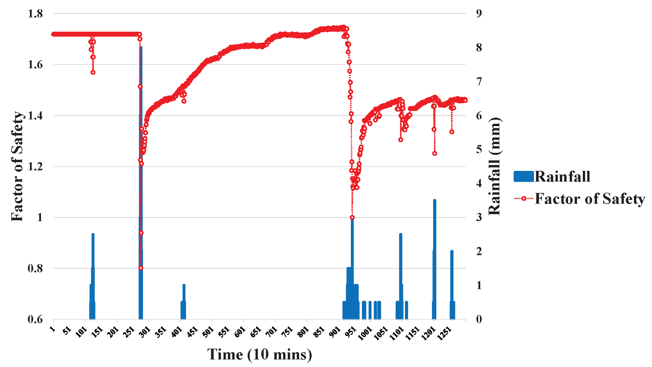
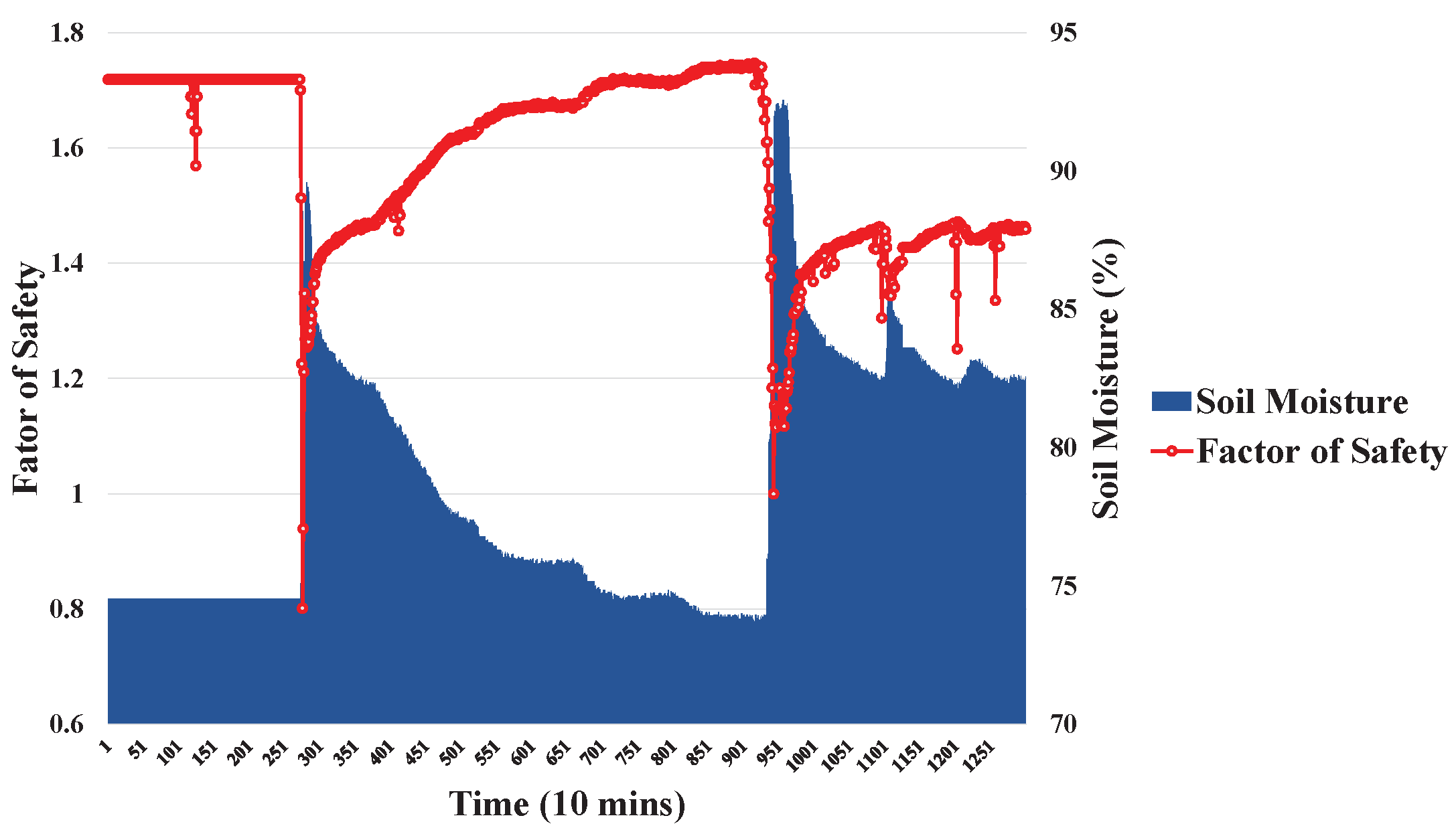
Historical environmental monitoring datasets from the Shen-Mu station [16] were selected as a case study. Landslides are mainly influenced by rainfall and soil moisture. Using the FS, the occurrence of a landslide is estimated. The monitoring dataset of the Shen-Mu station is shown in Figure 10 and Figure 11. Figure 10 and Figure 11 show the relationships between rainfall and FS, and between soil moisture and FS, respectively. When rainfall and/or soil moisture increase, the FS decreases and the slope becomes unstable.
In the Shen-Mu datasets [16], data was recorded once per 10 min, and was collected in 2016. The program randomly selected 10 sets of samples, where each set had 1300 samples. Each dataset was further divided into two parts, the training set (75%) and the test set (25%). Note that the original data were used as input; that is, they were not normalized, because we needed to calculate the FS according to the SHALTAB model, as given in Equation (1).
Firstly, an evaluation of imbalanced-class prediction is described. Then, it is shown how the prediction accuracy is increased due to the proposed MoSLaPS.
5.2. Evaluation of Event-Class Prediction
ADASYN [1] was applied for data pre-processing in this program. It synthetically created new samples from the unstable class to balance the distribution of the data, if required. In the ADASYN algorithm, the desired level of balance, , could be adjusted to control the number of new synthetic samples, which were needed when .
Our event-class predictor used ADASYN [1] for imbalanced data processing. After data pre-processing, the processed dataset was used to train the event-class predictor (i.e., a BPNN model). To evaluate the event-class predictor, several performance indicators were applied and defined, as follows:
If the prediction class was unstable and the actual class was also unstable, then the result was said to be a True Positive (TP). If the prediction class was stable and the actual class Was also stable, then the result was said to be a True Negative (TN). If the prediction class was unstable and the actual class was stable, then the result was said to be a False Positive (FP). If the prediction class was stable and the actual class was unstable, then the result was said to be a False Negative (FN). Table 3 shows the classification of the above four different categories.
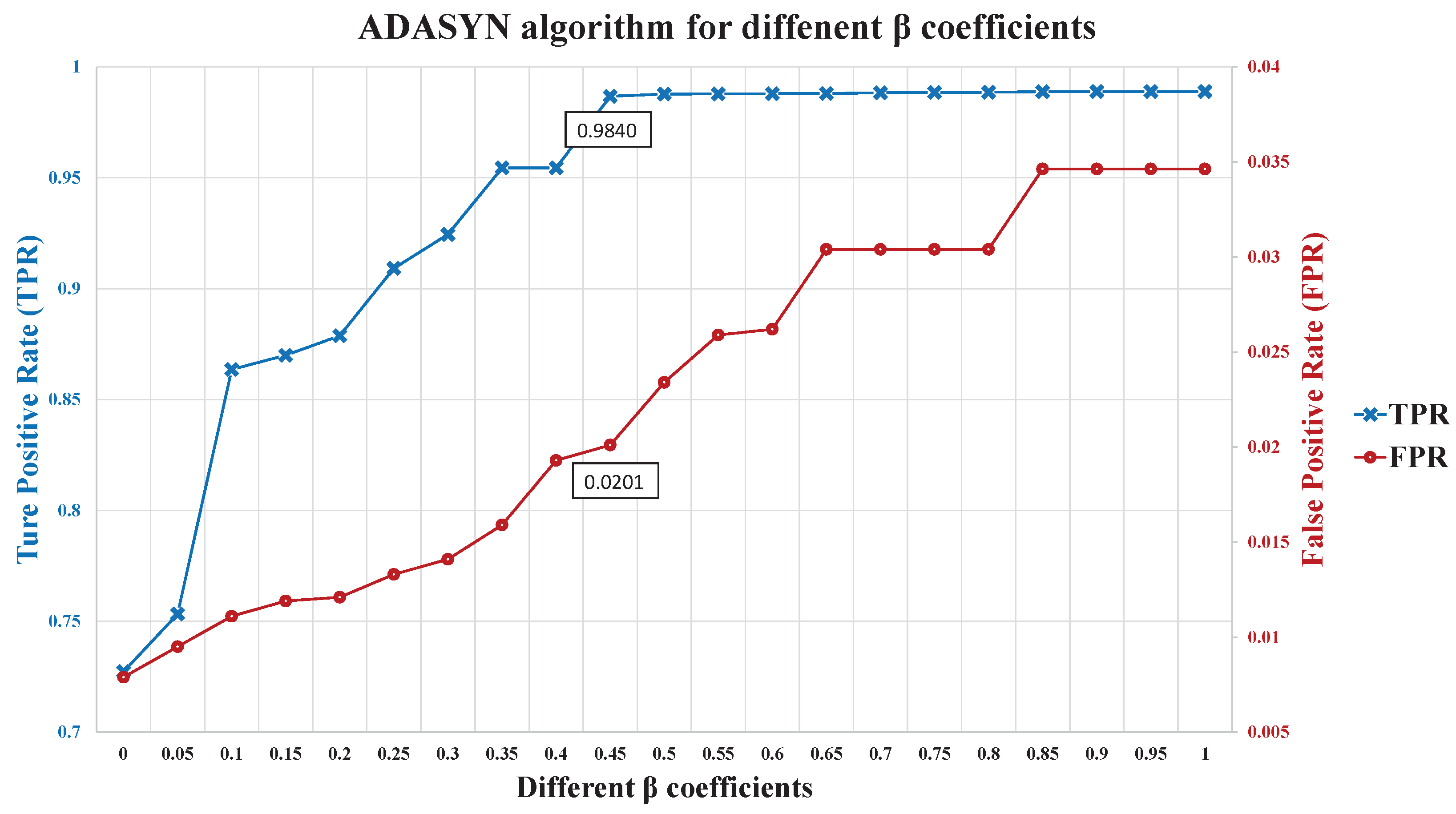
In our experiment, Figure 12 shows the evaluation results of the ADASYN algorithm for different levels. When was greater than 0.45, the TPR was more than 0.98. Therefore, the balance coefficient was selected. Table 4 shows the number of new synthetic samples. Majority represents the size of the stable class and Minority represents the size of the unstable class.
The evaluation results of the event-class predictor are shown in Table 5. There were 10 sets of testing samples. The average ACC was 97.94%, the average TPR was 98.40%, and the average FPR was 2.01%. Due to the high accuracy of event-class predictor, it can be used to choose a decision to switch between the models of different data patterns.
Table 6 shows comparisons of the event-class predictor with other common classifiers, such as BPNN, Support Vector Machine (SVM), and Adaboost. The ACC of all classifiers were greater than 90%. A good classifier needs to have high TPR and low FPR. Although the FPR of our classifier, compared with BPNN and Adaboost, was a little higher, the TPR of our proposed classifier was much higher than that of the others. This means that our classifier exhibited a higher ratio of correct classification.
5.3. Evaluation of Model Switched Landslide Prediction System
In the following experiments, the same datasets as used in Section 5.1 were employed to evaluate our landslide prediction model. To evaluate the proposed MoSLaPS model, several performance indicators were used and defined as follows:
- Mean Absolute Percent Error (MAPE) is defined as in Equation (26), where n is the number of predicted data, is the actual value, and is the predicted value.
- Root Mean Squared Error (RMSE) is defined as in Equation (27), where n is the number of predicted data samples, is the actual FS value, and is the predicted FS value.
- Normalized Root Mean Squared Error (NRMSE) is defined as in Equation (28), where is the mean of the actual values.
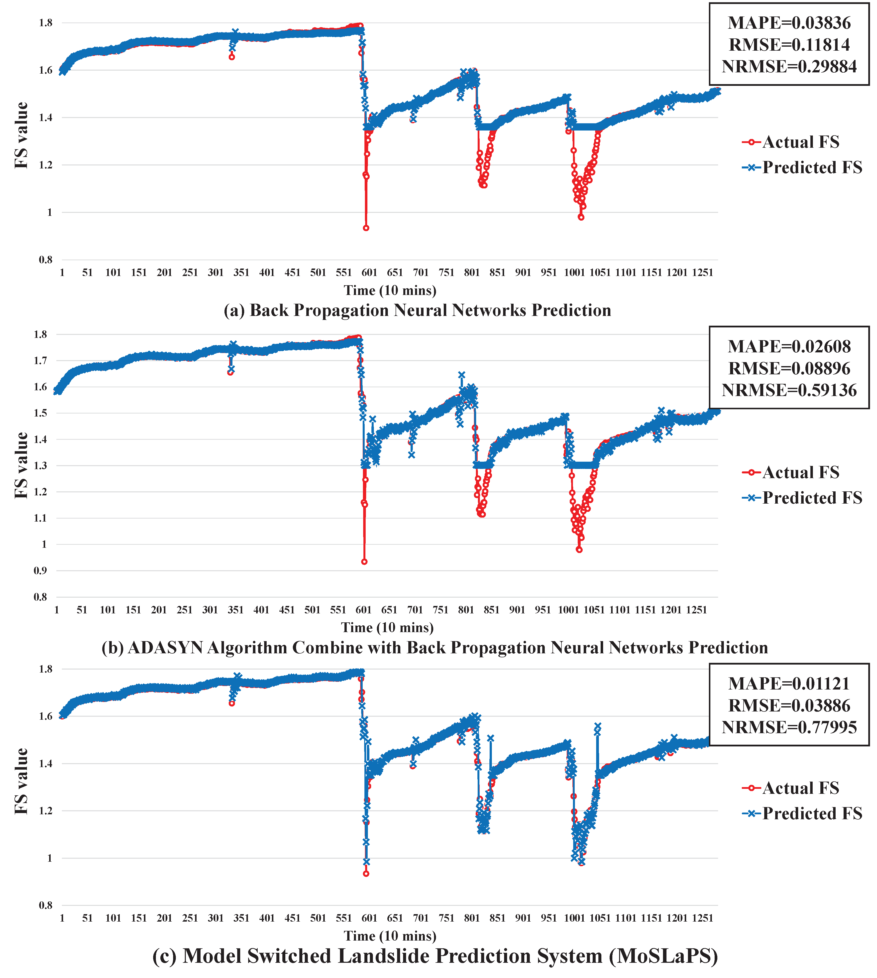
Figure 13 shows the actual FS and predicted FS for every 10 min. A BPNN prediction model is not able to learn the pattern of unstable class, as the size of the unstable class is much smaller than that of the stable class. If the original past data were used, the BPNN was not able to predict landslide occurrences. However, after processing the training data using the ADASYN algorithm to re-balance the distribution of classes, a single BPNN prediction model was still not able to learn the pattern of unstable class perfectly. This is because the data of the stable and unstable classes affected each other. As a solution, two BPNN prediction models Were proposed, one to learn the pattern of the stable class and another to learn the pattern of the unstable class. To switch between two BPNN models, an event-class predictor was constructed that can deal with imbalanced data distribution to predict the future class as a decision. Therefore, our proposed MoSLaPS method could learn the patterns of both the stable and unstable classes.
We compared our proposed MoSLaPS method with the above-mentioned methods, including a single BPNN and ADASYN+BPNN. A single BPNN was described, in detail, in Section 3.1; and ADASYN+BPNN use the ADASYN algorithm to re-balance the training data. After re-balancing, the processed training data were applied to train the BPNN.
The error metrics were evaluated for MoSLaPS, ADASYN+BPNN, and BPNN. Compared with BPNN and ADASYN + BPNN, our method resulted in much smaller MAPE and RMSE. This means that the prediction accuracy of our method was higher. The NRMSE of our method was also larger than that of the others, which means that our prediction results were closer to the real situation.
Although MoSLaPS was more accurate than the other methods, it requires a little more computation time and resources. As shown in Table 7, the simulation results of the different methods shows that the speed of MoSLaPS was a little slower than that of BPNN and ADASYN+BPNN, and its CPU and memory usages were higher than the others. This is because MoSLaPS took extra computational time and resources to deal with the imbalanced data classification and switching between the different predictors. In our experiment, the time interval was 10 mins; so there was ample time to deal with the process.
5.4. Evaluation of Landslide Pre-Alarm
The same datasets as in Section 5.1 were applied to evaluate our landslide pre-alarm method. Table 8 shows the prediction time (PT) for ten different experiments. For each experiment, the minimum PT, maximum PT, and average PT were recorded. From Table 8, the program was able to observe that the prediction time for dataset was the longest (52.2 min); while that for dataset was the shortest (38.4 min). As a shorter prediction time indicates that the change of FS is intense and quick, dataset represented a higher probability of landslide occurrence. Taking the average of all timings, it can be seen that the proposed MoSLaPS method could warn of the occurrence of a landslide an average of 44.2 min in advance.
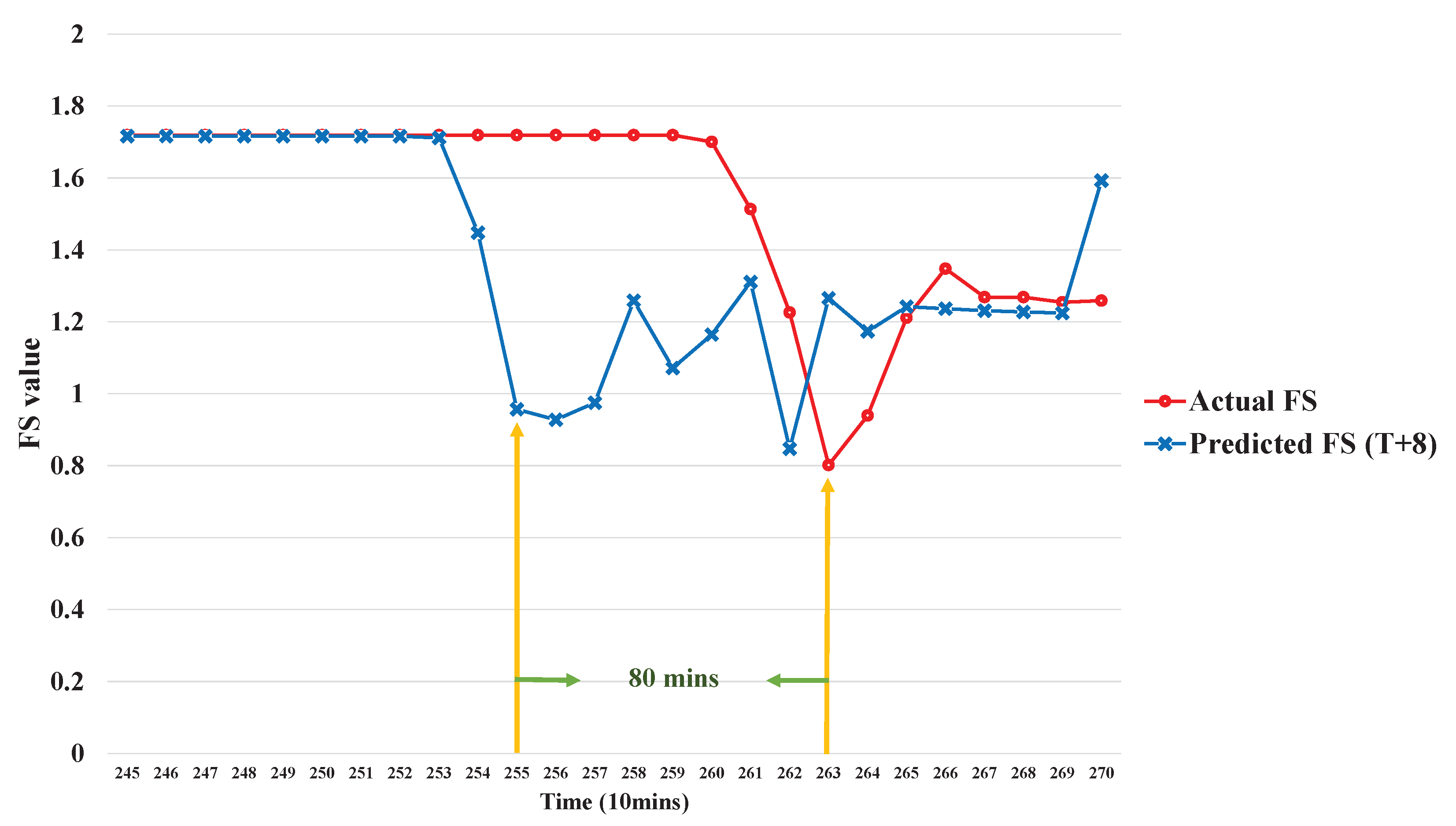
Further, we take a best-case example, to demonstrate how the proposed method can warn of landslide occurrence far in advance. At time point 255, the 8th prediction result is ; that is, a landslide will occur after eight time units, as shown in Figure 14. In our experiments, the interval between two time points is 10 min. Hence, the landslide occurrence could be predicted and warned about 80 min in advance.
6. Conclusions
To address the problems of imbalanced data, low true positive rate for learning, determining the prediction horizon, and the time for model re-training, MoSLaPS has been proposed as a novel method for landslide prediction. MoSLaPS employs the ADASYN method to balance the stable class (no landslide) with the unstable class (landslide), where the classification is based on the factor of safety calculated using the SHALSTAB model. To solve the problem of low true positive rate, a BPNN-based event-class predictor was proposed and two BPNN predictors were designed to learn the stable class pattern and the unstable class pattern. A novel prediction horizon tuning method was proposed, along with a learning-based model re-training technique. All of these optimizations contribute towards the goal of the proposed MoSLaPS; that is, accurate early warning of landslides.
Compared with BPNN and Adaboost, though our event-class predictor has a higher FPR, it also has a much higher TPR of 98.40%. This means our classifier has a higher ratio of correct classification. According to the predicted class, our system can switch between different predictors to adapt to the environmental state. In addition, BPNN is employed to construct the error model to predict the future errors of our proposed MoSLaPS and compensate for these errors in the prediction phase. As a result, MoSLaPS has much lower MAPE and RMSE than BPNN and ADASYN+BPNN, which means that MoSLaPS is more accurate. In addition, the NRMSE of our method is larger than the NRMSE of the other methods, which means that our method is closer to the actual conditions. Statistically, our landslide prediction system could send warnings an average of 44.2 min prior to the actual occurrence of a landslide.
In the future, we will further consider other advanced imbalanced learning algorithms to improve the performance of BPNN-based event-class predictors. For different applications, a larger number of categories (cases) can be considered for model switching. The maximum range of errors allowed in the re-training phase can also be limited, so that prediction models are more stable. As a result, the model switching strategy will be more accurate. Moreover, well-known time-series deep learning technologies, such as Recurrent Neural Networks (RNNs) or Long-Short Term Memory (LSTM) blocks, will be used to combine all three BPNN models into one.
Author Contributions
Conceptualization, P.-A.H.; methodology, D.U.; software, S.-F.C.; validation, S.-F.C. and D.U.; resources, P.-A.H.; data curation, S.-F.C.; writing—original draft preparation, S.-F.C.; writing—review and editing, D.U.; supervision, P.-A.H.; project administration, P.-A.H.; funding acquisition, P.-A.H.
Funding
This research was funded by Ministry of Science and Technology, Taiwan, grant number MOST 140-2221-E-194-064.
Acknowledgments
This research was supported partially by the project grant MOST-107-2221-E-194-001-MY3 from the Ministry of Science and Technology, Taiwan.
Conflicts of Interest
The authors declare no conflict of interest.
Abbreviations
The following abbreviations are used in this manuscript:
| ANN | Artificial Neural Network |
| WSN | Wireless Sensor Network |
| FS | Factor of Safety |
| MoSLaPS | Model Switched Landslide Prediction System |
| LMA | Levenberg–Marquardt algorithm |
| ADASYN | Adaptive Synthetic Sampling |
| SMOTE | Synthetic Minority Oversampling Technique |
| EEW | Error Estimation Window |
| PH | Prediction Horizon |
| TPR | True Positive Rate |
| FPR | False Positive Rate |
| ACC | Accuracy |
| TP | True Positive |
| TN | True Negative |
| FP | False Positive |
| FN | False Negative |
| MAPE | Mean Absolute Percentage Error |
| RMSE | Root Mean Squared Error |
| NRMSE | Normalized Root Mean Squared Error |
| PT | Prediction Time |
References
- He, H.; Bai, Y.; Garcia, E.A.; Li, S. ADASYN: Adaptive synthetic sampling approach for imbalanced learning. In Proceedings of the IEEE International Joint Conference on Neural Networks (IEEE World Congress on Computational Intelligence), Hong Kong, China, 1–8 June 2008; pp. 1322–1328. [Google Scholar]
- Jiang, T.; Wand, D. A landslide stability calculation method based on Bayesian network. In Proceedings of the Instrumentation and Measurement, Sensor Network and Automation, Toronto, ON, Canada, 23–24 December 2013; pp. 905–908. [Google Scholar]
- Devi, S.R.; Venkatesh, C.; Agarwa, P.; Arulmozhivarman, P. Daily rainfall forecasting using artificial neural networks for early warning of landslides. In Proceedings of the International Conference on Advances in Computing, Communications and Informatics, New Delhi, India, 24–27 September 2014; pp. 2218–2224. [Google Scholar]
- Kavzoglu, T.; Sahin, E.K.; Colkesen, I. Selecting optimal conditioning factors in shallow translational landslide susceptibility mapping using genetic algorithm. Eng. Geol. 2015, 192, 101–112. [Google Scholar] [CrossRef]
- Huang, J.C.; Kao, S.J.; Hsu, M.L.; Liu, Y.A. Influence of specific contributing area algorithms on slope failure prediction in landslide modeling. Nat. Hazards Earth Syst. Sci. 2007, 7, 781–792. [Google Scholar] [CrossRef]
- Popescu, M. A suggested method for reporting landslide remedial measures. Bull. Eng. Geol. Environ. 2001, 60, 69–74. [Google Scholar] [CrossRef]
- Lian, C.; Zeng, Z.; Yao, W.; Tang, H. Multiple neural networks switched prediction for landslide displacement. Eng. Geol. 2015, 186, 91–99. [Google Scholar] [CrossRef]
- Lian, C.; Chen, C.L.P.; Zeng, Z.; Yao, W.; Tang, H. Prediction Intervals for Landslide Displacement Based on Switched Neural Networks. IEEE Trans. Reliab. 2016, 65, 1483–1495. [Google Scholar] [CrossRef]
- Huang, J.C.; Kao, S.J. Optimal estimator for assessing landslide model performance. Hydrol. Earth Syst. Sci. 2006, 10, 957–965. [Google Scholar] [CrossRef]
- Hagan, M.T.; Demuth, H.B.; Beale, M.H.; De Jesús, O. Neural Network Design. 2014. Available online: http://hagan.okstate.edu/NNDesign.pdf (accessed on 3 May 2019).
- Levenberg Marquardt Algorithm. 2017. Available online: https://en.wikipedia.org/w/index.php?title=Levenberg%E2%80%93Marquardt_algorithm&oldid=771936514 (accessed on 3 May 2019).
- Jacobian Matrix and Determinant. 2017. Available online: https://en.wikipedia.org/w/index.php?title=Jacobian_matrix_and_determinant&oldid=776906112 (accessed on 3 May 2019).
- Palit, A.K.; Popovic, D. Computational Intelligence in Time Series Forecasting: Theory and Engineering Applications; Springer Science & Business Media: London, UK, 2006. [Google Scholar]
- Ertekin, S.; Huang, J.; Bottou, L.; Giles, L. Learning on the border: active learning in imbalanced data classification. In Proceedings of the 16th ACM Conference on Conference on Information and Knowledge Management, Lisbon, Portugal, 6–10 November 2007; pp. 127–136. [Google Scholar]
- Chawla, N.V.; Bowyer, K.W.; Hall, L.O.; Kegelmeyer, W.P. SMOTE: Synthetic minority over-sampling technique. J. Artif. Intell. Res. 2002, 16, 321–357. [Google Scholar] [CrossRef]
- Soil and Water Conservation Bureau Platform for Monitoring Data. 2016. Available online: http://monitor.swcb.gov.tw (accessed on 3 May 2019).
Figure 1.
Model switched landslide prediction system architecture.
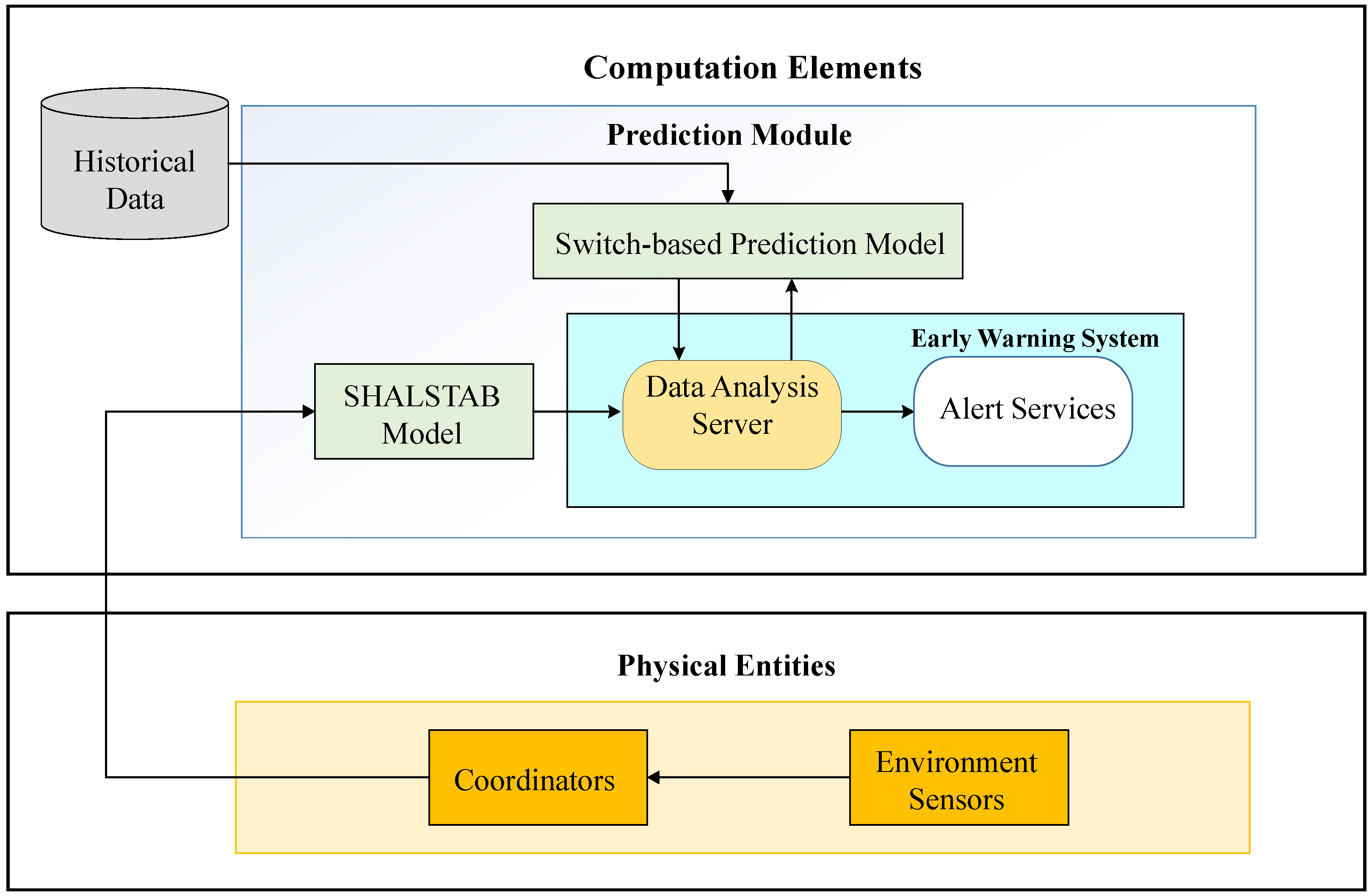
Figure 2.
Back-Propagation Neural Network (BPNN) prediction model framework design.

Figure 3.
A fully connected feed-forward Back-Propagation Neural Network with time-series.

Figure 4.
Flow of constructing the event-class predictor.

Figure 5.
Flow of constructing different pattern predictors.

Figure 6.
Flow of the switching strategy.

Figure 7.
Overall Flowchart of Prediction Model Analysis.
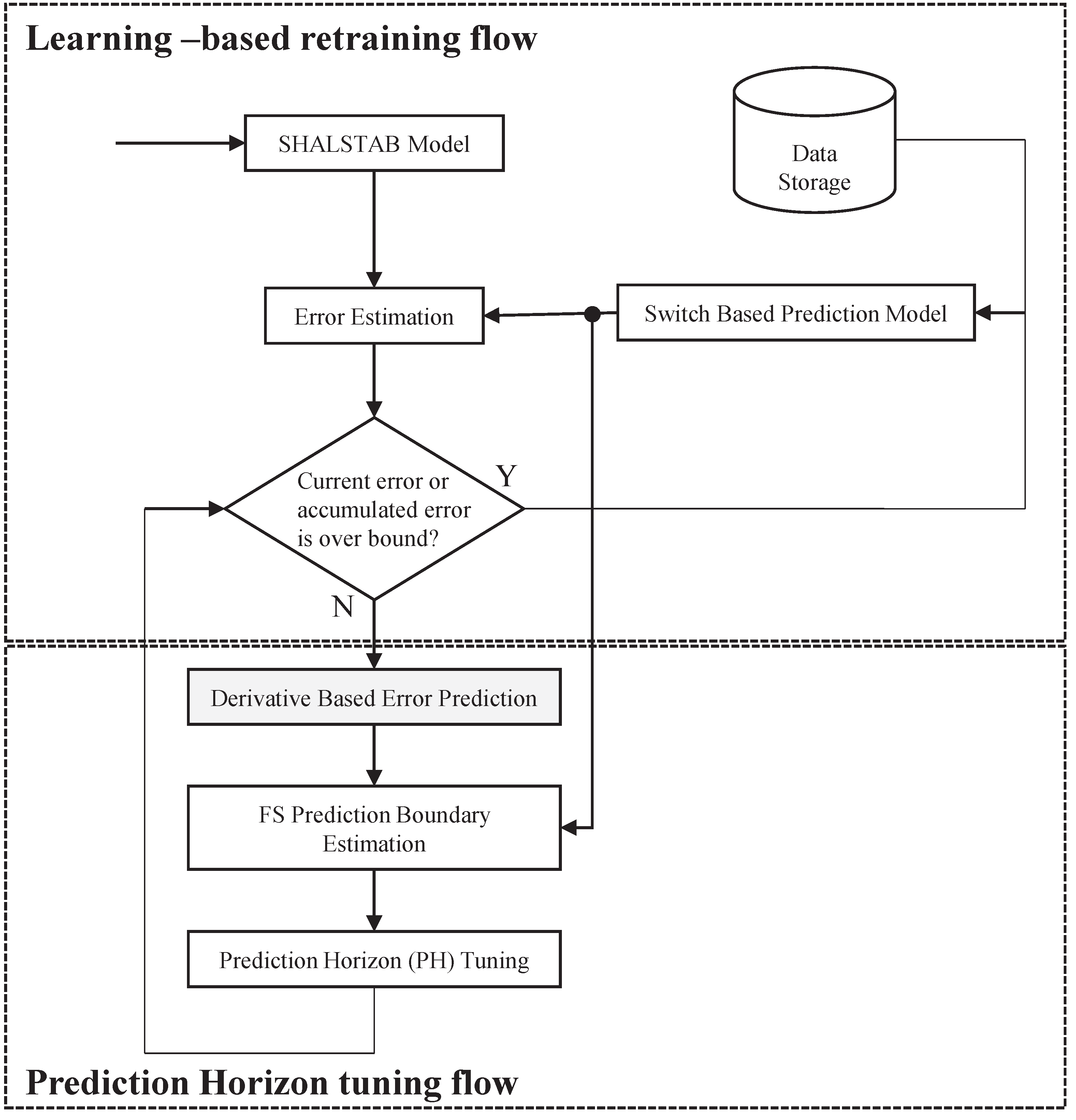
Figure 8.
Learning-based re-training flow.

Figure 9.
Prediction horizon tuning.

Figure 10.
Monitoring curves of Factor of Safety and rainfall at Shen-Mu station.

Figure 11.
Monitoring curves of Factor of Safety and soil moisture at Shen-Mu station.

Figure 12.
The evaluation result of the ADASYN algorithm for different values of the coefficient .

Figure 13.
Comparison of the proposed method with other BPNN methods.

Figure 14.
Landslide early warning time point.


Table 1.
Comparison of Landslide Detection/Prediction Methods.
| Types | Methods | Advantages | Accuracies |
|---|---|---|---|
| Image Analysis | Geographical | Suitable for | Accuracy based |
| Information System [4] | Large Area | on number of layers | |
| Machine Learning | Bayesian Network [2] | Simple Network | 75% |
| Neural Network [3] | Simple Network | 67% | |
| Genetic Algorithm [4] | Optimal Solution | 90% | |
| Mathematical Evaluation | SHALSTAB * [6] | High Accuracy | >90% |
* Shallow Landsliding Stability Model.
Table 2.
Classification of Factor of Safety (FS) Levels.
| Stable Region | FS |
| Marginally Stable Region | 1.3 > FS |
| Actively Unstable Region | FS < 1 |
Table 3.
Confusion matrix.
| Actual Class | |||
|---|---|---|---|
| Unstable | Stable | ||
| Prediction Class | Unstable | True Positive | False Positive |
| Stable | False Negative | True Negative | |
Table 4.
Number of synthetic new samples generated by the ADASYN algorithm ().
| All Dataset | Majority | Minority | ADASYN |
|---|---|---|---|
| 1300 | 1280 | 20 | 449 |
| 1300 | 1199 | 101 | 389 |
| 1300 | 1222 | 78 | 424 |
| 1300 | 1181 | 119 | 374 |
| 1300 | 1199 | 101 | 420 |
| 1300 | 1291 | 9 | 464 |
| 1300 | 1227 | 73 | 414 |
| 1300 | 1224 | 76 | 408 |
| 1300 | 1056 | 244 | 299 |
| 1300 | 1140 | 160 | 341 |
Table 5.
The evaluation results of the event-class predictor.
| No. | ACC | TPR | FPR | TP | FP | TN | FN |
|---|---|---|---|---|---|---|---|
| 1 | 96.43% | 100.00% | 3.60% | 2 | 9 | 241 | 0 |
| 2 | 97.62% | 94.44% | 2.14% | 17 | 5 | 229 | 1 |
| 3 | 98.41% | 95.45% | 1.30% | 21 | 3 | 227 | 1 |
| 4 | 98.41% | 100.00% | 1.64% | 8 | 4 | 240 | 0 |
| 5 | 96.03% | 100.00% | 3.98% | 1 | 10 | 241 | 0 |
| 6 | 100.00% | 100.00% | 0.00% | 16 | 0 | 236 | 0 |
| 7 | 96.03% | 100.00% | 4.03% | 4 | 10 | 238 | 0 |
| 8 | 99.21% | 100.00% | 0.83% | 12 | 2 | 238 | 0 |
| 9 | 98.41% | 100.00% | 1.68% | 14 | 4 | 234 | 0 |
| 10 | 98.81% | 94.12% | 0.85% | 16 | 2 | 233 | 1 |
| Average | 97.94% | 98.40% | 2.01% | ||||
Table 6.
Comparison of event-class predictor with other common classifiers.
| Method | ACC | TPR | FPR |
|---|---|---|---|
| Event-Class | 97.94% | 98.40% | 2.01% |
| BPNN | 97.16% | 57% | 0.42% |
| SVM | 90.42% | 78.06% | 9.02% |
| Adaboost | 98.27% | 75.1% | 0.96% |
Table 7.
Comparisons of time consumption and resource usage.
| Method | Time (s) | CPU Usage | Memory |
|---|---|---|---|
| MoSLaPS | 1.205 | 23.90% | 972 kb |
| ADASYN+BPNN | 0.739 | 20.30% | 192 kb |
| BPNN | 0.639 | 19.90% | 148 kb |
Table 8.
Prediction time in advance for different datasets.
| No. | Min. PT (min) | Max. PT (min) | Avg. PT (min) |
|---|---|---|---|
| 1 | 10 | 80 | 40 |
| 2 | 10 | 70 | 33.3 |
| 3 | 10 | 50 | 35.7 |
| 4 | 20 | 80 | 47.6 |
| 5 | 10 | 80 | 52.2 |
| 6 | 10 | 80 | 51.8 |
| 7 | 10 | 80 | 42.6 |
| 8 | 10 | 70 | 45.7 |
| 9 | 10 | 80 | 43.3 |
| 10 | 10 | 80 | 38.4 |
| Avg. | 10.7 | 76.4 | 44.2 |
© 2019 by the authors. Licensee MDPI, Basel, Switzerland. This article is an open access article distributed under the terms and conditions of the Creative Commons Attribution (CC BY) license (http://creativecommons.org/licenses/by/4.0/).
Share and Cite
MDPI and ACS Style
Utomo, D.; Chen, S.-F.; Hsiung, P.-A. Landslide Prediction with Model Switching. Appl. Sci. 2019, 9, 1839. https://doi.org/10.3390/app9091839
AMA Style
Utomo D, Chen S-F, Hsiung P-A. Landslide Prediction with Model Switching. Applied Sciences. 2019; 9(9):1839. https://doi.org/10.3390/app9091839
Chicago/Turabian StyleUtomo, Darmawan, Shi-Feng Chen, and Pao-Ann Hsiung. 2019. "Landslide Prediction with Model Switching" Applied Sciences 9, no. 9: 1839. https://doi.org/10.3390/app9091839
Note that from the first issue of 2016, this journal uses article numbers instead of page numbers. See further details here.