Vibration-Based Bearing Fault Detection and Diagnosis via Image Recognition Technique Under Constant and Variable Speed Conditions

Featured Application

The proposed technique can be applied in different industrial applications and it is expected to be applied to the End-of-Line (EoL) quality control of gearboxes production lines and as a condition-monitoring tool for operational conditions of machines working in variable speed condition as wind turbines or bearings of train and cars.

Abstract

This paper addresses the application of an image recognition technique for the detection and diagnosis of ball bearing faults in rotating electrical machines (REMs). The conventional bearing fault detection and diagnosis (BFDD) methods rely on extracting different features from either waveforms or spectra of vibration signals to detect and diagnose bearing faults. In this paper, a novel vibration-based BFDD via a probability plot (ProbPlot) image recognition technique under constant and variable speed conditions is proposed. The proposed technique is based on the absolute value principal component analysis (AVPCA), namely, ProbPlot via image recognition using the AVPCA (ProbPlot via IR-AVPCA) technique. A comparison of the features (images) obtained: (1) directly in the time domain from the original raw data of the vibration signals; (2) by capturing the Fast Fourier Transformation (FFT) of the vibration signals; or (3) by generating the probability plot (ProbPlot) of the vibration signals as proposed in this paper, is considered. A set of realistic bearing faults (i.e., outer-race fault, inner-race fault, and balls fault) are experimentally considered to evaluate the performance and effectiveness of the proposed ProbPlot via the IR-AVPCA method.

1. Introduction

Detecting and diagnosing the different faults in modern engineered systems is crucial to designing a better condition monitoring strategy for preventing the degradation from early stage simple faults into serious or even catastrophic system failures. In the fault detection and diagnosis (FDD) field, two main groups of the applied approaches exist. Model-based FDD approaches [1] that are based on developing a reference model or observer—using mathematics or physics law—are used to generate residual vectors, which describe the system health state to detect and isolate faults if a deviation from the expected values is observed. Those methods are very powerful FDD methods if an accurate reference model/observer can be achieved, which is itself a nontrivial problem [2]. Further, both output and input signals of the system are needed for modeling, in which the latter are not always available, especially for a part of the system, e.g., the bearing inside the rotating electrical machines (REMs). Thus, the established analytical model is often unrealistic and not accurate enough to be a reference due to the complexity of those modern engineered systems. Therefore, the data-driven approaches, which are model-free techniques and often do not need real system input information, but only a bunch of output data (historical data), are considered as alternative solutions to deal with bearing fault detection and diagnosis (BFDD).

Different existing data-driven-based BFDD techniques use data acquisition equipment and measurements, such as vibrations; chemical, temperature, and acoustic emissions; sound pressure; stator current monitoring [3]; and rotor speed analysis [4]. In particular, recent surveys [5,6,7,8] indicate a clear tendency toward the vibration monitoring of REMs. These methods usually require the extraction of a set of features from the aforementioned raw signals in order to classify the bearing faults [9]. For extracting useful features, usually the acquired signals are processed using Fourier transform (FT) or its variants (i.e., fast FT (FFT), discrete FT (DFF)) [10], wavelet transform (WT) or its variants (i.e., continuous WT (CWT), discrete WT (DWT), wavelet packet transform (WPT)) [11,12], envelope analysis [13,14], or statistical methods (e.g., principal component analysis (PCA), linear discriminant analysis (LDA)) [15,16,17,18,19]. Thus, the extracted features could be in time domain, frequency domain, or time-frequency domain, which usually have physical meanings, or purely statistical features, which usually do not have physical meanings [20,21]. However, these features are generally in the form of a vector or scalar, for which they have some descriptions of the waveform in the time domain and some parameters of the spectrum in the frequency domain, or just a statistical vector index.

Therefore, a single feature only describes one aspect of the vibration signals. Thus, many works combine more than one feature to improve the performance of bearing fault detection and diagnosis using different techniques to make full use of multi-features in time domain, frequency domain, time-frequency domain, or the purely statistical domain [22,23]. However, combining multiple features using fusion techniques may increase the complexity of the used methods, and mostly the results cannot be interpreted, in addition to the appearance of key issues of feature extraction, i.e., the high dimensionality of feature space and the large number of features. Thus, a dimensionality reduction technique and a single feature that can include rich information about the system’s health conditions should be considered. Therefore, this paper uses an image, which is known as the best way that includes rich information for the efficient recognition and classification of different objects [24], and a modified PCA-based technique, which is one of the most used techniques for dimensional reduction, for vibration-based BFDD under constant and variable speed conditions (i.e., non-stationary conditions).

One has to consider the above-mentioned issues when using a single time domain, frequency domain, or time-frequency domain feature that represents only some characteristics of the vibration signals, or fusing multiples features that boost the processing method complexity, the dimensionality of the feature space, and the number of the extracted features. In addition, some researchers used contemporary methods (i.e., shallow learning or deep learning) as (or and) image-processing algorithm to detect and diagnose bearing faults [25,26,27,28], which are different from using image recognition methods [24], as proposed in this paper, which do not require a processing phase (less time-consuming). This paper thus proposed a novel BFDD technique that uses the ProbPlot to generate features in the form of images and then an image recognition technique based on the AVPCA [4], namely, the ProbPlot via IR-AVPCA technique, to detect and diagnose the different bearing faults under constant and variable speed conditions.

This paper novelty is about using for the first time the ProbPlot to generate the features (images) directly from the raw vibration signals under different operating conditions (i.e., healthy and faulty) to be the inputs for the AVPCA algorithm that is used as a shape recognition tool for detecting present of faults (i.e., under bearing fault free (BFF) case) and diagnosing different bearing faults (i.e., outer-race fault (ORF), inner-race fault (IRF), and ball bearing fault (BBF)). On the contrary, in the previous paper [4], the authors developed the AVPCA algorithm and used it as a feature extraction and then for classification to detect and diagnose the different bearing faults using only the rotor-speed signal. Furthermore, the PCA method was used for the condition monitoring systems (CMSs) [29,30,31] and for bearing fault detection and diagnosis [4,17,32,33]. However, it was never used as an image recognition tool to BFDD as proposed in this paper. It was only used as an image processing method as in [23], but they used the FFT to create the images (the features) and the two-dimensional PCA to reduce the dimensions, and then a minimum distance method was applied to classify the faults of bearings. On the contrary, the proposed paper uses the ProbPlot to generate the features (images) and the AVPCA algorithm for bearing fault detection and diagnosis, which has never been used before.

This paper is organized as follows. The proposed ProbPlot via IR-AVPCA technique for bearing fault detection and diagnosis is described in Section 2. The experimental results of the vibration-based ball bearing fault detection and diagnosis are presented in Section 3, and the conclusion is drawn in Section 4.

2. The ProbPlot via IR-AVPCA Technique for Bearing Fault Detection and Diagnosis (BFDD)

The use of an image recognition technique in the field of BFDD requires only the generation of the features as images to be the inputs (database) of this image recognition technique. Thus, no feature extraction phase is needed; instead, only a feature (image) generation phase is required, which is less complex than the former. Many possible choices exist for generating the vibration signal features in the form of images to BFDD: (i) the features (images) can be obtained directly in time domain from the original raw data of the vibration signals under the different bearing health conditions; (ii) they can be obtained in frequency domain by, for example, capturing the FFT of the vibration signals as in [23]; and (iii) or they can be obtained by generating the ProbPlot of the vibration signals as proposed for the first time in this paper, which has the advantage of not needing computation or analysis compared, unlike the FFT-based method. Further, contrary to the limitation of using the FFT to generate the features (images) for BFDD, since it is only suitable under steady state conditions but not under nonstationary conditions (i.e., variable speed, current, and/or torque), because the information about time will be lost [34], the proposed ProbPlot-based method can deal with the nonstationary conditions, which are more realistic work conditions, especially when dealing with bearings. A detailed description of the proposed ProbPlot via IR-AVPCA technique to BFDD is given below.

2.1. ProbPlot of the Vibration Signals and Features Creation Tool

By definition, the probability plot [35] is a “graphical technique for assessing whether or not a data set follows a given distribution, such as the normal or Weibull”; this paper considers the normal probability plot due to its importance in many statistical applications [36]. The ProbPlot strategy plots the vibration raw data according to a theoretical distribution (i.e., normal or Weibull) so that the resulted points should be bordered and form a straight line. Any deviation from this bordered straight line indicates a deviation from the current specified distribution, since the correlation coefficient (of the ProbPlot) associated with the linear fit of the considered raw data is a measure of the fit itself. Thus, using this merit, the different bearing fault can be detected and then diagnosed, in which the further the ProbPlot results vary from the straight line, the greater the detection and the diagnosis of the bearing faults that is achieved.

For generating the best features (images), the highest correlation coefficient must be chosen, since it will generate the straightest probability plot. The features (images) created through the ProbPlot will be formed by a vertical axis, which comprises ordered response values, and horizontal axis, which comprises order statistic medians for the given distribution. These order statistic medians, Me_i, can be approximated by [37]:

$$M{e}_i=f\left(M{u}_i\right)$$

(1)

in which f is the percent point function for the desired distribution, which is the inverse of the cumulative distribution function, and Mu_i are the uniform order statistic medians defined as [37]:

$$\{\begin{array}{c}M{u}_i=1-M{u}_i for i=1\\ M{u}_i=\frac{\left(i-0.3175\right)}{\left(n+0.365\right)} for i=2,3,\cdots ,n-1\\ M{u}_i={0.5}^{\left(\raisebox{1ex}{$1$}\!\left/ \!\raisebox{-1ex}{$n$}\right.\right)} for i=n\end{array}$$

(2)

One advantage of the proposed ProbPlot-based features generation in the form of images (as proposed in this paper) is that it is very easy; further, it is a straightforward method, and the results can be directly interpreted.

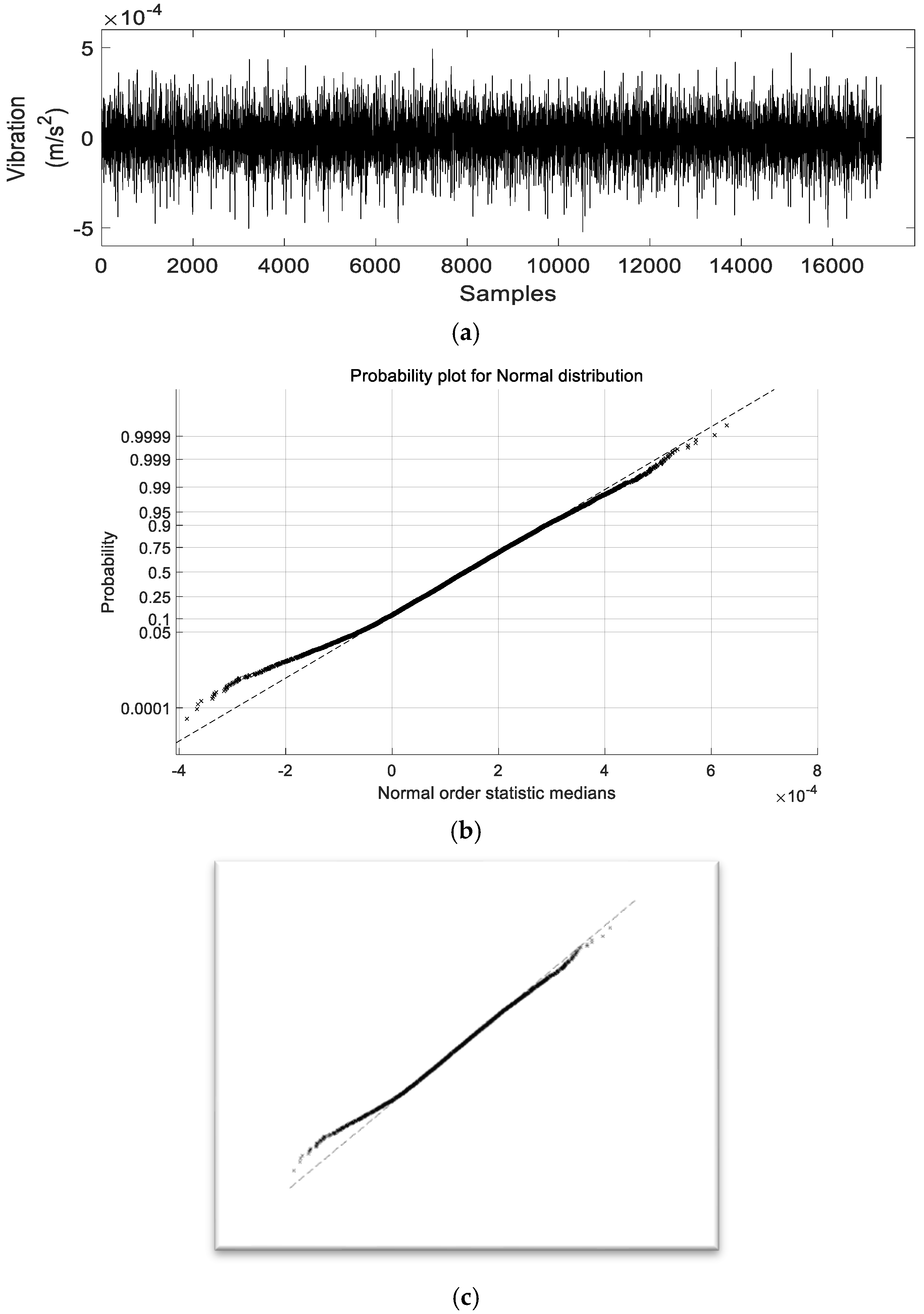
In order to generate the features (images), both x-axis and y-axis are auto-scaled when capturing the image so the only parameter of the image (feature) is the size in pixels. Then, all irrelevant information, such the axis, the titles, labels, and so on, were eliminated, and the only pure ProbPlots of the vibration signals were captured to form the features, as can be seen in Figure 1.

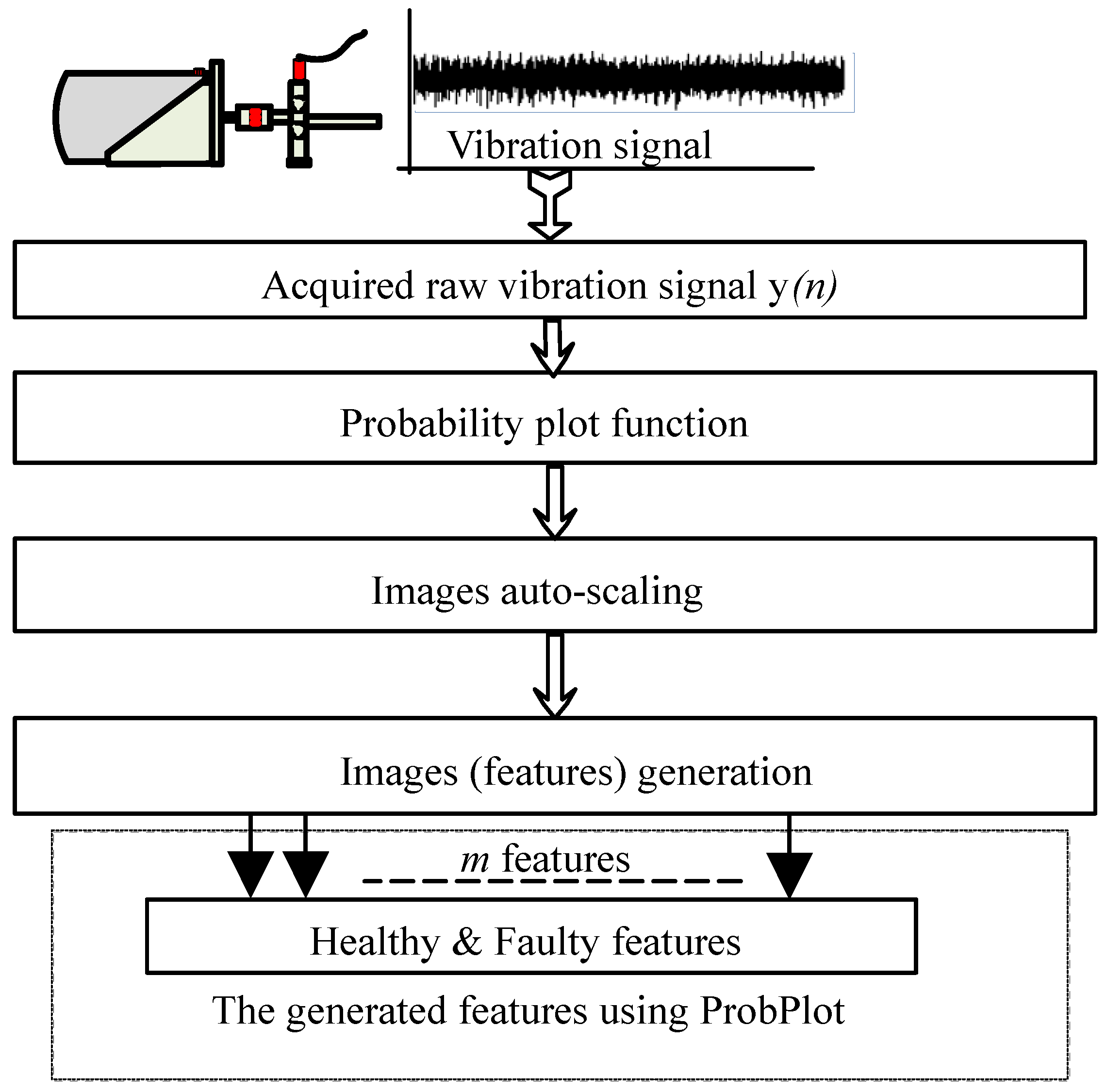
The flowchart of the ProbPlot-based features generation in Matlab is shown in Figure 2. Note that m is the number of all possible faulty cases and the fault-free case, which are known as clusters. In our application,

• m = 1 for the BFF cluster,
• m = 2 for the ORF cluster,
• m = 3 for the IRF cluster, and
• m = 4 for the BBF cluster.

2.2. AVPCA-Base Image Recognition

PCA is a linear transformation commonly used for compressing redundant data and recently successfully applied for image processing and classification [38]. In the following, a description of the PCA-based image recognition and a fault recognition process followed by the AVPCA-based BFDD will be given.

2.2.1. PCA to image recognition

PCA algorithm is a method that aims to best present the data by projection (in a least square sense) for reducing the dimension and compressing the data. In image analysis, the PCA takes the 2-D image and represents it as a 1-D image vector by liaising each row/column into a long vector. Thus, the image vectors x_i are defined as [39]:

$$x_i={\left[{\sigma }_1,\cdots ,{\sigma }_N\right]}^T;i=1\cdots M$$

(3)

in which M is the number of vectors that represent the sampled image, which are of size N, and σ_j’s represents the pixel. Subtracting the mean image mi from each image vector, the mean centered c_i of the image is computed as:

$$c_i=x_i-mi$$

(4)

in which

$$mi=\frac{1}{M}{\displaystyle \sum }_{i=1}^M{x}_i$$

(5)

Maximizing the quantity in which

$${\lambda }_i=\frac{1}{M}{\displaystyle \sum }_{n=1}^M{\left(v_i^T{C}_n\right)}^2$$

(6)

with the orthonormality constraint $v_i^T{v}_k={\delta }_{ik}$ allows the finding of a set of M orthogonal vectors v_i’s, which have the largest possible projection onto each of the c_i’s. v_i’s and λ_i’s are the eigenvectors and eigenvalues, respectively, of the covariance matrix W_nxn that is defined as

$$W=C{C}^{\mathrm{T}}$$

(7)

in which C is a matrix in which its columns are the vectors c_i placed side by side.

In practice, it is not a suitable solution to find the v_i and λ_i of the covariance matrix W. Thus, in linear algebra, the calculation of the eigenvectors v_i and eigenvalues λ_i is obtained by finding those of the C^TC matrix of size M × M, i.e., finding e_i and µ_i, the eigenvectors and eigenvalues of C^TC, respectively, in which

$$C{C}^T{e}_i={\mu }_i{e}_i$$

(8)

If both sides of Equation 8 are multiplied by C: $C{C}^T(C{e}_i)={\mu }_i\left(C{e}_i\right)$, then, the first M − 1 eigenvectors v_i and eigenvalues λ_i of matrix CC^T correspond to Ce_i and µ_i, respectively. However, first, the rank of the covariance matrix should not exceed M−1, and the eigenvectors Ce_i have to be normalized to be equal to v_i. Therefore, the computed eigenvectors will generate an orthonormal basis of the subspace that allows the representation of the image and most of its data with a minimum error. Usually, these computed eigenvectors range from the largest to the smallest following their corresponding eigenvalues, in which the largest eigenvector (corresponding to the biggest eigenvalue) reflects the greatest variance in the image and vice versa. It is found that the first 5% to 10% of the dimensions usually contain 90% of the total variance. The facial image $\Psi$ can be projected onto M’ (<<M) dimensions by calculating

$$\Psi ={\left[p_1{p}_2\cdots p_M\right]}^T;p_i=e_i^T{c}_i$$

(9)

in which p_i is the ith coordinate of the facial image $\Psi$ in the new space, which comes to be the principal component. The vectors e_i represent and are known as the eigenfaces. Fault presence recognition is achieved by minimizing the error distance.

2.2.2. Fault Recognition

For fault recognition, the AVPCA [4] is used to project the ProbPlot features (images) generated from the collected vibration signals under healthy and faulty conditions in both constant and variable speed environments. First, it generates the training bases of the space (i.e., training vectors), which correspond to the eigenvectors, which are ordered according to the largest variance of the generated ProbPlot images, in which they are described by its eigenface coefficients called the weights.

In features (images) recognition, after generating the features and computing the eigenfaces, different decisions can be achieved according to the desired target of the different applications. Consequently, the recognition can be the obtaining of the labels of individuals, i.e., the identification can be about deciding if the person has already been seen or not, i.e., the recognition of individuals; finally, the task of the recognition can be about assigning a face or a fault to a certain class, which is known as categorization.

Only the task of categorization is considered in this paper, in which the features in the training set are projected into the face space and stored in memory as AVPCA bases to form the training databases that contain the Healthy base vector H_b¹ and the Faulty base matrix F_b^m−1. Once a new feature (image) is presented as an unknown input to our system, it will be projected onto the face space and generate the test database that contain the Data-test vector T_b^new. Then, our proposed algorithm computes its error distance from all stored training databases. The smallest distance gives the desired class. This information is used to detect the presence or absence of the fault and then diagnose the different bearing faults (ORF, IRF, and BBF).

2.2.3. Absolute Value Principal Component Analysis (AVPCA) for Bearing Fault Detection and Diagnosis

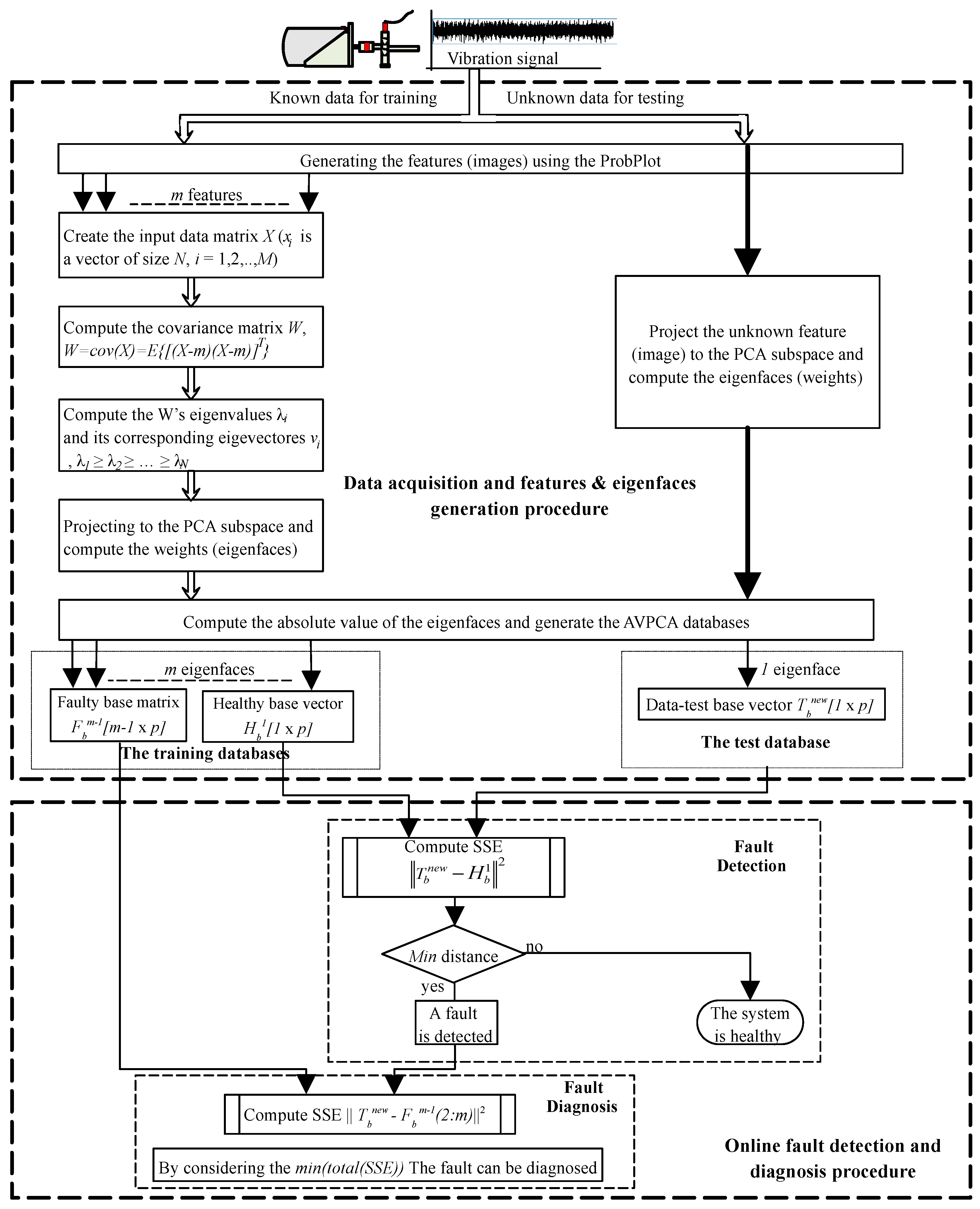
In this paper, to make the proposed vibration-based BFDD via image recognition more suitable for online condition monitoring, we used AVPCA, which is an improved version of the classical PCA but with no mathematical complications simply by taking the absolute value of the weights to generate the bases, and the use of the sum of squared error (SSE) distances [4]. Furthermore, the probability plot parameters (the intercept and slope) will vary with the presence of the different bearing faults, but differently. Since the effect of the presence of the bearing faults causes variations of the faulty parameters that comprise particular information related to the fault itself, the considered AVPCA algorithm will extract a number of characteristic vectors from these features (images) that are mutually orthogonal. To apply the AVPCA method for the online BFDD, the study is divided into two procedures: (1) a data acquisition and features & eigenfaces generation procedure and (2) an online fault detection and diagnosis procedure. Hence, the collected vibration signal data set is divided into two parts: training data (known data) and testing data (unknown data). The training data are regarded as the historic data and are used to build the training database—i.e., the healthy base vector H_b¹ and the faulty base matrix F_b^m−1—whereas the testing data are used to generate the data-test base vector T_b^new and then to verify the performance of the proposed ProbPlot via IR-AVPCA technique for bearing fault detection and diagnosis.

The overall bearing fault detection and diagnosis-based ProbPlot via IR-AVPCA technique flowchart is summarized in Figure 3.

3. Experimental Results of the Proposed ProbPlot via IR-AVPCA Vibration-Based Ball Bearing Fault Detection and Diagnosis

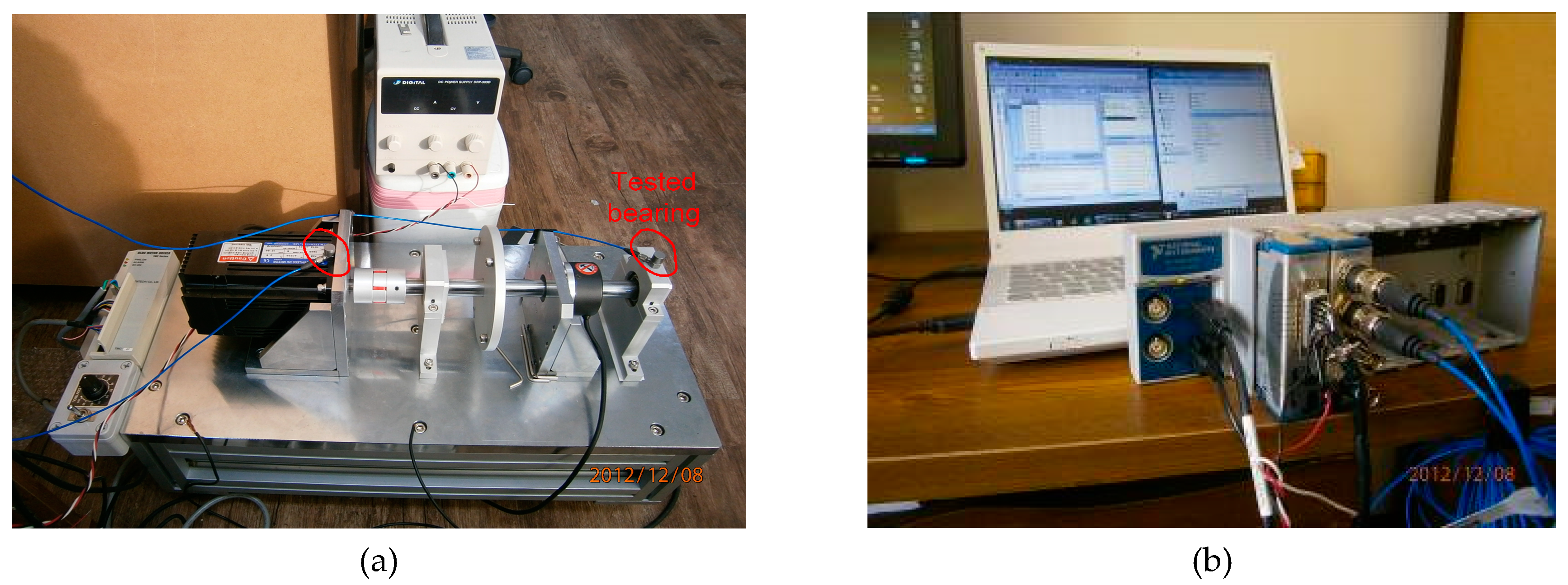
In order to evaluate the performances of the proposed ProbPlot via IR-AVPCA algorithm for bearing fault detection and diagnosis, an experimental setup with a 750W BLDC motor powered by a TMC-7 BLDC motor driver (TM Tech Co., Ltd., Gyeonggi-do, 27-11, South Korea) for vibration-based bearing fault detection and diagnosis was conducted, as shown in Figure 4.

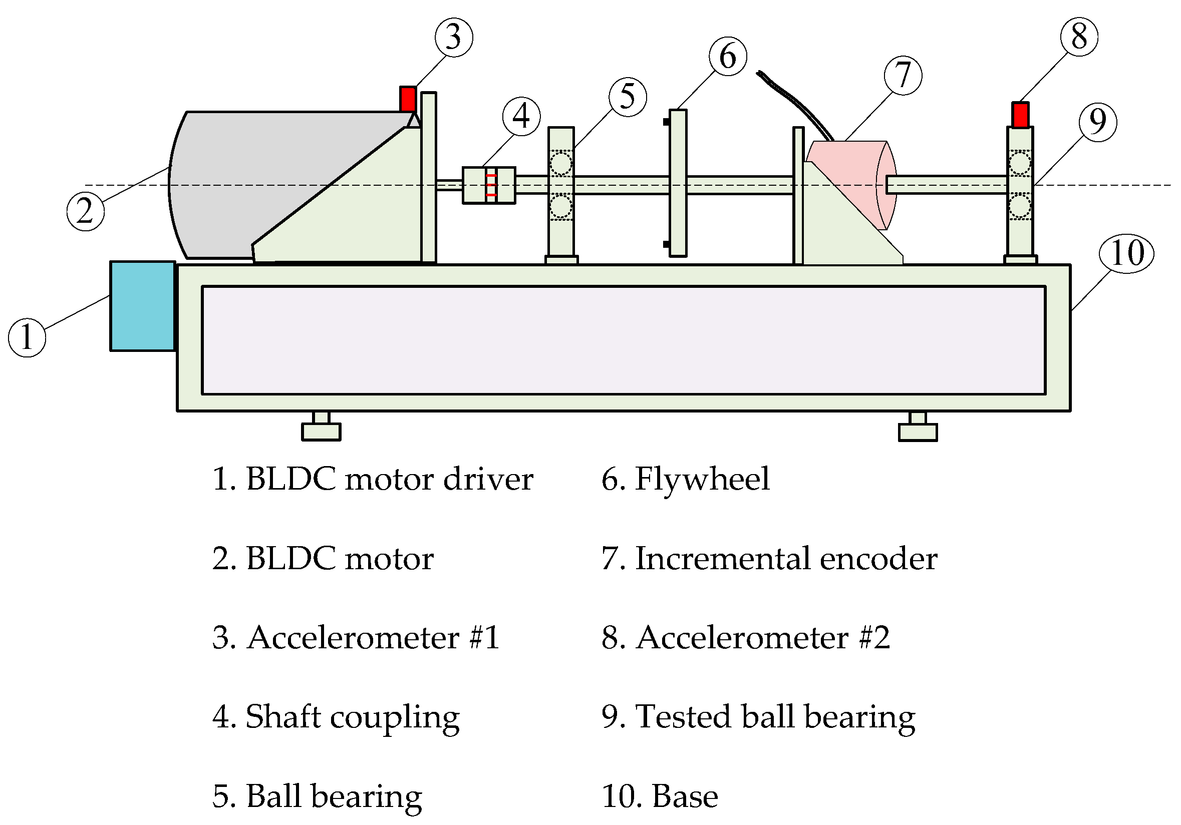
Two accelerometer sensors (model: 352C33 PCB) (PCB Piezotronics, Inc., International Distributors, Gyeonggi-do, South Korea.) were used to gather the vibration signals; the first was set up on the top of the BLDC motor to be a reference, and the second was installed above the tested bearing (NSK 6204 with eight balls type) (see Figure 5). The different bearing faults, i.e., ORF, IRF, and BBF, were artificially created by drilling axially a 1 mm hole through the outer-race, the inner-race, and the ball, respectively.

A constant load torque was added to the experimental test-bench by attaching a flywheel just before the tested bearing. NI cDAQ-9178 8-slot USB chassis was used to acquire the required vibration signals with the use of the NI9234 module. A 17.06 kHz sampling frequency was considered for sampling and Matlab R2012a was considered for processing.

Two different environments were considered: a constant speed environment and a variable speed environment.

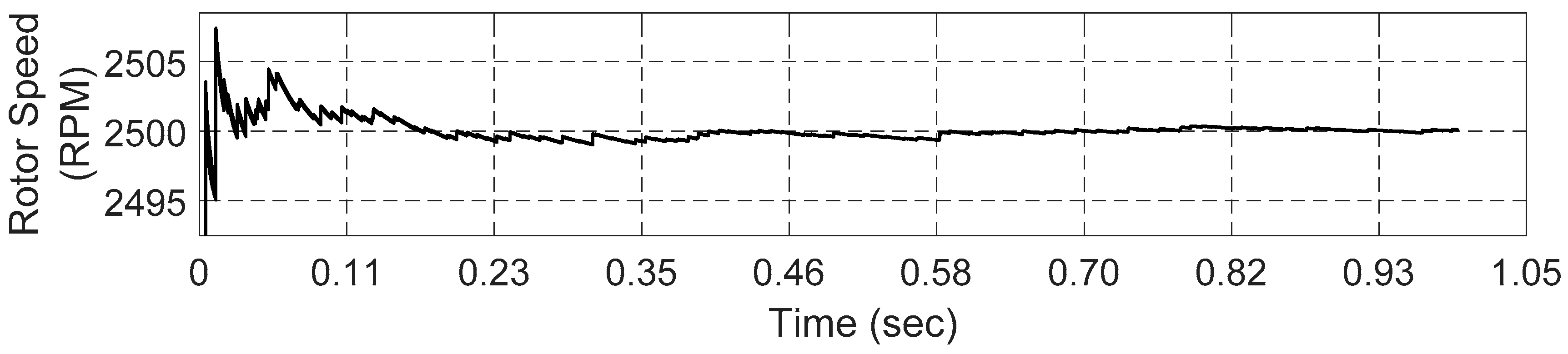
First, a constant motor speed of w_r = 2500 rpm was considered while the vibration-based bearing fault detection and diagnosis algorithm was running, see Figure 6.

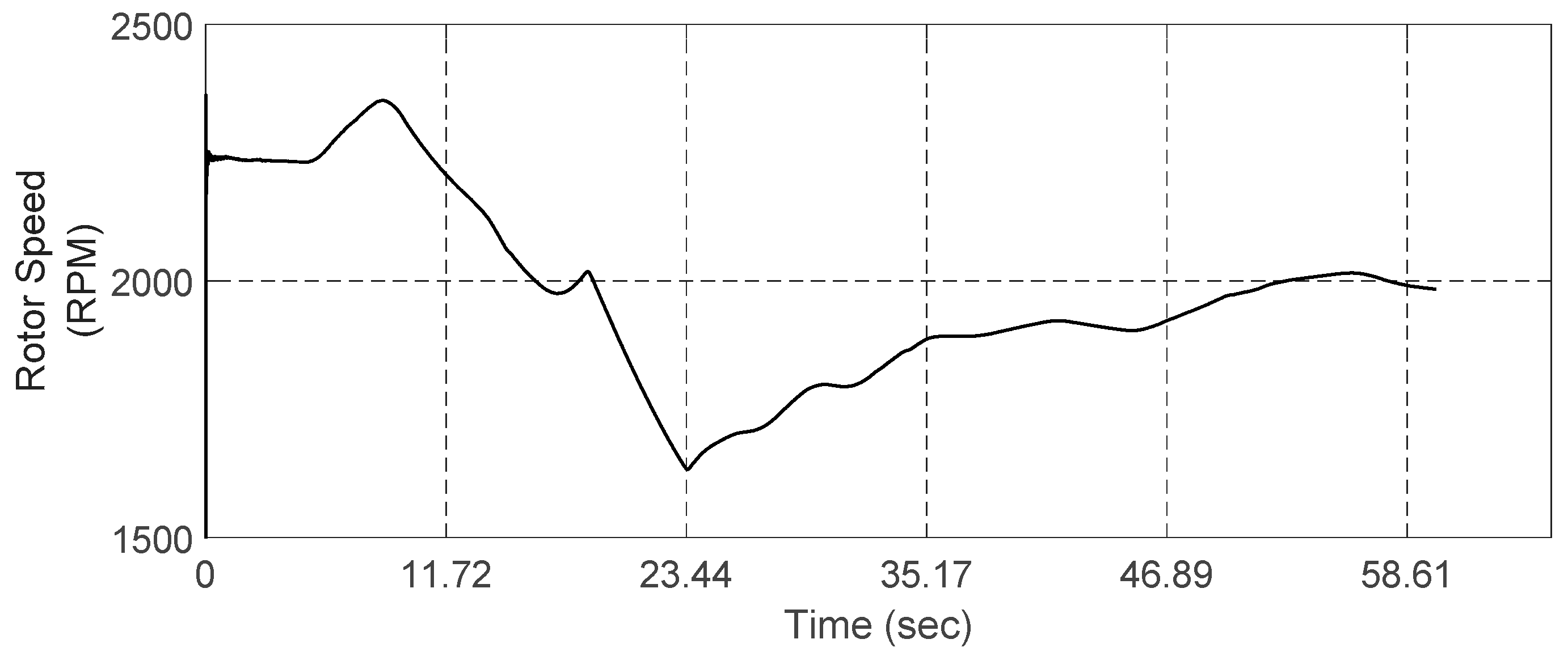
Second, a variable motor speed of w_r ϵ [1600, 2400] rpm was considered while the vibration-based bearing fault detection and diagnosis algorithm was running, see Figure 7.

The used dataset description is shown in

Table 1. Description of the used dataset.

Data Type	Label (m)	Number of Samples
		Constant Speed Environment	Variable Speed Environment
BFF	1	17,060	1,024,000
ORF	2	17,060	1,024,000
IRF	3	17,060	1,024,000
BBF	4	17,060	1,024,000

.

3.1. ProbPlot via IR-AVPCA to Online Fault Detection and Diagnosis Under Constant Speed

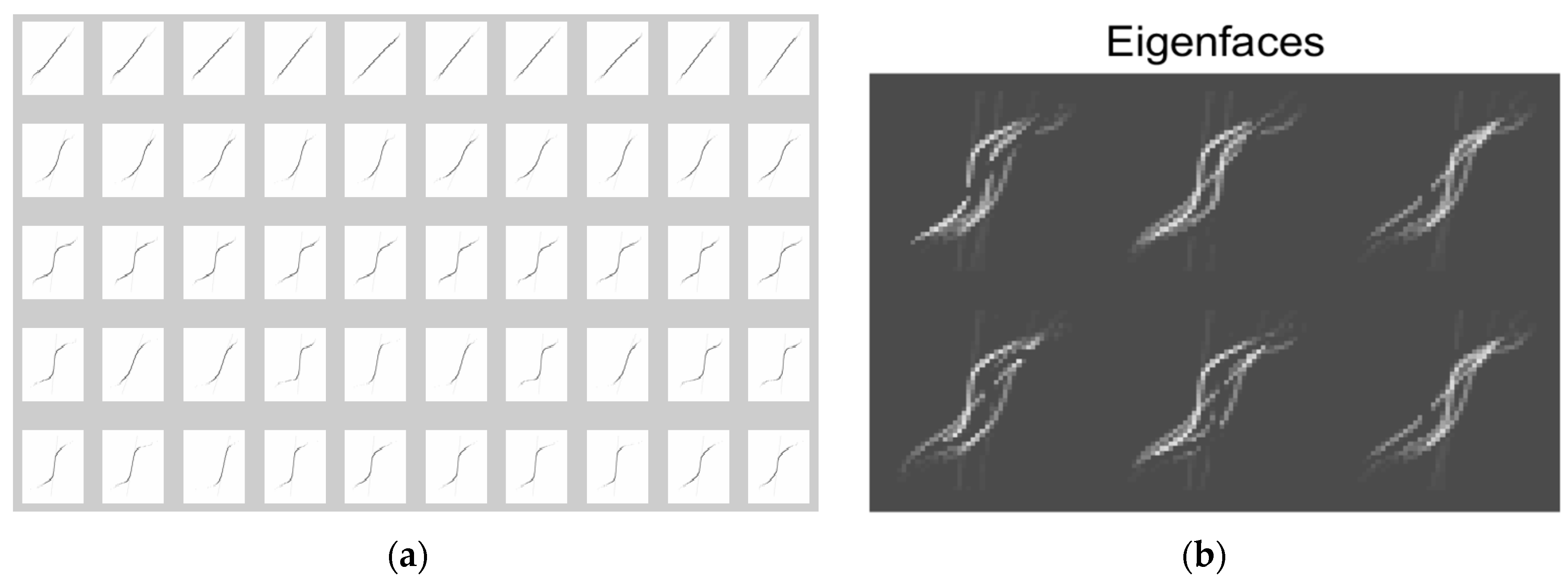
After getting all ProbPlot of the raw vibration data signal for each case, the m features (in which m = 1, 2, 3, 4) were generated in Matlab as an image of 100 dpi (dots per inch) and of 800 × 600 pixels. Then, each feature was projected to the AVPCA subspace to generate the training databases that contain the healthy base vector and the faulty base matrix. The training databases and the generated eigenfaces for each operating health condition can be seen in Figure 8a,b, respectively.

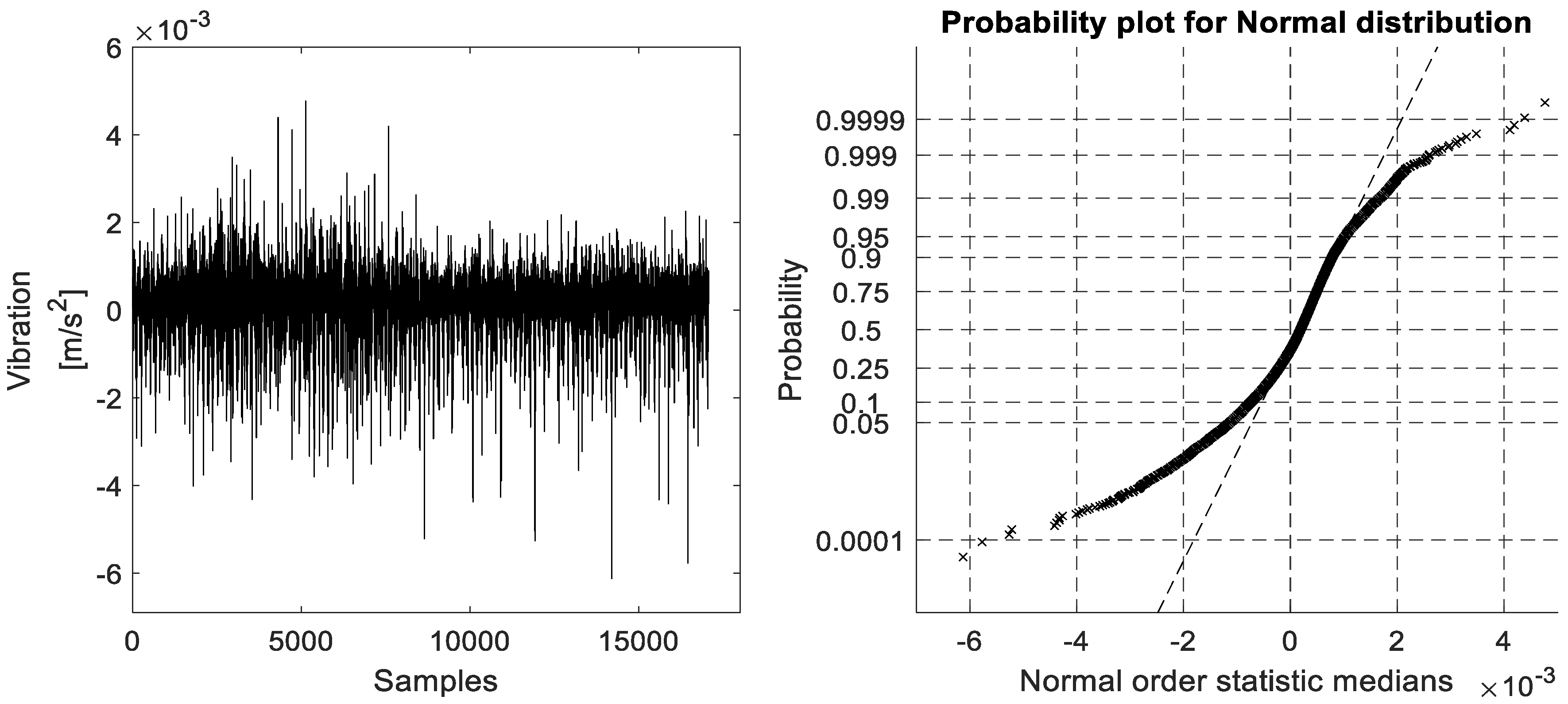
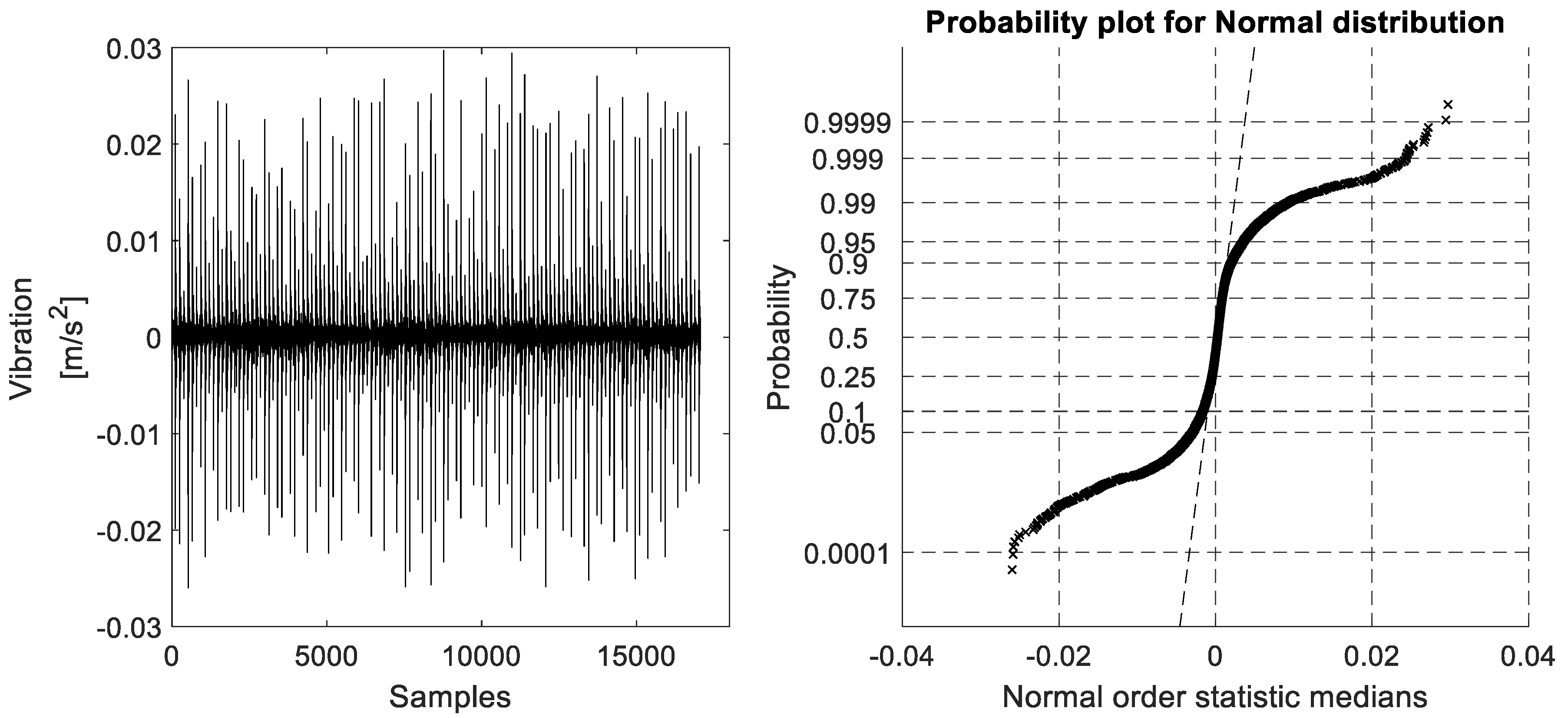
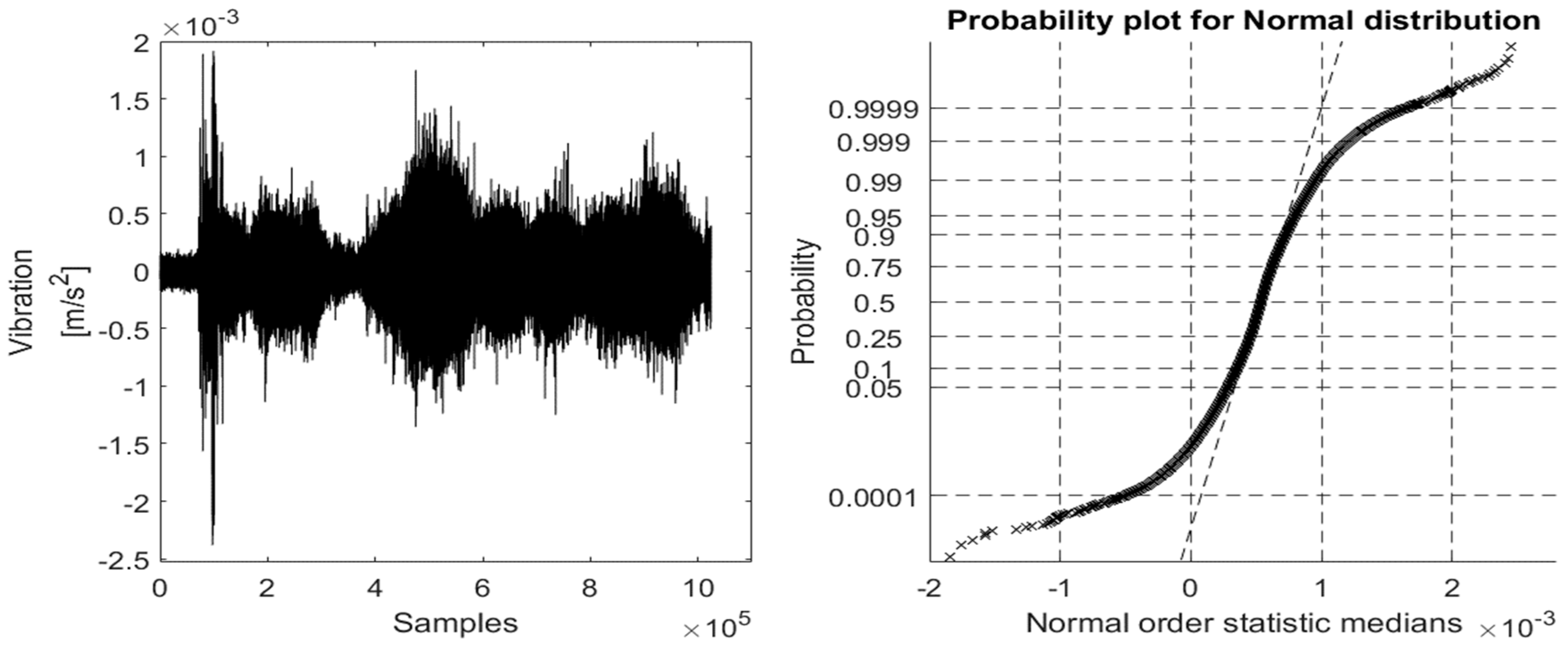
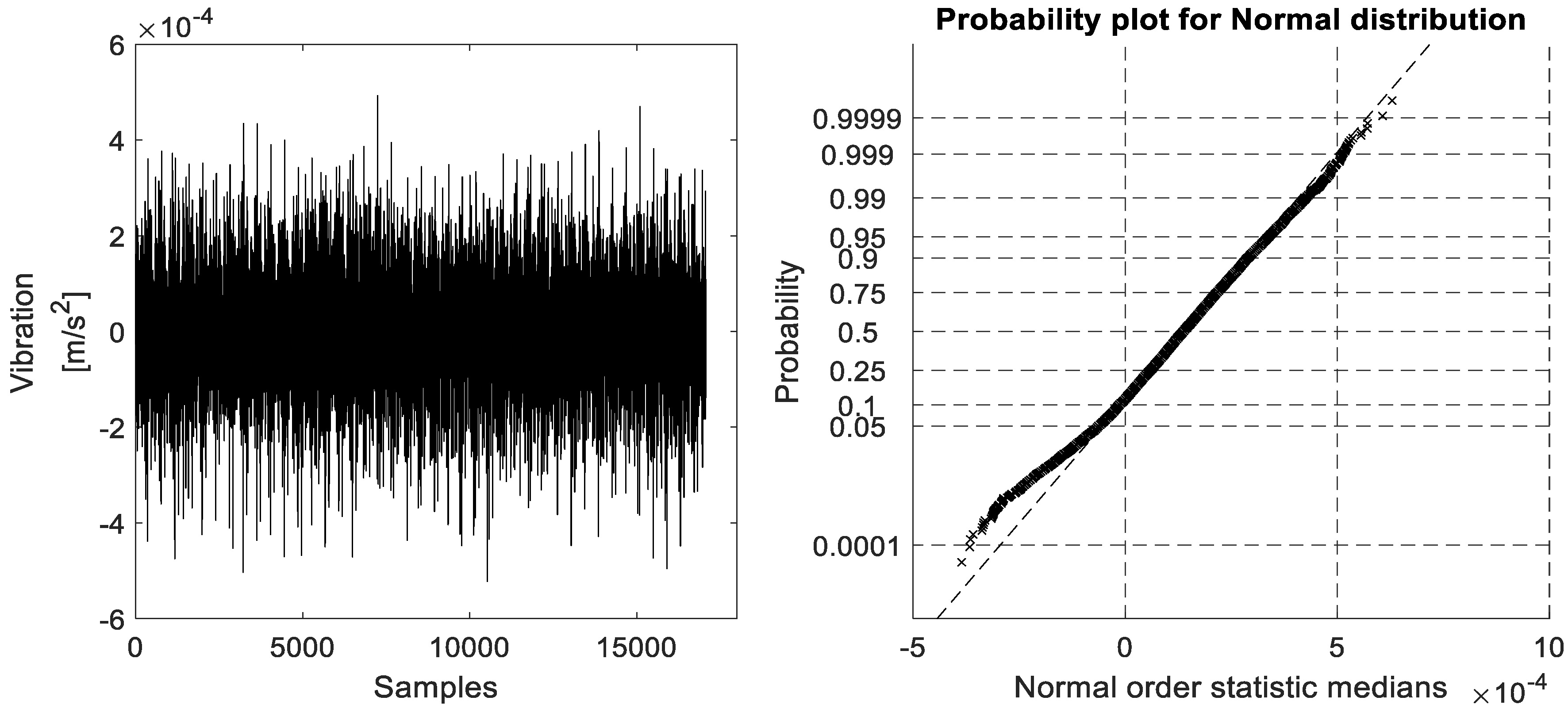
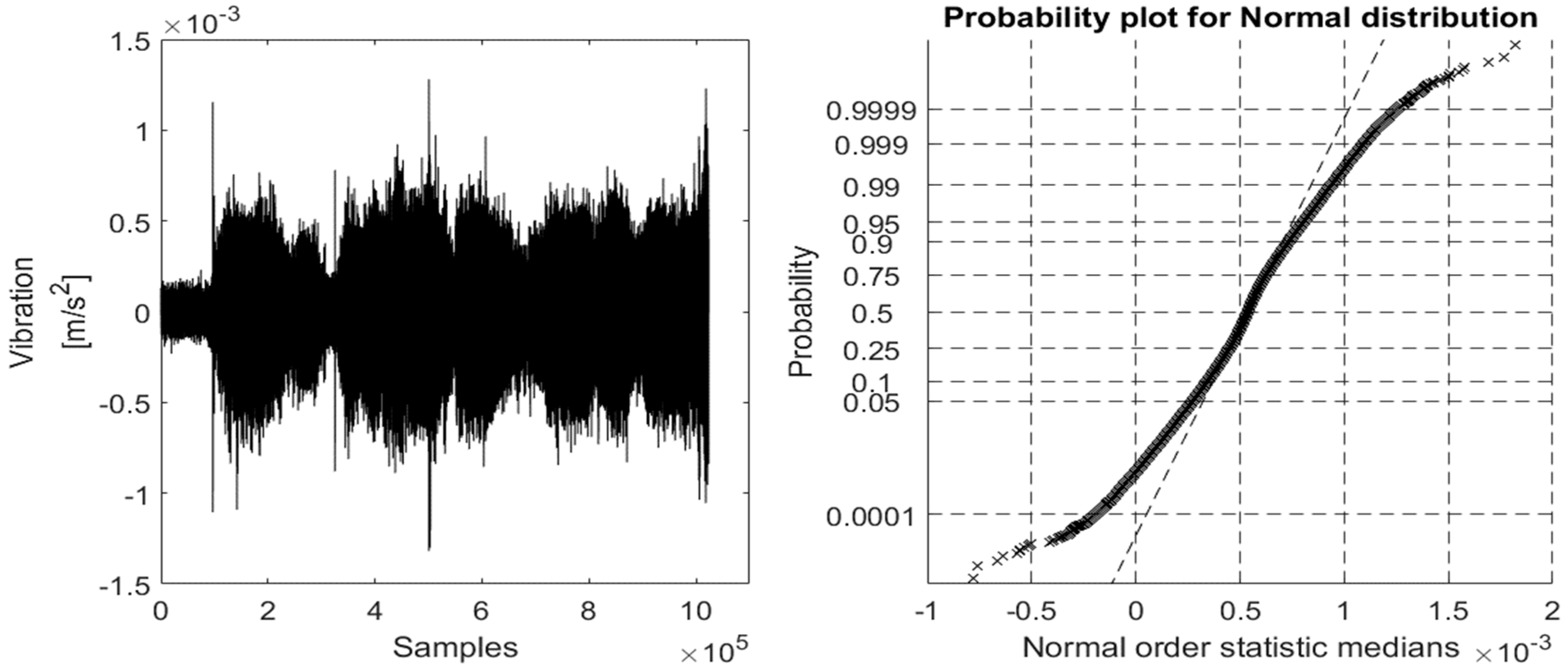
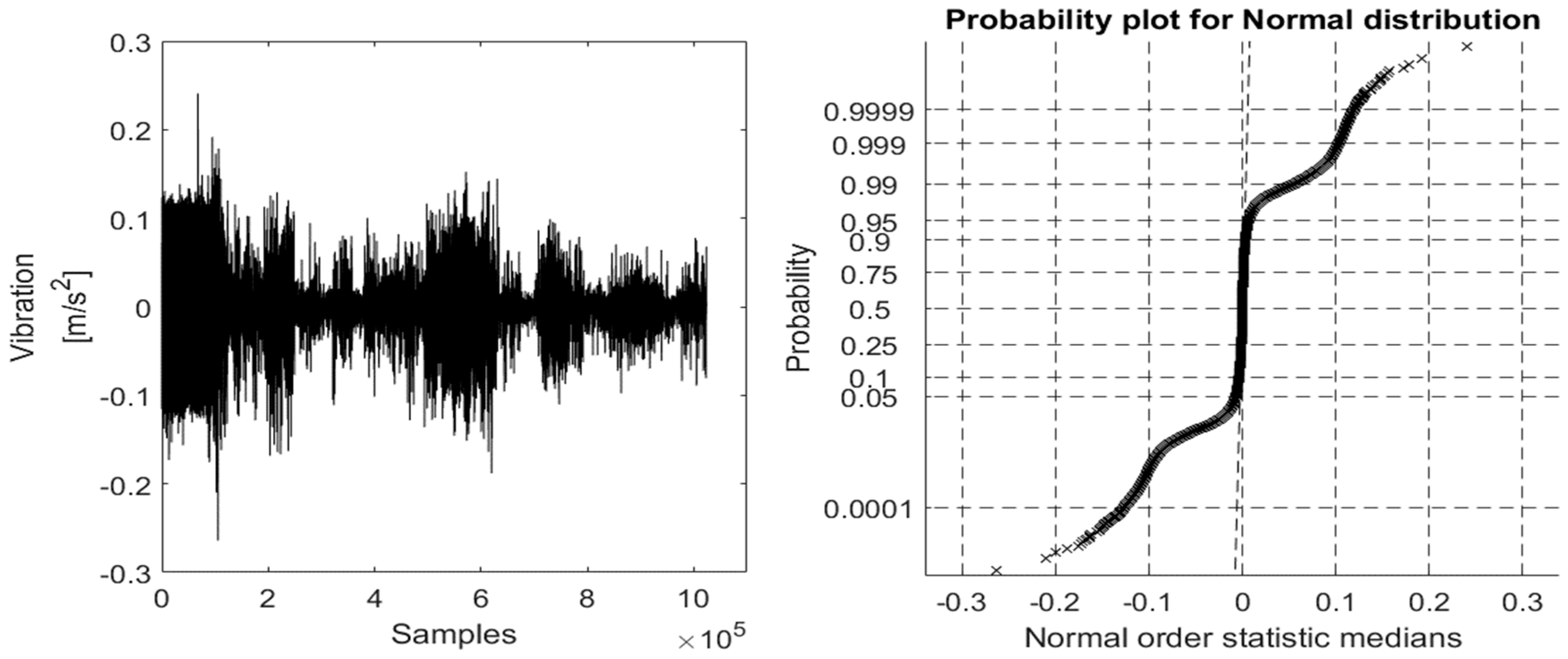
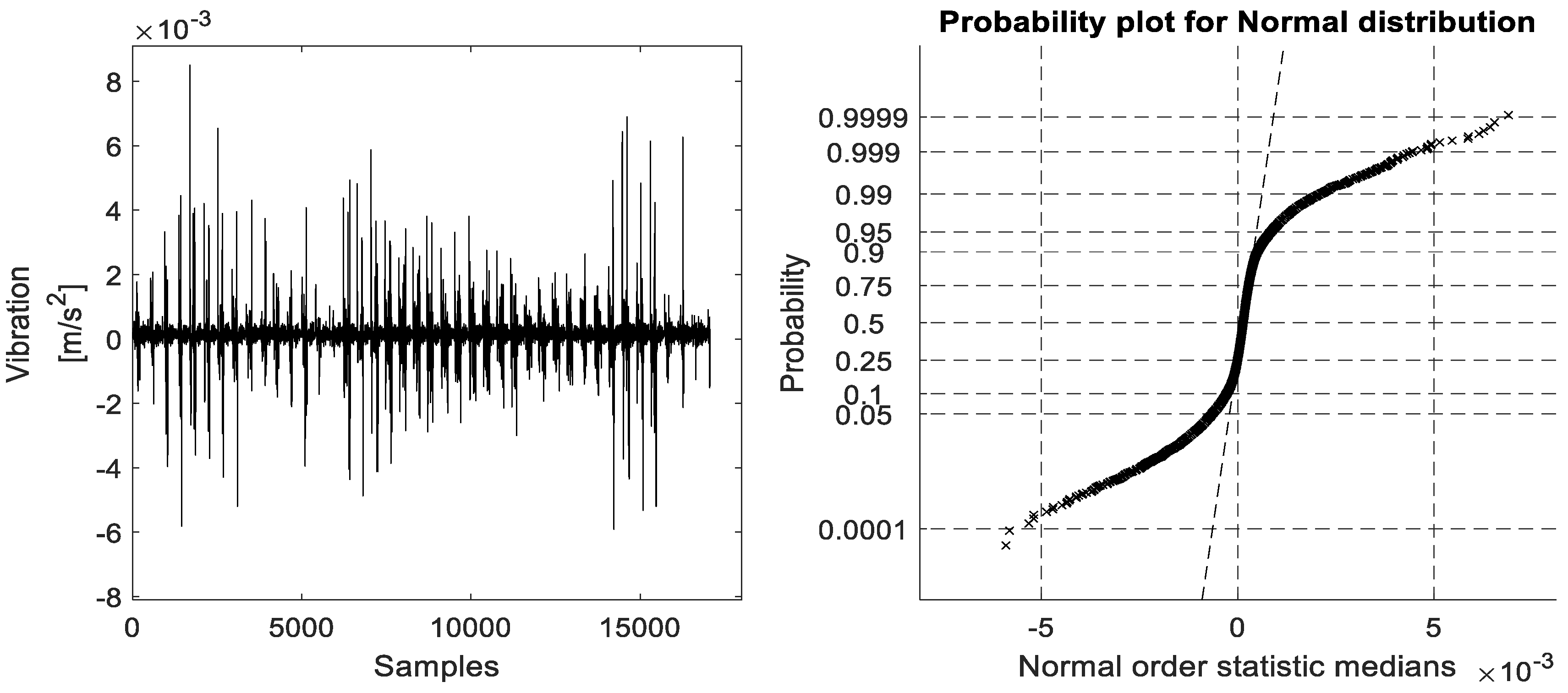
The raw vibration data signal acquired from accelerometer #1 (located on the top of the BLDC motor as shown in Figure 5) and its ProbPlot under constant speed environment are given in Figure 9, whereas the raw vibration data signals acquired from accelerometer #2 (located on the tested bearing housing as shown in Figure 5), its ProbPlot in bearing fault free (BFF) case and the different bearing fault cases (ORF, IRF, and BBF), and its ProbPlots under constant speed environment are shown in Figure 10, Figure 11, Figure 12 and Figure 13, respectively. It should be noted that in Figure 9, the ProbPlot of the vibration signal collected from accelerometer #1 shows a very straight line following the normal order statistic medians. This implies that the considered experimental bearing faults were very small, in which their impact could not affect the vibration signals collected from above the BLDC motor.

3.2. ProbPlot via IR-AVPCA to Online Fault Detection and Diagnosis Under Variable Speed

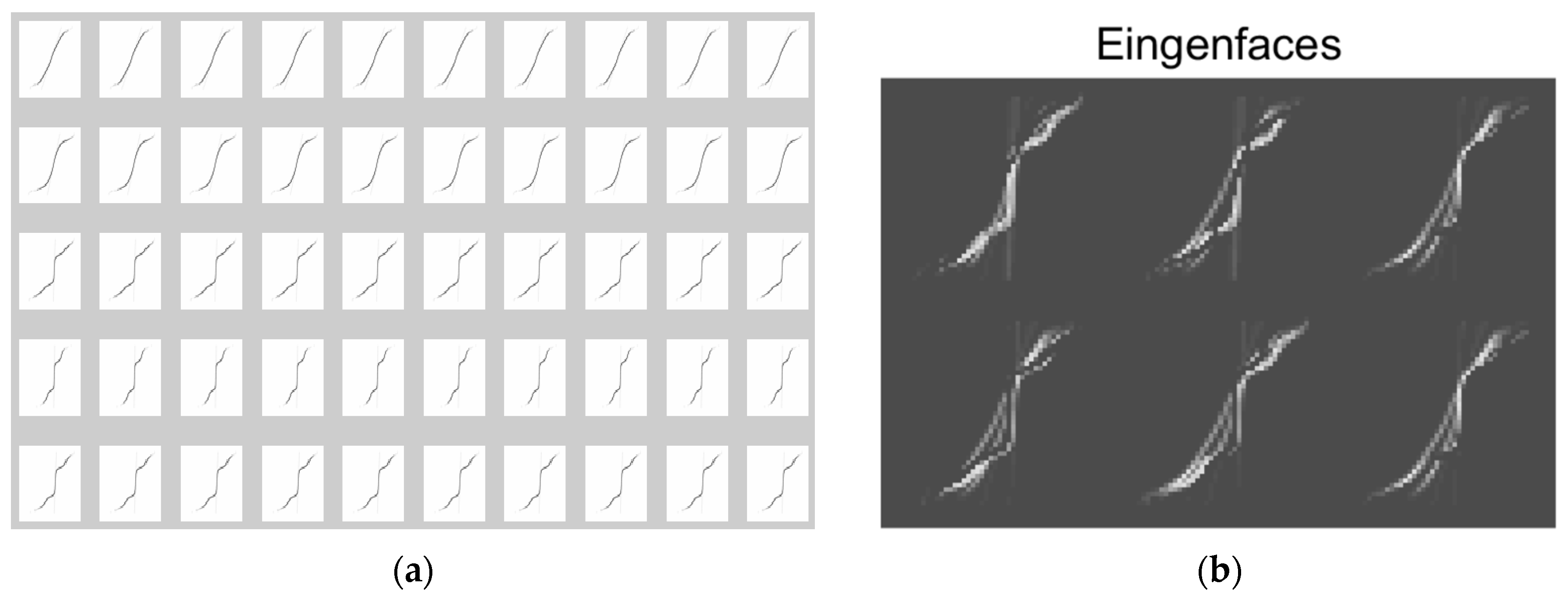
The m features were also generated in Matlab as an image of 100 dpi and of 800 × 600 pixels. Then, each feature was projected to the AVPCA subspace to generate the training databases that contain the healthy base vector and the faulty base matrix. The training databases and the generated eigenfaces for each four faulty cases under the variable speed condition can be seen in Figure 14a,b, respectively.

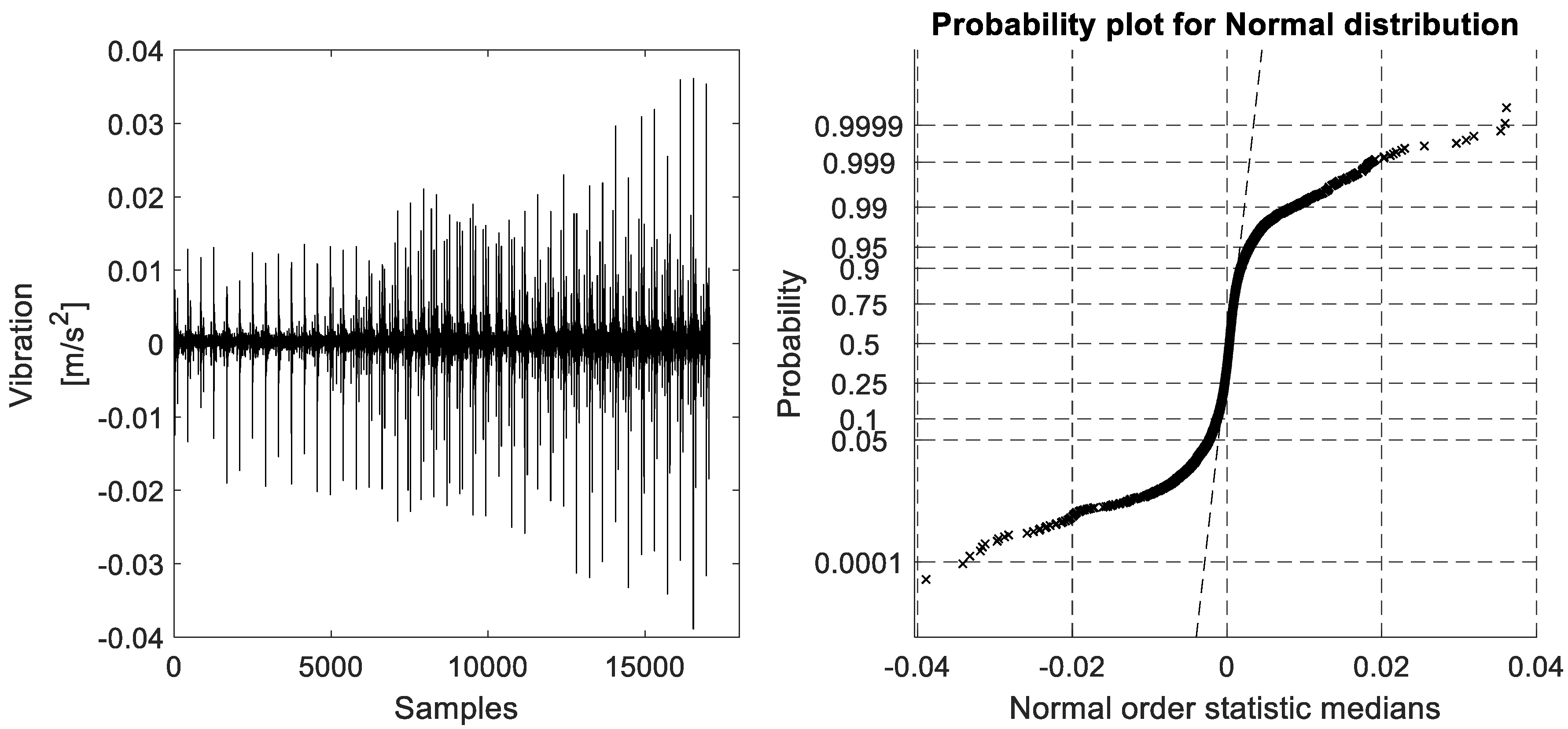
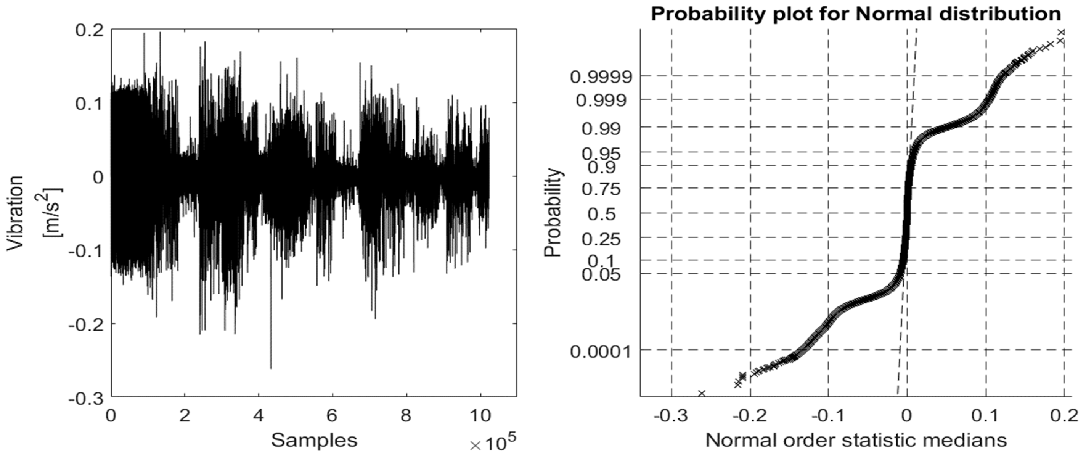
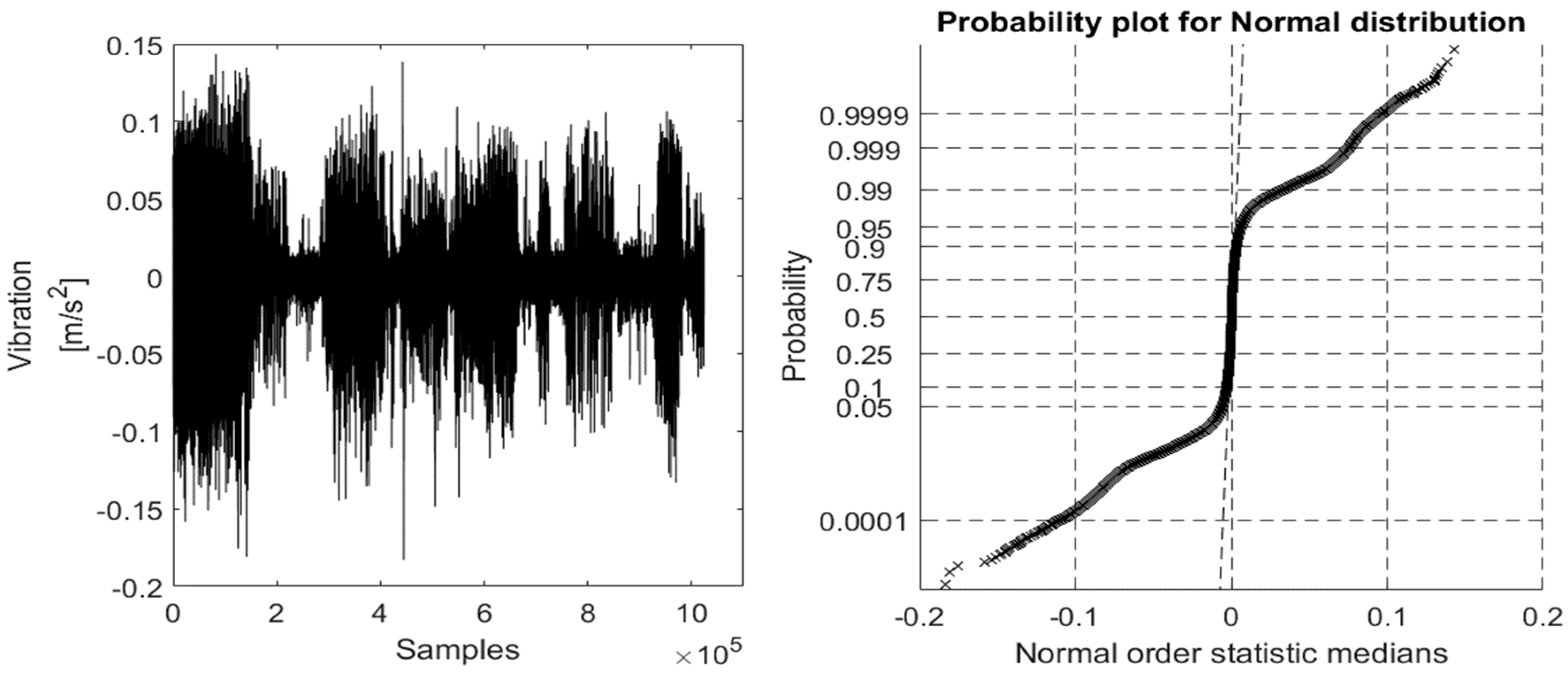
As for the constant speed environment, the vibration signal that was collected from the accelerometer #1 & #2, which was gathered on the four different operating health conditions (BFF, ORF, IRF, and BBF), and the reference one that was located on the top of the BLDC motor under the variable speed environment that was varying between 1600 rpm and 2400 rpm for 60 s under 17.06 kHz sampling rate with its ProbPlot for each, are shown in Figure 15, Figure 16, Figure 17, Figure 18 and Figure 19. Figure 15 again clarifies the conclusion drawn from Figure 9 and shows clearly that the considered experimental bearing faults are early bearing fault scenarios. However, the ProbPlot in Figure 15 shows more deviation in the normal order statistic medians than the one in Figure 9. These results come from the effect of the variable speed condition considered in the second environment.

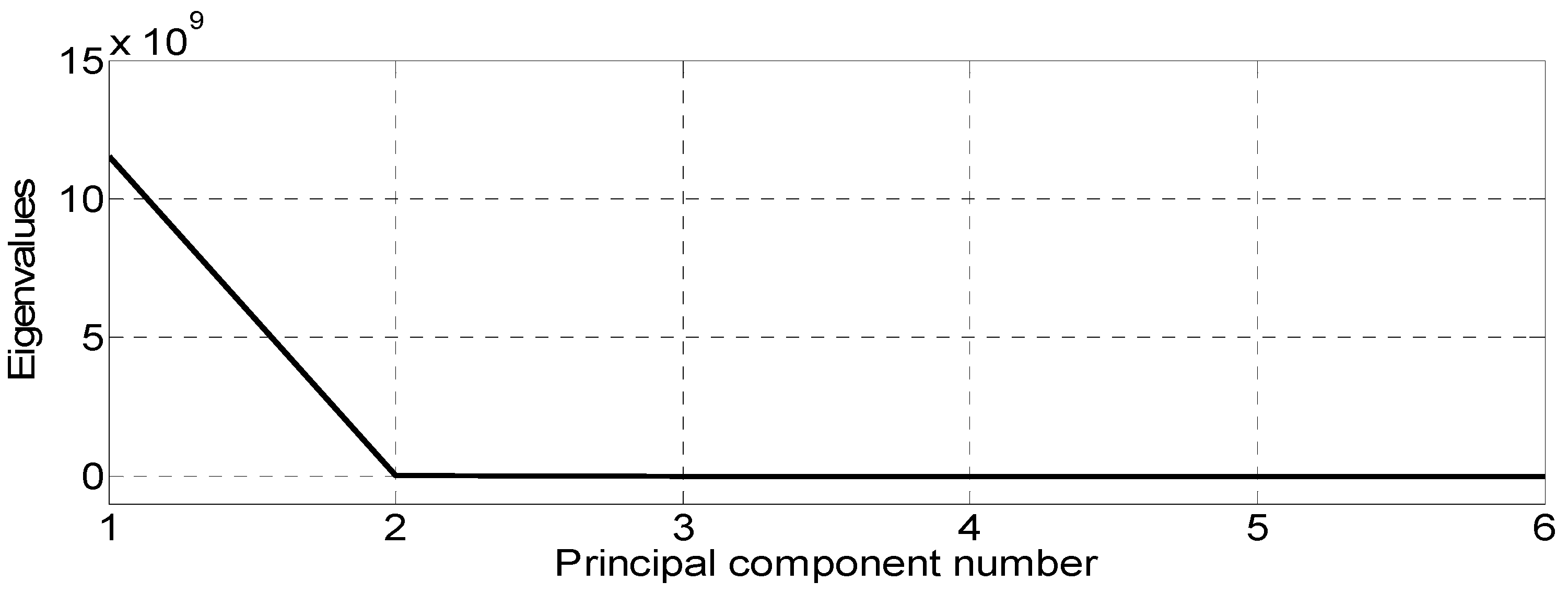
After projection to the AVPCA subspace, the dimension was reduced to one dimension, as can be seen in Figure 20, in which the SCREE [40] plot indicates that the number of retained principal components (PCs) can be chosen as one (p = 1). Using the cumulative percent of variance (CPV) criteria defined as, respectively,

$$CPV\left(p\right)=100·{\displaystyle \sum }_{i=1}^p\frac{{\lambda }_i}{{{\displaystyle \sum }}_{i=1}^n{\lambda }_i}$$

(10)

indicates that for p = 1, the CPV = 99.76%, which means that by only considering the one-space (the 1st eigenvector that corresponds to the largest eigenvalue), we could reach only 99.76% of precision. Thus, to reach at least a 99.95% precision, the number of retained PCs is fixed at six (p = 6), as shown in

Table 2. CPV precision of the eigenvalues.

PC Number	1	2	3	4	5	6
Eigenvalues	11.4 × 109	4.63 × 10−3	3.49 × 10−4	8.04 × 10−5	4.51 × 10−6	3.67 × 10−6
CPV (%)	99.76	99.83	99.87	99.91	99.94	99.96

.

A comparison between the features (images) that are obtained: (1) directly in the time domain from the original raw data of the vibration signals; (2) by capturing the Fast Fourier Transformation (FFT) of the vibration signals as in [23]; and (3) by generating the ProbPlot of the vibration signals as proposed in this paper, is considered to demonstrate the performance and effectiveness of the proposed ProbPlot via IR-AVPCA method at online bearing fault detection and diagnosis. Furthermore, both classical PCA and AVPCA are used and compared in terms of bearing faults classification success rate. It should be noted that for the second working conditions (i.e., nonstationary conditions under variable speed environment), the proposed algorithm is compared only to the first case (i.e., when directly generating the features (images) from the raw vibration data), since the FFT is not convenient under those operating conditions in which the needed bearing fault information that changes over time will be lost.

The summary of the online bearing fault detection and diagnosis (BFDD) for the different features (images) generation methods and its success-rate with both classical PCA and AVPCA under both constant and variable speed environments is given in

Table 3. Summary of proposed ProbPlot via IR-AVPCA-based BFDD efficiency for the different features (images) generation methods using PCA and AVPCA algorithms under both constant and variable speed environments.

			Constant Speed				Variable Speed
		Task	Fault Detection	Fault Diagnosis			Fault Detection	Fault Diagnosis
Method
Success rate (%)	Classical PCA	Features (images) are obtained from the raw vibration data signal	BFF	ORF	IRF	BBF	BFF	ORF	IRF	BBF
			68	68	62.67	60	49.33	40	38.67	34.67
				Average: 63.56				Average: 37.78
		Features are captured after the FFT of the vibration signal	BFF	ORF	IRF	BBF	BFF	ORF	IRF	BBF
			86.67	82.67	78.67	80	-	-	-	-
				Average: 80.44				Average: -
		Features are generated using the proposed ProbPlot technique	BFF	ORF	IRF	BBF	BFF	ORF	IRF	BBF
			89.33	85.33	85.33	82.67	81.33	77.33	78.67	72
				Average: 84.43				Average: 76
	AVPCA	Features (images) are obtained from the raw vibration data signal	BFF	ORF	IRF	BBF	BFF	ORF	IRF	BBF
			78.67	78.67	76	76	68	72	62.67	65.33
				Average: 76.89				Average: 66.67
		Features are captured after the FFT of the vibration signal	BFF	ORF	IRF	BBF	BFF	ORF	IRF	BBF
			97.33	98.67	96	94.67	-	-	-	-
				Average: 96.44				Average: -
		Features are generated using the proposed ProbPlot technique	BFF	ORF	IRF	BBF	BFF	ORF	IRF	BBF
			100	100	97.33	97.33	98.67	96	98.67	92
				Average: 98.22				Average: 95.56

.

3.3. Discussion

3.3.1. Under Constant Speed Environment

Table 3 shows that the AVPCA could detect the different bearing faults with a 78.67%, 97.33%, and 100% success rate (i.e., fault detection rate) for the features (images) generating method using the raw vibration signal, the generating method after capturing the FFT of the vibration signal, and the generating method using the proposed ProbPlot technique, respectively. However, the classical PCA could detect the different bearing faults with only a 68%, 86.67%, and 89.33% success rate, respectively. A similar result was obtained for the fault diagnosis; the average success rates with the AVPCA were 76.89%, 96.44%, and 98.22%, and with the classical PCA they were 63.56%, 80.44%, and 84.43%, respectively. Thus, using the AVPCA improves both fault detection and diagnosis capability.

Furthermore, these results show clearly the advantage of generating the features (images) using the proposed ProbPlot technique (100% success rate for fault detection and 98.22% success rate for fault diagnosis) compared to the FFT of the vibration signal (97.33% success rate for fault detection and 96.44% success rate for fault diagnosis) or directly considering the image of the raw vibration signal (78.67% success rate for fault detection and 76.89% success rate for fault diagnosis).

3.3.2. Under Variable Speed Environment

Under variable speed environment, which is a more challenging though more realistic situation, the AVPCA was capable of detecting the bearing fault with 68% and 98.67% success rate for the different features generating methods (image of raw vibration data, signal, and image of the ProbPlot of the vibration signal), respectively, and could diagnose those detected fault with a 66.67% and 95.56% average success rate. In contrast, the classical PCA did detect the bearing fault with only a 49.33% and 81.33% success rate, respectively, for the two features generating methods and did diagnose the detected faults with only 37.78% and 76% average success rate, respectively.

Furthermore, these results show clearly the advantage of generating the features (images) using the proposed ProbPlot technique (98.67% success rate for fault detection and 95.56% average success rate for fault diagnosis) compared to directly considering the image of the raw vibration signal (68% success rate for fault detection and 66.67% average success rate for fault diagnosis) under variable speed environment.

In addition, the proposed ProbPlot technique is more suitable for online bearing fault detection and diagnosis and for being adapted to real industrial applications, since it does not require any computation or space compared to the use of the FFT of the vibration signals, and since it can detect and diagnose the different bearing faults under nonstationary conditions, unlike the FFT.

4. Conclusions

In this paper, a novel image recognition technique for bearing fault detection and diagnosis, the ProbPlot via IR-AVPCA, was proposed. The generated features (images) of the vibration signals were simply obtained by plotting the probability plot (ProbPlot) of the vibration signal. Using the AVPCA, the eigenfaces were extracted, and the bases were generated. Then, a notion of the total sum square error (SSE) distances and its minimum was used to detect and diagnose the three different bearing faults (outer-race fault (ORF), inner-race fault (IRF), and ball fault (BBF)).

The proposed algorithm was examined under constant and variable speed environments. A set of experiments with artificially introduced faults was considered, and its results showed that the proposed ProbPlot via IR-AVPCA technique was the best method in terms of detecting and diagnosing the bearing faults for both constant speed and variable speed environments. Further, since it does not require any computation or space compared to the use of the FFT of the vibration signals, the proposed technique will be more suitable for the online bearing fault detection and diagnosis and for being adapted to real industrial applications, especially since it can deal with the BFDD under nonstationary conditions, unlike the FFT, which cannot.

For future work, the proposed ProbPlot via IR-AVPCA technique will be further investigated for gearbox fault detection and diagnosis and then for bearing fault prognosis.