Acoustic Emission Monitoring of Industrial Facilities under Static and Cyclic Loading

Featured Application

Structure health monitoring for refinery equipment, bridges, rotating machines, cranes and draglines.

Abstract

Acoustic emission (AE) testing is traditionally carried out on non-operating objects. Such requirement is associated both with the Kaiser effect, leading to the necessity for exceeding the test load above the working one and with a high level of noise during object operation. However, AE testing could be performed under operating conditions, if the AE data acquisition period is increased and a specialized method is developed, which should take account of the effect of various noise, features of the object loading under operating conditions, the effect of damaging factors and possible destruction mechanisms. This paper investigates the possibility to carry out structural health monitoring (SHM) of hydrotreaters, highway bridges, high-temperature pipelines, gas adsorbers, roller bearings of rotary kilns and draglines on the basis of AE method. Architecture of SHM-system and specific data analysis procedures are proposed.

1. Introduction

Nowadays the status of complex (especially dangerous) industrial structures is widely assessed by structural health monitoring (SHM), that is the continuous evaluation of their structural heath [1]. The main reasons to apply SHM are:

• access to the structure during operation is difficult or impossible;
• periodic nondestructive testing (NDT) is not possible or is time-consuming;
• temporary stoppage of equipment for its testing induces large financial losses;
• rapid development of operational defects and, as a result, low damage tolerance of the structure;
• the consequences of structural failure, which can lead to large material losses and a danger for maintenance personnel;
• the presence of known defects when it is necessary to extend the lifetime of the equipment.

SHM of equipment allows the early detection of most of the failures and alerts maintenance personnel about developing malfunction that already exists but is not yet dangerous and does not disrupt the operability of the equipment. Among various NDT methods, the acoustic emission (AE) method is the most effective one in the monitoring mode. This method due to the possibility of remote testing and high sensitivity in the crack detection allows real-time monitoring of the structures with a length of up to several hundred meters. It is important to emphasize that the detectability of a defect is not affected by its orientation. AE method makes it possible to detect the following types of defects: cracks, microcracks, various types of corrosion damage and leaks [2]. Despite all the advantages of AE method, other types of testing should be used to provide a more accurate and objective assessment of the structural health [3,4,5,6,7]. This is caused by several reasons: firstly, in the case of usual AE testing, a temporarily decommissioned structure must be additionally loaded to stimulate the growth of the defects, while in the monitoring mode this need disappears, since testing is performed continually and AE sources emit under the influence of variations in operational loads, the value of which is not precisely known. Therefore, it must be ensured that the almost unlimited time of the AE testing can compensate the reduced magnitude of the load changes. Secondly, AE testing in the monitoring mode is complicated by increased process acoustic noise of the equipment. Experience in the use of monitoring systems shows that under such conditions defects are reliably detected only at the final stages of destruction, when the number of AE signals and their amplitudes increase by more than an order of magnitude. All this leads to the need of complex monitoring, that is the use of AE method with other NDT methods, as well as with the tracking of operational parameters.

Also, the design and implementation of structural health monitoring system (SHM-system) should always take into account the specificity of the monitored structures. It is necessary first to study the design features of the structure and the results of previous investigations, analyze the types of loads and factors that generate defects [8]. For the determination of the zones in the structure, in which the occurrence of cracks is most likely, the stress-strain state of the structure can be numerically simulated. Then a complete investigation of the structure is carried out, usually with trial AE testing. As a result, the acoustic parameters of the structure are determined, with the types of possible defects, their nature of developing, reasons of the formation, their most probable positions and their influence on the lifetime of the structure are revealed. Sufficiency of load changes for the stimulation of AE sources is estimated. After that, the selection of methods and instruments of NDT and the positions of the sensors are determined. In addition, in the course of preliminary work, noise filtering and data analysis procedures are developed for each specific structure (due to the large volume of primary data).

2. Methods

«INTERUNIS-IT» Limited Liability Company has developed SHM-systems for various structures and plants on the basis of A-Line AE system. SHM-system hardware is implemented as a distributed system for data collection and processing with digital data transfer. All components of SHM-system are built from the unified measuring devices and have a common control core. The proposed concept of SHM-system design implies the unification of different components into a single system:

• Monitoring by multiple NDT methods.
• Monitoring of the structure’s stress-strain state.
• Tracking of the working parameters of the industrial process [9]

SHM-system is a system designed to assess the diagnostics of hazardous matters in real time without stopping, dismantling and shut down. SHM-system provides information about the status of the monitoring facility in the required quantity and quality for testing. The structure of SHM-system includes the following functional elements: equipment for primary data collection, multifunctional data acquisition and transmission modules, concentrators, galvanic isolation switching cabinet and central computer station (Figure 1).

The equipment for primary data collection may include one or several types of acoustic emission sensors, strain gauges, corrosion rate meters; pH meters, vibration sensors, displacement meters and inclinometers, crack opening sensors; level gauges, thermocouples, pressure sensors, gas analyzers, video recorders and weather station. The specific composition varies depending on the structure and the goal of the monitoring.

Multifunctional data acquisition and transmission module is the main element of this architecture and is a separate device in an explosion-proof enclosure with installed cable entries. Each module contains several measuring units that collect data from external sensors of various types, and, if necessary, supply power to them. In particular, analogue filtering, digitization and digital filtering of signals, as well as calculation of AE parameters (such as arrival time, amplitude, duration, etc.) and the registration of waveforms are performed in a measuring unit intended for operation with an AE sensor. The total number of sensors connected to the module can be up to 6. In addition, module includes a digital processing unit, communication unit and power unit. Multifunctional data acquisition and transmission modules are connected in series with each other by a cable that provides power and relay the data through the cascaded line. The modules are placed, as a rule, near the sensors, which together with digital data transmission, achieve high interference immunity.

The concentrator is a separate device in an explosion-proof enclosure that receives information from several (up to 4) cascaded lines of modules and sends it further via the Ethernet interface.

The switching cabinet of the galvanic isolation carries out a galvanic isolation between the primary supply voltage of 220 V/50 Hz and the secondary direct current (DC) voltage of 48 V, as well as the galvanic isolation between the measuring units.

The central computer station, which is designed for receiving, transmitting, storing and analyzing data and for measuring channels control. The central computer station includes computing devices for data processing and storing, as well as a display and input devices, or a device for communicating with a remote-control terminal.

The SHM-system can also include an automated workstation—a remote terminal used for remote access to a central computer station, monitoring data processing and performing backups of information.

3. Results and Discussion

3.1. Hydrotreater of Oil Refinery Plant

3.1.1. SHM-System Location

Overheating caused by a run-away of the process induced the formation of defects at the hydrotreater at the oil refinery plant. During periodic AE testing, significant AE sources were detected and it was assumed that it is the destruction of the cladding layer. In December 2006, SHM-system was put into operation, the task of which was to ensure the safe operation of the hydrotreater with an extended lifespan until it is possible to replace it.

Structurally, the hydrotreater is a thick-walled vertical steel vessel. The inner surface of the hydrotreater is protected from the influence of an aggressive medium by a cladding layer. The high operating temperatures of the hydrotreater (from 320 °C to 425 °C), the aggressive environment and high operating pressure are factors that can lead to the generation and catastrophically rapid flaw growth, especially when the cladding layer is destroyed, which can induce hydrogen embrittlement and a decrease in the strength of the material.

The main diagnostic method of SHM-system was the method of AE testing. The AE handling part was represented by 18 AE sensors GT200UB (130–200 kHz), grouped into 6 belts, 4 on the hydrotreater shell and 1 belt on each lid. Sensors were mounted on waveguides to ensure the temperature allowed for the sensor is not exceeded. Temperature, vibration and pressure sensors were also installed. A threshold data acquisition algorithm was used. The threshold value was about 40 dB. The analog-to-digital converter (ADC) sampling rate was equal to 2 MHz.

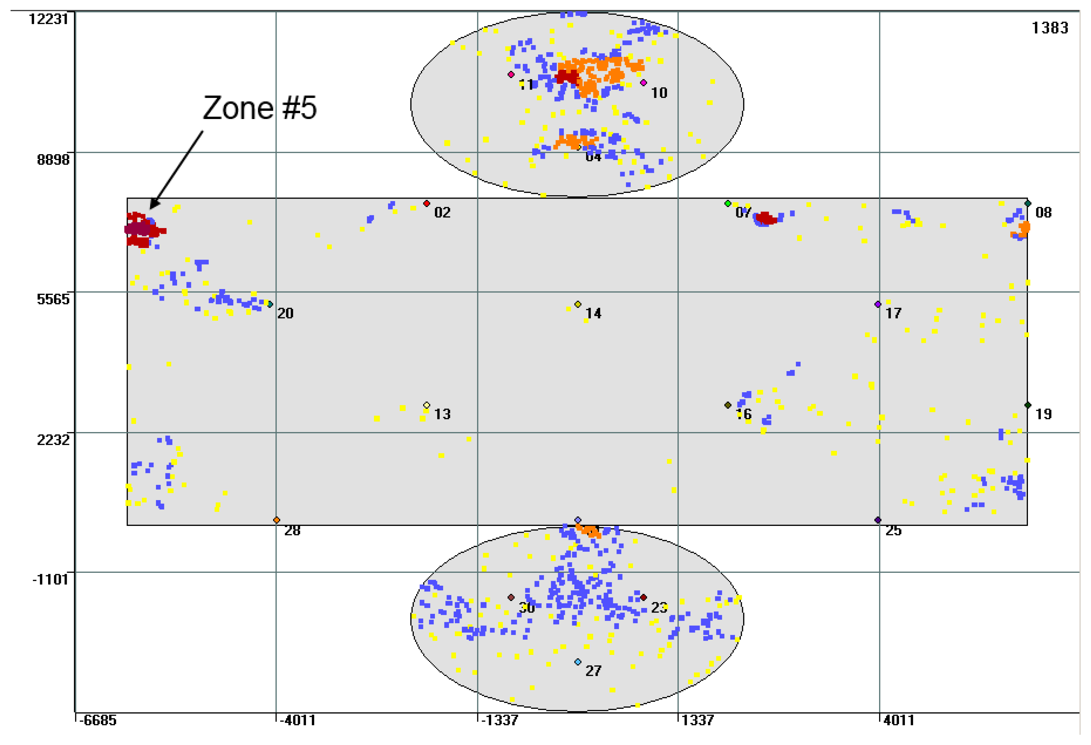
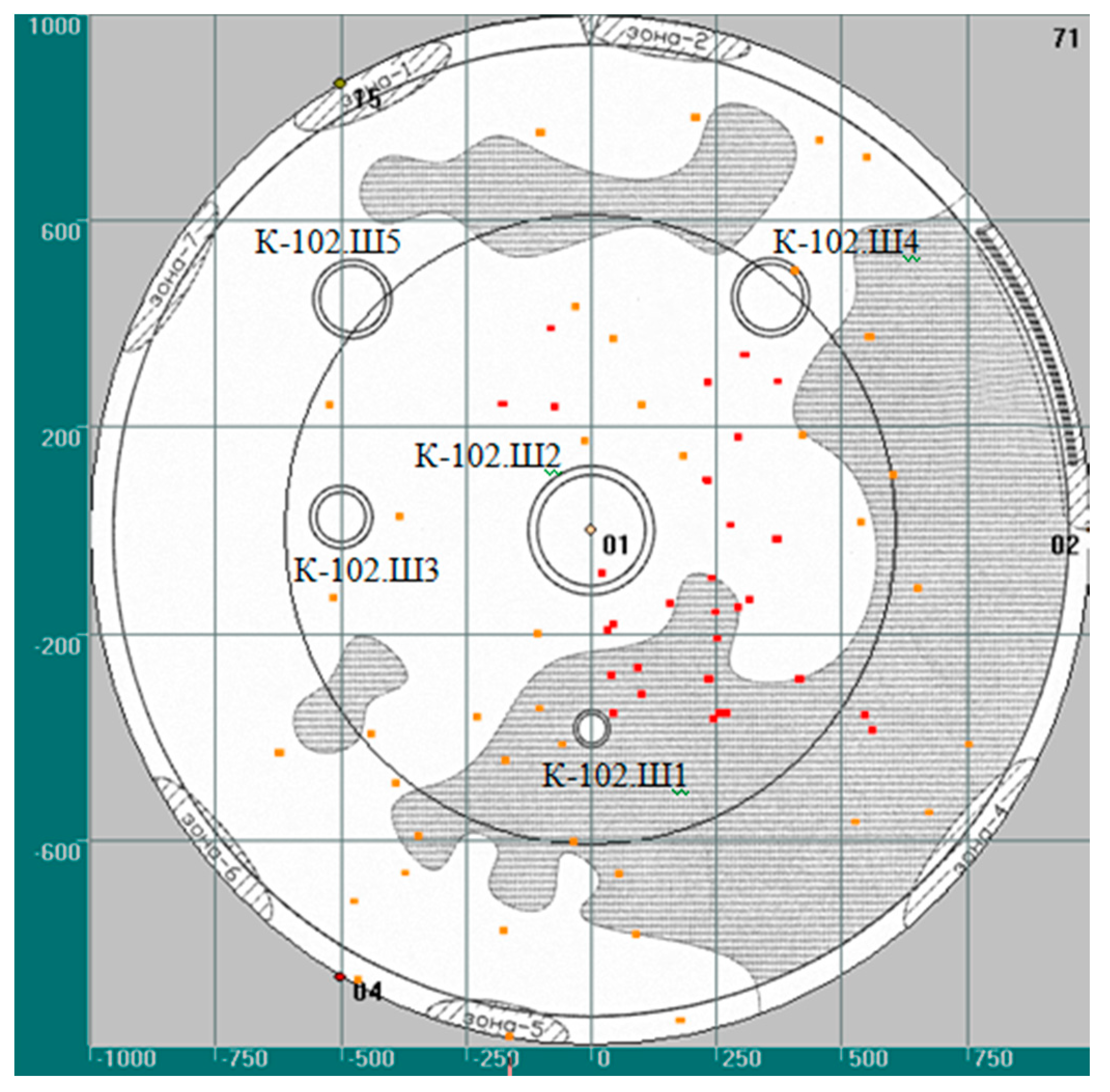
By May 2007, the state of the hydrotreater had deteriorated. It was found to have 9 active zones, corresponding to AE sources with varying degrees of danger (Figure 2). The activity of some zones increased significantly, which indicated a progressive flaw growth and the possibility of the hydrotreater destruction. The source found in zone #5 and characterized by 370 events, was considered to be critically active.

In order to resolve the issue of the time of decommissioning, it was decided to conduct additional analysis of monitored AE data.

3.1.2. Cluster Analysis of AE Data

After preliminary filtering, a cluster analysis of the AE data was carried out. AE signals were clustered for each measuring channel separately. As a measure of the similarity for each pair of signals, the correlation coefficient of their waveforms was used (threshold value was set to 0.7), or a measure based on the similarity between their AE parameters. As a result, "clusters of signals" were formed [10].

In total, about 500,000 AE signals were analyzed, including 65,000 waveforms. For AE signals registered by the channels testing zone #5, 23 clusters were formed. While conducting cluster analysis, 14 clusters was attributed to process-induced AE events, 4 clusters corresponded to the correlated noise and 5 clusters were characterized as the sources of AE with high probability.

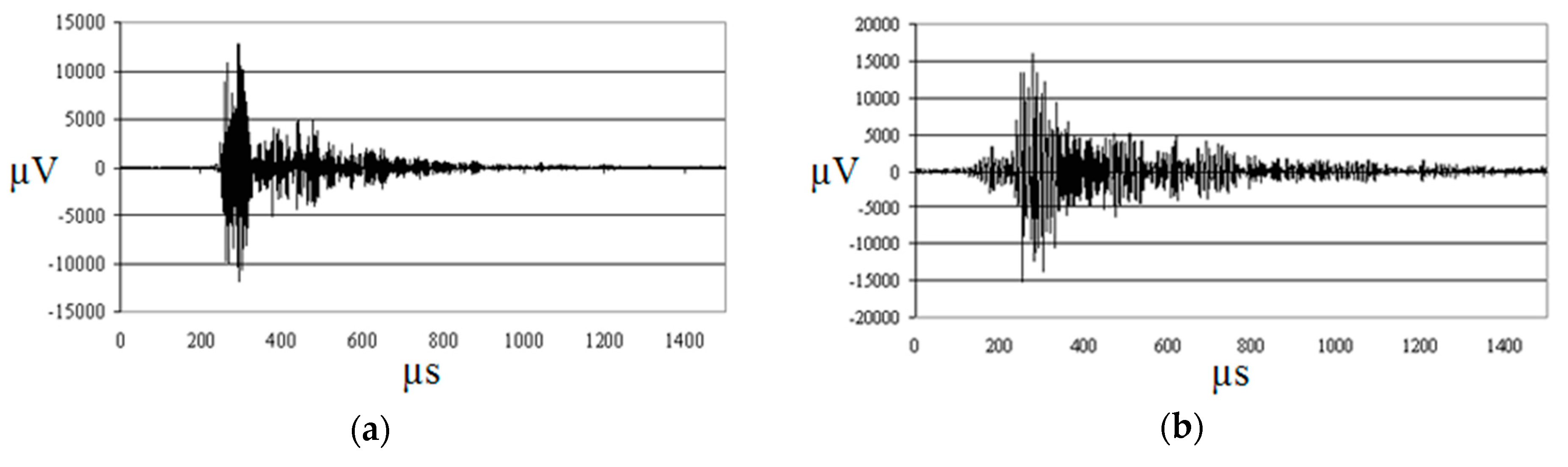
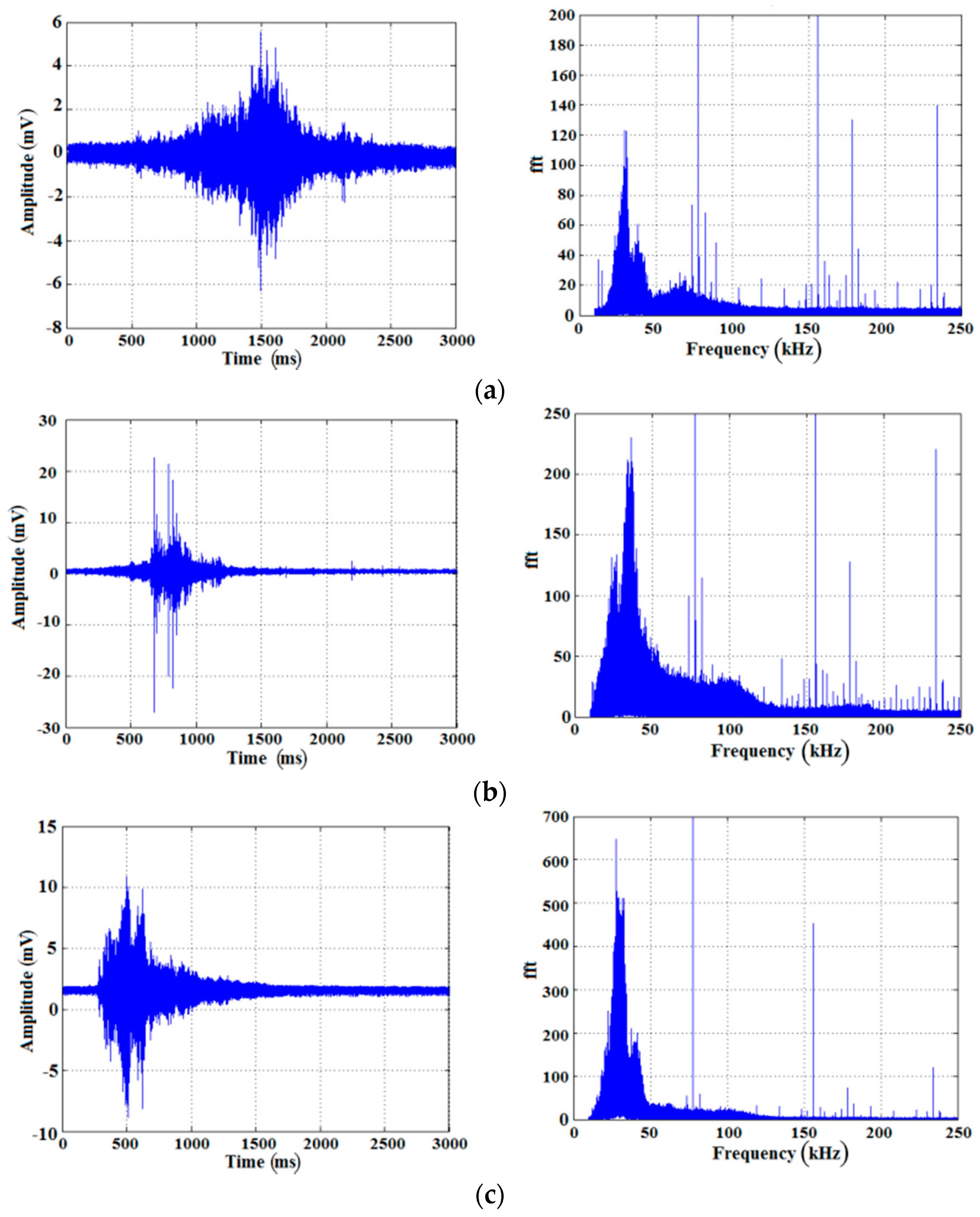
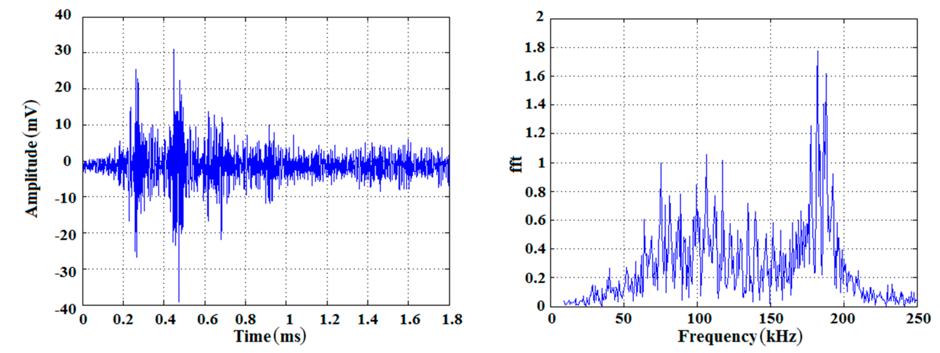
The most representative clusters were formed for signals registered by channels № 8 and № 17 (Figure 3,

Table 1. Parameters of clusters for channels 8 and 17.

Parameters	Channel № 8	Channel № 17
Signals in the cluster	284	138
Mean amplitude, dBAE	72	69
Mean rise time, µs	240	379
Mean duration, µs	893	1057

). These signals had an amplitude of more than 70 dB_AE with a high probability they were generated by AE source located in zone #5.

3.1.3. Testing of the Dismantled Object

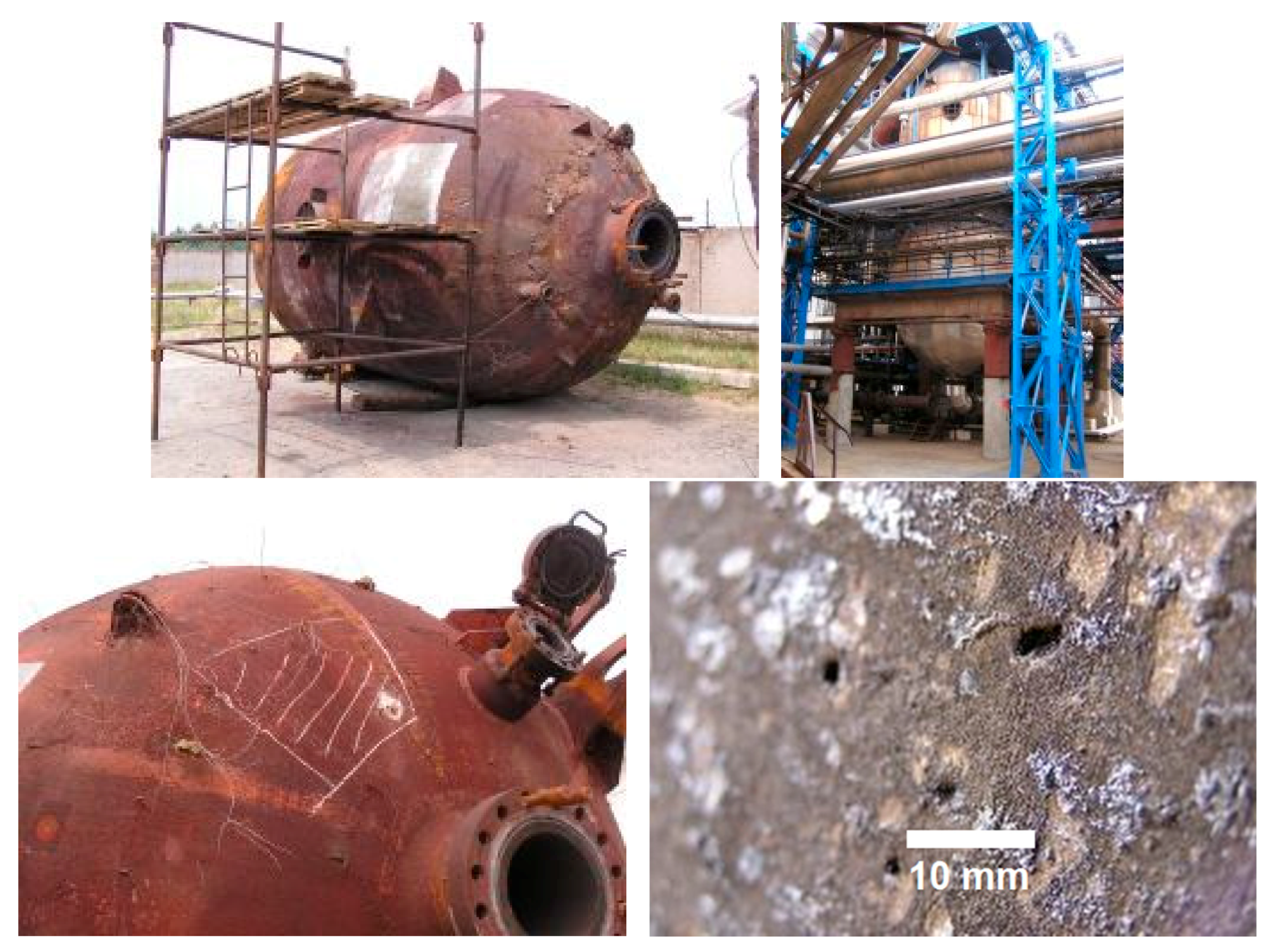
Thus, the results of the cluster analysis confirmed a previously determined degree of danger of AE source located in zone #5. A final decision to stop the hydrotreater was made. The dismantled hydrotreater was investigated by NDT in order to establish the reasons of its transition to the critical state. Internal examination revealed numerous disintegrations of the cladding layer (up to its complete absence in some areas) (Figure 4). Dimensions of damages were up to 5 mm. Ultrasonic testing revealed numerous discontinuities in welds and the base metal shell. The lengths of discontinuities were 100 mm along and 15 mm in depth. In one of the most active zones, discontinuities were detected both in welds and in the heat-affected zone. Certain discontinuities occurred at different depths, from 26 to 80 mm. These damages demonstrated significant degradation with loss of mechanical properties of the metal, which leads to brittle fracture of the structure [11].

Thus, the use of SHM-system allowed, on the one hand, to extend the lifetime of the hydrotreater by 6 months and on the other hand, to prevent the destruction of the hydrotreater during operation with all the ensuing consequences.

3.2. AE Method Application for Bridge Monitoring

3.2.1. Structure Description

Experimental studies were conducted on a highway bridge across a river. It is a 7-span metal bridge with reinforced concrete supports. The foundations for pylons are piled. The length of the bridge is about 700 m. The bridge has 2 traffic lanes. As a result of the abnormal operating impact, the supports #1 and #5 sank in by 112 mm and 44 mm, respectively. After that it was decided to install an SHM-system on this bridge.

Preliminary studies consisted of 3 main stages, the objectives of which were: determination of the AE parameters of noise signals, determination of propagation parameters of the AE signals and determination of the optimal arrangement of the sensors on the bridge construction elements [12,13]. Investigation of the possibility of AE signals detection used Hsu-Nielsen source for location and filtration.

3.2.2. Analysis of Noise Parameters

The first experiment consisted in the recording and analysis of noise at various sections of the bridge. As a data collection system, a 4-channel external USB I/O module “E20-10”, manufactured by “L-Card” company (Moscow, Russia), was used. This system provides the consistently recording data with the sample rate 2.5 MHz for every channel. Two sensors of GT200 type (130–200 kHz) were connected to the module, which were installed on the bridge. The signal from the sensor went to the preamplifier with a gain of 26 dB and a frequency filter of 30–500 kHz.

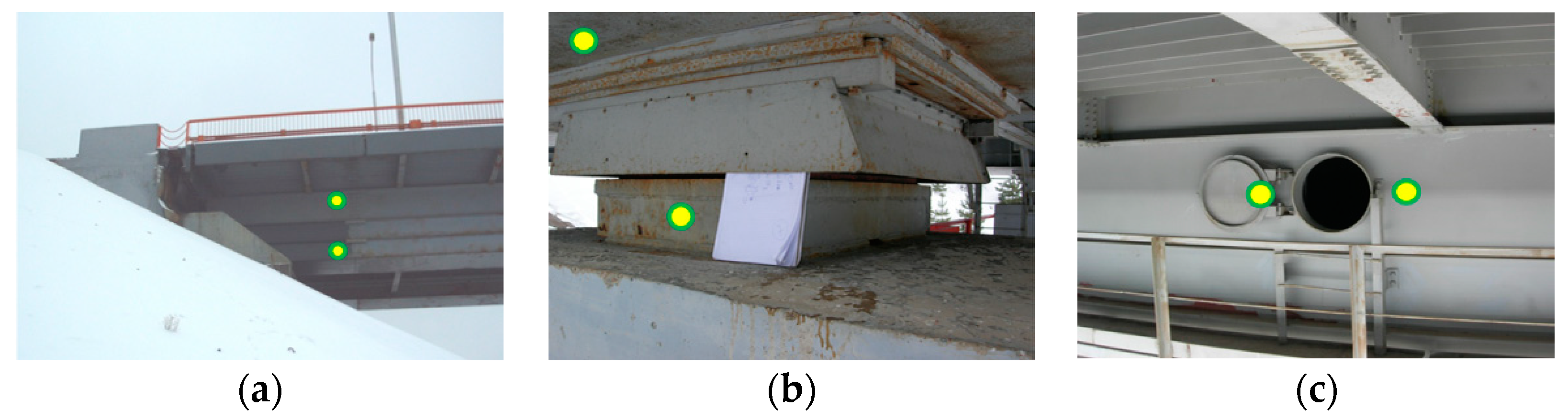
The AE data were taken in 3 different zones of the bridge structure (Figure 5).

Zone I: In the area of the expansion joint near the shore support (Figure 5a), sensors were installed inside the beam structure near the bolted joints. The distance between the sensor and the expansion joint is 5 m. Zone II: In the area of attachment of the beam and the support (Figure 5b), AE sensors were installed on the lower girder and on the support. Zone III: In area of the exit hatch section of the box beam (Figure 5c), AE sensors were installed inside the beam structure at a distance of 3 m from each other symmetrically with respect to the hatch.

For all signals from passing vehicles, the energy is concentrated in the frequency region up to 60 kHz.

Vibration of the bridge from passing vehicles was the most common type of noise (Figure 6). Some characteristic features of these signals are a long duration (1–3 s) and relatively high amplitudes of about 56–90 dB_AE. The primary reason for the appearance of these signals is the fact that the passage of the cars leads to vibration and friction of poorly fixed structural elements.

Signals caused by impacts of structural elements have amplitudes similar to signals from passing vehicles, of the order of 56–90 dB_AE but they have 1–2 times shorter duration, not exceeding 50,000 µs (Figure 7). The energy of the signals, as a rule, lies in the frequency range up to 200 kHz. The primary cause of these signals is the vibration of weakly fixed structural components of the bridge, as a result of which their collision occurs. An example may be the impact of a ladder or hatch on the bridge girder or the impact of wheel sets on the expansion joint [14].

3.2.3. Analysis of AE Signals Propagation

Hsu-Nielsen source was used to estimate signal propagation properties. The measurements in this experiment were carried out using the A-Line 32D system (Interunis-IT) with threshold data acquisition. The ADC sampling frequency was 2 MHz. The following values were obtained: AE wave propagation speed is 2838 m/s, attenuation coefficient in the far field zone is 1.65 dB/m. Based on the obtained values of the attenuation coefficient, noise level and amplitudes of signals from the AE signal simulator, the maximum distance between the AE sensors for linear or planar location was determined. This value lies in the range from 11 to 16 m.

An acoustic contact quality was also estimated in zone II (Figure 5b). In the course of the experiment it was revealed that the signals simulated in the girder region are not detected by the AE sensor mounted on the support, which indicates that there is no acoustic contact. Thus, for a full monitoring of the bridge, separate AE testing of both the supports and the main upper part of the bridge is necessary.

3.2.4. Identification of AE Signals from the Hsu-Nielsen Source

Simulation of AE signals by the Hsu-Nielsen source was carried out at various points of the lateral beam of the bridge structure inside one of the bridge sections. The distance from the sensor to the Hsu-Nielsen source was from 0.15 to 15 m. Totally about 100 pulses were excited (Figure 8).

For detection of signals from the Hsu-Nielsen source, a planar location was constructed (Figure 9). It is revealed that the signals from Hsu-Nielsen source are with certainty located in their actual places and form compact clusters, in contrast to noise. This confirms the possibility of identifying signals from defects based on location data.

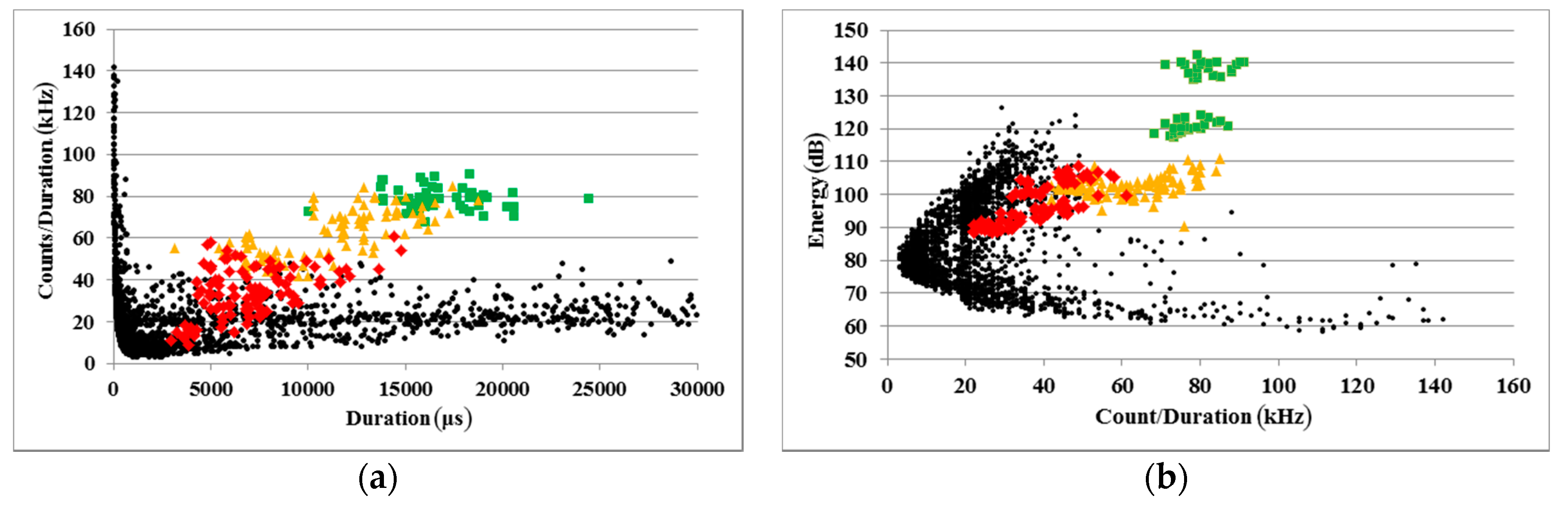
Since the bridge is a structure of testing characterized by a high level of acoustic noise, a locational cluster corresponding to a defect can be masked by a large number of false locations of noise events. The complexity of the detection algorithm lies in the fact that the values of the AE parameters of the noise and useful signals vary in fairly wide and overlapping ranges. This is due to the variety of noise sources and different distances between the sensor and points where the defect or simulator is placed - from 0 to 15 m.

The difference of parameters is best shown in the two-dimensional plots of characteristics, for example, on the scatter plot diagram “Counts/Duration versus Duration” (Figure 10a) and the scatter plot diagram “Energy versus Counts/Duration” (Figure 10b). As can be seen from the chart, the AE impulses emitted at the distance of 7 m from the sensor have the parameter distribution other than the noise distribution. When the distance increases over 7 m, the differences disappear, the AE impulse parameters become close to those of noise [13].

3.2.5. SHM-System

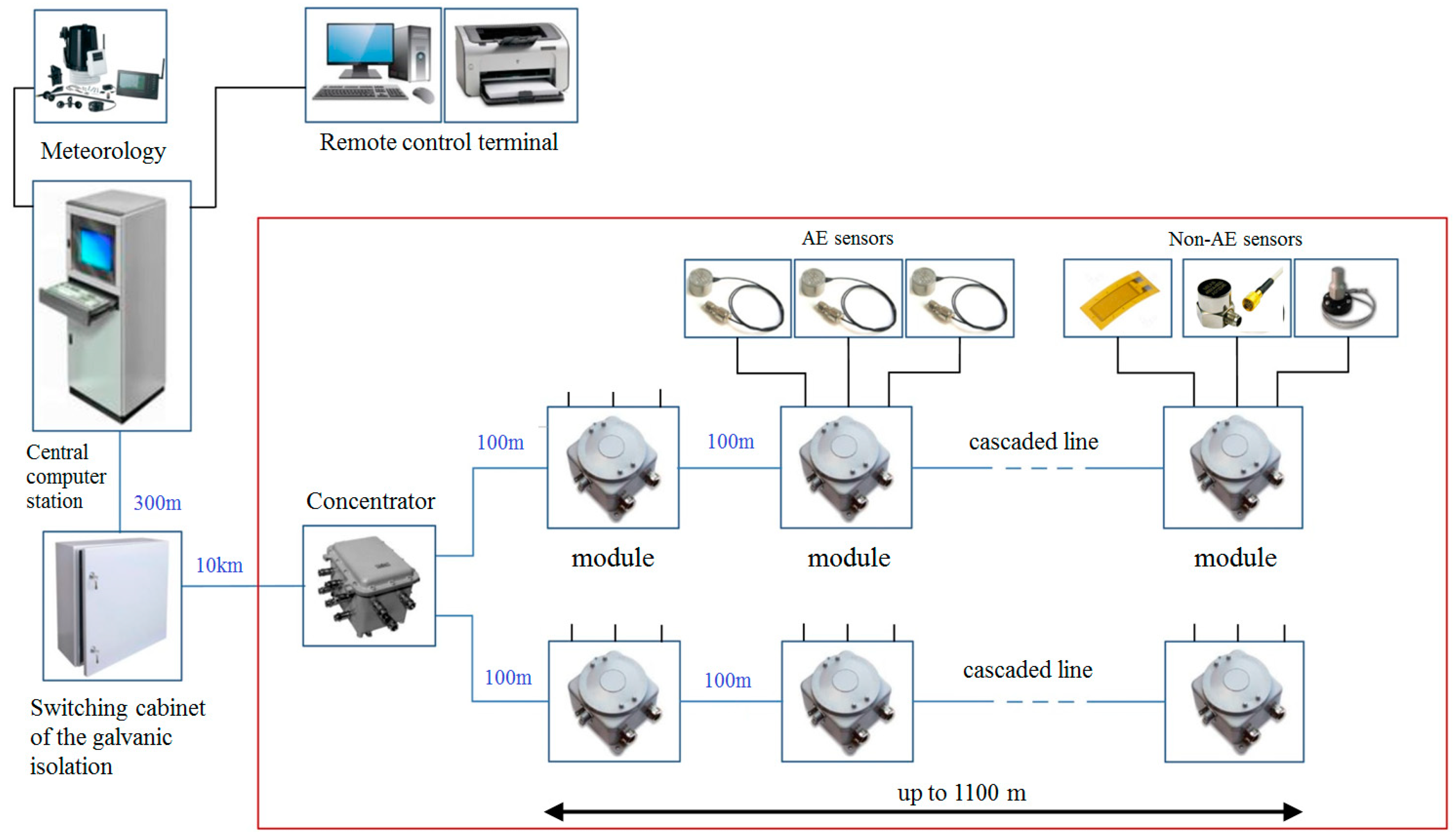
SHM-system for this application was designed and installed on the bridge. AE sensors, vibration transducers, strain gauges, temperature sensors, modules for collecting, measuring and processing signals were installed on the span of the bridge structure (box beams). Low-frequency AE sensors, inclinometers, crack opening sensor were installed on the supports. In addition, SHM-system is equipped with video cameras to monitor the traffic situation, a weather station to monitor wind loads and to determine the presence of precipitation for AE signals filtering and a communication system.

3.3. High-Temperature Process Pipeline

On the active high-temperature pipeline without decommissioning, studies were produced to assess the feasibility of conducting AE monitoring. Application of AE monitoring of high-temperature or cyclic thermal loaded structures is an effective method for defects detection. Several interesting applications are described in the papers [15,16,17,18]. The tested object consisted of pipe sections with a diameter of 50 to 80 mm with a total length of 8 m. Individual pipe sections were connected with both flanged and welded joints. The working medium of the pipeline was molten salt, the temperature of which could reach 600 °C. To synchronize the AE data with the operating mode of the pipeline, one thermocouple was installed. 8 AE sensors were installed through waveguides. Simulations of AE signals were carried out once per day by emitting from a sensor to monitor the attenuation factor.

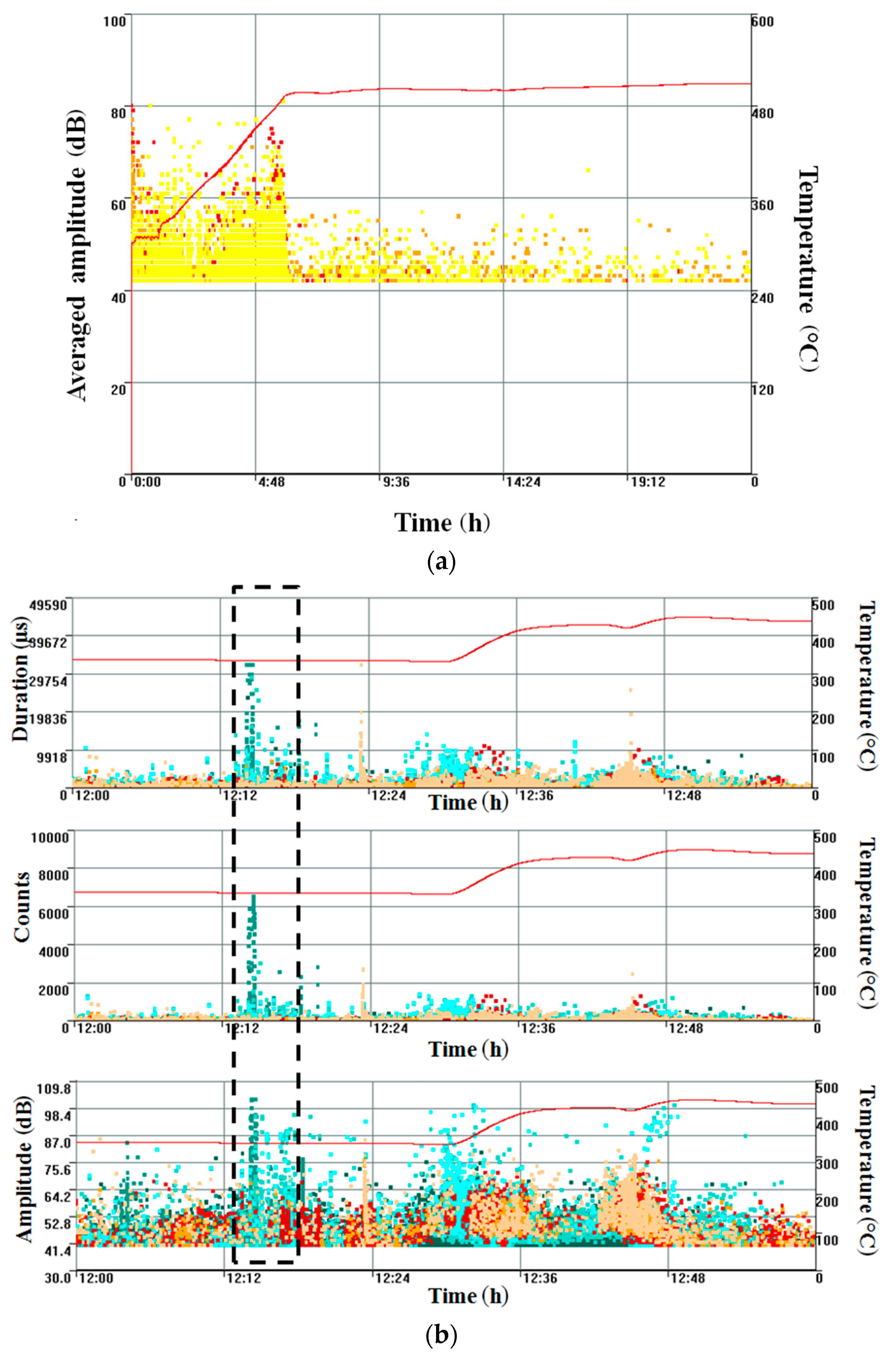
When the pipeline was cold, the propagation velocity and attenuation coefficient were measured, which were 4900 m/s and 1.7–2.7 dB/m, respectively. Then the pipeline was put into operation. AE data were taken in various operating modes of the pipeline for 63 days, including in the total amount for 15.5 days in a stationary high-temperature regime. The process of heating the pipeline was long and took up to several days. During the heating process, the melt began to flow into the pipeline. 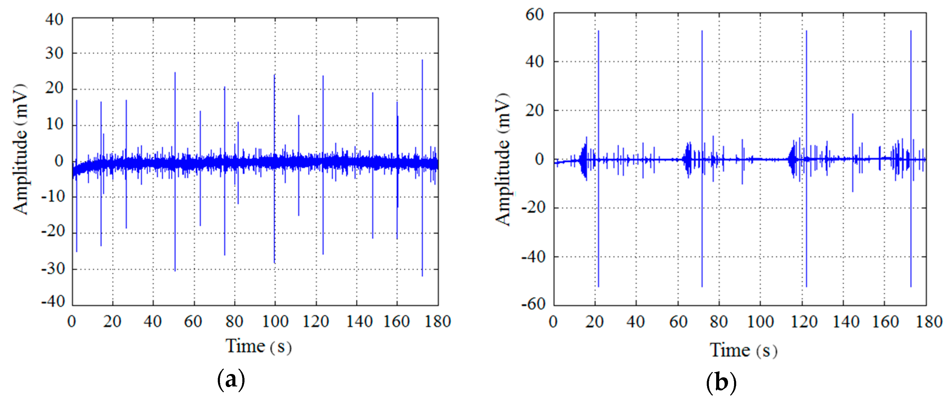The most suitable was the use of the frequency range 100–500 kHz and the threshold in the region of 40–55 dB_AE. It was found that the activity and amplitudes of noise increased significantly with the pipeline temperature rising at a rate exceeding 1 °C/min, especially when clamping fixtures for waveguides were used (Figure 11a). Amplitudes of noise reached values of up to 100 dB_AE. It is assumed that the occurrence of noise is associated with the thermal expansion of the pipeline, which induced friction on the thermocouple and other items on the surface of the pipe. During the work in the stationary mode, the noise level was reduced to an acceptable one and amounted to about 50 dB_AE.

It is revealed that the attenuation coefficient increases with the accumulation of sediments on the inner surface of the pipeline and can reach 58 dB/m. With this level of attenuation, the maximum distance between the AE sensors could not be more than 0.7 m. The value of the propagation velocity for acoustic waves was unchanged.

In the course of the work, the melt leakage was observed as a result of the destruction of the flange joint gasket. In this case, the AE system recorded an increase in the duration of the AE signals a few hours before the leak invisible under the layer of thermal insulation began to be observed visually (Figure 11b).

As a result of the conducted studies, the possibility of AE monitoring of the most critical sections of the pipeline was confirmed: the detection and location of crack-like defects and detection of leaks on this pipeline by the AE method can be accomplished.

3.4. SHM-System for Oil Refinery Equipment with Defects Presence

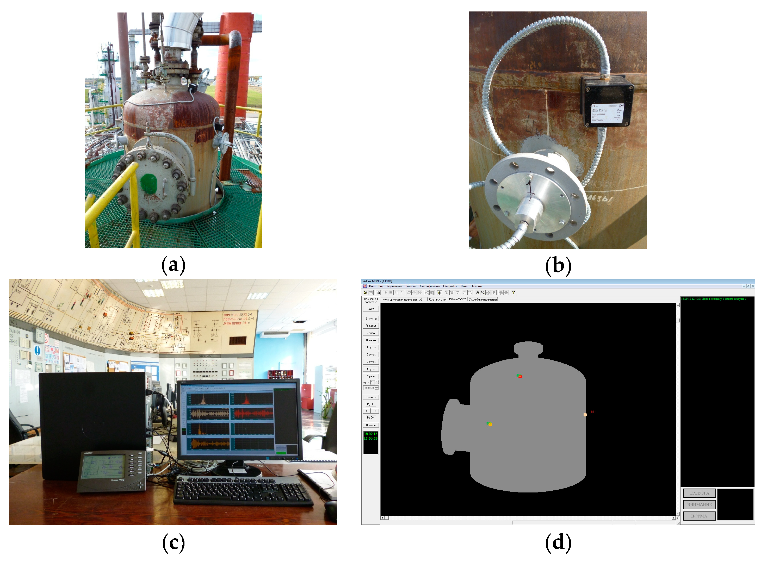
At an oil refinery, non-permissible defects were found in the upper part of the gas adsorber of the circulating gas (commissioned in 1970). From 1999 to 2009, the lamination was known to exist in the main upper end plate (the area of the lamination ~0.4 m², the depth of the lamination: 6.1–12.4 mm). 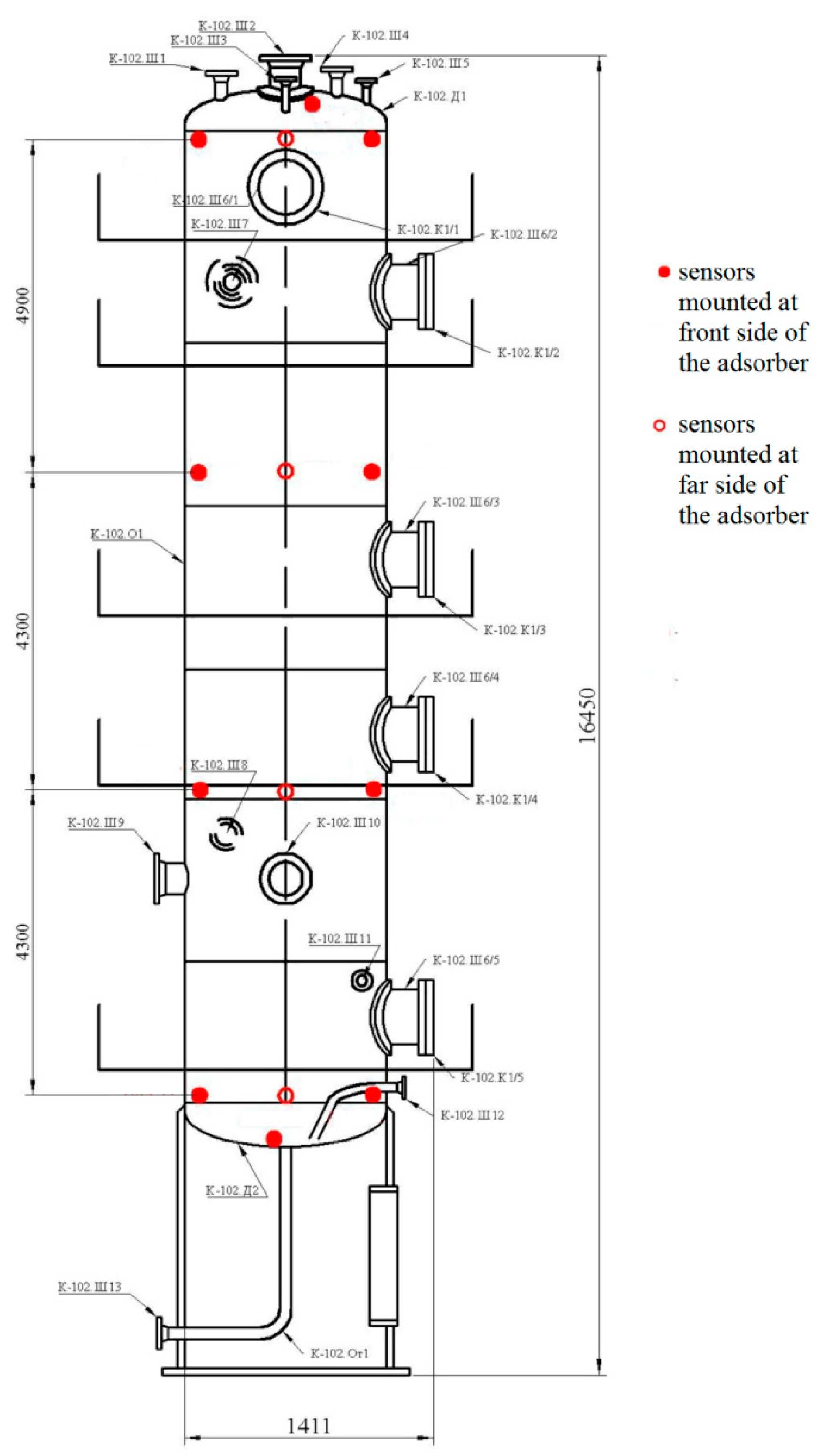On the same unit, the defect of the planar type (crack) in the weld of the shell to the end plate (length: 140 mm, depth: 12–14 mm) was also present (Figure 12). This gas adsorber has the following parameters: working pressure: 4.2 MPa, operating temperature +45 °С, wall thickness: 22.0–24.0 mm, the inner diameter: 1.156 m and the height: 16.45 m.

A preliminary decision was made to install a monitoring system for the upper part of the adsorber. The main task of the monitoring system was to ensure safe operation of the adsorber before its replacement within a year.

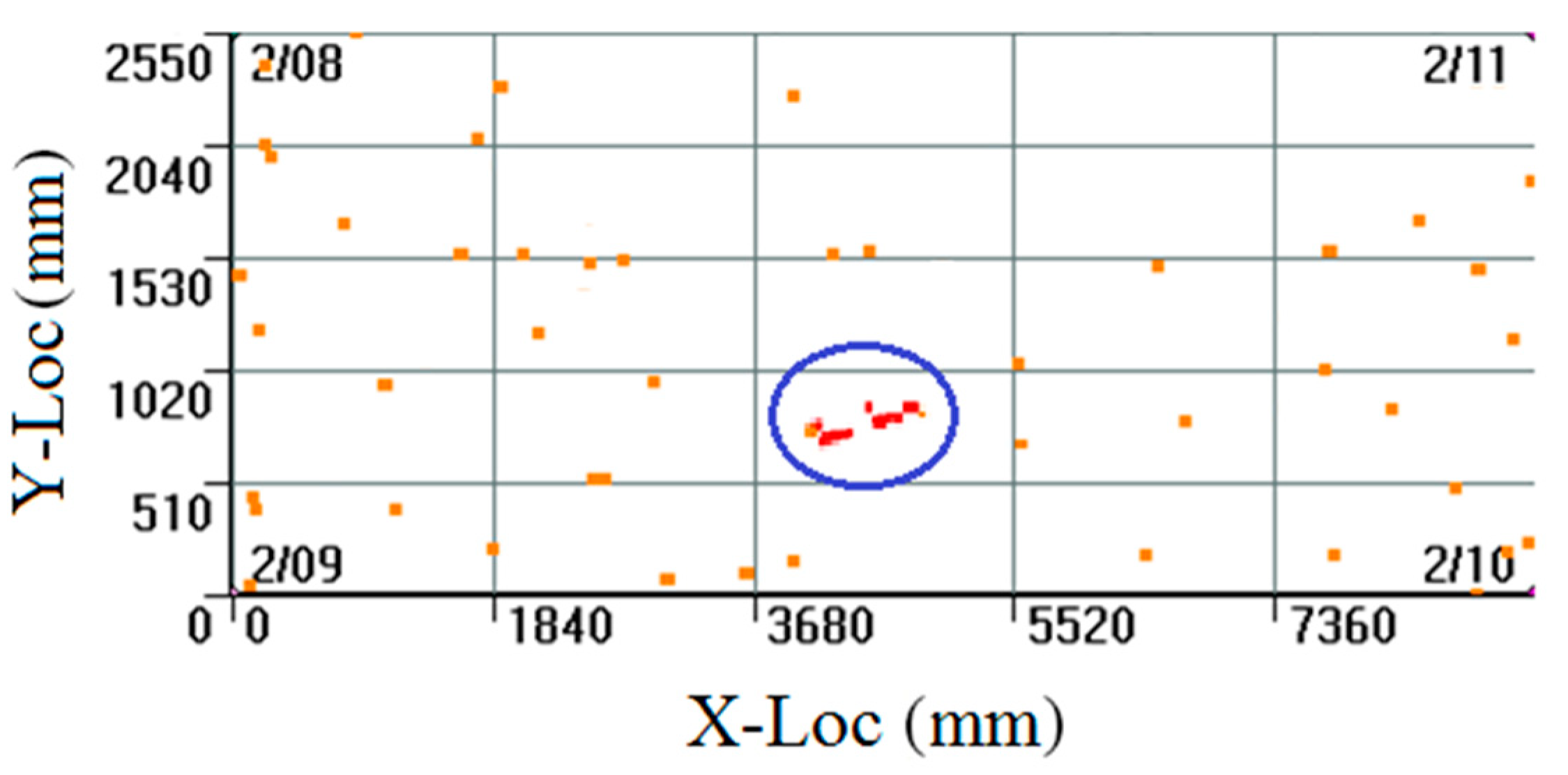
Prior to installation of the monitoring system during the overhaul in the spring of 2012, its AE testing was carried out (Figure 12 and Figure 13). AE sources of class I and II were registered, the locations of which were correlated with the place of previously detected defects on the vessel head of the adsorber (Figure 12). This allowed us to assume the possibility of further expansion of the lamination zone during the life extension period of the adsorber.

Based on the results of the AE testing, the previously approved decision on the installation of the monitoring system for the vessel head of the gas adsorber was confirmed. The expanded SHM-system included 4 AE sensors and a weather station (Figure 14). The threshold data acquisition approach was used, and the threshold value was about 45 dB_AE.

3.5. Roller Bearings of Rotary kilns

3.5.1. Tested Object

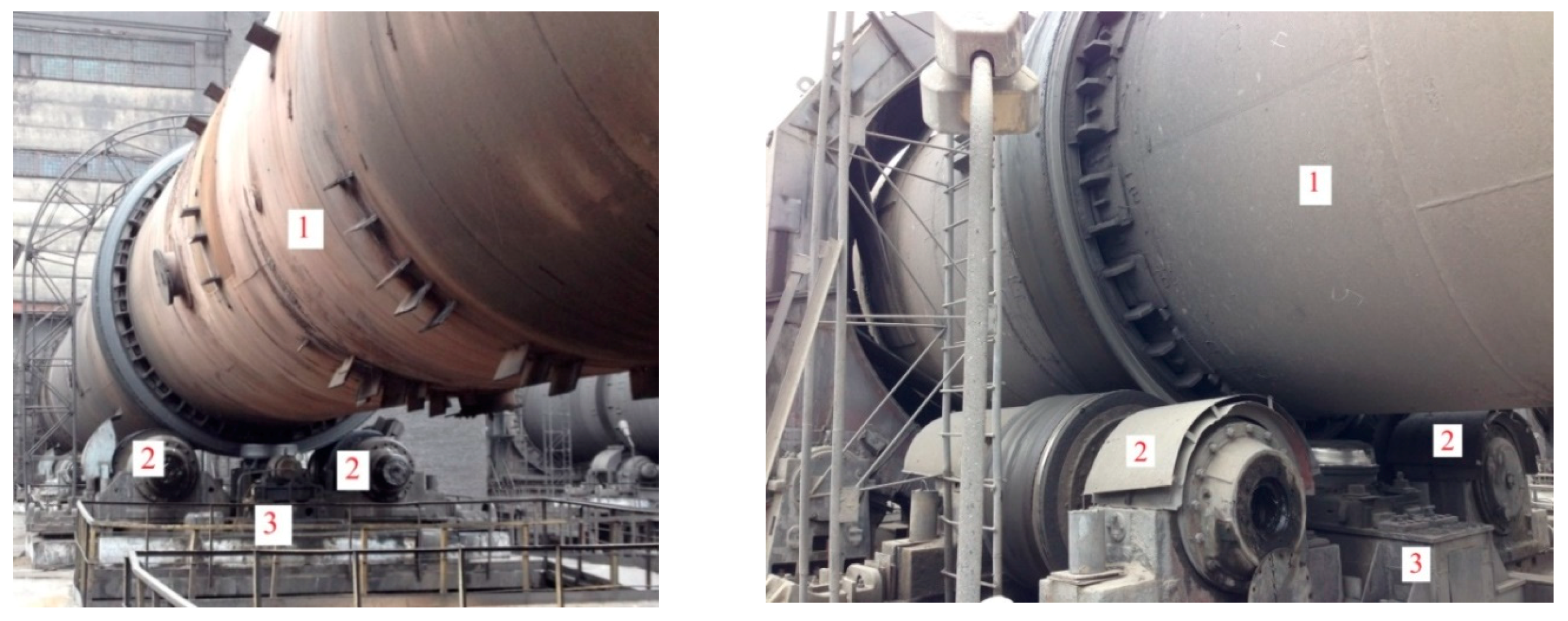
The possibility of conducting AE testing of roller bearings of rotary kilns without their decommissioning was investigated (Figure 15). Using AE monitoring for rotating equipment is an alternative solution to vibrodiagnostics [19,20]. In the case of slowly rotating elements, the use of the AE method is more effective for the diagnosis of rolling bearings, rotating shafts, rollers and others [21,22]. Experimental work was carried out at an alumina plant in the sintering and calcination shops and also in the repair shop.

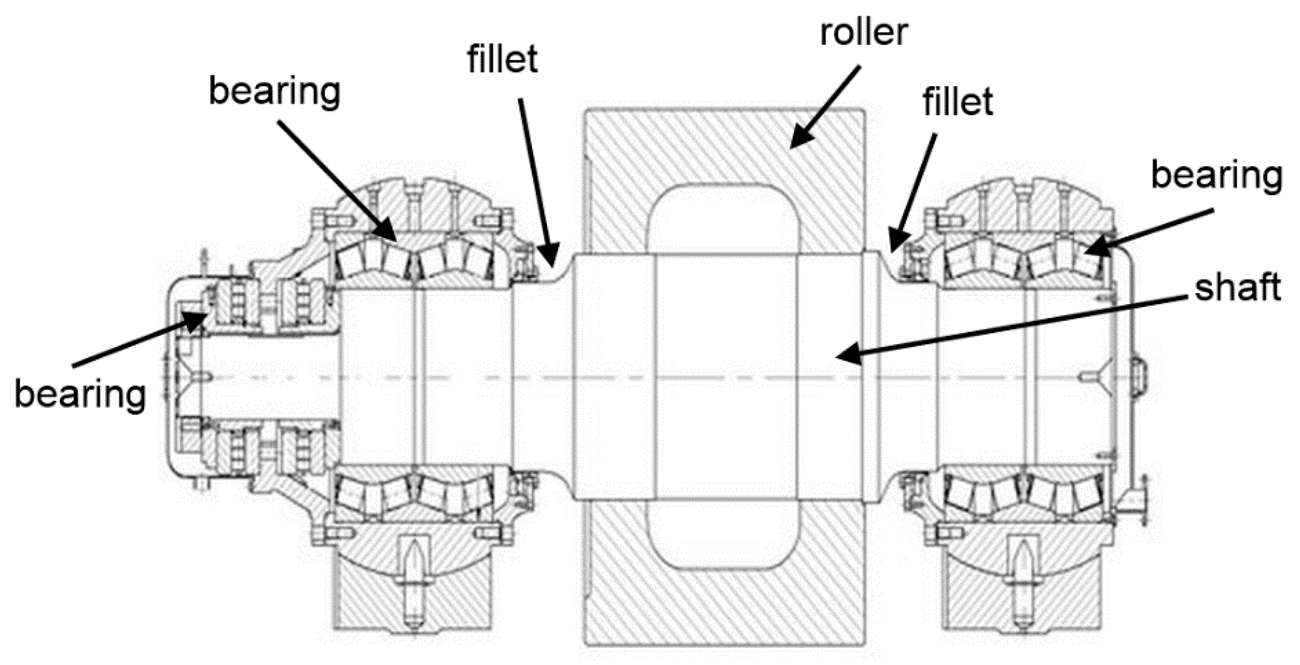
The kiln is a cylinder with a diameter of up to 5 m and a length of up to 185 m, installed with a slope. The kiln is supported by 7–8 pairs of roller bearings. Each pair of roller bearings consists of 2 support blocks, mounted on a common foundation. Each block consists of a shaft pressed onto it by a supporting roller and 3 bearing assemblies mounted in 2 bearing housings (Figure 16). The rotation period of the kiln is 50 s; the rotation period of the support roller is 12.5 s. The lifetime of the monitored supports was from 1 to 13 years.

Roller support is a complex load carrying element of the kiln. In case of its breakdown, an emergency stop of the equipment occurs, followed by the replacement of defective components. Of the 200 supporting blocks at the plant, on average 5 blocks per year are replaced because of broken bearings and 1 more block due to the fracture of the shaft. Therefore, it is necessary to ensure the detection of defects of all its elements such as shaft, roller and bearings.

The roller is a part of the support block and is in direct contact with the kiln. Thus, the main defects on it are scoring and metal chipping from rolling contact under load.

The shaft is a cast steel component. Since roller bearings are operated under unfavorable temperature conditions, with a high level of vibration and under cyclic loading, the most likely defect of the shaft is the formation of fatigue cracks. Since the shaft is a monolithic all steel construction with numerous protrusions and thickness differences, it is difficult to carry out the NDT of shaft by traditional scanning methods, even for roller bearings in decommissioned state. The main bearing elements include an outer ring, an inner ring, cylindrical rolling bodies and a separator. Destruction of the bearing occurs for 3 main reasons: incorrect mounting of the bearing, insufficient quantity or low quality of lubricants, as well as fatigue failure of the bearing. Due to the low angular velocity (1 rotation in 12.5 s), a well-known method of vibrometry is not quite suitable for testing the roller bearings and AE is expected to provide a good solution.

3.5.2. Preliminary Research

AE sensors GT200 was used with a working frequency range of 130–200 kHz. The signal from the sensor was fed to the preamplifier with a gain of 26 dB and a frequency filter of 30–500 kHz. As a data collection system, a 4-channel external USB I/O module "E20-10,” manufactured by “L-Card” company (Moscow, Russia), was used. The output data of this module was long time waveforms of the AE signal with a sampling frequency of 2.5 MHz.

3.5.3. Noise Investigation

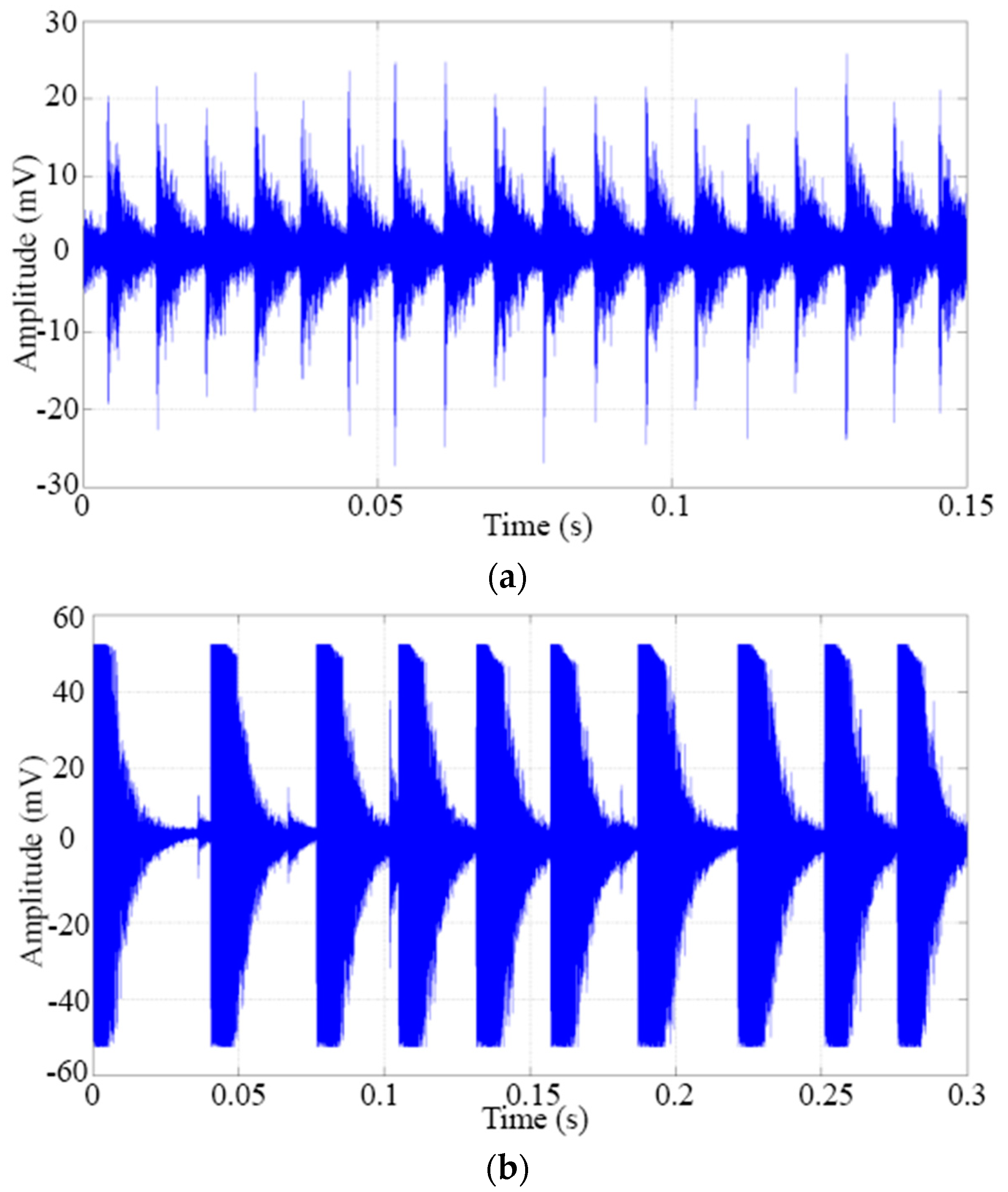
In the case of roller bearings of a rotary kiln in the operating mode, the noise level in the audible range is quite high. However, in the range above 30 kHz, due to the point dry contact between the shroud of the kiln and the roller, the acoustic noise, as a rule, was no more than 32 dB_AE at the most unfavorable point of the structure: at the feed point of the batch. The only significant external source of acoustic noise is scoring and roughness on the surface of the roller or kiln bandage. When it touches the place of scuffing, an AE signal with amplitude of up to 100 dB_AE arises. However, such noise signals can easily be excluded from further analysis, since their registration occurs with a certain period equal to the period of rotation of the roller support, or the kiln (Figure 17).

3.5.4. Calibration Measurements

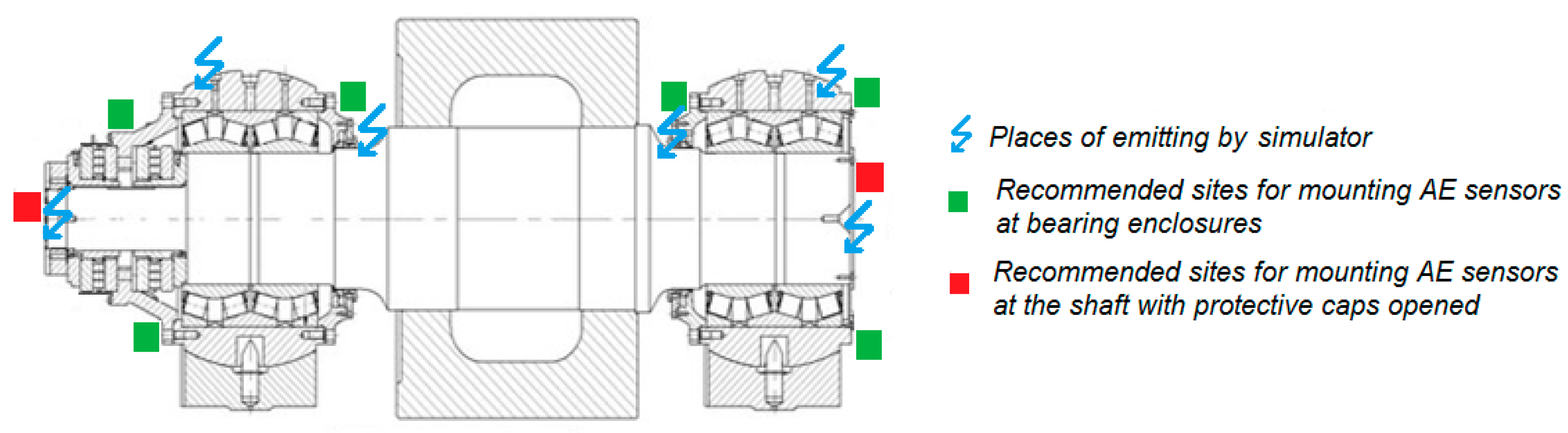
In the repair shop, measurements were made to determine attenuation and propagation velocity of the acoustic signal on the decommissioned support block with the end caps removed. To simulate the sources of AE, an electronic simulator was used. The emission was produced on the shaft in the region of the fillet and at the ends of the shaft, as well as on the inner and outer rings of the bearings (Figure 18).

Within the shaft, the attenuation coefficient was 5 dB/m. The presence of a high attenuation value (30–35 dB) is revealed at the boundary between bearing housings and the shaft.

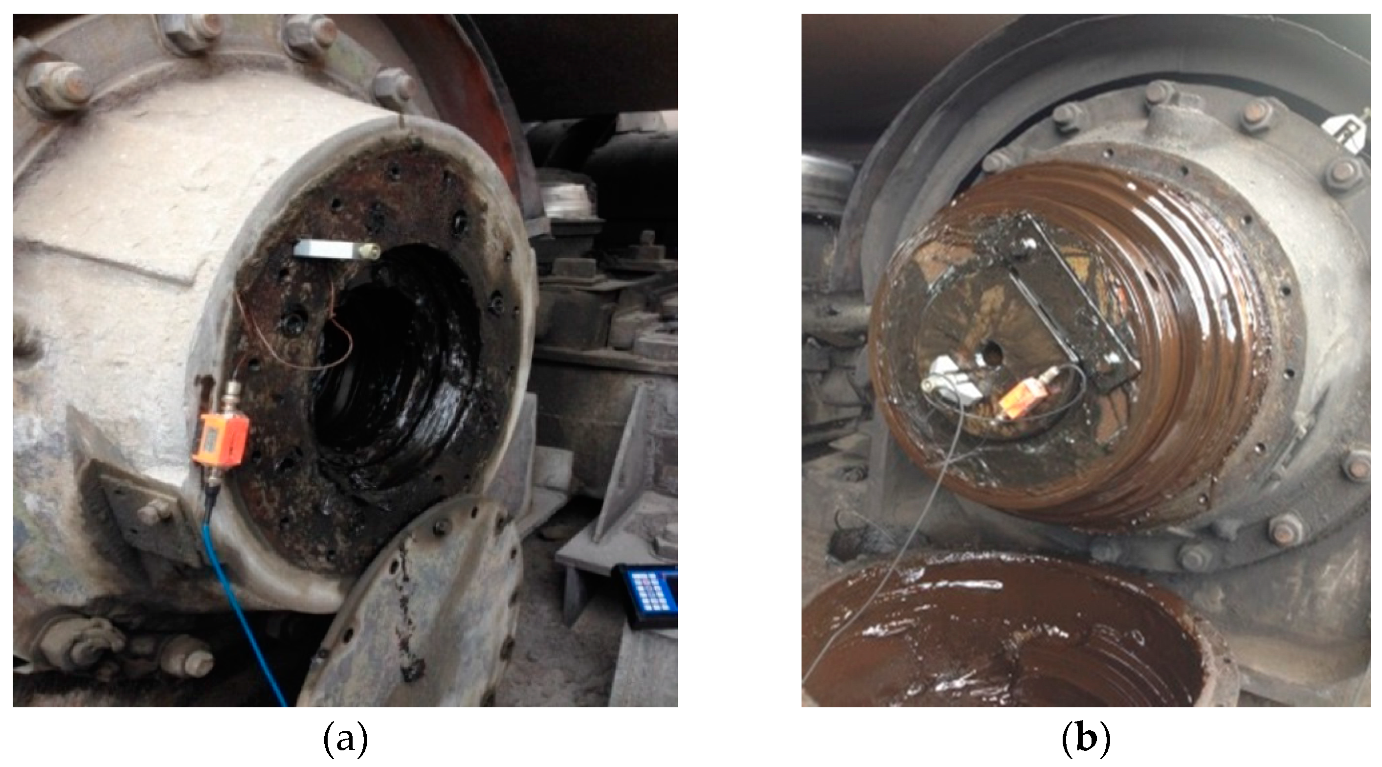
The obtained results revealed that the AE testing should be performed as follows (Figure 18). For full AE testing of all 3 bearings, use the zone location with the accuracy of the element of a specific bearing. For this task, it is required to place the AE sensors at all available access points, namely 3 sensors on each of the 2 bearing housings (Figure 19a). Since the length of the shaft is small (4050 mm), it is enough to provide access to the shaft by removing the covers and to install one sensor at each of 2 ends (Figure 19b) for its full AE testing including linear location. Slow rotation of the sensor at the shaft ends does not cause significant technical difficulties with the duration of the AE testing of about 1 h.

3.5.5. AE Testing

The next stage of the work is to carry out AE testing of the support without taking the object out of operation. The AE data were taken with a regular rotation of the kiln and the support for 1–2 h. Five support blocks with open caps were examined, where both the bearings and the shaft were directly accessible. Also, 10 support blocks with closed caps were tested, where access was available only to the bearings.

3.5.6. AE Testing of Bearings

In one of the bearings, the lubricant dried, which led to intense friction and a rattling in the audible range. AE sensors also recorded signals with an amplitude of about 100 dB_AE and a duration of more than 100,000 µs (Figure 20).

When defects are formed, for example, fatigue cracking or crack, a significant change in the nature of the AE signal flow occurs such as the activity grows, amplitude trends appear, and, most importantly, there is a periodicity of appearance due to the fact that acoustic signals at this stage occur during periodic collision of the bearing roller with place of damage [23].

A moderately active source of AE was detected on the bearing of one of the supports (Figure 21a), which, due to a low characteristic amplitude level, did not undergo the confirmation procedure. A more powerful periodic source of AE (about 100 dB_AE), found on another support (Figure 21b), was a crack in the outer ring of the bearing.

3.5.7. AE Testing of the Shaft

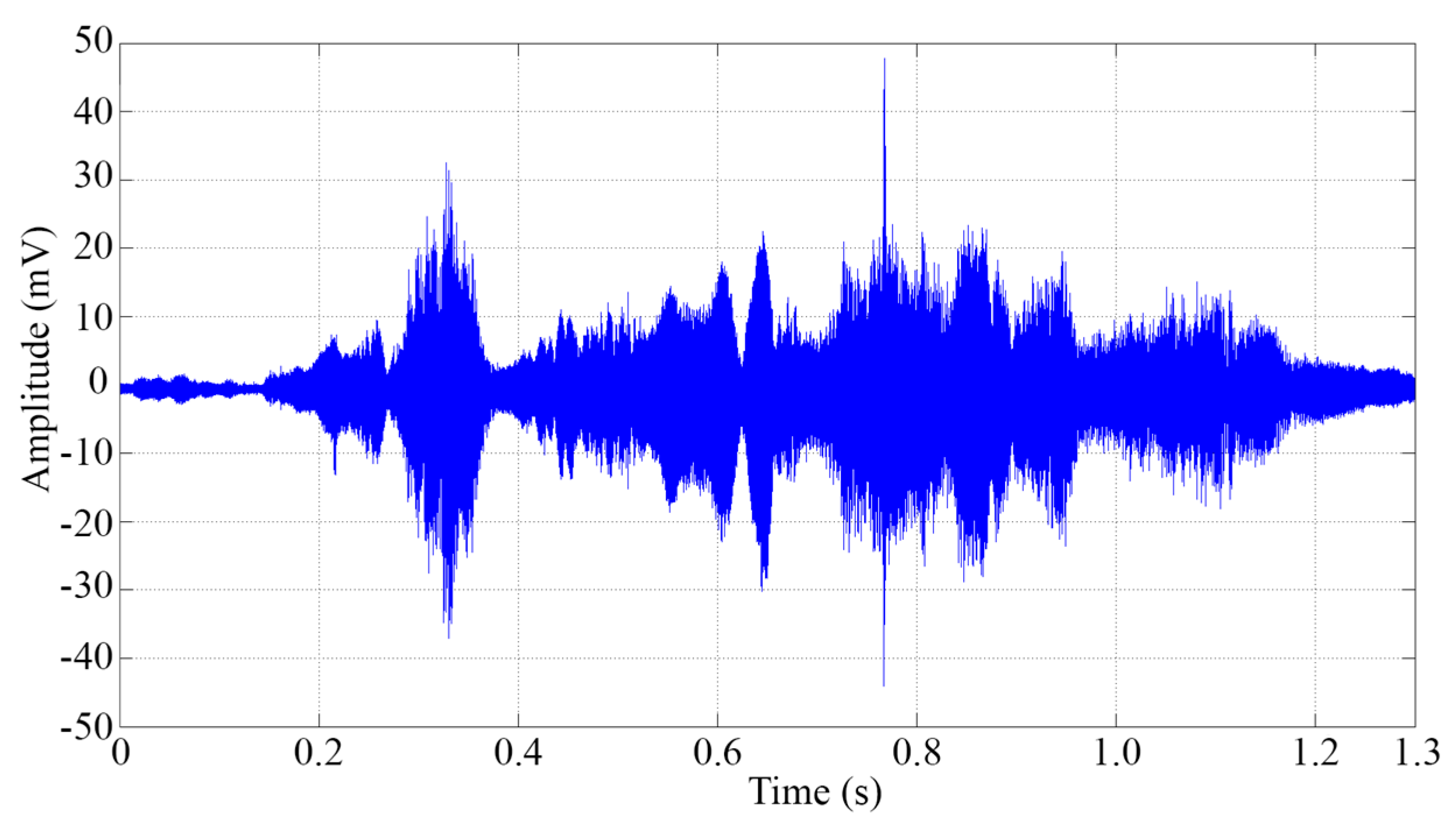
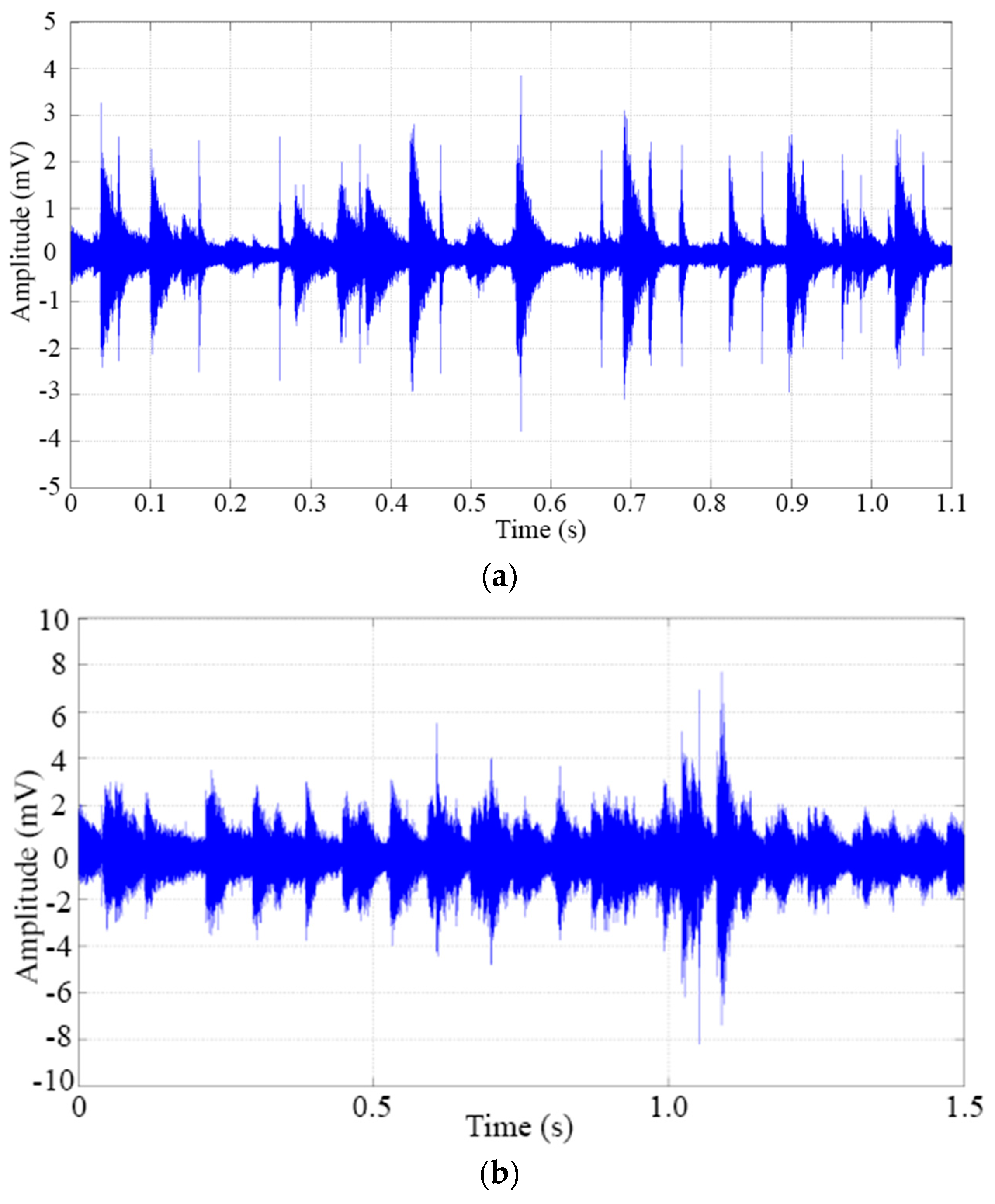
The AE signal, characteristic for the friction process, is a continuous random process characterized by a distribution of pulse amplitudes close to normal, which is not typical for cracks. It is found that higher RMS amplitudes of the acoustic signal are observed in roller bearings with a long service life, which allows us to conclude that the RMS amplitude of the AE signal characterizes the integral degree of wear of the shaft surface [24]. 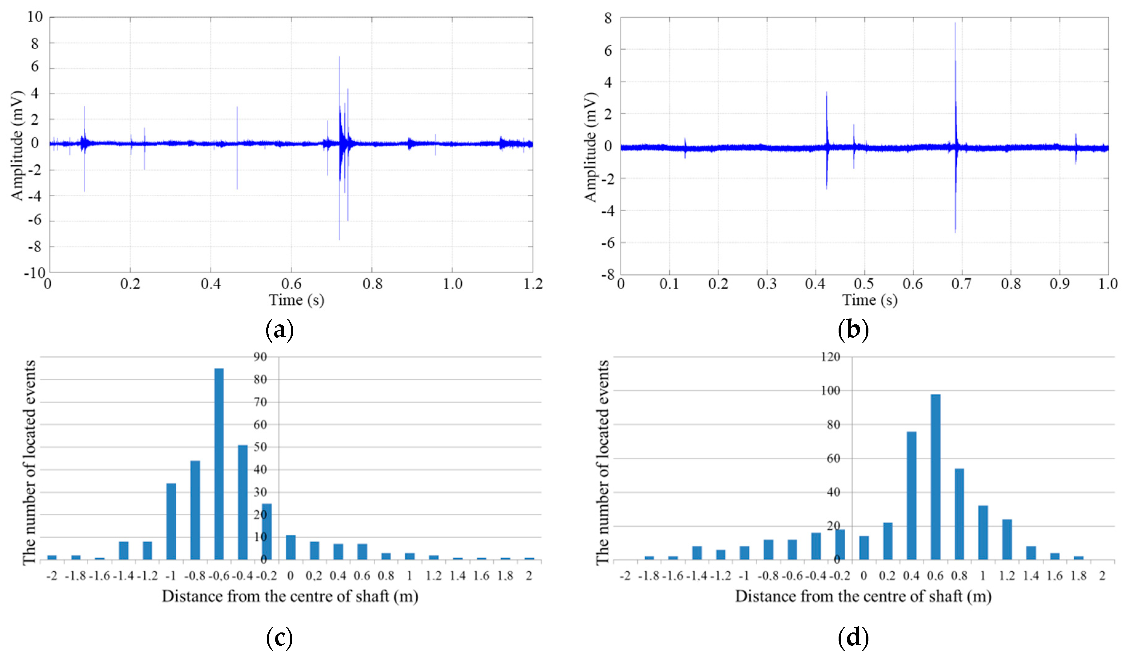Figure 22 shows the signals obtained in the diagnosis of roller shafts that were in service for 2 and 9 years. The corresponding RMS amplitudes are 0.9 mV and 2.2 mV.

The appearance of individual pulses of large amplitude (up to 81 dB_AE) against the background of a continuous signal may indicate the beginning of the destruction of the surface of the shaft in the support block during frictional contact (Figure 23).

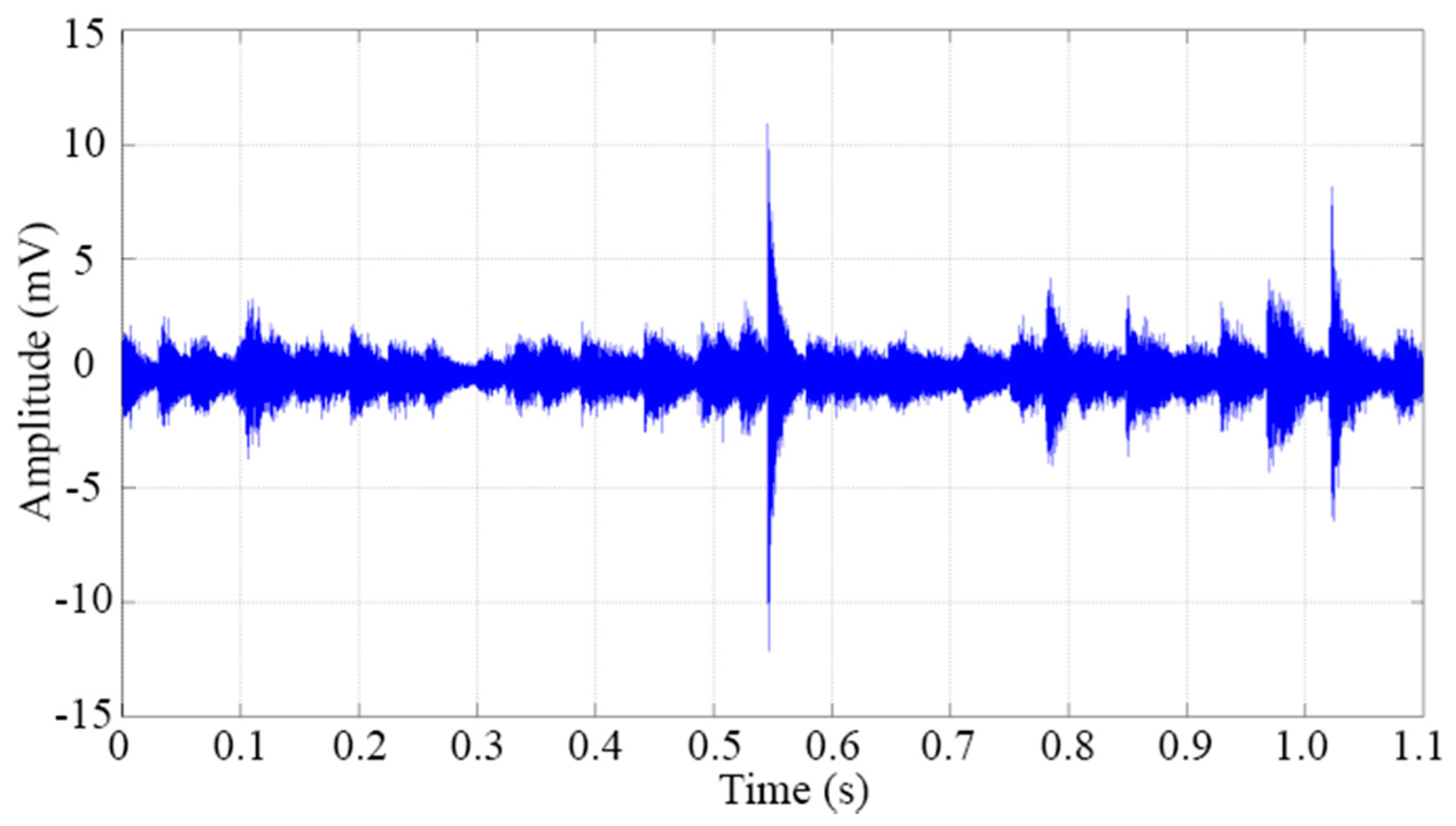
Acoustic emission that is caused by the formation and growth of cracks has a fundamentally discrete and aperiodic nature. When the crack grows, as a rule, high-amplitude signals are generated, with a certain characteristic distribution of the parameters of the AE data stream. AE testing of the support blocks on 2 shafts being in operation for 11 and 13 years revealed AE sources with amplitudes up to 78 dB_AE and activity of about 10–20 s⁻¹ (Figure 24), which, judging from the waveforms and the distribution of the AE parameters, correspond to active fatigue cracks. Analysis of the linear location showed that the sources of AE are located in the region of the fillets, that is in places with the greatest concentration of stresses. The identified sources of AE turned out to belong to the I and II hazard classes and for this reason did not undergo the confirmation procedure.

At present, the design of SHM-system for the roller bearings testing is under consideration.

3.6. Dragline Excavator

On the territory of Russia, handling equipment is often used in difficult climatic conditions. Fluctuations of the temperature, cyclic operating loads lead to the nucleation and propagation of the defects in a load-carrying structure component, which reduces its residual life and, as a result, can lead to an emergency destruction of the structure.

Using AE monitoring can prevent a sudden occurrence of an accident, reduce economic damage and prevent human casualties. Despite the fact that the operation of the lifting equipment is accompanied by a high level of acoustic noise, AE monitoring is possible by optimizing the location of the sensors and applying special methods of data processing [25,26].

Studies were conducted to assess the feasibility of developing an AE monitoring of metal structural elements of a walking dragline excavator. The work of such dragline excavator is carried out all year round, continuously in 3 shifts. Most of the dragline excavators on the mine where the studies were conducted worked out their normal service life; however, it continues to be actively used.

The most stressed and, as a consequence, the most susceptible to the formation of defects are the struts. Emergency situations with dragline excavator lead to downtime, whose duration, for example, in 2016 at one mine was 812 h. Currently, in accordance with the recommendations of manufacturers two times a year periodic diagnostic tests of dragline excavator by ultrasonic method are performed.

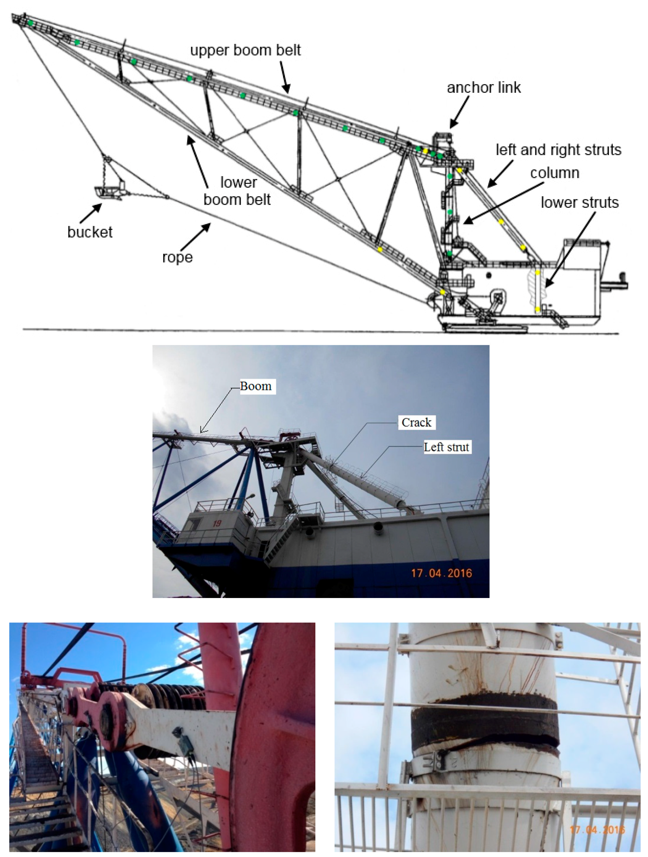
Research work was carried out on booms and struts of dragline with bucket capacity—20 m³ and boom length—90 m, which previously had damage at the left strut near the weld (Figure 25). The work was carried out without dragline excavator decommissioning. A 30-channel A-Line DDM AE system and GT200 AE sensors with a working frequency range of 130–200 kHz were used. A-Line DDM system provides the principle of digital data transmission. The system consists of several sequentially connected measuring lines. The amplification of AE signals, filtering, AD conversion and threshold impulse detection and calculation of AE parameters are carried out in the AE module, which is located next to the AE sensor directly in the tested structure. AE sensors were installed on the main structural elements of the dragline: 3 on the left and right struts, 8 on the upper boom belt and 4 on the lower boom belt, 4 on the lower struts and 3 on the column. The distances between the AE sensors were from 5 to 15 m. In addition, 5 AE sensors were mounted on the anchor links where the zone location was carried out, since they consist of structural elements between which there is no acoustic contact. AE monitoring of a rope was not carried out, as the damage to the rope does not lead to prolonged downtime. In addition, the rope is a movable part, that greatly complicates its AE testing. Data was collected directly during the work of the dragline.

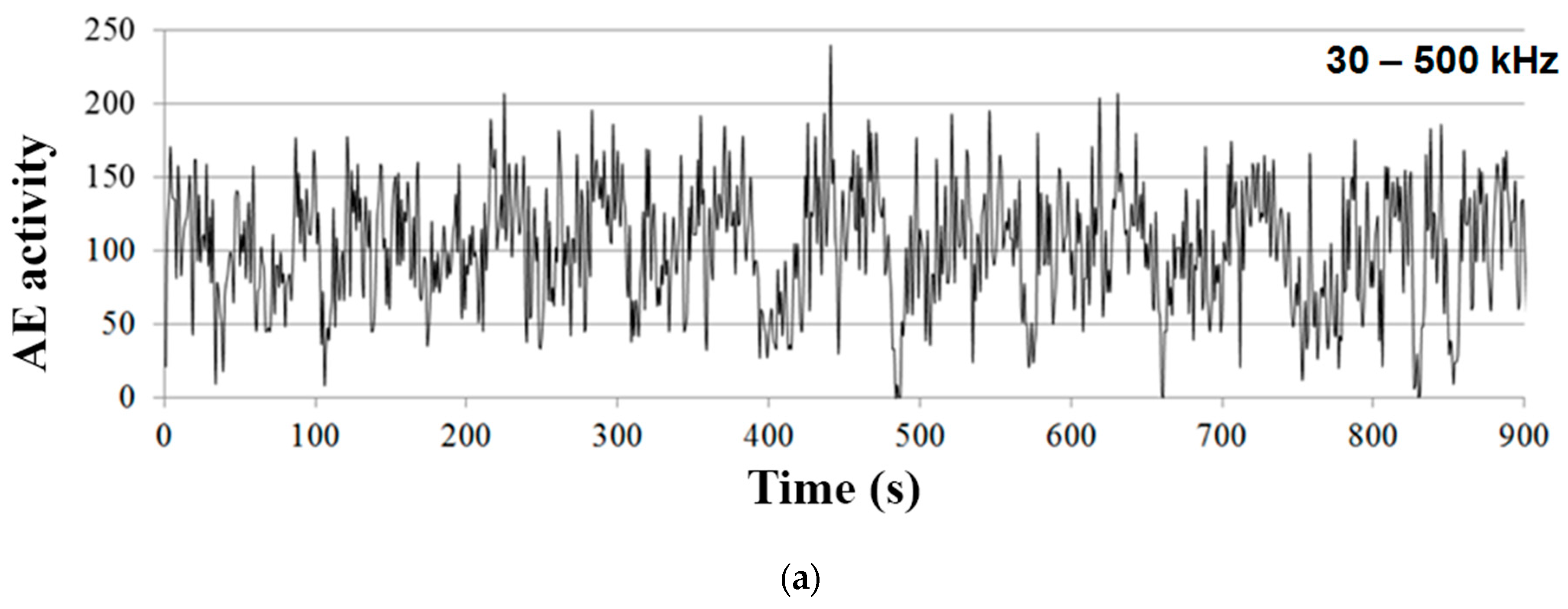
At the first stage, the frequency range and threshold were selected and the acoustic properties of the monitored object were determined. Two frequency ranges were tested: 30–500 and 150–500 kHz. When using a wide frequency range (30–500 kHz), an extremely high AE activity was observed, which did not have a visible dependence on the operating mode of the dragline excavator, that is, on the value of the load. Such noise is associated with the continuous operation of the equipment (working winch, loose structural elements, engine operation, vibration, etc.).

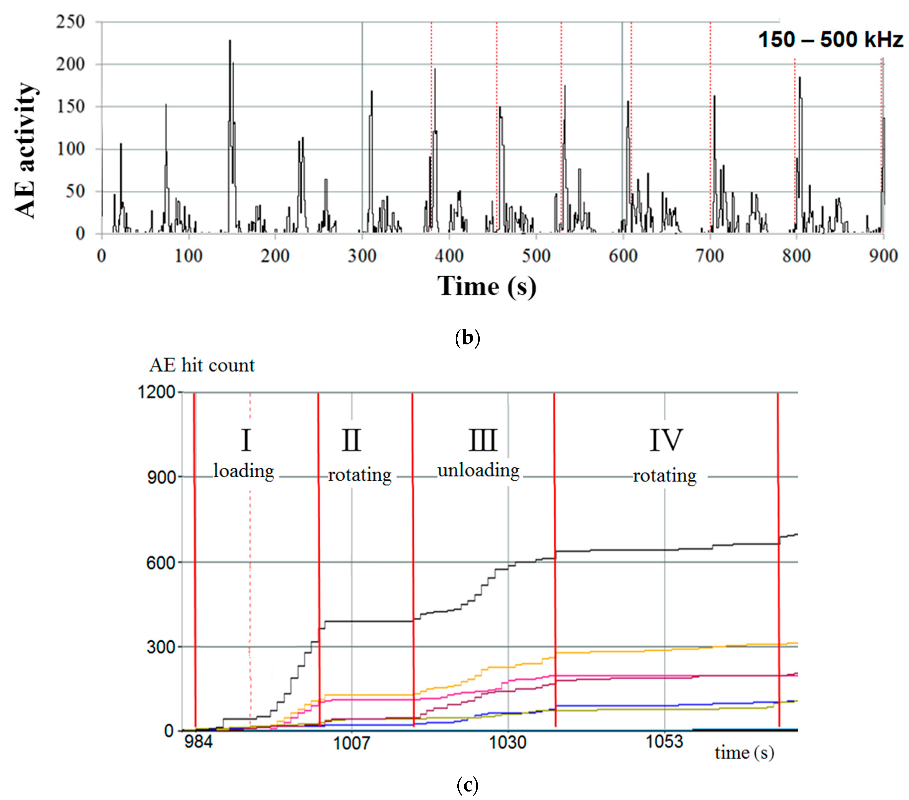
Therefore, a filter of 150–500 kHz was used. Complete noise detuning by the threshold method was still impossible, since the noise reached 100 dB_AE. As a compromise, a threshold value of 50 dB_AE was chosen. With such settings, the nature of AE activity became synchronized with the cycle of operation of the dragline excavator (Figure 26). The greatest activity was observed with excavation of the ground and with unloading the bucket, that is at the loading of the structure, when cracks could grow and at structure unloading, when the crack edges can rub each other.

Measurement of the acoustic properties of the monitored excavator was carried out using the Hsu-Nielsen source. The following values were obtained: velocity was 3200–3700 m/s and attenuation was 1.5–2.8 dB/s. The recommended maximum distances between AE sensors that ensure a linear location are from 4.5 to 9 m.

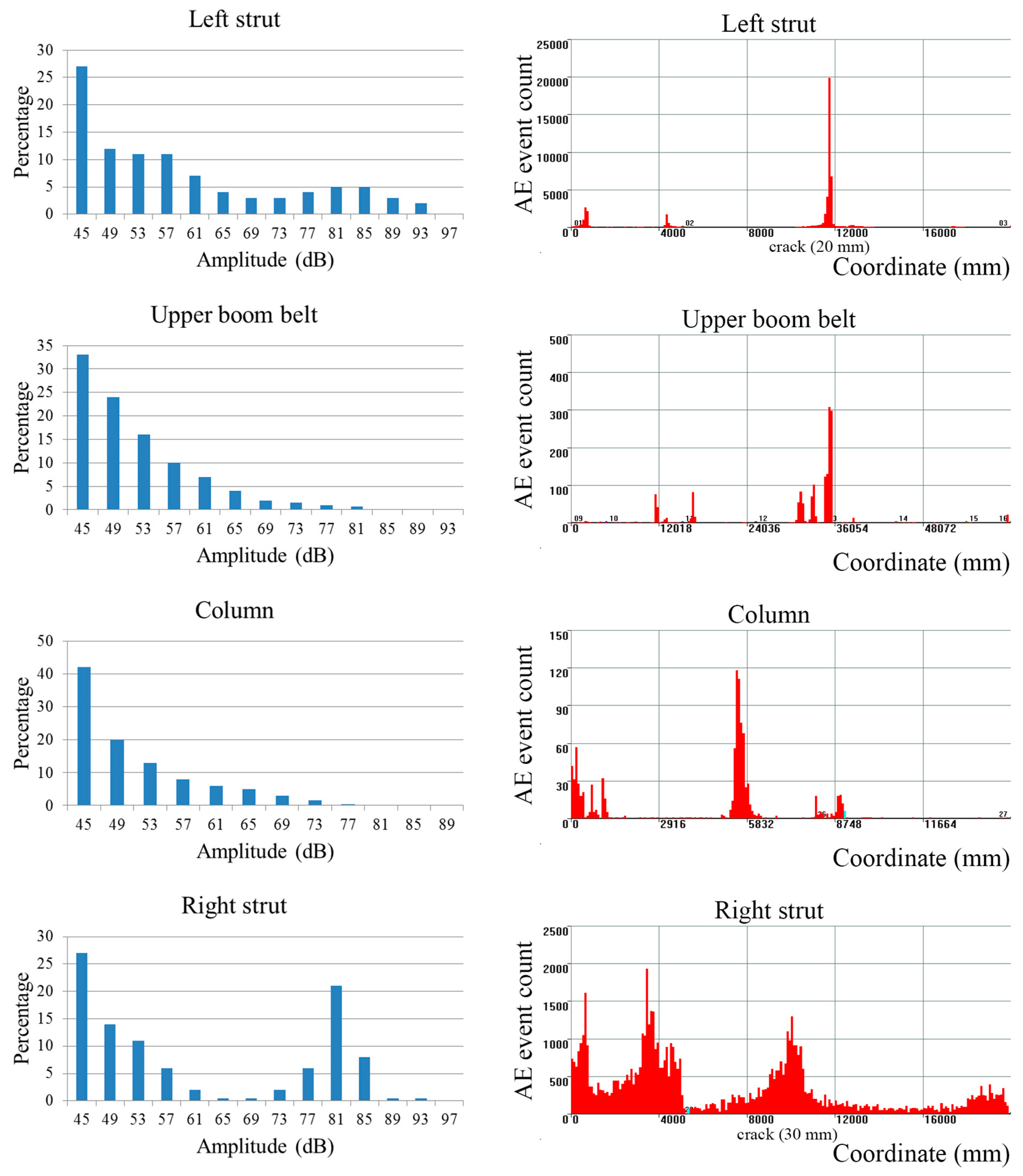
At the second stage, within 2 days, the AE data was collected directly for subsequent detailed analysis. The distribution of the AE signal amplitudes was analyzed. For all structural elements except for the struts, the differential distribution of the amplitudes was exponential, that is corresponding to a random noise process. On the left and right struts in the range of amplitude values of 80–85 dB_AE, the distribution was significantly different from the exponential, which indirectly indicated the presence of a defect.

The results of linear location analysis were as follows (Figure 27). On the lower boom belt, there were no sources of AE. Several sources were found on the column and the upper boom belt, which turned out to be noise, since they were localized near the winch attachment points, or were inactive. On the left and right struts, a linear location revealed 3 sources of AE on each, near which there were no potential sources of noise. Signals appeared at the stages of loading and unloading. The amplitude distributions presented above also make it possible to classify these sources as defects.

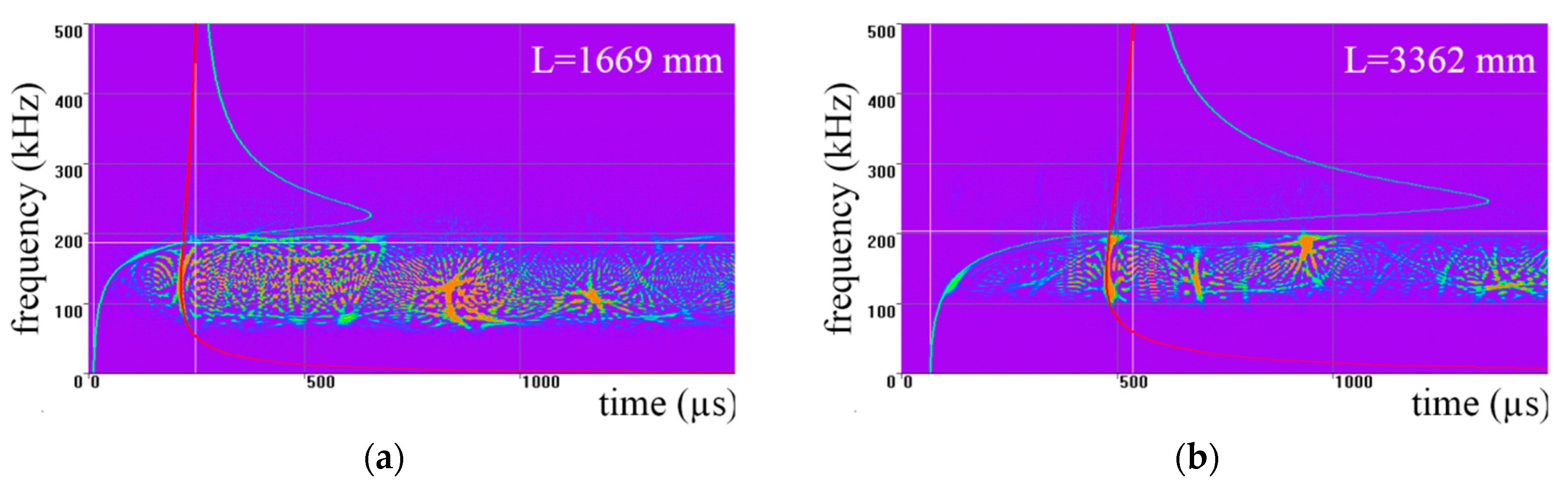
In addition, the spectrograms of the signals on the struts were analyzed, which made it possible to determine the arrival times of different frequency components (Figure 28). It was confirmed that the signals were emitted by impulsive sources and propagated along the walls of the object as Lamb waves. With the help of the spectrogram analysis, the distances between the AE sources and AE sensors were obtained, which coincided with the results of the usual linear location based on the analysis of the arrival times difference [27,28].

At the points on the struts revealed as defective by the AE testing, an additional ultrasonic testing was carried out. On the left strut, 1 crack was found with the size of 20 mm, on the right—1 crack with the size 30 mm.

At present, the question of the SHM-system design for the testing of draglines is under consideration.

4. Conclusions

• Based on our improved AE system, structural AE monitoring scheme is developed as SHM-system. Examples of its successful application are given.
• Oil refinery: Overheating induced the formation of defects at the hydrotreater at the oil refinery plant. The use of SHM-system allowed to extend the lifetime of the hydrotreater by 6 months and to prevent the destruction of the hydrotreater during operation. Cluster analysis method of the AE data was developed and carried out.
• Bridges: As a result of a series of experimental studies, the basic principles have been formulated, which make it possible to improve the efficiency of AE method as applied to the SHM of bridge structures. The solutions for their implementation have been suggested. The acoustic noises arising in monitoring of bridge structures have been analyzed and the causes of noise such as vibrations and friction due to the passing vehicles and wind gusts have been revealed. The multi-stage algorithm of noise filtering has been offered that includes selection by AE parameters.
• Pipelines: Experimental work was carried out on the AE monitoring of the high-temperature process pipeline. The most suitable was the use of the frequency range 150–500 kHz and the threshold in the region of 40–55 dB_AE. It was found that the activity and amplitudes of noise increase significantly when the rate of pipeline temperature change exceeds 1°C/min. It is revealed that the attenuation coefficient essentially increases with the accumulation of sediments in the internal volume of the pipeline. The possibility of detecting melt leakage through flange joints is shown, even if it is invisible under a layer of thermal insulation and is not noticeable.
• Gas adsorbers: In the upper part of the gas adsorber at the refinery, non-permissible defects were found. A decision was made to install a system for SHM for the upper part of the gas adsorber. The main task of the installed monitoring system was to ensure safe operation of the gas adsorber until it can be replaced in a year.
• Support rollers of rotary kiln: The possibility to conduct AE testing of support rollers of rotary kilns in operating mode has been investigated. It was found that in the range above 30 kHz the acoustic noises generally are no more than 32 dB_AE. For full testing of all 3 bearings it is necessary to mount 3 AE sensors on each of 2 bearing enclosures. To perform full AE testing of shaft it is sufficient to provide access to the shaft by removing protective caps and to mount 2 AE sensors: one on the side of thrust bearing and one on the opposite side. The signals with amplitude of about 100 dB_AE, duration of more than 100,000 µs allows us to estimate the needed lubrication intervals. The higher values of AE signal RMS are observed on the shafts of support rollers with long lifetime. While testing the support rollers, the AE sources activity was registered on 2 shafts in the area of fillet. They presumably correspond to active fatigue cracks.
• Dragline excavator: Work was carried out on AE monitoring of boom, column and struts of a walking dragline excavator. To remove noise, the use of a frequency range of 150–500 kHz and a threshold of 50 dB_AE was most appropriate. With these settings, the AE activity acquires a cyclic character synchronized with the excavator operation cycle. By the results of attenuation measuring the recommended distance between the AE sensors is from 4.5 to 9 m. The AE data was collected for 2 days. Six sources of AE have been detected on the left and right struts. When performing ultrasound testing, 2 of them were classified as 20 and 30 mm cracks.