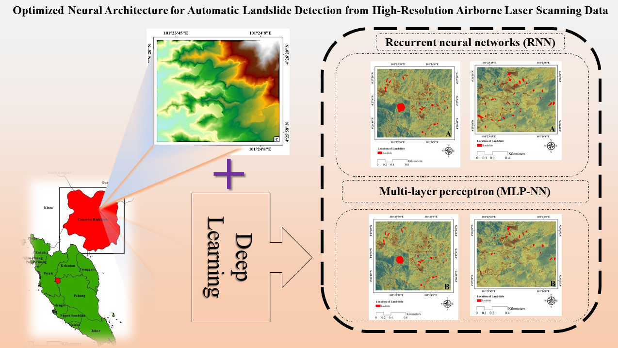
Optimized Neural Architecture for Automatic Landslide Detection from High‐Resolution Airborne Laser Scanning Data


 ,
,
Abstract
:
1. Introduction
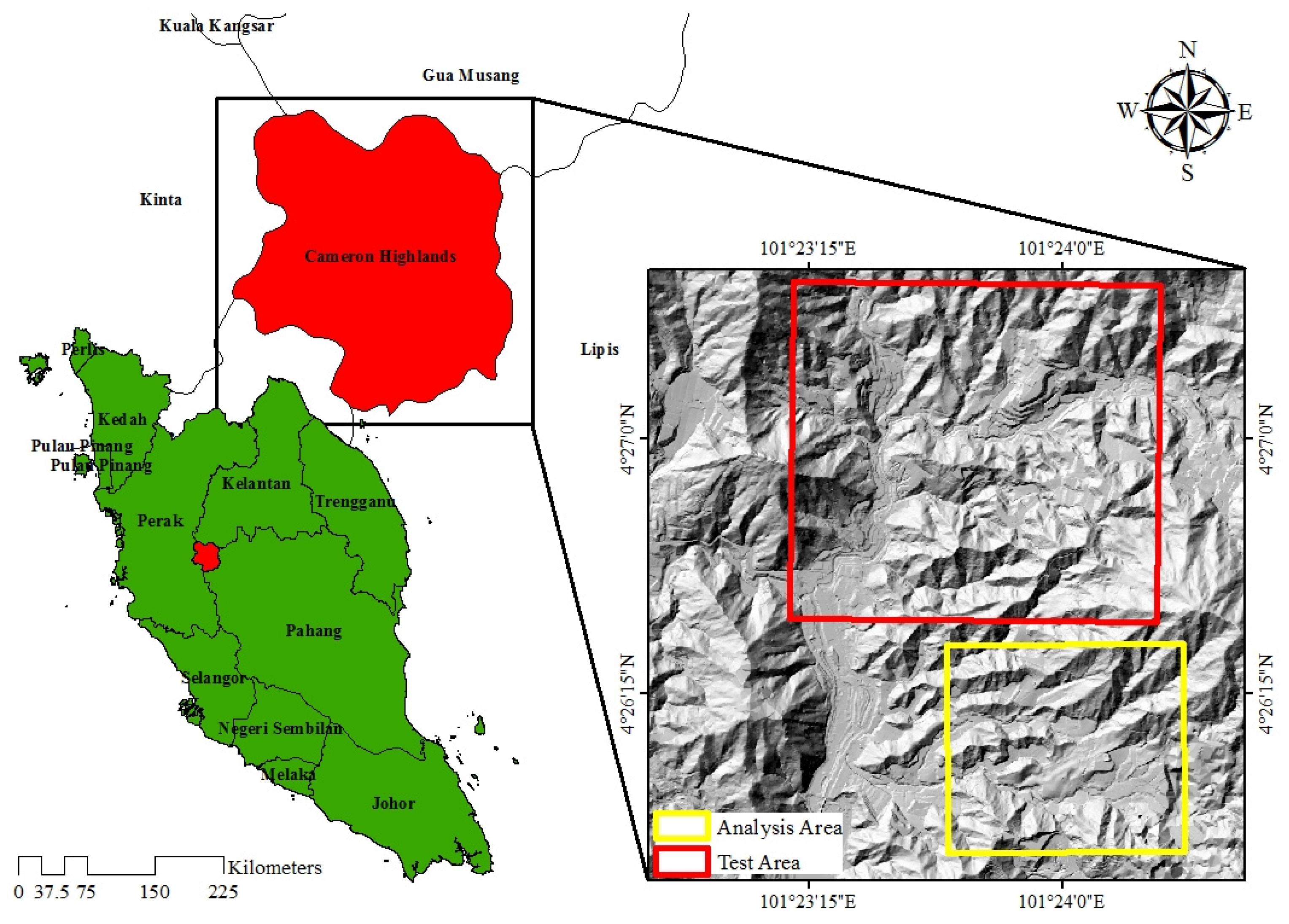
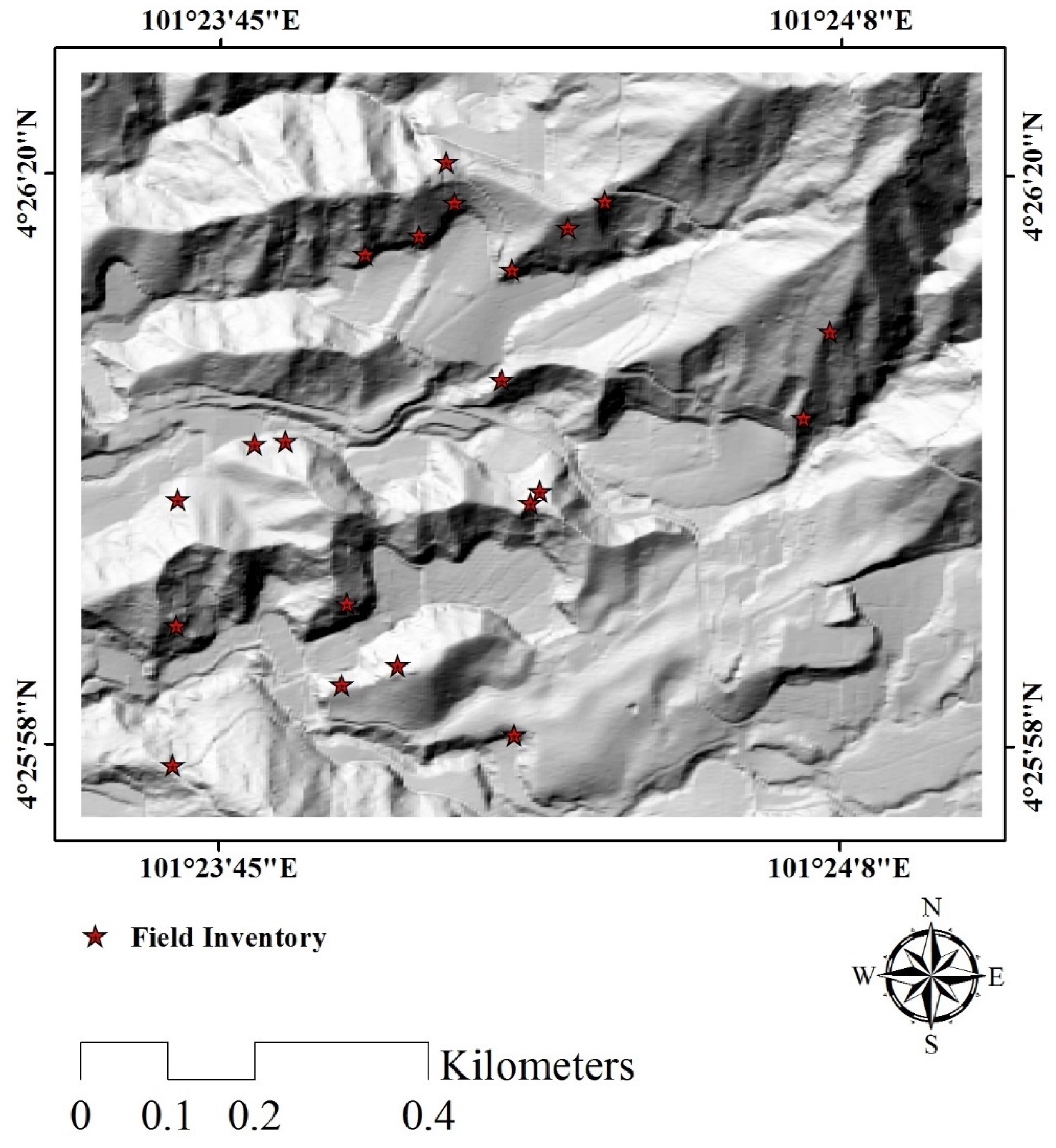
2. Study Area
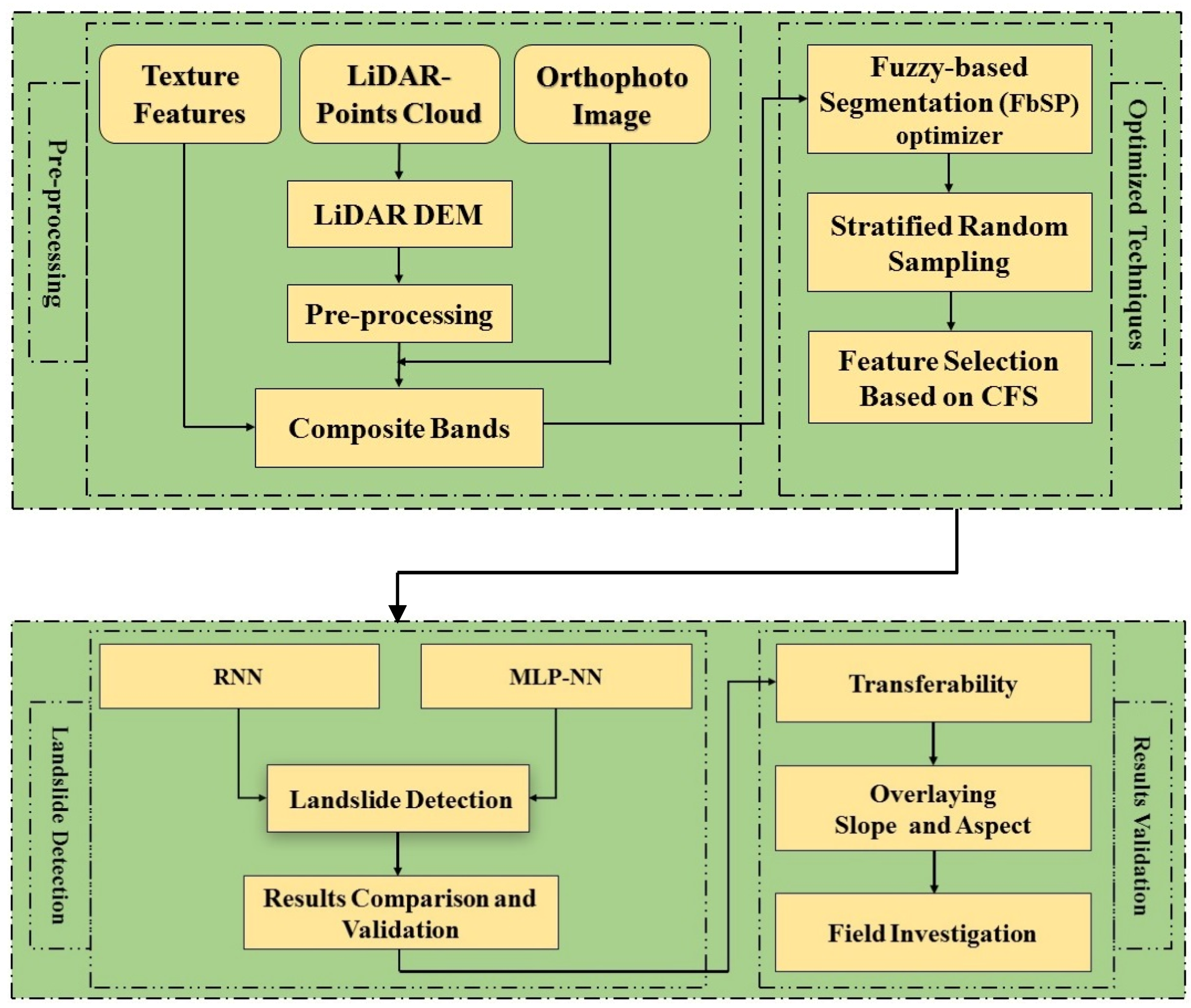
3. Methodology
3.1. Overall Methodology and Pre-Processing
3.2. Landslide Inventory
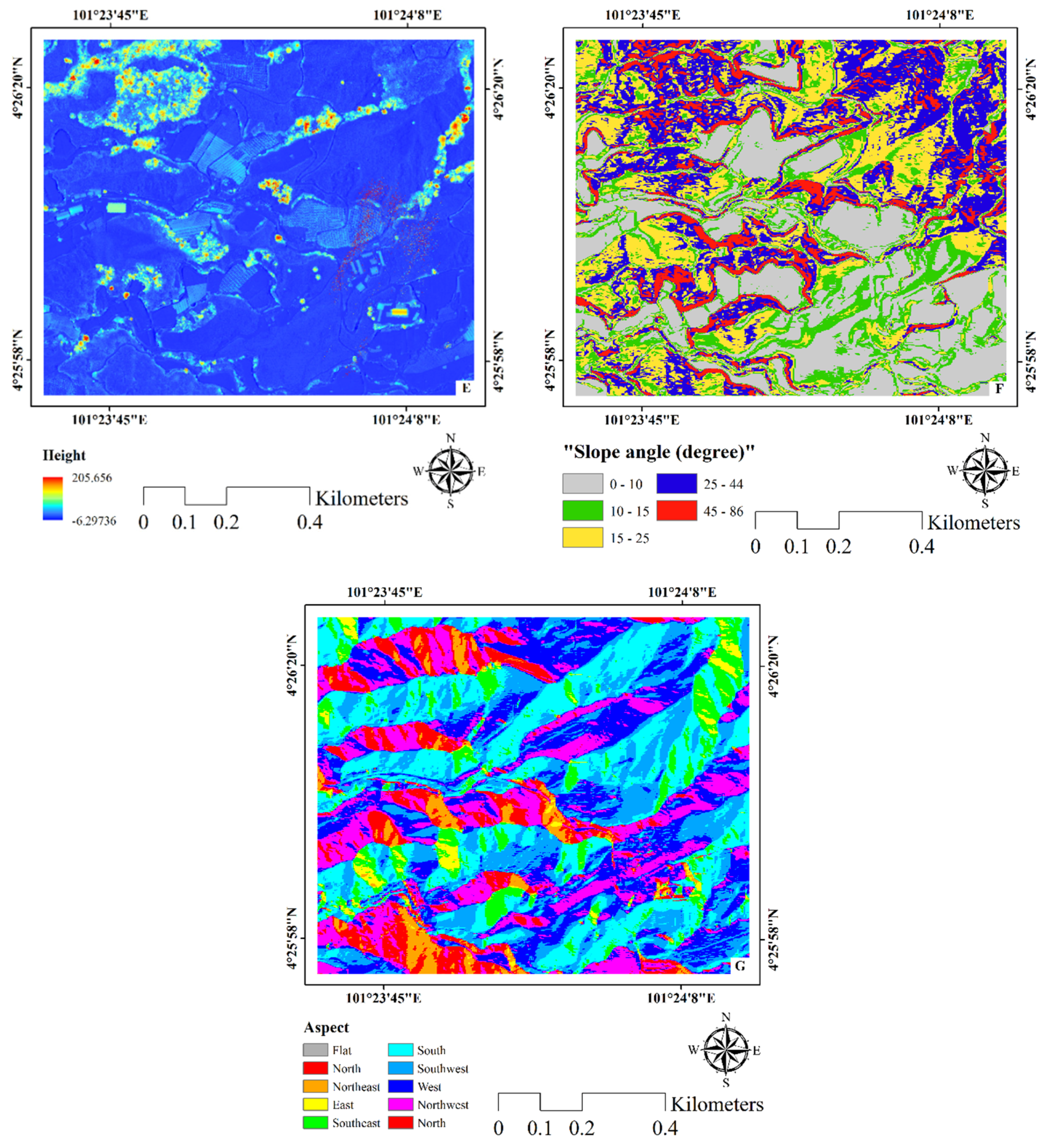
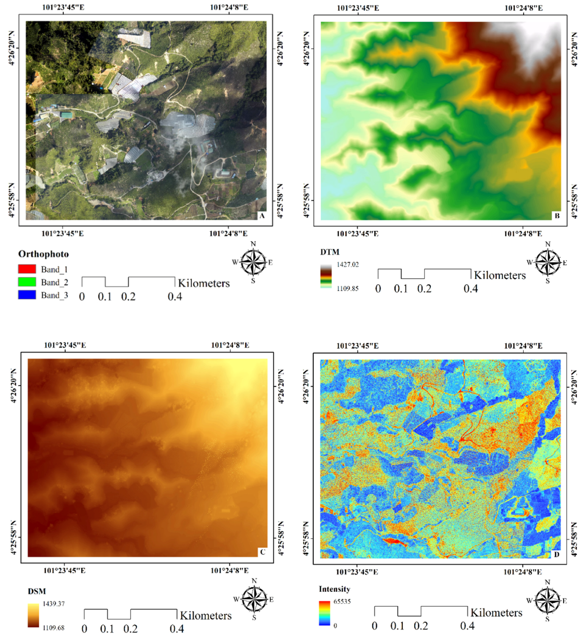
3.3. Data
3.4. Image Segmentation
3.5. Training Sets
3.6. Correlation-Based Feature Selection
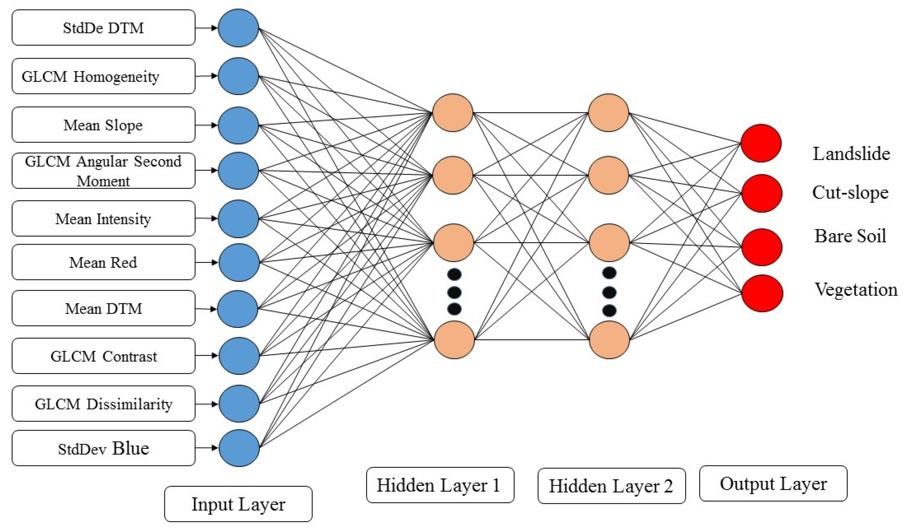
3.7. MLP-NN
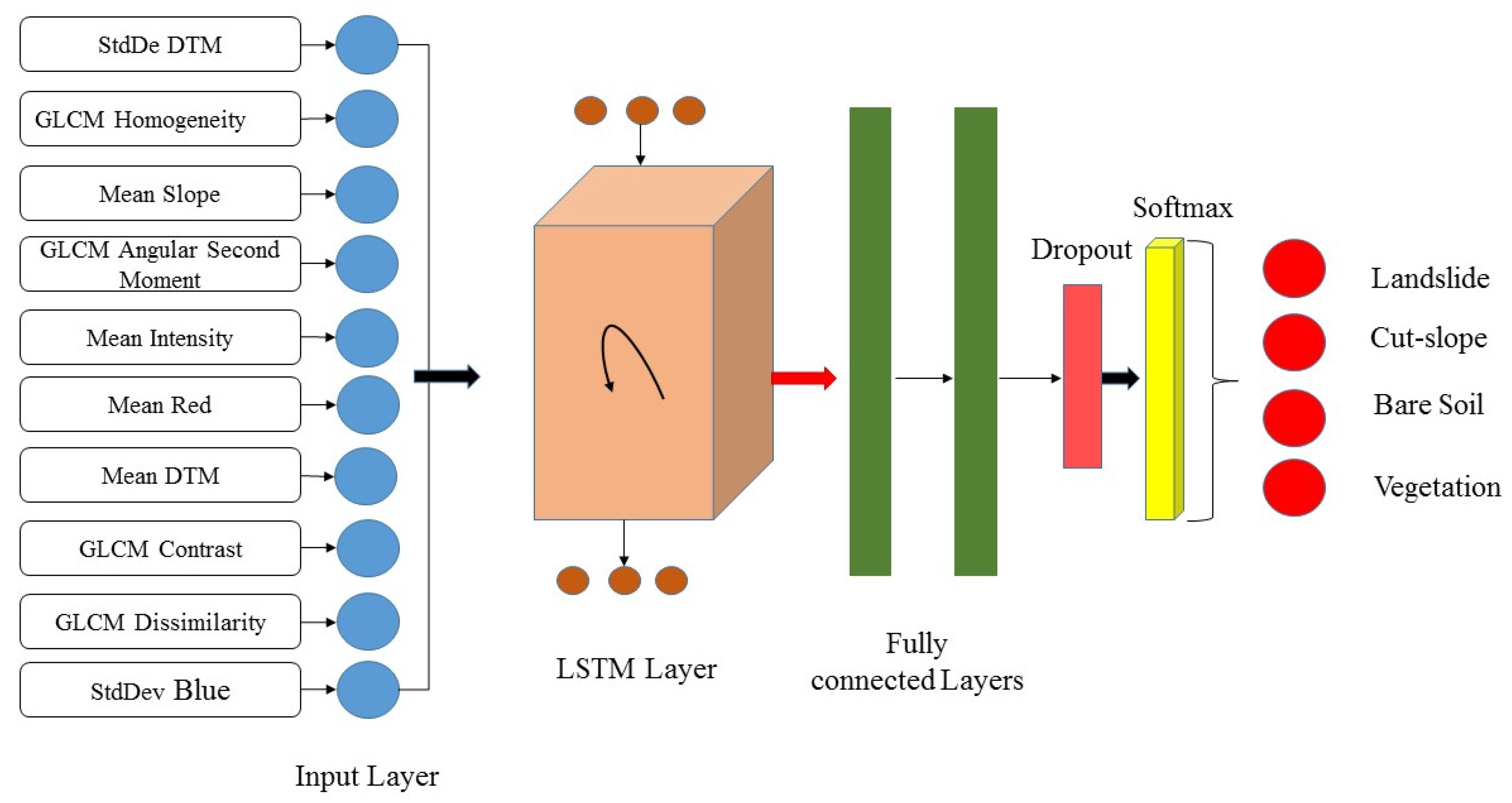
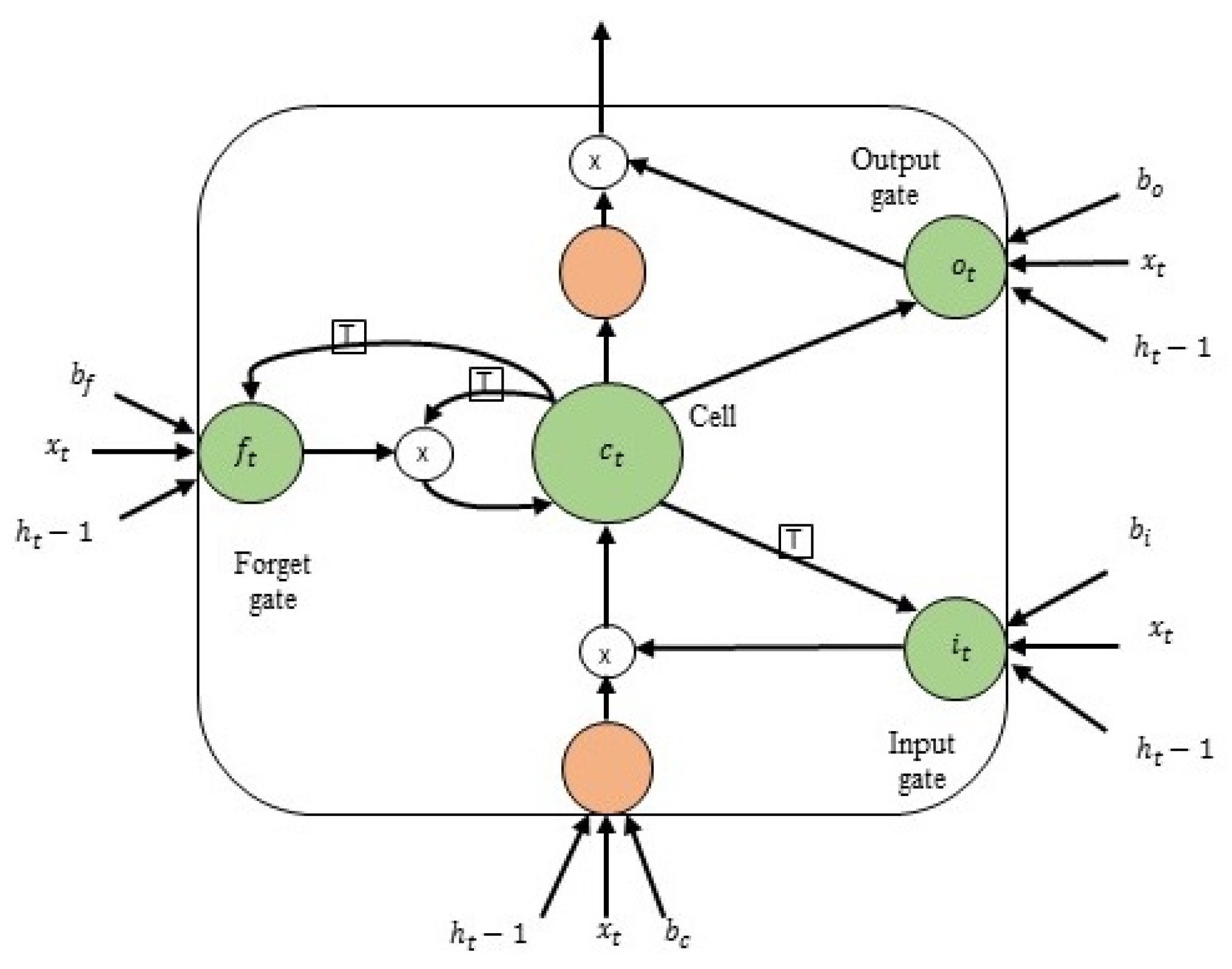
3.8. RNN
3.9. Neural Network Models
3.9.1. MLP-NN
3.9.2. RNN
3.9.3. Optimization of Model Hyper-Parameters
4. Results and Discussion
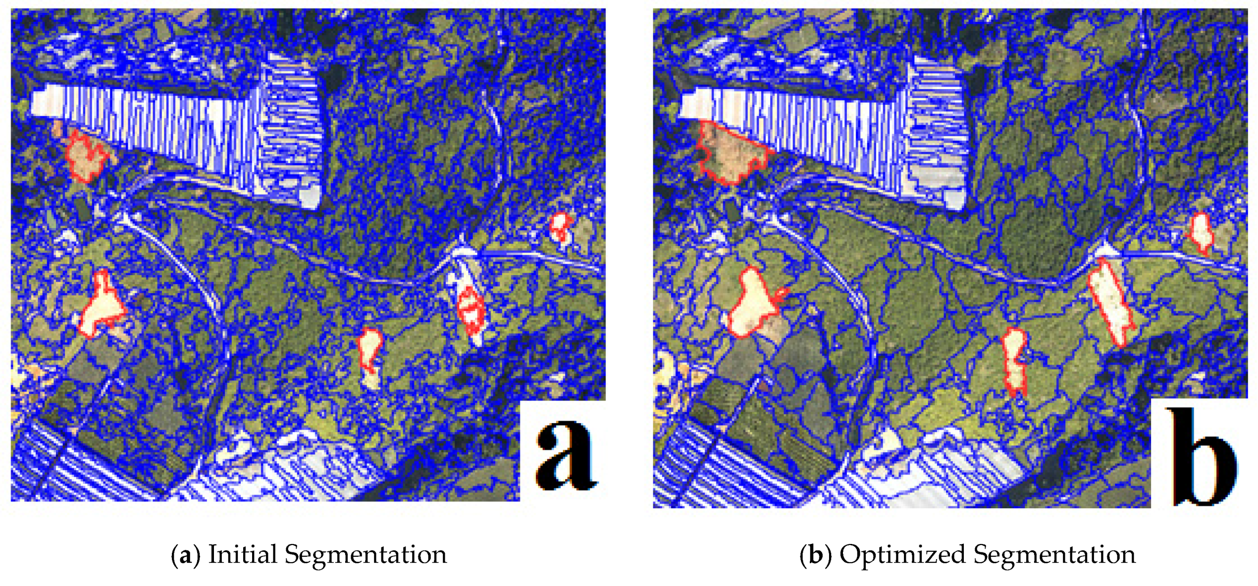
4.1. Supervised Approach for Optimizing Segmentation
4.2. Relevant Feature Subset Based on a CFS Algorithm
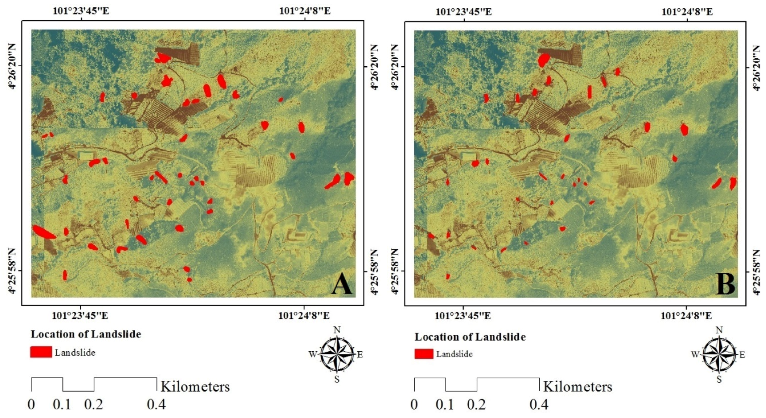
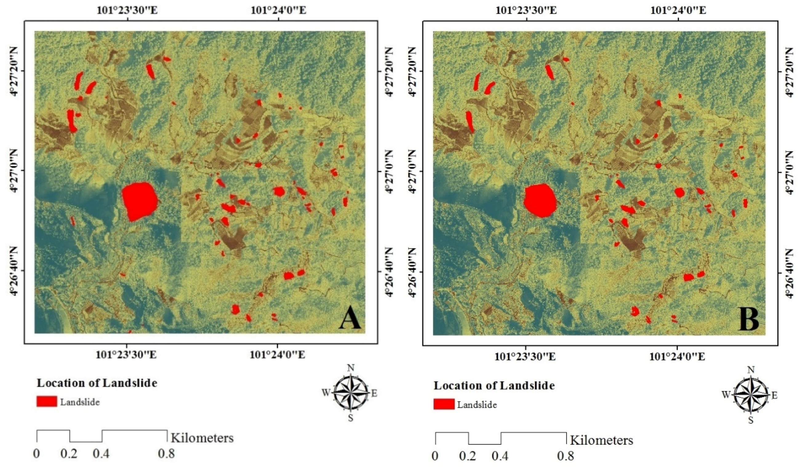
4.3. Results of Landslide Detection
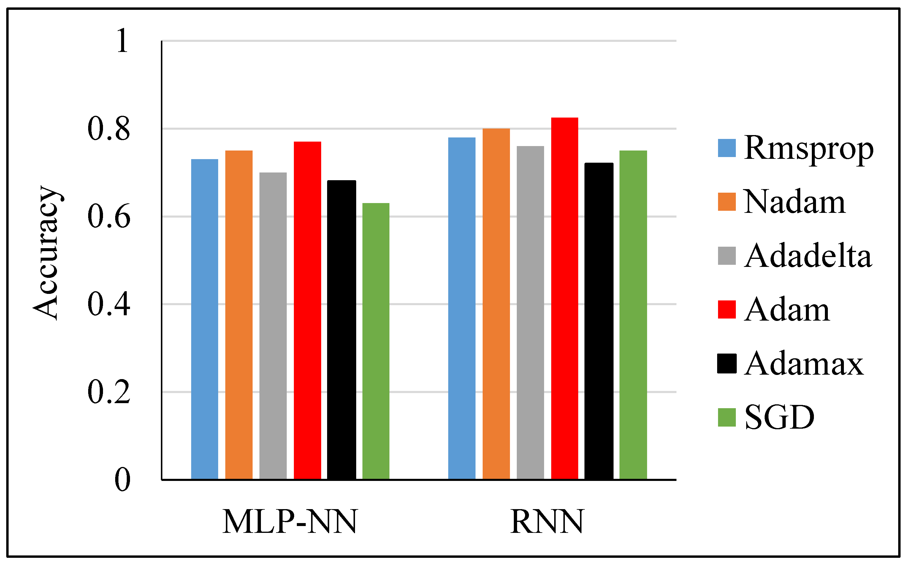
4.4. Performance of the MLP-NN and RNN
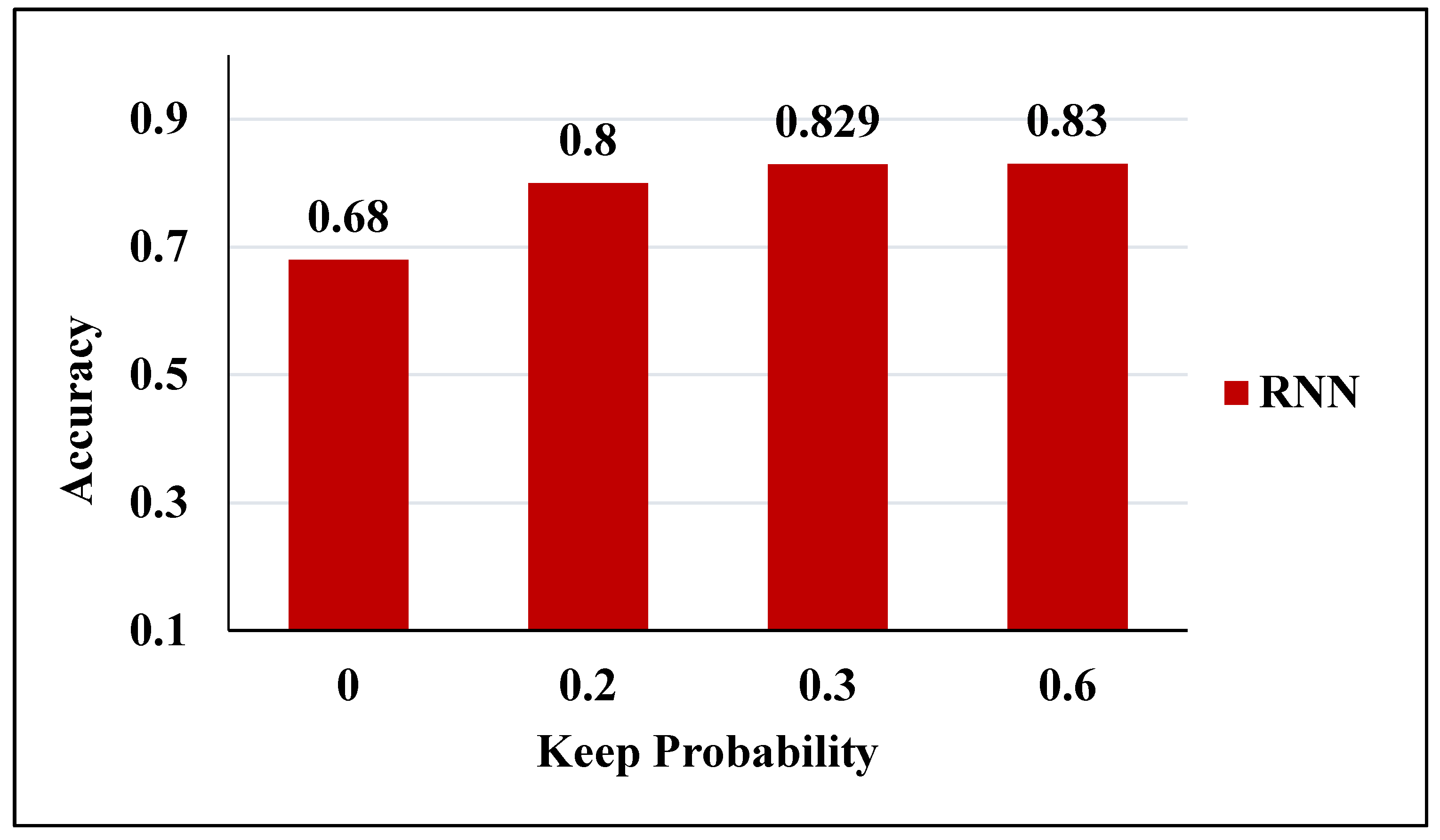
4.5. Sensitivity Analysis
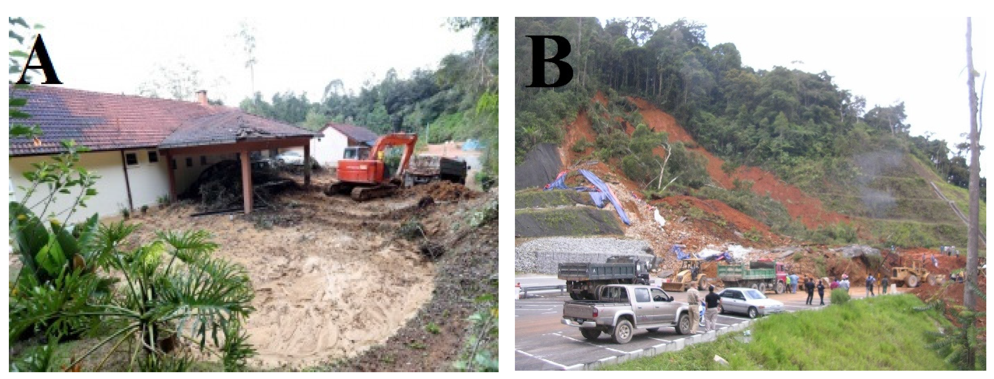
4.6. Field Investigation
5. Conclusion
Author Contributions
Conflicts of Interest
References
- Guzzetti, F.; Mondini, A.C.; Cardinali, M.; Fiorucci, F.; Santangelo, M.; Chang, K.-T. Landslide inventory maps: New tools for an old problem. Earth-Sci. Rev. 2012, 112, 42–66. [Google Scholar] [CrossRef]
- Van Westen, C.J.; Castellanos, E.; Kuriakose, S.L. Spatial data for landslide susceptibility, hazard, and vulnerability assessment: An overview. Eng. Geol. 2008, 102, 112–131. [Google Scholar] [CrossRef]
- Parker, R.N.; Densmore, A.L.; Rosser, N.J.; De Michele, M.; Li, Y.; Huang, R.; Petley, D.N. Mass wasting triggered by the 2008 Wenchuan earthquake is greater than orogenic growth. Nat. Geosci. 2011, 4, 449–452. [Google Scholar] [CrossRef]
- Chen, R.-F.; Lin, C.-W.; Chen, Y.-H.; He, T.-C.; Fei, L.-Y. Detecting and Characterizing Active Thrust Fault and Deep-Seated Landslides in Dense Forest Areas of Southern Taiwan Using Airborne LiDAR DEM. Remote Sens. 2015, 7, 15443–15466. [Google Scholar] [CrossRef]
- Pradhan, B.; Jebur, M.N.; Shafri, H.Z.M.; Tehrany, M.S. Data Fusion Technique Using Wavelet Transform and Taguchi Methods for Automatic Landslide Detection From Airborne Laser Scanning Data and QuickBird Satellite Imagery. IEEE Trans. Geosci. Remote Sens. 2016, 54, 1610–1622. [Google Scholar] [CrossRef]
- McKean, J.; Roering, J. Objective landslide detection and surface morphology mapping using high-resolution airborne laser altimetry. Geomorphology. 2004, 57, 331–351. [Google Scholar] [CrossRef]
- Whitworth, M.; Giles, D.; Murphy, W. Airborne remote sensing for landslide hazard assessment: A case study on the Jurassic escarpment slopes of Worcestershire, UK. Q. J. Eng. Geol. Hydrogeol. 2005, 38, 285–300. [Google Scholar] [CrossRef]
- Blaschke, T. Object based image analysis for remote sensing. ISPRS J. Photogramm. Remote Sens. 2010, 65, 2–16. [Google Scholar] [CrossRef]
- Pradhan, B.; Mezaal, M.R. Optimized Rule Sets for Automatic Landslide Characteristic Detection in a Highly Vegetated Forests. In Laser Scanning Applications in Landslide Assessment; Springer: New York, NY, USA, 2017; pp. 51–68. [Google Scholar]
- Anders, N.S.; Seijmonsbergen, A.C.; Bouten, W. Segmentation optimization and stratified object-based analysis for semi-automated geomorphological mapping. Remote Sens. Environ. 2011, 115, 2976–2985. [Google Scholar] [CrossRef]
- Belgiu, M.; Drǎguţ, L. Comparing supervised and unsupervised multiresolution segmentation approaches for extracting buildings from very high resolution imagery. ISPRS J. Photogramm. Remote Sens. 2014, 96, 67–75. [Google Scholar] [CrossRef] [PubMed]
- Drǎguţ, L.; Tiede, D.; Levick, S.R. ESP: A tool to estimate scale parameter for multiresolution image segmentation of remotely sensed data. Int. J. Geogr. Inf. Sci. 2010, 24, 859–871. [Google Scholar] [CrossRef]
- Zhang, Y.; Maxwell, T.; Tong, H.; Dey, V. Development of a supervised software tool for automated determination of optimal segmentation parameters for ecognition. In Proceedings of the ISPRS TC VII Symposium–100 Years, ISPRS, Vienna, Austria, 5–7 July 2010. [Google Scholar]
- Chen, W.; Li, X.; Wang, Y.; Chen, G.; Liu, S. Forested landslide detection using LiDAR data and the random forest algorithm: A case study of the Three Gorges, China. Remote Sens. Environ. 2014, 152, 291–301. [Google Scholar] [CrossRef]
- Kursa, M.B.; Rudnicki, W.R. Feature selection with the Boruta package. J. Stat. Softw. 2010, 36, 1–13. [Google Scholar] [CrossRef]
- Li, X.; Cheng, X.; Chen, W.; Chen, G.; Liu, S. Identification of forested landslides using LiDar data, object-based image analysis, and machine learning algorithms. Remote Sens. 2015, 7, 9705–9726. [Google Scholar] [CrossRef]
- Stumpf, A.; Kerle, N. Object-oriented mapping of landslides using Random Forests. Remote Sens. Environ. 2011, 115, 2564–2577. [Google Scholar] [CrossRef]
- Borghuis, A.; Chang, K.; Lee, H. Comparison between automated and manual mapping of typhoon-triggered landslides from SPOT-5 imagery. Int. J. Remote Sens. 2007, 28, 1843–1856. [Google Scholar] [CrossRef]
- Danneels, G.; Pirard, E.; Havenith, H.B. Automatic landslide detection from remote sensing images using supervised classification methods. In Geoscience and Remote Sensing Symposium; IEEE: Hoboken, NJ, USA, July 2007; pp. 3014–3017. [Google Scholar]
- Moine, M.; Puissant, A.; Malet, J.-P. Detection of Landslides from Aerial and Satellite Images with a Semi-Automatic Method. Application to the Barcelonnette Basin (Alpes-de-Hautes-Provence, France). February 2009, pp. 63–68. Available online: https://halshs.archives-ouvertes.fr/halshs-00467545/document (accessed on 16 July 2017).
- Pratola, C.; Del Frate, F.; Schiavon, G.; Solimini, D.; Licciardi, G. Characterizing land cover from X-band COSMO-SkyMed images by neural networks. In Proceedings of the Urban Remote Sensing Event (JURSE), Munich, Germany, 11–13 April 2011; pp. 49–52. [Google Scholar]
- Singh, A.; Singh, K.K. Satellite image classification using Genetic Algorithm trained radial basis function neural network, application to the detection of flooded areas. J. Vis. Commun. Image Represent. 2017, 42, 173–182. [Google Scholar] [CrossRef]
- Singh, K.K.; Singh, A. Detection of 2011 Sikkim earthquake-induced landslides using neuro-fuzzy classifier and digital elevation model. Nat. Hazards 2016, 83, 1027–1044. [Google Scholar] [CrossRef]
- Mehrotra, A.; Singh, K.K.; Nigam, M.J.; Pal, K. Detection of tsunami-induced changes using generalized improved fuzzy radial basis function neural network. Nat. Hazards 2015, 77, 367–381. [Google Scholar] [CrossRef]
- Benediktsson, J.A.; Sveinsson, J.R. Feature extraction for multisource data classification with artificial neural networks. Int J. Remote Sens. 1997, 18, 727–740. [Google Scholar] [CrossRef]
- Yuan, H.; Van Der Wiele, C.F.; Khorram, S. An automated artificial neural network system for land use/land cover classification from Landsat TM imagery. Remote Sens. 2009, 1, 243–265. [Google Scholar] [CrossRef]
- Fu, G.; Liu, C.; Zhou, R.; Sun, T.; Zhang, Q. Classification for High Resolution Remote Sensing Imagery Using a Fully Convolutional Network. Remote Sens. 2017, 9, 498. [Google Scholar] [CrossRef]
- Sameen, M.I.; Pradhan, B. Severity Prediction of Traffic Accidents with Recurrent Neural Networks. Appl. Sci. 2017, 7, 476. [Google Scholar] [CrossRef]
- Gorsevski, P.V.; Brown, M.K.; Panter, K.; Onasch, C.M.; Simic, A.; Snyder, J. Landslide detection and susceptibility mapping using LiDAR and an artificial neural network approach: A case study in the Cuyahoga Valley National Park, Ohio. Landslides 2016, 13, 467–484. [Google Scholar] [CrossRef]
- Chang, K.T.; Liu, J.K.; Chang, Y.M.; Kao, C.S. An Accuracy Comparison for the Landslide Inventory with the BPNN and SVM Methods. Gi4DM 2010; Turino, Italy, 2010. Available online: https://www.researchgate.net/profile/Jin_King_Liu/publication/267709454_An_Accuracy_Comparison_for_the_Landslide_Inventory_with_the_BPNN_and_SVM_Methods/links/5511773f0cf29a3bb71de12c.pdf (accessed on 20 March 2017).
- Robert, H.N. Neurocomputing; Addison-Wesley Pub. Co.: Boston, CA, USA, 1990; pp. 21–42. [Google Scholar]
- Zurada, J.M. Introduction to Artificial Neural Systems; West Pub. Co.: Eagan, MN, USA, 1992; pp. 163–248. [Google Scholar]
- Chang, K.T.; Liu, J.K. Landslide features interpreted by neural network method using a high-resolution satellite image and digital topographic data. In Proceedings of the XXth ISPRS Congress, Istanbul, Turkey, 12–23 July 2004. [Google Scholar]
- Chen, H.; Zeng, Z.; Tang, H. Landslide deformation prediction based on recurrent neural network. Neural Process. Lett. 2015, 41, 169–178. [Google Scholar] [CrossRef]
- Ma, H.-R.; Cheng, X.; Chen, L.; Zhang, H.; Xiong, H. Automatic identification of shallow landslides based on Worldview2 remote sensing images. J. Appl. Remote Sens. 2016, 10, 016008. [Google Scholar] [CrossRef]
- Hall, M.A. Correlation-based Feature Selection for Machine Learning. Doctoral dissertation, The University of Waikato, Hamilton, New Zealand, April 1999. [Google Scholar]
- Miner, A.; Flentje, P.; Mazengarb, C.; Windle, D. Landslide Recognition Using LiDAR Derived Digital Elevation Classifiers-Lessons Learnt from Selected Australian Examples. Available online: http://ro.uow.edu.au/cgi/viewcontent.cgi?article=1590&context=engpapers (accessed on 10 June 2017).
- Martha, T.R.; Kerle, N.; van Westen, C.J.; Jetten, V.; Kumar, K.V. Segment optimization and data-driven thresholding for knowledge-based landslide detection by object-based image analysis. IEEE Trans. Geosci. Remote Sens. 2011, 49, 4928–4943. [Google Scholar] [CrossRef]
- Pradhan, B.; Lee, S. Regional landslide susceptibility analysis using back-propagation neural network classifier at Cameron Highland, Malaysia. Landslides 2010, 7, 13–30. [Google Scholar] [CrossRef]
- Olaya, V. Basic land-surface parameters. Dev. Soil Sci. 2009, 33, 141–169. [Google Scholar]
- Barbarella, M.; Fiani, M.; Lugli, A. Application of LiDAR-derived DEM for detection of mass movements on a landslide. Int. Arch. Photogramm. Remote Sens. Spat. Inf. Sci. 2013, 1, 89–98. [Google Scholar] [CrossRef]
- Duro, D.C.; Franklin, S.E.; Dubé, M.G. Multi-scale object-based image analysis and feature selection of multi-sensor earth observation imagery using random forests. Int. J. Remote Sens. 2012, 33, 4502–4526. [Google Scholar] [CrossRef]
- Kohavi, R.; John, G.H. Wrappers for feature subset selection. Artif. Intell. 1997, 97, 273–324. [Google Scholar] [CrossRef]
- Mokhtarzade, M.; Zoej, M.V. Road detection from high-resolution satellite images using artificial neural networks. Int. J. Appl. Earth Obs. Geoinf. 2007, 9, 32–40. [Google Scholar] [CrossRef]
- Gardner, M.W.; Dorling, S.R. Artificial neural networks (the multilayer perceptron)—A review of applications in the atmospheric sciences. Atmos. Environ. 1998, 32, 2627–2636. [Google Scholar] [CrossRef]
- Baczyński, D.; Parol, M. Influence of artificial neural network structure on quality of short-term electric energy consumption forecast. IEE Proc.-Gener., Transm. Distrib. 2004, 151, 241–245. [Google Scholar] [CrossRef]
- Mia, M.M.A.; Biswas, S.K.; Urmi, M.C.; Siddique, A. An algorithm for training multilayer perceptron (MLP) for Image reconstruction using neural network without overfitting. Int. J. Sci. Techno. Res. 2015, 4, 271–275. [Google Scholar]
- Yang, G.Y.C. Geological Mapping from Multi-Source Data Using Neural Networks; Geomatics Engineering, University of Calgary: Calgary, AB, Canada, 1995. [Google Scholar]
- Hochreiter, S.; Schmidhuber, J. Long short-term memory. Neural Comput. 1997, 9, 1735–1780. [Google Scholar] [CrossRef] [PubMed]
- Donahue, J.; Anne Hendricks, L.; Guadarrama, S.; Rohrbach, M.; Venugopalan, S.; Saenko, K.; Darrell, T. Long-Term Recurrent Convolutional Networks for Visual Recognition and Description. In Proceedings of the IEEE conference on computer vision and pattern recognition, Boston, MA, USA, 7–12 June 2015; pp. 2625–2634. [Google Scholar]
- Pedregosa, F.; Varoquaux, G.; Gramfort, A.; Michel, V.; Thirion, B.; Grisel, O.; Vanderplas, J. Scikit-learn: Machine learning in Python. J. Mach. Learn. Res. 2011, 12, 2825–2830. [Google Scholar]
- Sameen, M.I.; Pradhan, B.; Shafri, H.Z.; Mezaal, M.R.; bin Hamid, H. Integration of Ant Colony Optimization and Object-Based Analysis for LiDAR Data Classification. IEEE J. Sel. Top. Appl. Earth Obs. Remote Sens. 2017, 10, 2055–2066. [Google Scholar] [CrossRef]
- Bartels, M.; Wei, H. Threshold-free object and ground point separation in LIDAR data. Pattern Recognit. Lett. 2010, 31, 1089–1099. [Google Scholar] [CrossRef]
- Rau, J.Y.; Jhan, J.P.; Rau, R.J. Semiautomatic object-oriented landslide recognition scheme from multisensor optical imagery and DEM. IEEE Trans. Geosci. Remote Sens. 2011, 52, 1336–1349. [Google Scholar] [CrossRef]


| Class Name | Number of the Object for Each Class |
|---|---|
| Landslide | 52 |
| Cut slope | 67 |
| Bare soil | 80 |
| Vegetation | 150 |
| Optimized Parameter | Suitable Value | Description |
|---|---|---|
| Minibatch size | 126 (RNN) 64 (MLP-NN) | Number of training cases over which the Adam update is computed. |
| Loss function | categorical cross-entropy | The objective function or optimization score function is also called as multiclass legless, which is appropriate for categorical targets. |
| Optimizer | Adam | Adaptive moment estimation |
| dropout rates | 0.6 | Dropping out units (hidden and visible) |
| Initial Parameters | Optimal Parameters | |||||
|---|---|---|---|---|---|---|
| Number | Scale | Shape | Compactness | Scale | Shape | Compactness |
| 1 | 50 | 0.1 | 0.1 | 75.52 | 0.4 | 0.5 |
| 2 | 80 | 0.1 | 0.1 | 100 | 0.45 | 0.74 |
| Feature | Iteration | Rank |
|---|---|---|
| StdDe DTM | 20 | 1 |
| GLCM homogeneity | 18 | 2 |
| Mean slope | 20 | 3 |
| GLCM angular second moment | 20 | 4 |
| Mean intensity | 17 | 5 |
| Mean red | 20 | 6 |
| Mean DTM | 20 | 7 |
| GLCM contrast | 18 | 8 |
| GLCM dissimilarity | 15 | 9 |
| StdDev blue | 20 | 10 |
| Neural Network Model | Analysis Area | Test Area |
|---|---|---|
| RNN model | 83.33% | 81.11% |
| MLP-NN model | 78.38% | 74.56% |
© 2017 by the authors. Licensee MDPI, Basel, Switzerland. This article is an open access article distributed under the terms and conditions of the Creative Commons Attribution (CC BY) license (http://creativecommons.org/licenses/by/4.0/).
Share and Cite
Mezaal, M.R.; Pradhan, B.; Sameen, M.I.; Mohd Shafri, H.Z.; Yusoff, Z.M. Optimized Neural Architecture for Automatic Landslide Detection from High‐Resolution Airborne Laser Scanning Data. Appl. Sci. 2017, 7, 730. https://doi.org/10.3390/app7070730
Mezaal MR, Pradhan B, Sameen MI, Mohd Shafri HZ, Yusoff ZM. Optimized Neural Architecture for Automatic Landslide Detection from High‐Resolution Airborne Laser Scanning Data. Applied Sciences. 2017; 7(7):730. https://doi.org/10.3390/app7070730
Chicago/Turabian StyleMezaal, Mustafa Ridha, Biswajeet Pradhan, Maher Ibrahim Sameen, Helmi Zulhaidi Mohd Shafri, and Zainuddin Md Yusoff. 2017. "Optimized Neural Architecture for Automatic Landslide Detection from High‐Resolution Airborne Laser Scanning Data" Applied Sciences 7, no. 7: 730. https://doi.org/10.3390/app7070730