


Abstract
This study develops a data-driven Gaussian process-based model predictive control (GP-MPC) method for an interacting nonlinear gas–liquid system. Three independent Gaussian process models with Matérn 5/2 kernels are trained to predict the gas flowrate, gas-side pressure and liquid-side pressure from the states, two equivalent pressure commands and pressure-command increments. The mean predictions from the three GP models are recursively propagated within the MPC formulation, which accounts for flow tracking, pressure imbalance, control variation, terminal tracking error, convergence, input constraints and online flowrate bias correction. The GP models and MPC optimization are executed on a Raspberry Pi 3, while a physics-based gas–liquid plant model is implemented in MATLAB R2026a/Simulink-Simscape and connected through TCP/IP in a hardware-in-the-loop configuration with a sampling period of 0.1 s. All three GP models achieved validation R2 scores above 0.99998, while the gas-flow model achieved an RMSE of 0.2447 L/min over a 50-step recursive prediction horizon. At references of 8.3, 16.6 and 25 L/min, settling times ranged from 2.5 to 6.8 s, with steady-state errors below 0.121% and overshoots below 0.285%. Under continuous bidirectional reference changes, the controller achieved an RMSE of 0.654 L/min and an MAE of 0.091 L/min, with settling times between 1.9 and 3.7 s.
1. Introduction
Gas–liquid transport in membrane-based contacting systems occurs across a defined interface between the two phases, allowing gas–liquid mass transfer without direct dispersion of one phase into the other. Maintaining an appropriate pressure difference across this interface is an important operating requirement because the pressure balance determines the location and stability of the gas–liquid interface within a porous membrane. For hydrophobic membranes, excessive liquid-side pressure relative to the gas side can exceed the breakthrough pressure and promote liquid penetration or membrane wetting [1]. Polytetrafluoroethylene (PTFE) is widely used as a membrane material because of its intrinsic hydrophobicity and high chemical stability, while its porous structure and membrane geometry also influence mass-transfer resistance and gas-transfer performance [2,3]. These coupled transport and pressure-balancing requirements create a control problem in which gas-flow regulation must be coordinated with the pressures on both sides of the interface while respecting operating constraints.
Model-based nonlinear control methods have been investigated for systems involving uncertain and time-varying dynamics. Phan et al. developed an adaptive sliding-mode controller for a blower-based breathing simulator with unknown and time-varying airway resistance and compliance [4]. Truong et al. subsequently combined an identified second-order dynamic model, a disturbance observer and sliding-mode control to improve tracking performance in a ventilation blower-based system under external disturbances [5]. In a wider scope of applications, Le et al. developed a discrete-time model-reference adaptive sliding-mode controller to cope with model uncertainties and disturbances [6]. These studies show how adaptive control and sliding-mode control may be used to increase robustness to parameter uncertainties and disturbances. However, their approach has been centered on tracking and disturbance rejection of particular plants. Conversely, the gas–liquid system considered here involves the simultaneous control of two pressure setpoints, prediction of several coupled process variables, and satisfaction of both input and differential pressure constraints. These requirements are in support of an optimization-based control approach that can handle the multivariable interactions and constraints. Model predictive control (MPC) is ideal for such applications because it predicts future system behavior, optimizes control moves over a finite horizon, and considers the effects of multivariable interactions and constraints. Grancharova et al. developed an explicit MPC strategy for a two-input two-output laboratory gas–liquid separation plant, in which the optimal control law was approximated offline through orthogonal search-tree partitioning to reduce online computation [7]. For the same class of plant, Likar and Kocijan exploited the different bandwidths of the level and pressure control loops to formulate a single-input single-output pressure control problem and implemented predictive control using a Gaussian process (GP) model [8]. Pedersen et al. subsequently applied nonlinear MPC to underbalanced drilling, where pressure and flow variables must be coordinated while satisfying process-dependent operating requirements [9]. These studies demonstrate the suitability of predictive control for interacting fluid systems and exhibit that controller performance depends strongly on the accuracy and computational tractability of the prediction model.
Constructing a sufficiently accurate first-principles model for a nonlinear gas–liquid system can require detailed descriptions of fluid properties, pressure losses, wall and interfacial interactions, and flow-regime-dependent closure relations [10,11]. Inaccurate closure relations and model simplifications can consequently degrade multi-step predictions and closed-loop control performance. Data-driven system identification provides an alternative by learning nonlinear dynamic relationships directly from representative input–output measurement [12]. Among the available learning methods, GP regression provides a flexible nonparametric framework for learning nonlinear mappings while producing both a predictive mean and a variance that represents model confidence [13,14]. Kocijan et al. established the use of GP models for nonlinear dynamic-system identification and showed that dynamic transitions can be learned from lagged measurements and manipulated inputs without specifying an explicit analytical process model [13]. GP models were subsequently incorporated into predictive control, where recursive predictions were used to optimize future control actions [15]. These properties make GP regression particularly attractive for interaction systems in which the dominant nonlinear relationships can be observed from data but are difficult to derive accurately from physical principles. The integration of GP models with MPC has since developed in several directions. Hewing et al. used the nominal model with GP-learned residual dynamics and developed the idea of a cautious MPC controller that considers predicted uncertainty to formulate the chance constraints [16]. Bradford et al. put forward a data-driven stochastic MPC strategy where the GP samples are generated offline in order to compute constraint back-offs, thus alleviating the online computational burden of dealing with uncertainty [17]. In order to safely explore, Koller et al. included statistically reliable GP confidence intervals within a learning-based MPC architecture [18]. For model mismatch problems, Maiworm et al. came up with an online learning-based MPC approach with evolving GP models that includes criteria for recursive satisfaction of constraints and input-to-state stability [19]. Overall, learning-based MPC research has concentrated on the development of prediction models, the management of constraints, online adaptation, and control reliability versus learning efficiency [20]. Practical implementation has also been investigated by recent research. Learning-based GP-MPC was implemented in embedded hardware for mobile robots [21]. On the other hand, L4acados is a new interface to integrate learning-based residual models such as GPs in real-time nonlinear optimal-control solvers [22].
Nevertheless, GP-MPC algorithms remain computationally demanding because online optimization may require repeated evaluation of GP predictions and their associated quantities [23]. Challenges include scalable GP inference, efficient multi-step prediction, uncertainty handling, online adaptation, and reliable constraint treatment [24,25], particularly when the controller is executed with a short sampling period on computationally limited hardware. Representative embedded GP-MPC studies have primarily focused on robotic and autonomous platforms, such as miniature race cars [26] and unmanned quadrotors [27], while recent frameworks such as L4acados facilitate the integration of learning-based models into real-time nonlinear optimal-control solvers [22]. In the gas–liquid application of Likar and Kocijan [8], GP-based predictive control was formulated for a single pressure output and a single manipulated input. In contrast, the present study considers a multivariable gas–liquid system with three predicted process variables, gas flowrate, gas-side pressure, and liquid-side pressure, and two coordinated equivalent pressure commands. The complete GP posterior-mean inference and MPC optimization procedure is executed directly on a Raspberry Pi 3 within a TCP/IP-based HIL configuration operating at a 0.1 s sampling period. Thus, the implementation-oriented distinction of the present study lies in combining multivariable GP-based prediction, coordinated two-input MPC, and low-cost embedded execution for an interacting gas–liquid process.
This study addresses this implementation-oriented gap by developing a data-driven GP-MPC framework for an interacting nonlinear gas–liquid system. The system state consists of the gas flowrate, the gas-side pressure and the liquid-side pressure, while the manipulated variables include the equivalent gas- and liquid-side pressure commands. Predictions for the gas flowrate, gas-side pressure, and liquid-side pressure for the next sampling time are obtained by training three separate GP models. Each model uses a regression input vector comprising the current gas flowrate, gas-side pressure, liquid-side pressure, the two applied pressure commands, and their respective increments, thereby capturing both the current operating condition and the effects of changes in the pressure commands. GP predictive means are propagated recursively during the MPC prediction horizon for computation of coordinated pressure commands for the gas and liquid sides. The optimization objective minimizes gas-flow tracking errors, pressure balance errors, changes in control effort, terminal tracking accuracy, and reference convergence. At the same time, both the pressure command and its increment values are subject to hard limits, while the flowrate bias correction procedure is used to reduce the influence of local GP model errors on the process. In particular, since the designed controller is based on the GP posterior mean as the nominal model of the system transition dynamics, this approach is clearly differentiated from the stochastic GP-MPC where the predictive variance is propagated to guarantee the probabilistic constraints.
With this setup, the GP models and the MPC optimizations are performed on the Raspberry Pi 3 while the nonlinear gas–liquid process is modeled using MATLAB/Simulink-Simscape. The two systems exchange data on states, control input, reference input and optimized control command using TCP/IP communication protocol, thus forming a HIL testing facility with a sampling period of 0.1 s. With this setup, it is possible to test the suggested control algorithm on the physical hardware using a simulated plant; hence, the results obtained constitute a hardware-in-the-loop verification process but not a real experiment performed on the physical gas–liquid system. The model’s accuracy is checked using both one-step-ahead validation and recursive multi-step prediction based on an independent time-ordered test dataset. The performance of the closed-loop system is later investigated at fixed gas flow references and with continuous two-way step changes, taking into consideration tracking error, transient response, and pressure difference.
The principal contributions of this study are summarized as follows:
- A fully data-driven dynamic model comprising three independent GP predictors is developed for the simultaneous prediction of gas flowrate, gas-side pressure and liquid-side pressure. The regression structure combines measured states; two applied pressure commands and pressure increments and its predictive capability are evaluated using both one-step and recursive multi-step tests.
- A multivariable GP-MPC structure is formulated to regulate gas flow through coordinated gas-side and liquid-side pressure commands. The proposed controller recursively propagates GP predictive means, considers input-magnitude and input-rate bounds, regulates the pressure difference between the gas and liquid sides and incorporates online flowrate bias correction.
- The complete GP inference and MPC optimization procedure is deployed on a Raspberry Pi 3 and evaluated in a TCP/IP-based HIL configuration with a sampling period of 0.1 s. Fixed-reference and stepwise-reference scenarios are used to assess tracking accuracy, transient performance, pressure imbalance, and embedded computational feasibility. The 0.1 s value denotes the HIL sampling interval, while computational execution time is evaluated separately from the recorded GP-MPC optimization timing.
2. Materials and Methods
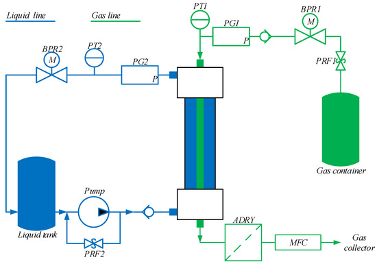
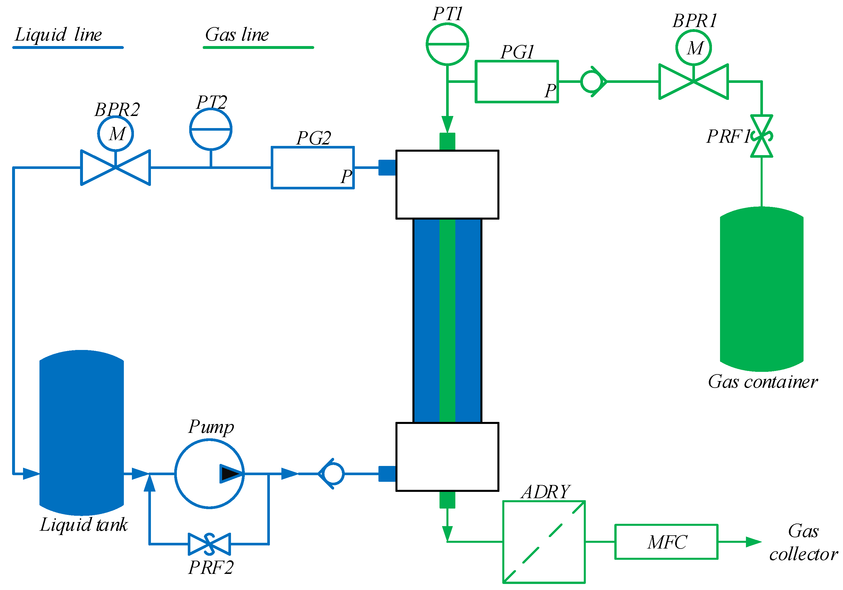
The dual-phase fluidic system consists of a gas flow channel enclosed within a polytetrafluoroethylene (PTFE) tube (Quickun, Ningbo, Zhejiang, China), which is immersed in a surrounding liquid medium. The gas is supplied from a pressurized gas container and regulated by a motorized back-pressure regulator (BPR1) manufactured by Tianjin Tianfei High-Tech Valve Co., Ltd., Tianjin, China. The gas pressure is measured by a pressure transmitter (PT1) from MEASUREMAN, Fuzhou, Jiangxi, China, and a pressure gauge (PG1) from SCTSNSR, Wenzhou, Zhejiang, China. A check valve is installed to ensure unidirectional gas flow toward the membrane module. After entering the PTFE tube, the gas flows through the membrane module and exits toward the downstream line, where it passes through an air dryer (ADRY) from SMC Corporation, Tokyo, Japan and a mass flow controller (MFC) from Alicat Scientific, Tucson, Arizona, USA for flowrate regulation and measurement. On the liquid side, water is drawn from a water tank by a pump and delivered to the outer side of the PTFE tube through a check valve. The liquid pressure is monitored by a pressure transmitter (PT2) from the same manufacturer as PT1 and a pressure gauge (PG2) supplied by the same manufacturer as PG1. The liquid flow and pressure are regulated by a motorized back-pressure regulator (BPR2) provided by the same manufacturer as BPR1.
Let qg,k, pg,k and pl,k denote the gas flowrate, gas-side pressure and liquid-side pressure at time step k, respectively. In the reduced-order HIL model, the manipulated input vector is defined as
where ug,k and ul,k are the equivalent absolute-pressure commands applied to the gas-side and liquid-side controlled pressure sources, respectively. They do not represent motor voltage or valve-opening ratio in the present HIL implementation. The motor and actuator dynamics of the physical back-pressure regulators are omitted from the reduced-order plant model; therefore, no calibration relationship between BPR voltage or valve opening and the equivalent pressure commands is employed in this study. The primary control objectives are (i) to regulate the gas flowrate to the desired reference and (ii) to regulate the pressure difference between the gas and liquid sides.
The pressure difference Δp across the tube is defined as
where pg,k and pl,k denote the gas-side and liquid-side absolute pressures, respectively, and are expressed in bar(a). The differential pressure is expressed in bar. This pressure difference plays a dominant role in governing gas transport through the PTFE interface.
Δpk ≜ pg,k − pl,k,
The dynamics of the dual-phase fluidic system are characterized by the complex interaction between the gas pressure, liquid pressure and effluent mass flowrate. The dual-phase fluidic system is modeled within a discrete-time state-space framework where state vector transitions are governed by an unknown nonlinear mapping to be identified. The state vector is defined as
and the system dynamics are described by
where xk+1 ∈ ℝ3 is the state at the subsequent time step, f(∙) is the unknown nonlinear transition function and represents the additive Gaussian white noise, with σn as the measurement noise standard deviation.
xk+1 = f(xk,uk) + ϵk,
As the mass flowrate qg is a measureable process variable depending on the internal pressure of the gas and the dynamics of the mass flow controller, it is considered an endogenous state variable and not an exogenous control input. Due to the strong coupling between gas and liquid dynamics and the high sensitivity of liquid pressure to changes in the applied pressure commands, the system exhibits fast transient behavior that cannot be captured solely by the instantaneous input values. In particular, rapid pressure variations can occur even for small changes in the equivalent pressure commands. To represent this transient input effect, the regression model is augmented with pressure-command increments. The input increment is defined as
Δuk ≜ uk − uk−1.
Accordingly, the regression vector is constructed as
and the system dynamics (4) can be equivalently written as
xk+1 = f(zk) + ϵk.
The nonlinear mapping f(⋅) defines a transformation f: ℝ7 → ℝ3. In practice, each component of the state transition is modeled independently using a scalar Gaussian process:
where each mapping fs: ℝ7 → ℝ represents the transition function of the s-th state component.
fs(z) ~ (0,k(z,z′)), s = 1, 2, 3,
A Matérn 5/2 kernel is selected to capture non-smooth variations in pressure and flow associated with nonlinear gas–liquid interactions and rapid changes in the equivalent pressure commands, and is defined as
where r≜‖z − z′‖ denotes the Euclidean distance between input pairs, represents the signal variance and l is the characteristic length scale. The Matérn 5/2 kernel provides sufficient flexibility to represent non-smooth transient behavior associated with pressure-command changes and nonlinear gas–liquid interactions while maintaining numerical stability.
Given a training dataset where n denotes the number of training samples and j indexes the data points, the predictive distribution of the s-th state component at a test input z∗ follows a Gaussian distribution with mean:
where K(z∗, Z) is the covariance vector between a new test and the matrix of training inputs, K(Z,Z) is the covariance matrix of the training regression inputs and ys ∈ ℝn is the vector of observations corresponding to the s-th state component.
The uncertainty of the prediction is quantified by the predictive variance
where Z ∈ ℝn×7 denotes the matrix of regression inputs, with each row corresponding to one sample zj. In the present framework, the GP posterior mean μs(z∗) provides the nominal state-transition model used within the MPC optimization, whereas the predictive variance is retained only as an indicator of model confidence during GP evaluation. The predictive variance is not recursively propagated over the MPC prediction horizon and does not directly enter the objective function or constraint formulation.
The optimal hyperparameters θs = {ls, σf,s, σn,s} are identified by maximizing the log-marginal likelihood
where denotes the covariance matrix of the observed noisy targets.
The identification procedure makes it possible for the dual-phase fluidic system to adapt to its particular nonlinearities without having to use an explicit physical model. The use of the log-marginal likelihood for hyperparameter tuning is justified due to the natural capacity of this approach to provide the automatic Occam’s razor. The marginal likelihood integrates over all possible latent functions, effectively penalizing models that are overly complex or insufficiently flexible. The first term of the log-marginal likelihood, the data-fit term encourages the model to accurately capture the observed state transitions of the dual-phase fluidic system. Conversely, the complexity penalty term prevents overfitting by favoring smoother and simpler covariance structures. In doing so, the optimal length scales and noise variances are determined such that the GP can support prediction for unseen samples within the represented operating domain. Maximization of the log-marginal likelihood provides a principled data-driven procedure for selecting the GP hyperparameters by balancing data fit and model complexity, thereby reducing the need for manual kernel-parameter tuning. However, this procedure does not by itself guarantee robustness to measurement uncertainty or unobserved operating conditions.
The identification process is executed using a structured dataset generated from the reduced-order MATLAB/Simulink-Simscape model of the dual-phase fluidic system. The training matrix is constructed from n simulation-generated samples, where each row represents a feature vector at time k with a dimension of d encompassing the state variables and control inputs as defined in the previous section. To ensure numerical stability and facilitate optimization of the marginal likelihood, the input and output features are standardized prior to GP training using scaling parameters determined from the training subset. The systematic implementation of the system identification for the dual-phase fluidic system is outlined in the procedure in Algorithm 1.
| Algorithm 1: Gaussian process system identification. |
| Input: Simulation-generated time-series dataset Output: Trained GP models |
| for k = 0 to Tdata do (where Tdata denotes the length of the collected time-series data) |
| - Construct state vector: |
| - Construct input vector: |
| if k > 0 then |
| Compute input increment: Δuk = uk − uk−1; |
| else |
| Set Δuk = 0; |
| end if |
| Form |
| end for |
| for k = 0 to Tdata − 1 do |
| Build training pair: (zk, xk+1); |
| end for |
| - Normalize input and output data; |
| - Select the Matérn 5/2 kernel; |
| for s = 1 to 3 do |
| - Construct scalar training dataset: |
| - Optimize hyperparameters: θs by maximizing the log-marginal likelihood; |
| - Train GP model for the s-th state component; |
| end for |
| - Validate the trained models using unseen data; |
| - Return trained GP models. |
For the present dual-phase fluidic model, the training subset is limited to a compact number of samples to balance GP predictive performance with the computational and memory constraints of Raspberry Pi 3 implementation. The identified GP models are evaluated using validation and independent time-ordered test data generated from the same MATLAB/Simulink-Simscape plant model. Therefore, the reported prediction and control performance should be interpreted as simulation-based HIL verification and not as evidence of robustness or generalization on the actual physical gas–liquid apparatus.
3. Gaussian Process-Based Model Predictive Control
The control strategy for the dual-phase fluidic system is formulated as a deterministic nonlinear model predictive control (MPC) scheme using the previously identified Gaussian process (GP) models as data-driven state-transition models. Although each GP provides both a posterior mean and predictive variance, only the posterior mean is recursively propagated within the present MPC formulation. Predictive uncertainty is not propagated over the prediction horizon and is not incorporated into the objective function or constraints. This design choice is adopted to limit the online computational burden associated with uncertainty propagation and chance-constrained reformulation, while targeting embedded execution on the Raspberry Pi 3 within the 0.1 s HIL sampling interval. The objective of the controller is to determine an optimal sequence of gas-side and liquid-side pressure-command increments that minimizes the MPC objective function over a finite prediction horizon.
The GP model provides a one-step prediction of the system dynamics using the predictive mean:
xk+1 = μ(zk).
For multi-step prediction over a finite horizon N, the GP model is recursively applied. Starting from the current measured state xk, the predicted state sequence is generated as
For the MPC tracking objective, the three-dimensional predicted state is mapped to a two-dimensional controlled-output vector . The corresponding reference vector is defined as , where the second component represents the desired gas–liquid pressure balance. For reproducibility, the objective function is expressed below in the component-wise form implemented in the online controller. Defining the normalized gas-flow tracking error as and the normalized differential-pressure term as , the optimization objective at each control update is
The implemented prediction and control horizons are Np = 3 and Nc = 2, respectively. The weighting coefficients are wq = 50, wΔp = 5, , , wT = 100, wcross = 500, wmono = 200, and wcontr = 300. No separate terminal weighting matrix P is used; instead, the terminal gas-flow tracking error is weighted directly by wT. These parameters were empirically selected to balance gas-flow tracking, differential-pressure regulation, convergence behavior, and smooth pressure-command variation and are not claimed to represent a globally optimal tuning.
Let e0 = qg(k) − qg,ref,k+1, , and σ = sign(e0). For |e0| > 0.05 L/min, the convergence violations are defined as vcross,j = max(−σej − 0.03,0), vmono,j = max[σ(ej − ej−1) − 0.01,0], and . These terms are normalized by sq before entering Equation (15). When |e0| ≤ 0.05 L/min, the convergence penalties are set to zero.
The manipulated inputs ug and ul are equivalent absolute-pressure commands. Their increments are optimized over the control horizon Nc = 2; for the remaining prediction steps, Δug = Δul = 0, such that the pressure commands are held constant. These constraints therefore represent pressure-command magnitude, pressure-command rate, and differential-pressure limits rather than motor-voltage or valve-opening limits of the physical BPR actuators. The differential-pressure limit is imposed on the nominal GP-mean predicted trajectory and should not be interpreted as an experimentally validated material-failure threshold. Since predictive uncertainty is not propagated within the present deterministic MPC formulation, nominal predicted constraint satisfaction does not constitute a probabilistic guarantee of plant-side constraint satisfaction.
The online numerical optimization procedure combines candidate screening with Sequential Least Squares Programming (SLSQP) refinement implemented through scipy.optimize.minimize. At each control update, the shifted solution from the preceding update and a hold-input candidate are evaluated first. If neither candidate satisfies the hard constraints, a deterministic recovery search using a two-level candidate grid is activated. The highest-ranked candidate is then used to initialize one SLSQP refinement. No additional random candidates are used in the reported configuration. SLSQP is configured with maxiter = 8 and ftol = 1 × 10⁻⁴, while hard feasibility is independently checked using a tolerance of 1 × 10⁻⁶. At each control update, only the first optimized pressure-command pair is applied according to the receding-horizon principle.
The operational procedure of the GP-MPC follows a receding-horizon strategy, where the optimization problem is solved at each sampling instance based on the current state feedback. The systematic execution of the control law for the dual-phase fluidic system is delineated in Algorithm 2.
| Algorithm 2: GP-based model predictive control execution. |
|
|
|
|
|
|
|
|
The recursive prediction in Step 4 implies that the predicted state at each future step is obtained by evaluating the GP posterior-mean model using the state predicted at the preceding step and the corresponding candidate control input. This iterative propagation allows the controller to anticipate the coupling effects and the delayed pressure response within the dual-phase fluidic system. By applying only the immediate control action and re-optimizing after updated measurements become available, the receding-horizon procedure can reduce the influence of modeling discrepancies and support gas-flow tracking while regulating the pressure differential toward the prescribed operating range.
4. Hardware-in-the-Loop Simulation Results
4.1. HIL Setup and GP Model Development
4.1.1. Simulink-Simscape Plant Model
To evaluate the GP-MPC controller before implementation on the experimental rig, a hardware-in-the-loop (HIL) setup is implemented. The nonlinear gas–liquid dynamics are simulated in MATLAB/Simulink-Simscape, while the GP models and MPC optimizer run on a Raspberry Pi 3 acting as the target hardware. This HIL setup is used to assess prediction accuracy, flow tracking performance, pressure constraint adherence, execution speed and the dynamic effects of TCP/IP communication. Compared with full simulation on a single computer, the HIL configuration better reflects real-world deployment conditions while reducing risks and costs relative to immediate direct testing on the actual physical gas–liquid system.
Based on the HIL architecture, a reduced-order physical model of the gas–liquid system is constructed in MATLAB/Simulink-Simscape according to the schematic structure shown in Figure 1. The model retains key components directly governing the dynamics to be identified and controlled, including the gas line, liquid line, pressure generation sources, gas pressure sensor (PT1), liquid pressure sensor (PT2) and mass flow controller/sensor (MFC). Auxiliary devices beyond the scope of this study are omitted or represented by equivalent boundary conditions. This order reduction lowers the computational complexity of the HIL model while preserving the nonlinear interactions among gas pressure, liquid pressure and gas flowrate.
Figure 1.
Schematic diagram of the dual-phase fluidic system.
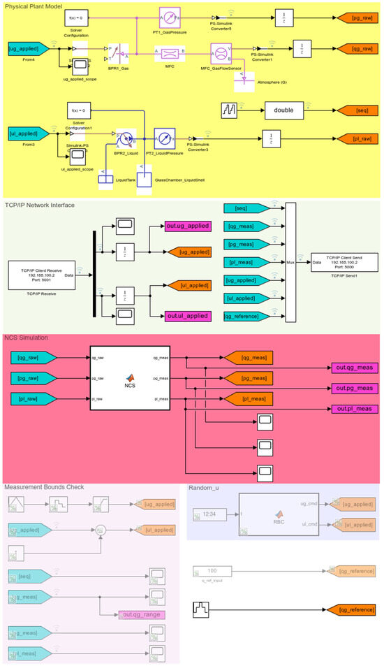
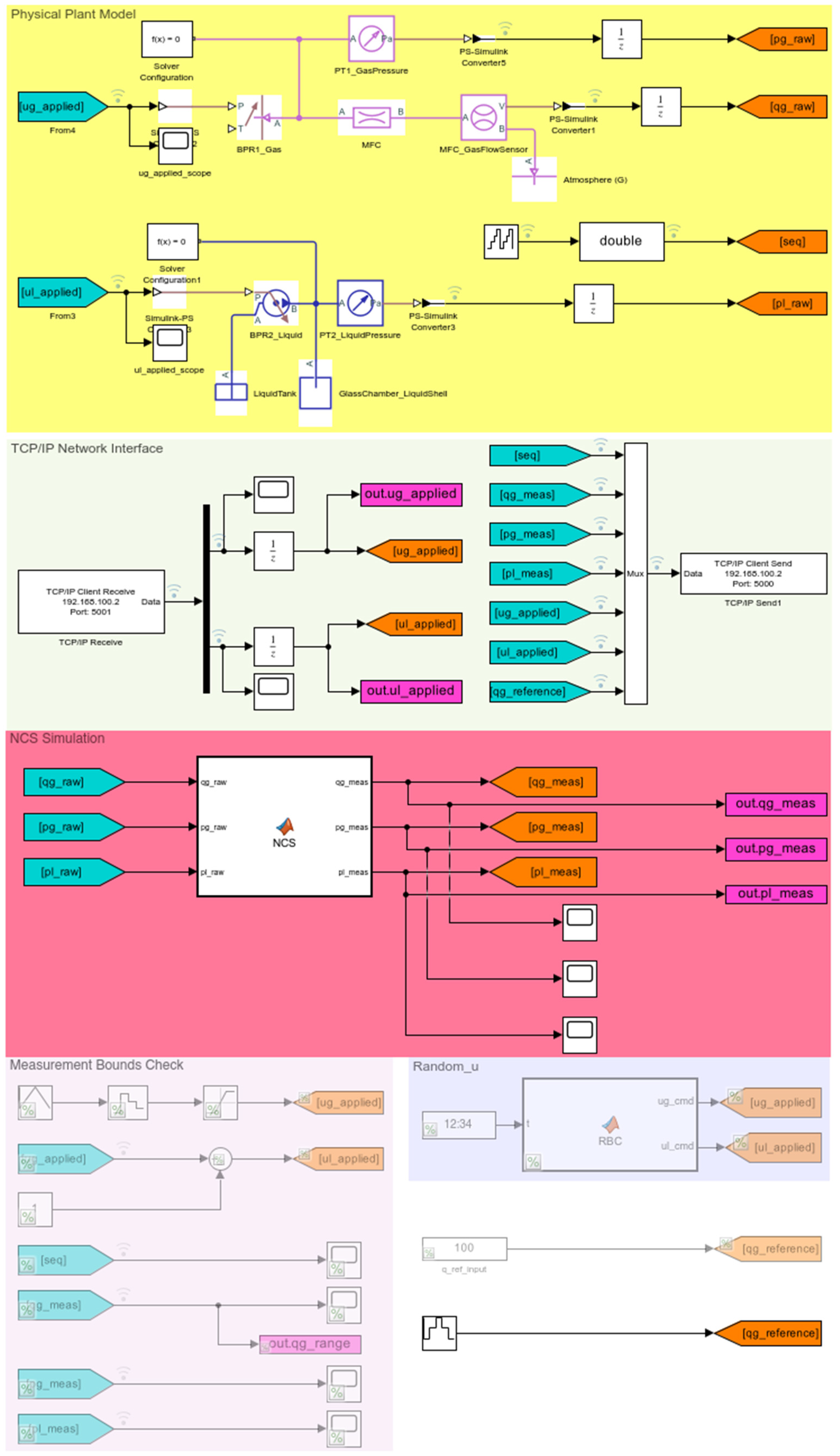
Figure 2 presents the overall structure of the Simulink-Simscape model, organized into functional regions comprising the physical plant model, the NCS nonlinear interaction simulation block, the TCP/IP communication interface and auxiliary blocks for different operating modes. Within the physical plant model region, the gas line consists of the controlled pressure source (BPR1_Gas), the pressure sensor (PT1_GasPressure), the throttling element MFC, the flowrate sensor (MFC_GasFlowSensor) and the boundary condition atmosphere. The liquid line comprises the controlled pressure source (BPR2_Liquid), the sensor (PT2_LiquidPressure), the tank (LiquidTank) and the annulus (GlassChamber_LiquidShell) representing the liquid volume surrounding the PTFE tube. Physical quantities are converted from the Simscape domain to the Simulink signal domain and logged at discrete sampling instant to form raw signals (qg_raw, pg_raw, pl_raw). The three raw signals are subsequently routed into the NCS Simulation region.
Figure 2.
Simulink-Simscape model of the gas–liquid plant and TCP/IP-based HIL architecture.
The NCS block incorporates the additional effects of differential pressure and nonlinear coupling interactions between the two phases, thereby generating measurement signals (qg_meas, pg_meas and pl_meas). These signals serve as feedback states of the plant and are transmitted to monitoring blocks and the data transmission interface. The Measurement Bounds Check region is utilized to monitor pressure commands, measured states and achievable flow ranges, thereby verifying compliance with established input pressure limits and differential pressure bounds.
Compared with the physical rig, the HIL model omits the dynamic characteristics of the motor and actuator mechanisms of the BPR valves. Instead of issuing motor-voltage, position or valve-opening commands, the GP-MPC controller generates two equivalent absolute-pressure commands, ug and ul, expressed in bar(a). These commands are held over each sampling interval and applied directly to the controlled pressure sources BPR1_Gas and BPR2_Liquid. Accordingly, no voltage-to-opening, opening-to-pressure, or other BPR actuator calibration relationship is used in the present reduced-order HIL model. This substitution enables the study to focus on the coupled gas–liquid dynamics and GP-MPC performance while leaving actuator-level dynamics and calibration outside the scope of the present HIL investigation.
The same plant model is used across three operating modes by altering command sources and enabling corresponding signal paths, while maintaining the physical structure of the dual-phase system. In data acquisition mode, the block (Random_u) utilizes the RBC function to randomly generate two commands (ug and ul) within the allowable pressure domain. These commands are applied to the plant to excite nonlinear characteristics and cross-coupling interactions between the two branches. At each sampling instant, the dataset-comprising sample index, measured states (qg_meas, pg_meas and pl_meas) and applied commands (ug and ul) are transmitted via the TCP/IP interface to be stored for GP model identification. In operating domain identification mode, the random command source is replaced by coordinated sweep signals for both gas and liquid sides. Both pressure commands are swept within the range of 0 ÷ 25 bar, while responses qg, pg and pl are recorded. After filtering out points violating pressure limits, the feasible gas-flow range is identified, serving as the basis for selecting reference values (qg_reference) in closed-loop control scenarios. In online control mode, the TCP/IP Network Interface region forms a closed loop between the Simulink-Simscape model and the Raspberry Pi 3. At each sampling instant, Simulink multiplexes the data vector [seq, qg_meas, pg_meas, pl_meas, ug_applied, ul_applied, qg_reference]. Here, seq denotes a monotonically increasing sequence number used to verify the ordering and continuity of the transmitted samples. The data vector is then transmitted to the Raspberry Pi through the TCP/IP Client Send block. The Raspberry Pi employs the trained GP models to solve the MPC optimization problem and returns two next control commands via the TCP/IP Client Receive block. These commands are held and applied to the physical model at the subsequent time step. The sequence of data acquisition, transmission, optimization and control command generation is repeated at each sampling step according to the receding-horizon strategy.
4.1.2. Randomized Input Generation and Training Data Collection
The block (Random_u) utilizes the RBC function to generate two randomized pressure commands ug_cmd and ul_cmd for collecting system identification data at a sampling time of 0.1 s. Both commands are expressed as equivalent absolute-pressure commands in bar(a) and are generated within the allowable interval of 1 − 25 bar(a), consistent with the manipulated-input definition in Equation (1). The pressure-command range is divided into several operating regions, and a target pressure-command pair is randomly selected within each region to improve data coverage. Each selected pair is maintained for a predefined time interval before the next pair is applied, thereby generating a diverse excitation dataset distributed across the entire operating range for training the GP models.
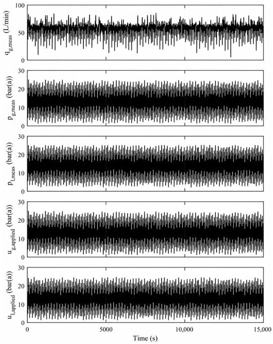
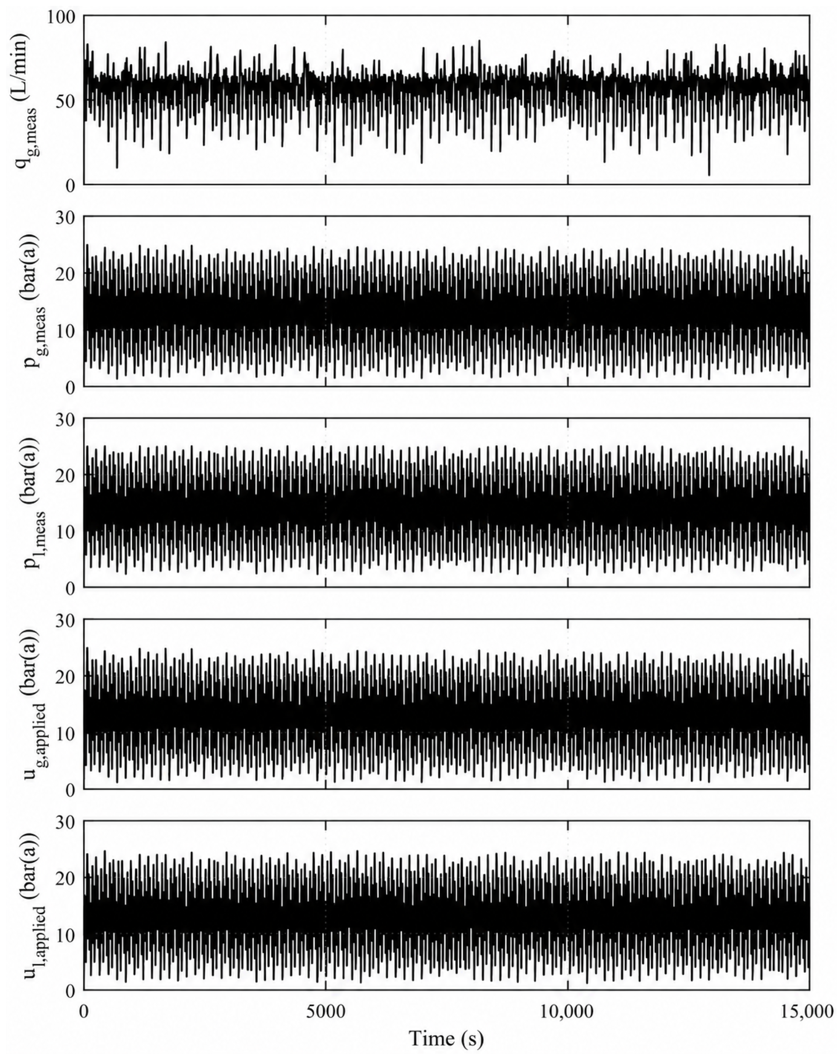
Figure 3 shows the input signals and measured responses obtained over 15,000 s of simulation. The commands (ug_applied and ul_applied) continuously explore different pressure levels across nearly the entire range of 0 ÷ 25 bar, rather than remaining confined to a narrow interval. Corresponding to this excitation, the pressures (pg_meas and pl_meas) vary over a wide band while respecting set pressure limits. The flowrate (qg_meas) also exhibits significant variation depending on the pressure state of both branches, providing coupled response data across diverse operating conditions. The signals (qg_meas, pg_meas, pl_meas, ug_applied, ul_applied) are subsequently transmitted to Raspberry Pi and logged in CSV files to build the training dataset for the GP models.
Figure 3.
Randomized equivalent pressure commands and measured responses for GP training data generation.
4.1.3. Raspberry Pi and TCP/IP Communication Configuration
Configured as a TCP server, the Raspberry Pi 3 receives data streamed from the Simulink model via the TCP/IP Client Send block. The data acquisition routine is built in Python using the TCP/IPv4 protocol, listening for incoming connections on port 5000. The Raspberry Pi software environment used for the online GP-MPC implementation consisted of Python 3.11.2, NumPy 2.4.6, SciPy 1.17.1, and scikit-learn 1.9.0. Upon establishing the connection between Simulink and Raspberry Pi, data from the HIL model are continuously streamed to the acquisition program. At each sampling instant, Simulink transmits seven signals, [seq, qg_meas, pg_meas, pl_meas, ug_applied, ul_applied, qg_reference], encoded as 64-bit floating-point values in big-endian byte order. Upon receiving and decoding the incoming data stream, the Raspberry Pi verifies the validity of each sample before logging into a CSV file for offline processing and GP model training.
4.1.4. Dataset Preprocessing and Partitioning
Following data acquisition, the CSV file is inspected for mandatory field integrity, and all required entries are cast to numeric types. Rows containing invalid values, NaN, or Inf are removed, together with consecutive duplicate samples, and the sequence index is checked for monotonicity. The resulting dataset contains 150,001 valid time-ordered samples and is partitioned chronologically, without shuffling, into contiguous training, validation, and test blocks using a 70%/15%/15% split, corresponding to 105,000, 22,500, and 22,501 raw samples, respectively. Splitting is performed before constructing the GP prediction pairs so that no transition crosses a train–validation or validation–test boundary. Within each block, the pressure-command increments are calculated in physical engineering units as ∆ug,k = ug,k − ug,k−1 and ∆ul,k = ul,k − ul,k−1. After removing the first sample required for increment calculation and the last sample for which the next-step target is unavailable, the resulting datasets contain 104,998 training pairs, 22,498 validation pairs, and 22,499 test pairs. Auxiliary fields and differential pressure are retained as analytical metadata but excluded from the GP input features. The resulting datasets are exported to gp_train.csv, gp_val.csv, and gp_test.csv. Standardization is subsequently performed using a StandardScaler fitted only to the training subset.
4.1.5. GP Model Training and Validation
Model training is conducted on the Raspberry Pi under memory-constrained execution settings. To reduce RAM usage, gp_train.csv and gp_val.csv are processed in chunks of 25,000 rows. From the 104,998 available training pairs, 1200 pairs are selected without replacement using a random seed of 42, while 5000 pairs are selected from the 22,498 available validation pairs using a seed of 1042. The three GP models use random states of 42, 43, and 44 for the gas-flow, gas-side pressure, and liquid-side pressure models, respectively. This random subsampling is performed only after the chronological train–validation–test partition has been established; therefore, it does not mix samples across temporal partitions or alter the k → k + 1 relationship within each transition pair. The independent test dataset is not subsampled and all 22,499 test pairs are retained for model evaluation. The input features are normalized using a StandardScaler fitted on the training subset and subsequently applied to the validation set. Likewise, each output target variable is individually standardized prior to model fitting. Three independent models, the gas flowrate model (GP_qg), the gas-side pressure model (GP_pg) and the liquid-side pressure model (GP_pl), are trained sequentially to predict the gas flowrate (qg,k+1), gas-side pressure (pg,k+1) and liquid-side pressure (pl,k+1) at the next sampling instant, respectively. Each GP model uses a composite kernel formed by the product of a Constant Kernel and a Matérn 5/2 kernel with Automatic Relevance Determination (ARD) length scales. A White Kernel is added to represent observation noise. The kernel hyperparameters are optimized by maximizing the log-marginal likelihood using the L-BFGS-B algorithm. After each model is trained, temporary memory is released before training the next model to reduce RAM usage on the Raspberry Pi. One-step-ahead prediction is evaluated on the validation set in batches of 250 samples. Reported evaluation metrics include R2, RMSE, MAE, mean error, maximum absolute error, average prediction standard deviation and empirical coverage probability within the 95% confidence interval. Operational parameters such as training time, validation prediction runtime, average per-sample prediction latency, and final log-marginal likelihood values are systematically logged. Finally, the three models alongside their input/output scalers are exported to gp_qg.joblib, gp_pg.joblib, and gp_pl.joblib, while a consolidated training report containing configuration details, dataset sizes, and validation metrics is saved in training_metrics.json.
Table 1 shows that all three GP models achieve high one-step-ahead prediction accuracy, with R2 values exceeding 0.99998. Values marked with an asterisk (*) were rounded to 1.000000 from 0.9999999. The gas-flow model (GP_qg) yields an RMSE of 0.035226 L/min and an empirical coverage probability of 94.94%, closely matching the nominal 95% target. The gas-side pressure model (GP_pg) and the liquid-side pressure model (GP_pl) exhibit low prediction errors, with empirical coverage probabilities of 100.00% and 99.90%, respectively. The gas-side flowrate model (GP_qg) requires the longest training duration, followed by the gas-side and liquid-side pressures (GP_pg and GP_pl). Overall, these metrics indicate that the three models effectively capture the one-step dynamics of the system across the validation dataset.
Table 1.
One-step validation performance of the trained GP Models.
Table 2 indicates that prediction errors for the gas-flow pressure model (GP_qg) gradually increase over longer prediction horizons due to recursive error accumulation. However, even at a horizon of 50 steps, the RMSE remains as low as 0.244702 L/min with an R2 of 0.9995136. Meanwhile, the gas-side and liquid-side pressures (GP_pg and GP_pl) maintain remarkably low errors and R2 values above 0.99999 across all evaluated horizons. Values marked with an asterisk (*) were rounded to 1.000000 from 0.9999999. Compared to the zero-order hold baseline, the GP models reduce RMSE by 82.752% to 99.939%, demonstrating strong multi-step predictive performance on the independent test dataset.
Table 2.
Recursive multi-step prediction performance on the independent test set.
4.1.6. Online GP-MPC
In the online control mode, the three trained GP models and their corresponding scalers are loaded onto the Raspberry Pi and converted into fast predictors to reduce computational cost. The training-dependent GP quantities are precomputed when the models are loaded, while online posterior-mean prediction still requires kernel evaluations against all retained training samples. Consequently, for the fixed regression-input dimension used in this study, the online GP inference cost increases approximately linearly with the retained training-set size. At each control interval, the current measured states and applied control inputs are used to initialize the prediction process. At each step of the prediction horizon, the GP input vector is constructed from the predicted states, control inputs and corresponding input increments. The posterior means of the three GP models are then used to predict qg, pg and pl at the next step. This procedure is recursively repeated to generate the predicted state trajectory over the entire prediction horizon. The GP input vector excludes the reference gas flowrate qg_reference, which serves solely as the setpoint in the MPC optimization problem. In addition, the difference between the measured qg and its previous one-step prediction is used to update a bias correction term, thereby reducing the influence of local model errors on flowrate tracking performance. The online predictor is configured with a prediction horizon of Np = 3 and a control horizon of Nc = 2. The first two input increments are treated as decision variables, while the control inputs are held constant beyond the control horizon. For each candidate control sequence, the three GP models are recursively evaluated to predict the system response while checking the constraints on ug, ul, input variations and the pressure difference between pg and pl. Feasible predicted trajectories are evaluated using an objective function that considers the qg tracking error, pressure difference, control variation, terminal error and convergence behavior. The control sequence with the minimum objective value is then selected to update the control inputs for the next sampling interval.
The online gas-flow bias correction is implemented additively to the GP gas-flow prediction rather than as an additional MPC cost term. The bias estimator uses an update coefficient of α = 0.02, with both the innovation and bias limited to ±1 L/min. Bias updating begins after 30 control packets and is enabled only when the gas-flow tracking error is within 2 L/min. Computational timing was evaluated from the recorded HIL execution data rather than inferred from the HIL sampling interval. Across 7501 control packets, the mean and maximum MPC solution times were tsolve,mean = 0.1045 s and tsolve,max = 1.1616 s, respectively. These measurements show that the present Raspberry Pi 3 implementation does not consistently satisfy a 0.1 s wall-clock computational deadline. Accordingly, Ts = 0.1 s is interpreted as the HIL sampling interval rather than as a demonstrated 10 Hz real-time execution guarantee. Separate TCP/IP transmission latency was not instrumented in the recorded logger, and no per-cycle socket timeout was configured; therefore, independent communication-latency and timeout values are not reported.
4.1.7. Determination of the Feasible Gas-Flow Range
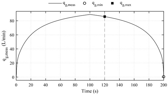
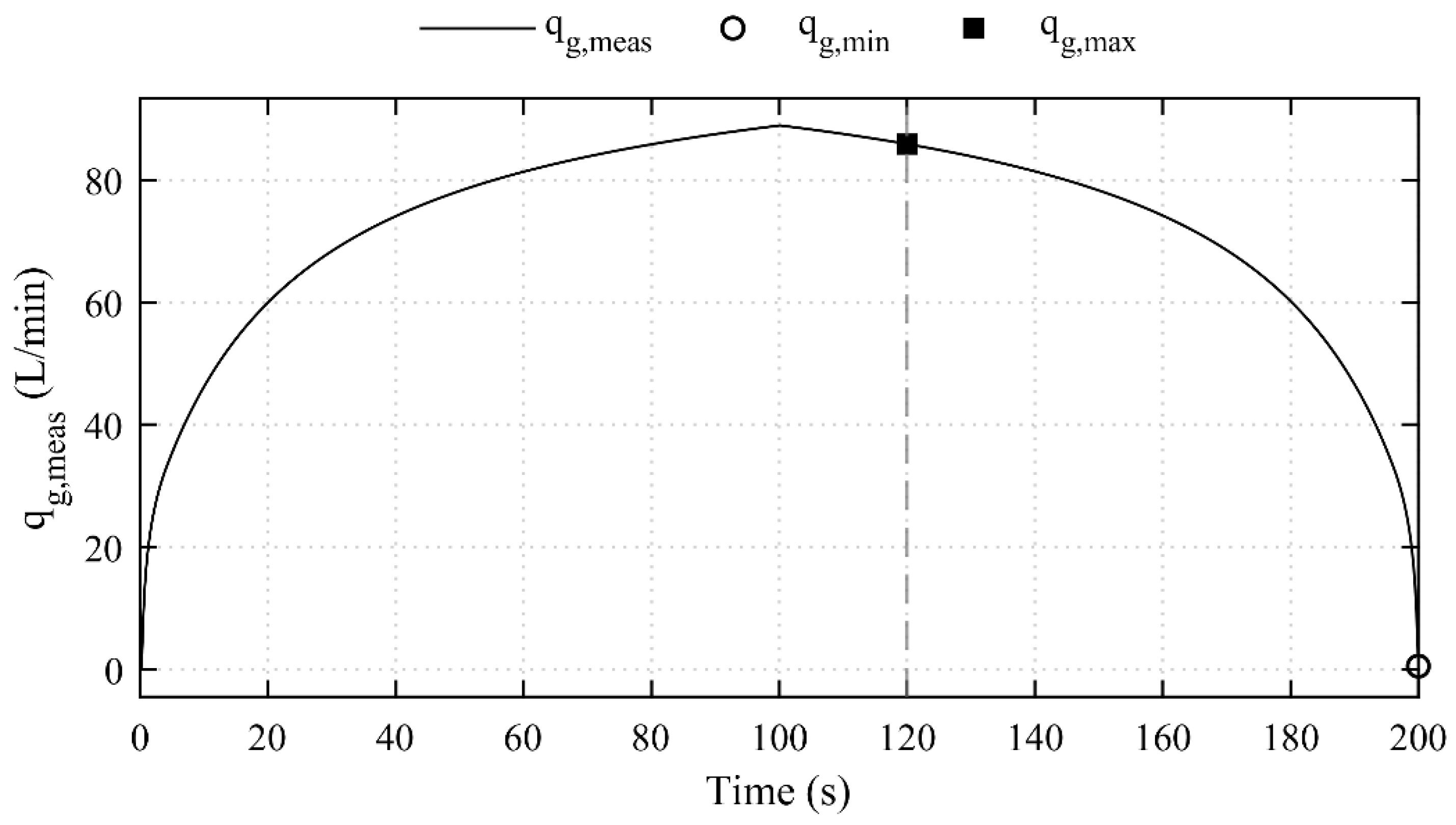
The feasible gas-flow range of the model is identified using an input sweep configuration. In this test, pressure commands ug and ul are swept in a coordinated fashion across the allowable operating envelope, while maintaining absolute pressure bounds and the differential pressure constraint |pg − pl| ≤ 0.85 bar. The simulation duration is set to 200 s and the qg_meas response is recorded throughout.
Figure 4 illustrates the variation in qg_meas during the pressure-command sweep. The gas flowrate increases as the pressure commands approach the upper region of their specified range, reaches its maximum near the midpoint of the sweep and then decreases as the inputs return toward their lower limits. The maximum value is determined over the entire simulation interval from 0 ÷ 200 s, whereas the minimum value is determined along the descending branch after the maximum to exclude the influence of the initial conditions. The results show that qg_meas reaches a maximum of 88.915 L/min at t = 100.1 s and a minimum of 0.540 L/min at t = 200.0 s, corresponding to a variation range of 88.374 L/min. Therefore, the interval of 0.540 ÷ 88.915 L/min is considered the observed flowrate range of the model under the applied pressure-command sweep and specified pressure limits.
Figure 4.
Observed range of the measured gas flowrate during the pressure-command scan.
4.2. Closed-Loop GP-MPC Performance Evaluation Under HIL
4.2.1. Scenario 1: Evaluation of Tracking Capability at Fixed Reference Flowrates
The first scenario is designed to evaluate the gas-flow tracking capability of the GP-MPC controller at distinct operating points within the HIL setup. In experimental studies on gas–liquid two-phase flows, Radhi et al. investigated gas–water systems at gas flowrate levels of 8.3, 16.6, and 25 L/min [28]. Based on these benchmarks, these three flowrates are selected as constant setpoints in this simulation scenario. Three independent tests are conducted, where the reference flowrate remains constant throughout each run. The identical GP-MPC configuration and operational constraints detailed in previous sections are applied across all cases to assess and compare tracking performance across operating regimes.
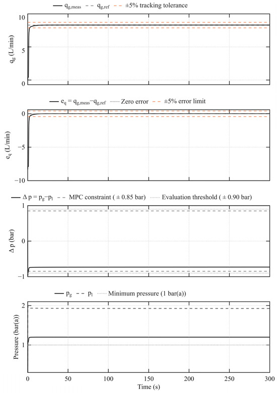
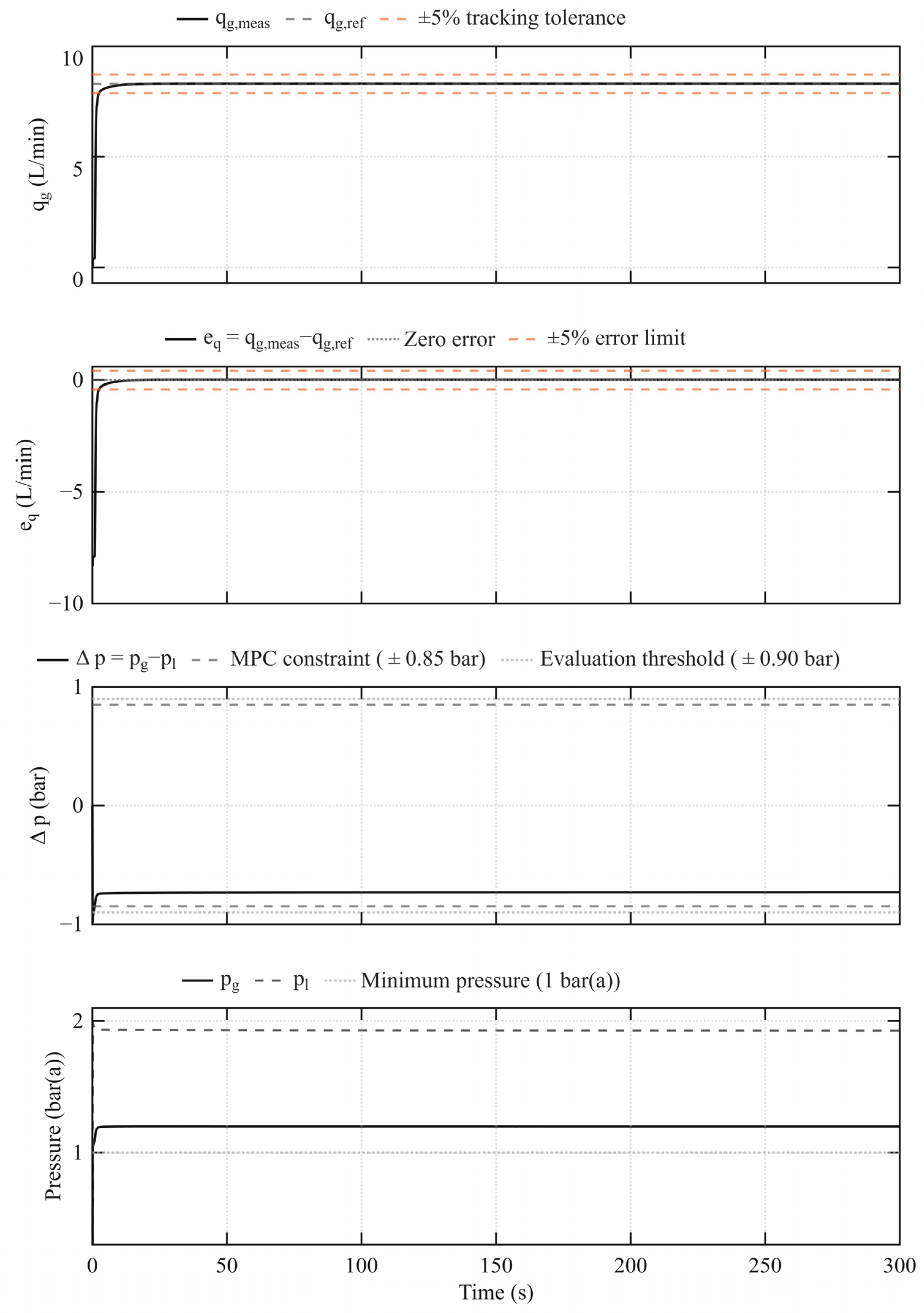
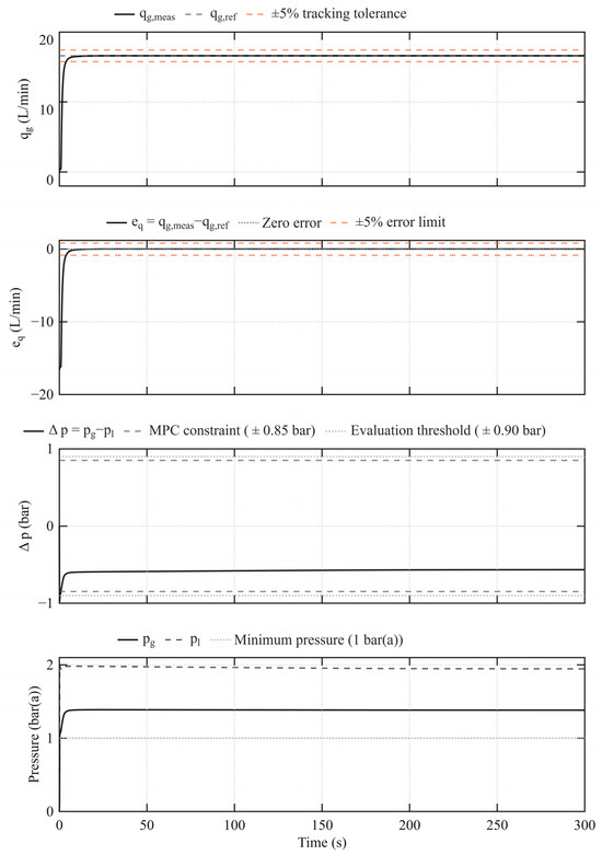
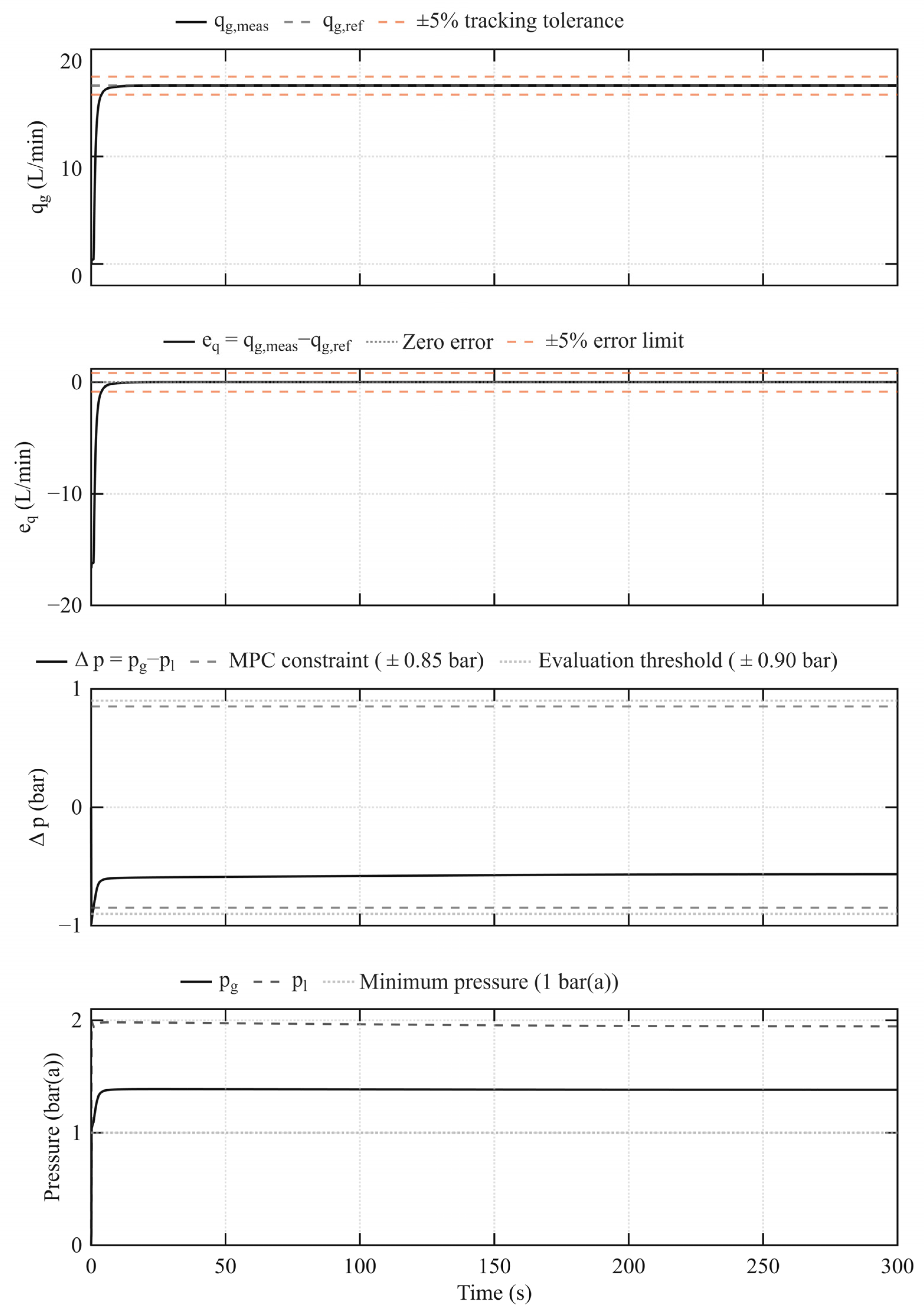
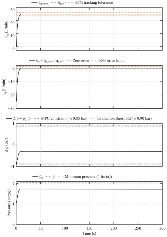
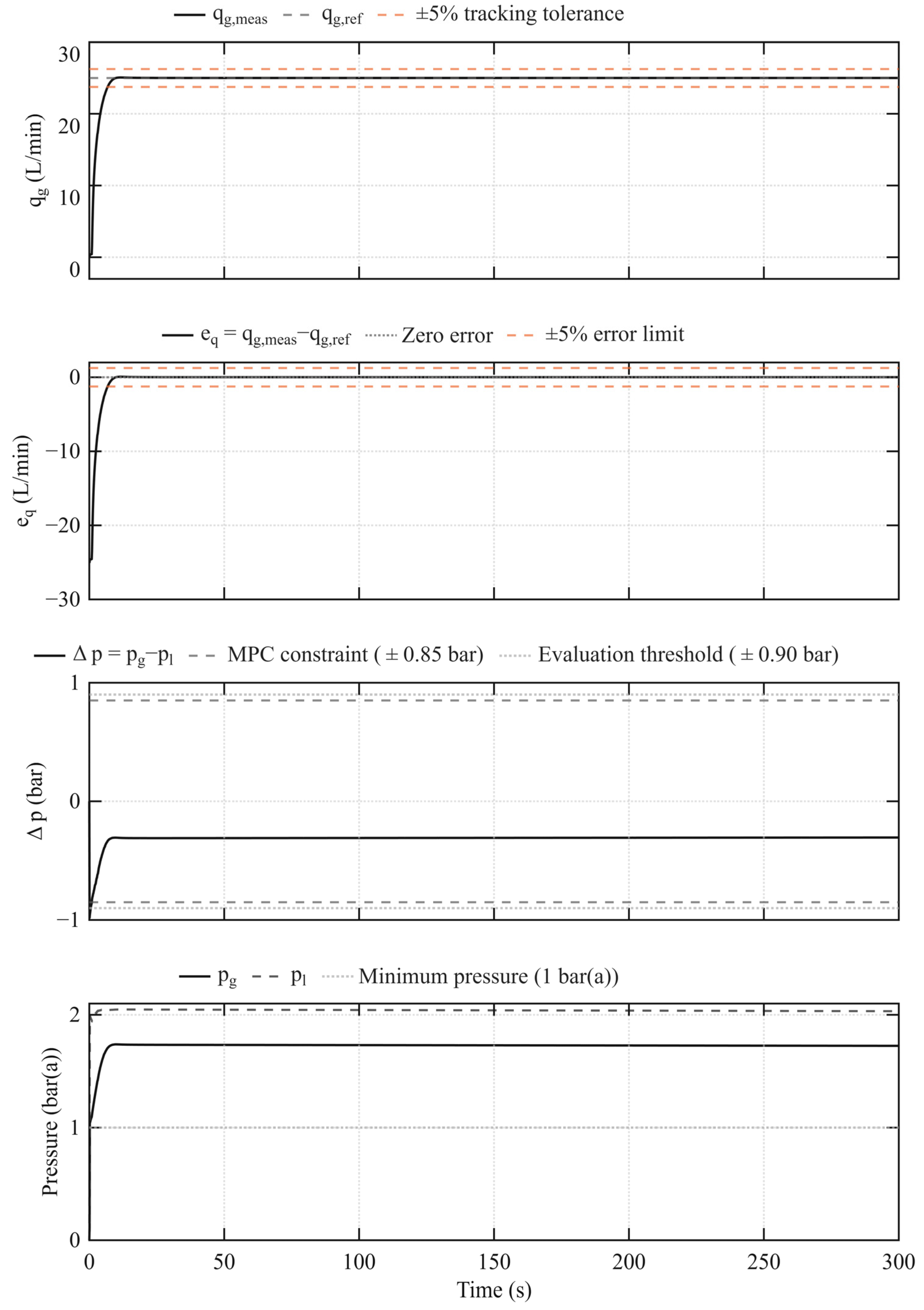
Figure 5, Figure 6 and Figure 7 illustrate the closed-loop responses of the physics-based gas–liquid plant model implemented in MATLAB/Simulink-Simscape under GP-MPC regulation for fixed reference flowrates of 8.3, 16.6 and 25 L/min, while Table 3 summarizes key quantitative performance metrics. Overall, GP-MPC effectively drives the gas flowrate qg from the initial zero state to the setpoint, maintaining tight stability around the specified reference flowrates across all tested operating points. Following the transient phase, the responses remain well within a ±5% error band around the reference without noticeable steady-state oscillations. These results confirm that the integrated GP model provides reliable predictions, enabling the MPC controller to calculate accurate control signals across diverse operating conditions.
Figure 5.
Closed-loop GP-MPC response for a gas-flow reference of 8.3 L/min.
Figure 6.
Closed-loop GP-MPC response for a gas-flow reference of 16.6 L/min.
Figure 7.
Closed-loop GP-MPC response for a gas-flow reference of 25 L/min.
Table 3.
Summary of GP-MPC performance at fixed gas flowrate references.
Performance differences across the three cases become clearer through the metrics summarized in Table 3. Settling time increases from 2.5 s at reference flowrate of 8.3 L/min to 3.9 s at 16.6 L/min and 6.8 s at 25 L/min. This trend indicates that higher flowrate targets requiring larger state transitions from qg = 0 demand longer settling periods for the controller to bring the system into steady state. However, longer settling times have a little effect on steady-state accuracy with relative steady-state errors of 0.121%, 0.053% and 0.030%, respectively. Furthermore, overshooting across all three operating points remains negligible (0.144%, 0.065% and 0.285%). Thus, despite a slower response at 25 L/min, there is no significant trade-off between convergence speed and steady-state precision within the tested operating range.
Table 3 shows that the overall RMSE increases with the reference flowrate across the three tested operating points of 8.3, 16.6, and 25 L/min. This increase has little effect on steady-state tracking performance. Because the RMSE is calculated over the entire simulation duration, it includes the startup transitions from 0 L/min to 8.3, 16.6 and 25 L/min. At higher reference flowrate, the initial gas flowrate tracking error is larger and the settling interval becomes longer, resulting in a greater contribution of the transient response to the accumulated squared error. This interpretation is consistent with the small steady-state errors reported in Table 3. Therefore, the overall RMSE reflects both transient tracking performance and steady-state accuracy rather than steady-state precision alone.
Figure 5, Figure 6 and Figure 7 evaluate the system behavior with respect to the differential-pressure operating constraint, |∆p| ≤ 0.85 bar. During startup initialization, all three fixed-reference cases exhibit a brief peak absolute differential pressure of approximately 0.982 bar. This peak exceeds the 0.85-bar MPC operating constraint by approximately 0.132 bar and the 0.90-bar evaluation threshold by approximately 0.082 bar. The 0.90-bar threshold is exceeded for four consecutive samples at the 8.3 L/min reference and five consecutive samples at the 16.6 and 25 L/min references, corresponding to approximately 0.4 s and 0.5 s, respectively, at the 0.1 s sampling interval. After the startup transient, |∆p| decreases below the 0.85-bar operating constraint and remains within this limit for the remainder of each fixed-reference test. The nearly identical startup peaks observed across the three reference cases indicate that this transient is primarily associated with the initial conditions and controller initialization rather than the reference-flow magnitude. Because the differential pressure constraint is enforced on the nominal trajectory predicted using the GP posterior mean, this plant-side startup violation also shows that nominal predicted constraint satisfaction does not guarantee satisfaction of the same bound by the HIL plant.
4.2.2. Scenario 2: Evaluation of Tracking Performance Under Stepwise Reference Changes
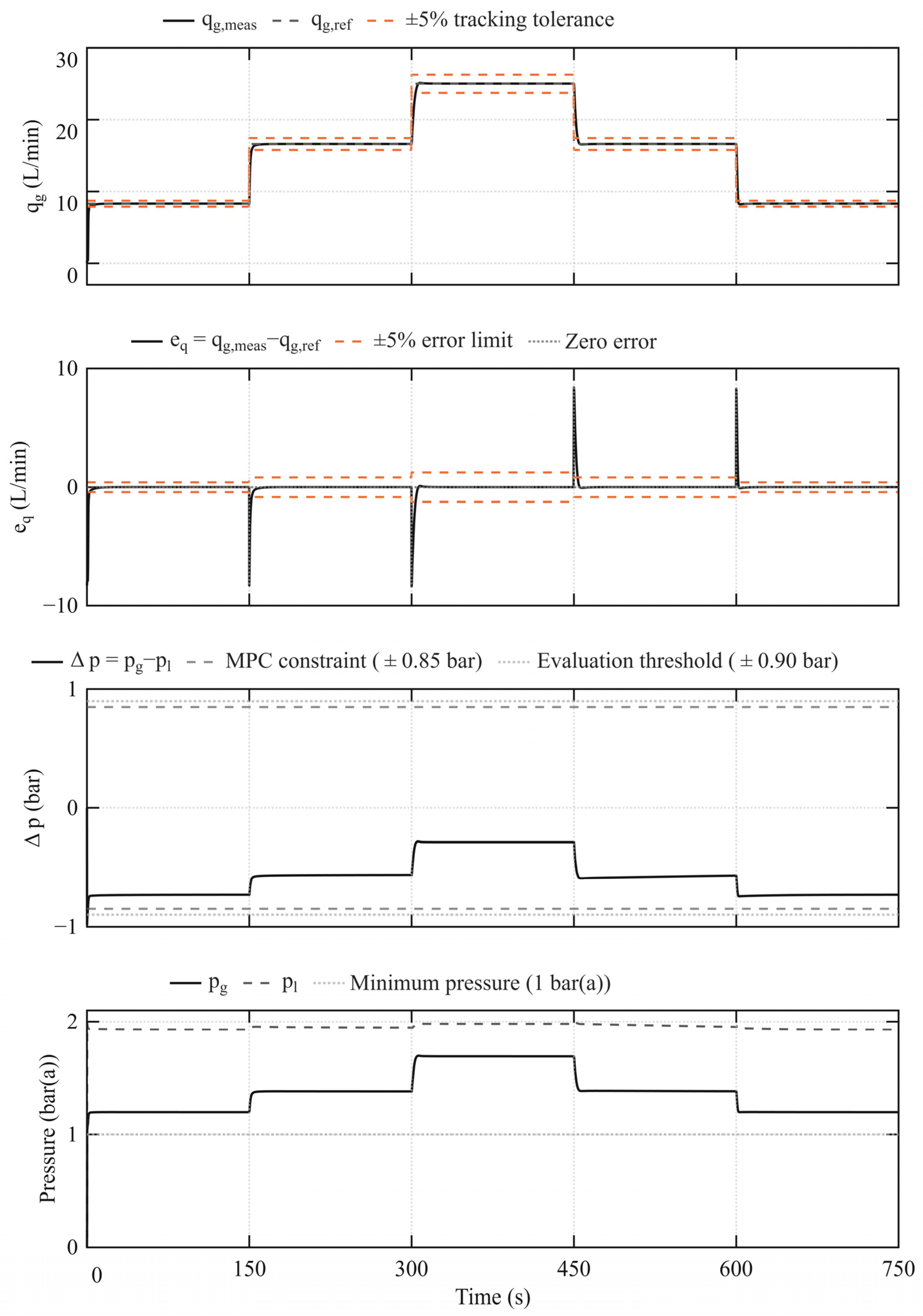
Following the fixed setpoint evaluations in Scenario 1, Scenario 2 investigates the dynamic tracking response of the GP-MPC controller under stepwise setpoint changes during continuous operation. Unlike Scenario 1, this test is conducted continuously without resetting system states during setpoint transitions. The reference flowrates of 8.3, 16.6 and 25 L/min are used for consistency. Initially, the reference flowrate is set at 8.3 L/min for 150 s, then stepped up to 16.6 L/min (150 ÷ 300 s) and 25 L/min (300 ÷ 450 s). In the second half of the run, setpoints are stepped down to 16.6 L/min (450 ÷ 600 s) and back to 8.3 L/min (600 ÷ 750 s). This setup generates four consecutive step transitions (two step-ups and two step-downs), with each operating point maintained for 150 s. This simulation is used to assess transient response, settling time, tracking error, adaptation to bidirectional reference changes and satisfaction of the operating constraints.
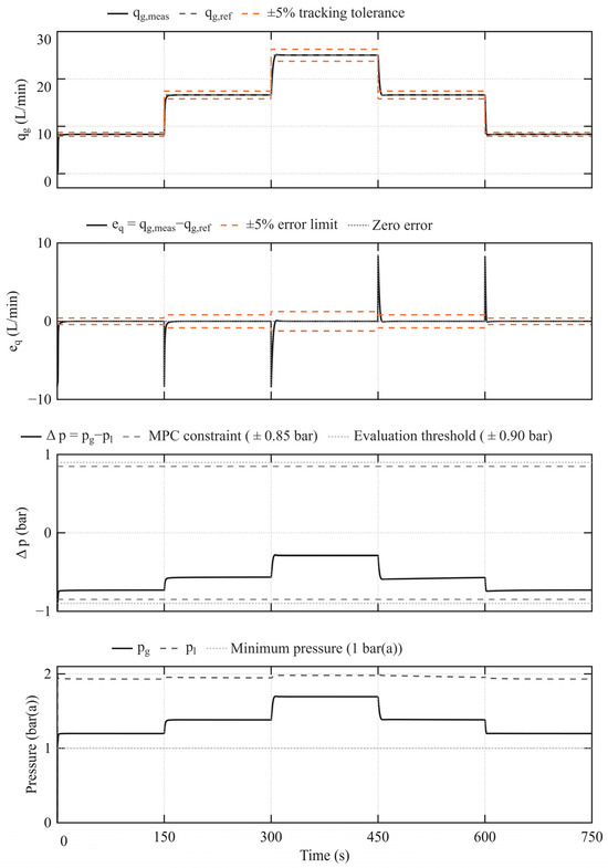
Closed-loop responses of the physics-based gas–liquid plant model implemented in MATLAB/Simulink-Simscape during the stepwise test are shown in Figure 8, with segment-by-segment quantitative metrics summarized in Table 4. The GP-MPC scheme exhibits consistent tracking across both upward and downward setpoint transitions, achieving an overall 750 s RMSE of 0.654 L/min and MAE of 0.091 L/min. After each setpoint change, the gas flowrate converges rapidly to the target value without lingering oscillations. For the four transitions, 5% settling times are 2.3, 3.7, 3.5 and 1.9 s, respectively, while steady-state errors across all segments remain within 0.026 ÷ 0.121%. The transient overshoot or undershoot values for four changes are 0.061%, 0.406%, 0.312% and 1.069%. Directional asymmetry is observed at the 16.6 L/min setpoint: stepping up from 8.3 L/min requires 2.3 s to settle, whereas stepping down from 25 L/min requires 3.5 s. However, steady-state errors remain virtually identical (0.053% and 0.056%), indicating that transition direction primarily influences transient speed rather than steady-state precision. For the differential-pressure response, the maximum value of |∆p| = 0.9823 bar occurs during the initial startup period, exceeding both the 0.85-bar MPC operating constraint and the 0.9-bar evaluation threshold. No further violations of the 0.85-bar MPC operating constraints are observed during the subsequent step transitions at 150, 300, 450, and 600 s, where the corresponding |∆pmax| values are 0.731, 0.564, 0.593, and 0.744 bar, respectively.
Figure 8.
Closed-loop response of the GP-MPC under stepwise gas flow reference changes.
Table 4.
GP-MPC performance under stepwise gas flow reference changes.
5. Discussion
This study developed a fully data-driven GP-MPC framework for coordinated gas flowrate and pressure regulation in an interacting nonlinear gas–liquid system. Three independent GP models with Matérn 5/2 kernels were trained to predict the gas flowrate, gas-side pressure and liquid-side pressure from the current states, two equivalent pressure commands and their increments. The GP mean predictions were recursively propagated within the MPC formulation, which incorporated gas flowrate tracking, differential-pressure regulation, control variation, terminal tracking error, input constraints and online flowrate bias correction. The complete GP inference and optimization procedure was executed on a Raspberry Pi 3 and connected through TCP/IP to a MATLAB/Simulink-Simscape plant model with a sampling period of 0.1 s.
The model validation confirmed that all three GP models achieved one-step-ahead values above 0.99998. The gas flowrate model retained an RMSE of 0.2447 L/min over a 50-step recursive prediction horizon, indicating that the learned dynamics remained sufficiently accurate for short horizon online prediction. At fixed reference flowrates of 8.3, 16.6 and 25 L/min, the GP-MPC controller achieved settling times ranging from 2.5 to 6.8 s, relative steady-state errors below 0.121% and overshoots below 0.285%. During continuous bidirectional reference changes, the controller achieved an overall RMSE of 0.654 L/min and MAE of 0.091 L/min, with settling times between 1.9 and 3.7 s. A brief differential-pressure constraint violation occurred during startup, reaching approximately 0.982 bar. After this startup transient, no further violations of the 0.85-bar MPC operating constraint were observed during the subsequent reference transitions. This startup violation indicates that enforcing the constraint on the nominal GP-mean prediction does not guarantee plant-side constraint satisfaction.
Overall, these findings demonstrate the computational execution of the multivariable GP-MPC framework on Raspberry Pi 3 hardware within the present HIL configuration. They should not be interpreted as validation of practical deployment or performance on the physical gas–liquid apparatus. The gas–liquid plant is simulated rather than physical, the equivalent pressure commands omit the actuator dynamics of the motorized back-pressure regulators, and the controller propagates only the GP predictive mean without accounting for predictive uncertainty. Consequently, the present results do not provide probabilistic constraint guarantees or establish performance under physical experimental conditions. Future work will therefore investigate improved startup initialization and reference shaping, soft-constraint formulations, and uncertainty-aware or chance-constrained MPC formulations, together with incorporation of actuator dynamics and experimental validation on the physical gas–liquid system. Additional validation procedures, including residual autocorrelation analysis, repeated training under different random seeds, and comparative statistical testing, will also be conducted to further assess model consistency, robustness, and statistical significance.
Author Contributions
Conceptualization, H.N.N., C.T.T. and V.T.D.; methodology, V.T.D.; software, H.N.N. and H.D.H.; validation, H.H.N.; formal analysis, H.H.N.; investigation, C.T.T.; resources, C.T.T.; data curation, H.D.H.; writing—original draft preparation, H.N.N. and C.T.T.; writing—review and editing, V.T.D.; visualization, H.N.N. and H.D.H.; supervision, T.T.N.; project administration, H.H.N.; funding acquisition, T.T.N. All authors have read and agreed to the published version of the manuscript.
Funding
This research was funded by Vietnam National University Ho Chi Minh City (VNU-HCM), grant number CB2025-20-15.
Institutional Review Board Statement
Not applicable.
Informed Consent Statement
Not applicable.
Data Availability Statement
The original contributions presented in the study are included in the article, further inquiries can be directed to the corresponding author/s.
Acknowledgments
This research is funded by Vietnam National University Ho Chi Minh City (VNU-HCM) under a project within the framework of the program titled “Strengthening the capacity for education and basic scientific research integrated with strategic technologies at VNU-HCM, aiming to achieve advanced standards comparable to regional and global levels during the 2025–2030 period, with a vision toward 2045”, grant number CB2025-20-15.
Conflicts of Interest
The authors declare no conflicts of interest.
Abbreviations
The following abbreviations are used in this manuscript:
| BPR | Back-Pressure Regulator |
| GP | Gaussian Process |
| GP-MPC | Gaussian Process-Based Model Predictive Control |
| HIL | Hardware-in-the-Loop |
| MAE | Mean Absolute Error |
| MFC | Mass Flow Controller |
| MIMO | Multiple-Input Multiple-Output |
| MPC | Model Predictive Control |
| PT | Pressure Transmitter |
| R2 | Coefficient of Determination |
| RMSE | Root Mean Square Error |
| TCP/IP | Transmission Control Protocol/Internet Protocol |
References
- Gabelman, A.; Hwang, S.-T. Hollow Fiber Membrane Contactors. J. Memb. Sci. 1999, 159, 61–106. [Google Scholar] [CrossRef] [Scilit]
- Li, M.; Zhu, Z.; Zhou, M.; Jie, X.; Wang, L.; Kang, G.; Cao, Y. Removal of CO2 from Biogas by Membrane Contactor Using PTFE Hollow Fibers with Smaller Diameter. J. Memb. Sci. 2021, 627, 119232. [Google Scholar] [CrossRef] [Scilit]
- Feng, S.; Zhong, Z.; Wang, Y.; Xing, W.; Drioli, E. Progress and Perspectives in PTFE Membrane: Preparation, Modification, and Applications. J. Memb. Sci. 2018, 549, 332–349. [Google Scholar] [CrossRef] [Scilit]
- Dat, P.; Pham, T.; Toai, T.; Duong, V.; Nguyen Huy, H. Adaptive Sliding Mode Control for a Blower-Based Breathing Simulator with Unknown and Time-Varying Airway Resistance and Compliance; IEEE: Piscataway, NJ, USA, 2024. [Google Scholar]
- Truong, C.T.; Phan, T.D.; Tran, M.T.; Nguyen, H.H.; Duong, V.T.; Nguyen, T.T. Disturbance Observer-Based Sliding Mode Control for Ventilation Blower-Based Systems: Controller Design and Simulation. Int. J. Online Biomed. Eng. iJOE 2025, 21, 132–151. [Google Scholar] [CrossRef] [Scilit]
- Le, N.; Toai, T.; Duong, V.; Nguyen, T.; Nguyen Huy, H. A Hybrid Model Reference Adaptive and Regressive-Form Sliding Mode Control in Discrete Domain: Robustness Under System Uncertainty. Eng. Rep. 2025, 7, e70527. [Google Scholar] [CrossRef] [Scilit]
- Grancharova, A.; Johansen, T.A.; Kocijan, J. Explicit Model Predictive Control of Gas–Liquid Separation Plant via Orthogonal Search Tree Partitioning. Comput. Chem. Eng. 2004, 28, 2481–2491. [Google Scholar] [CrossRef] [Scilit][Green Version]
- Likar, B.; Kocijan, J. Predictive Control of a Gas–Liquid Separation Plant Based on a Gaussian Process Model. Comput. Chem. Eng. 2007, 31, 142–152. [Google Scholar] [CrossRef] [Scilit]
- Pedersen, T.; Aarsnes, U.J.F.; Godhavn, J.-M. Flow and Pressure Control of Underbalanced Drilling Operations Using NMPC. J. Process Control 2018, 68, 73–85. [Google Scholar] [CrossRef] [Scilit]
- Adaze, E.; Al-Sarkhi, A.; Badr, H.M.; Elsaadawy, E. Current Status of CFD Modeling of Liquid Loading Phenomena in Gas Wells: A Literature Review. J. Pet. Explor. Prod. Technol. 2019, 9, 1397–1411. [Google Scholar] [CrossRef] [Scilit]
- Ullmann, A.; Brauner, N. Closure Relations for Two-Fluid Models for Two-Phase Stratified Smooth and Stratified Wavy Flows. Int. J. Multiph. Flow 2006, 32, 82–105. [Google Scholar] [CrossRef] [Scilit]
- Schoukens, J.; Ljung, L. Nonlinear System Identification: A User-Oriented Road Map. IEEE Control Syst. Mag. 2019, 39, 28–99. [Google Scholar] [CrossRef] [Scilit]
- Kocijan, J.; Girard, A.; Banko, B.; Murray-Smith, R. Dynamic Systems Identification with Gaussian Processes. Math. Comput. Model. Dyn. Syst. 2005, 11, 411–424. [Google Scholar] [CrossRef] [Scilit]
- Rasmussen, C.E.; Williams, C.K.I. Gaussian Processes for Machine Learning; The MIT Press: Cambridge, MA, USA, 2005; ISBN 9780262256834. [Google Scholar]
- Kocijan, J.; Murray-Smith, R.; Rasmussen, C.E.; Girard, A. Gaussian Process Model Based Predictive Control. In Proceedings of the 2004 American Control Conference, Boston, MA, USA, 30 June 2004–2 July 2004; IEEE: Piscataway, NJ, USA, 2004; Volume 3, pp. 2214–2219. [Google Scholar]
- Hewing, L.; Kabzan, J.; Zeilinger, M.N. Cautious Model Predictive Control Using Gaussian Process Regression. IEEE Trans. Control Syst. Technol. 2019, 28, 2736–2743. [Google Scholar] [CrossRef] [Scilit]
- Bradford, E.; Imsland, L.; Zhang, D.; del Rio Chanona, E.A. Stochastic Data-Driven Model Predictive Control Using Gaussian Processes. Comput. Chem. Eng. 2020, 139, 106844. [Google Scholar] [CrossRef] [Scilit]
- Koller, T.; Berkenkamp, F.; Turchetta, M.; Krause, A. Learning-Based Model Predictive Control for Safe Exploration. In Proceedings of the 2018 IEEE Conference on Decision and Control (CDC), Miami, FL, USA, 17–19 December 2018; IEEE: Piscataway, NJ, USA, 2018; pp. 6059–6066. [Google Scholar]
- Maiworm, M.; Limon, D.; Findeisen, R. Online Learning-Based Model Predictive Control with Gaussian Process Models and Stability Guarantees. Int. J. Robust. Nonlinear Control 2021, 31, 8785–8812. [Google Scholar] [CrossRef] [Scilit]
- Hewing, L.; Wabersich, K.P.; Menner, M.; Zeilinger, M.N. Learning-Based Model Predictive Control: Toward Safe Learning in Control. Annu. Rev. Control Robot. Auton. Syst. 2020, 3, 269–296. [Google Scholar] [CrossRef] [Scilit]
- Janssen, N.; Kools, L.; Antunes, D. Embedded Learning-Based Model Predictive Control for Mobile Robots Using Gaussian Process Regression. In Proceedings of the 2020 American Control Conference (ACC), Denver, CO, USA, 1–3 July 2020; IEEE: Piscataway, NJ, USA, 2020. [Google Scholar]
- Lahr, A.; Näf, J.; Wabersich, K.P.; Frey, J.; Siehl, P.; Carron, A.; Diehl, M.; Zeilinger, M.N. L4acados: Learning-Based Models for Acados, Applied to Gaussian Process-Based Predictive Control. IEEE Trans. Control Syst. Technol. 2026, 34, 1091–1105. [Google Scholar] [CrossRef] [Scilit]
- Lahr, A.; Zanelli, A.; Carron, A.; Zeilinger, M.N. Zero-Order Optimization for Gaussian Process-Based Model Predictive Control. Eur. J. Control 2023, 74, 100862. [Google Scholar] [CrossRef] [Scilit]
- Scampicchio, A.; Arcari, E.; Lahr, A.; Zeilinger, M.N. Gaussian Processes for Dynamics Learning in Model Predictive Control. Annu. Rev. Control 2025, 60, 101034. [Google Scholar] [CrossRef] [Scilit]
- Prajapat, M.; Lahr, A.; Köhler, J.; Krause, A.; Zeilinger, M.N. Towards Safe and Tractable Gaussian Process-Based MPC: Efficient Sampling within a Sequential Quadratic Programming Framework. In Proceedings of the 2024 IEEE 63rd Conference on Decision and Control (CDC), Milan, Italy, 16–19 December 2024; IEEE: Piscataway, NJ, USA, 2024; pp. 7458–7465. [Google Scholar]
- Hewing, L.; Liniger, A.; Zeilinger, M.N. Cautious Nmpc with Gaussian Process Dynamics for Autonomous Miniature Race Cars. In Proceedings of the 2018 European control conference (ECC), Limassol, Cyprus, 12–15 June 2018; IEEE: Piscataway, NJ, USA, 2018; pp. 1341–1348. [Google Scholar]
- Cao, G.; Lai, E.M.-K.; Alam, F. Gaussian Process Model Predictive Control of an Unmanned Quadrotor. J. Intell. Robot. Syst. 2017, 88, 147–162. [Google Scholar] [CrossRef] [Scilit]
- Radhi, D.; Mohsen, A.M.H.; Abdulkadhim, A. Experimental Investigation of Two-Phase Fluid Flow over a Rectangular Obstructions Located inside Enlarged Rectangular Channel. Math. Model. Eng. Probl. 2019, 6, 183–187. [Google Scholar] [CrossRef] [Scilit]

Disclaimer/Publisher’s Note: The statements, opinions and data contained in all publications are solely those of the individual author(s) and contributor(s) and not of MDPI and/or the editor(s). MDPI and/or the editor(s) disclaim responsibility for any injury to people or property resulting from any ideas, methods, instructions or products referred to in the content. |
© 2026 by the authors. Licensee MDPI, Basel, Switzerland. This article is an open access article distributed under the terms and conditions of the Creative Commons Attribution (CC BY) license.