Parameter Efficient Asymmetric Feature Pyramid for Early Wildfire Detection

Abstract

This work addresses the need for high recall with low false alarms in early wildfire monitoring and presents AsymmetricFPN, an asymmetric feature pyramid centered on parameter efficiency. Within a RetinaNet framework, we replace Smooth L1 with CIoU to stabilize small object localization and perform lightweight post-fusion refinement at key sites where multiscale context is already integrated. We construct a composite dataset with perceptual hash deduplication and evaluate all models under a unified protocol. Results show that AsymmetricFPN achieves mAP@0.5 of 85.5% and recall of 81.2%, reaches mAP@[0.5:0.95] of 44.0%, attains the highest parameter efficiency (η = 2.34), and delivers 26.10 FPS end-to-end. In addition, the localization-aware efficiency, defined as η@[0.5:0.95] = mAP@[0.5:0.95]/Params(M), reaches ≈ 1.21 and is the highest under the unified protocol. Compared with representative one stage baselines under identical settings, it provides comparable core detection capability with fewer parameters and fewer false positives in confounding backgrounds such as water glare and sunset. We conclude that task-oriented asymmetric architecture with lightweight post-fusion refinement offers a reusable route to reconcile accuracy, efficiency, and deployment cost for practical wildfire detection.

1. Introduction

Globally, the frequency and intensity of forest wildfires have increased due to warming and extreme drought, causing substantial environmental and economic losses and posing a pressing challenge to humanity [1,2]. For forest fire detection, conventional lookout towers, optical remote sensing, and ground IoT systems suffer from limited resolution, occlusion, and noise, and therefore cannot meet the requirements of early, stable monitoring with low false alarms [3]. Satellite sensing fails under cloud cover and incurs considerable latency [4]. Ground sensing networks also face high deployment and maintenance costs, energy constraints, and frequent false positives [5]. Accordingly, data-driven, vision-based deep learning methods have become a mainstream approach for automated early wildfire detection on imagery acquired by satellites, UAVs, and ground cameras. However, scenes with many small objects and backgrounds with strong appearance variation, such as sunsets, specular highlights on water, and clouds, pose high demands on recall and precision. The joint requirements for low false alarm rates and deployability are also stringent. Existing research largely follows two routes. The first is accuracy-oriented and increases robustness by injecting multiscale features and attention into the backbone and neck, or by adopting transformer based paradigms. For example, Zhu et al. [6] introduce AgentAttention and EMA attention into YOLOv8, employ BiFormer for adaptive multiscale fusion, replace C2f with local convolution, and strengthen context interaction to improve multiscale detection accuracy in complex forest scenes through stronger feature representations. Ramos et al. [7] perform heavy hyperparameter optimization on YOLOv8, first screening sensitivities with OAT and then using random search to optimize learning rate, momentum, IoU thresholds, label assignment, and augmentation, achieving significant gains without structural changes through longer training and higher input resolution. Huang et al. [8] propose an end-to-end model based on Deformable DETR, combining a multiscale contrastive context module (MCCL), dense pyramid pooling (DPPM), and enhanced query interactions to improve small smoke detection via stronger global modeling and multiscale fusion. Park et al. [9] present a StyleGAN2 ADA synthetic augmentation pipeline that generates large scale diverse smoke samples, and train YOLOv8 and RT DETR with strong augmentation for extended periods, trading data and training intensity for higher accuracy and robustness in challenging scenes. Bakirci et al. [10] adopt the GELAN backbone and the original neck of YOLOv9 in UAV settings, and obtain higher accuracy by choosing larger model configurations, higher input resolutions, and longer training. The second route is deployment-oriented and reduces complexity through convolutional design, reparameterization, or backbone replacement [11]. For instance, Gain et al. [12] build a transfer learning model with MobileNetV2, using its low parameter backbone and freezing most layers before fine tuning on LEO satellite data, achieving fast inference with reduced memory and computation, and lower deployment costs than heavy baselines such as VGG and ResNet. Shees et al. [13] propose FireNet v2, a lightweight CNN that uses 1 × 1 bottlenecks and depth-wise separable convolutions to streamline channels and parameters, replaces fully connected layers with global average pooling, and miniaturizes the detection head for low compute IoT deployment. Li et al. [14] present LEF YOLO, which replaces the backbone with MobileNetV3, substitutes standard convolutions with depth-wise separable ones, prunes channels, and adds SPPF Fast and Coordinate Attention to enhance features at small cost for real time edge deployment. Ramadan et al. [15] design an AI-powered UAV–IoT system for early wildfire prevention and detection, demonstrating end-to-end operation with low-power nodes, long-range communication, and field-deployable workflows. Giannakidou et al. [16] provide a comprehensive survey of AI- and IoT-enabled wildfire prevention, detection and restoration, summarizing system architectures, communication stacks, energy/latency constraints, and field deployments. In general object detection, RetinaNet uses Focal Loss [17] and FPN [18] to mitigate foreground background imbalance and large object scale variation. Many works extend FPN. Tan et al. [19] propose BiFPN, which adds same scale cross-level connections and learnable fusion weights for feature aggregation, and replaces standard convolutions with depth-wise separable ones. Hu et al. [20] introduce attention aggregation that collects global context across pyramid levels to compensate for information loss due to channel reduction and employ position adaptive reassembly kernels for up and down sampling and cross-level fusion in place of fixed interpolation and convolution, avoiding content independent sampling. Zhang et al. [21] present DyFPN, a dynamic alternative to fixed FPN that generates convolution kernels and fusion coefficients per scale based on multiscale context, performing multiscale aggregation along both the feature and weight paths instead of fixed summation or concatenation. Jin et al. [22] add a Feature Alignment Module (FAM) to FPN, first learning alignment offsets and transformations between adjacent levels, then guiding adaptive up-sampling and alignment before fusion to eliminate spatial and semantic misalignment caused by naive interpolation, thus improving multiscale aggregation for small objects. These heavy enhancements, however, accumulate complexity on edge platforms such as UAVs and degrade inference and parameter efficiency. To address the key challenges of small object detection and robustness, Cazzato et al. [23] advocate high resolution inputs and crop sliding windows combined with FPN-like multiscale fusion to strengthen small targets, and improve robustness via cross altitude adaptation, temporal fusion, and multi-sensor fusion. Ramos et al. [24] enhance visibility for distant small fire smoke with UAV, satellite, and infrared multispectral sensing, and improve stability under complex weather and illumination through multimodal fusion, synthetic data, and self-supervised or few-shot learning. Allison et al. [25] review airborne optical and thermal remote sensing for wildfire detection and monitoring, outlining sensor modalities, manned/UAV platforms, and operational constraints relevant to field deployment. Bhatt et al. [26] improve small object representations at the architectural level using HRNet high resolution branches together with dilated convolution, attention, BiFPN or deformable convolution, and enhance robustness with normalization and regularization, residual dense connections, transfer learning, distillation, and ensembles. Liu et al. [27] use FPN, contextual modeling, high resolution input, improved detection heads, and super resolution for small objects, and strengthen robustness with Focal or IoU based losses, hard example mining, and strong augmentation with multiscale training. Ghali and Akhloufi [28] synthesize deep-learning approaches for wildland fires using satellite remote-sensing data, covering detection, mapping, and prediction together with commonly used datasets and evaluation practices. In this context, we pursue a deployable, parameter-efficient detector that maintains high recall while reducing false alarms under glare/sunset and small-object conditions. We therefore adopt a lightweight post-fusion refinement within RetinaNet and FPN to balance detection accuracy, computational efficiency, and end-to-end latency for early wildfire monitoring.

2. Materials and Methods

2.1. Dataset

2.1.1. Data Source and Composition

To construct a broad coverage, high difficulty, and application oriented wildfire detection benchmark, we integrate two public datasets from Roboflow Universe: synthetic fire smoke [29] and Wildfire [30].

Brief dataset description. The composite corpus contains outdoor scenes from public wildfire/smoke repositories on Roboflow and covers diverse landscapes (dense/sparse forests, mountains, lakeshores, grassland, and the urban–rural interface) and illumination conditions (midday, overcast, dusk/sunset). Frequent confounders include water-surface glare, low sun, clouds and haze. Images include both flame and smoke patterns, from tiny distant spots to extended plumes, with many multi-target frames; images without visible targets are retained as hard negatives. Annotations are axis-aligned bounding boxes in a unified label scheme (COCO format). After the initial merge, we apply a strict deduplication pipeline based on perceptual hashing [31], generating content-aware hash signatures for each image to identify duplicates and near duplicates, thereby eliminating overlap and leakage across data sources. After cleaning, we obtain 5665 unique images that cover diverse terrains, illumination, and weather conditions, providing a stable, reproducible, and representative basis for subsequent experiments. Meanwhile, we unify and standardize the annotation scheme to ensure consistent class definitions and clear annotation boundaries, and we adopt consistent data processing and evaluation protocols in both training and evaluation to avoid biases introduced by dataset differences.

2.1.2. Dataset Characteristics and Challenges

The value of this dataset lies not only in its scale but, more importantly, in its systematic coverage of challenging samples that stress existing object detectors, closely reflecting the uncertainty and complexity of real world field monitoring (see Figure 1).

Building on the typical scenes in Figure 1, this dataset imposes challenges along two major dimensions. First, scale span: samples range from single distant tiny fire spots that occupy only a few pixels to sparse multiple small targets distributed over large areas (Figure 1a,b). Such small scales demand stable multiscale representation, cross-level semantic alignment, and efficient feature fusion; otherwise small objects tend to suffer from low recall and localization mismatch near boundaries. Second, background confusion from complex environments: specular reflections from water bodies or wetlands exhibit color and brightness statistics similar to fire (Figure 1c), amplifying the risk of false positives under foreground and background imbalance and limited class separability. These cases force models to rely on stronger context modeling, feature discrimination, and robust post-processing. Overall, Figure 1a–c captures the most frequent and challenging confounders for field monitoring, including long range tiny targets, sparse multi-target patterns, and fire like water surface glare, providing a concise yet rigorous basis for subsequent algorithm comparison and improvement.

2.1.3. Dataset Split and Formatting

We adopt a random split with a fixed random seed, dividing the dataset into training, validation, and test sets in an 8:1:1 ratio, and we perform cross subset deduplication checks before and after splitting to prevent sample leakage. To ensure input consistency and reproducible end-to-end evaluation, all images are resized to 640 × 640 with aspect ratio preserved via letterbox padding, and identical preprocessing is used in both training and evaluation. For annotations, all bounding boxes are converted to the COCO format [32], with the class set and nomenclature aligned with the unified scheme introduced earlier. The annotation files are stored as three separate JSONs, and box coordinates follow the COCO convention of top left plus width and height in pixels, (x, y, w, h). These settings help align the distribution of scenes and difficulty across subsets, reduce bias caused by dataset inconsistencies, and provide a stable and standardized baseline for subsequent model comparison and reproducible experiments.

2.2. Proposed Method

2.2.1. Baseline Model

We adopt RetinaNet as the starting point for single stage detection. The backbone uses ImageNet pretrained ResNet 50 [33], and the neck uses an FPN with a top-down pathway and lateral connections to produce P3 to P7 multiscale features shared by the classification and regression heads. P6 and P7 are generated from P5 using 3 × 3 convolutions with stride 2, and the heads operate on all pyramid levels P3 to P7. To support both external comparison and internal ablation without ambiguity, we use two baselines throughout. The first is the RetinaNet baseline, which strictly follows the official training recipe and loss settings, with Smooth L1 for box regression, and is used only in Section 3 for cross model comparison to remain consistent with prior literature. The second is the Strong RetinaNet baseline, which keeps the ResNet 50 and FPN architecture unchanged, uses Focal Loss for classification and Smooth L1 for regression, and is trained and evaluated under the unified protocol in Section 2.3. Training is conducted on four NVIDIA GeForce RTX 2080 Ti GPUs, while end-to-end throughput and latency are measured on a single RTX 2080 Ti, with timing that includes warm up and NMS. The Strong RetinaNet baseline serves as the fixed reference for subsequent architectural design. On this anchor, Section 2.2.2 replaces the regression loss with CIoU to analyze the stability of small object localization, and Section 2.2.3 develops the asymmetric feature pyramid on the same anchor and introduces a lightweight enhancement block at the post-fusion position. Apart from these two changes, all other training and inference settings follow Section 2.3.

2.2.2. Optimization of Bounding-Box Regression Loss

The original RetinaNet uses Smooth L1 for box regression. This loss penalizes the center coordinates and the width and height independently, without enforcing the holistic geometry of a box, which may underrepresent localization quality. We therefore replace it with the CIoU loss [34], which unifies three key geometric factors within a single objective: IoU overlap, normalized center-point distance, and aspect ratio consistency. The formulation is given in Equation (1):

$$L_{CIoU}=1-IoU+{\displaystyle \frac{{\rho }^2\left(b,b^{gt}\right)}{c^2}}+\alpha v,$$

(1)

The aspect-ratio term v and its weight alpha are defined as $v={\displaystyle \frac{4}{{\pi }^2}}{(arctan{\displaystyle \frac{w^{gt}}{h^{gt}}}-arctan{\displaystyle \frac{w}{h}})}^2,\alpha ={\displaystyle \frac{v}{(1-IoU)+v}}$.

Here IoU denotes the overlap between the predicted and ground truth boxes; the second term penalizes the normalized center distance via the Euclidean distance ρ(·), where c is the diagonal of the smallest enclosing box; the third term, controlled by v and α, enforces aspect ratio consistency. Under our unified setting, this supervision typically yields more stable training and faster convergence, leading to more accurate localization, particularly for small objects (see Section 3.1). The model with CIoU is referred to as the CIoU baseline and is used to compare against the Strong RetinaNet baseline and the subsequent asymmetric pyramid designs.

Classification loss and overall objective. For classification, we use the Focal Loss to address class imbalance. Let $y_i$ ∈ {0, 1} be the label of anchor i and $p_i$ the predicted probability for the positive class. Define $p_t$ = $p_i$ if $y_i$ = 1 and $p_t$ = 1 − $p_i$ otherwise. The classification loss is

$${\mathrm{L}}_{cls}=-{\displaystyle \frac{1}{{\mathrm{N}}_{\mathrm{p}\mathrm{o}\mathrm{s}}}}{\sum }_i{\alpha (1-{\mathrm{p}}_{\mathrm{t}})}^{\gamma }\mathrm{l}\mathrm{o}\mathrm{g}\left({\mathrm{p}}_{\mathrm{t}}\right),$$

(2)

where α = 0.25 and γ = 2 (see Section 2.3.2), and ${\mathrm{N}}_{\mathrm{p}\mathrm{o}\mathrm{s}}$ is the number of positive anchors. We combine it with CIoU for box regression to form the overall detection loss:

$${\mathrm{L}}_{total}=L_{cls}+\lambda {\displaystyle \frac{1}{{\mathrm{N}}_{\mathrm{p}\mathrm{o}\mathrm{s}}}}{\sum }_{\mathrm{i}\in \mathrm{P}os}{L}_{CIoU}(b_i,b_i^{gt}),$$

(3)

where Pos denotes the set of positive anchors, $b_{\mathrm{i}}$ is the predicted box, ${\mathrm{b}}_{\mathrm{i}}^{\mathrm{g}\mathrm{t}}$ is the ground truth box, and λ = 1.0 unless otherwise stated. This objective couples robust classification under imbalance with geometry-aware regression, accommodating the heterogeneous characteristics of fire and smoke.

2.2.3. Iterative Design of an Asymmetric Feature Pyramid Network

The symmetric FPN assumes homogeneous fusion and uniform capacity across pyramid levels, which works in general settings but becomes a bottleneck for early wildfire monitoring, a highly heterogeneous task. Flames are localized, high-frequency, edge-sharp and texture-rich patterns whose discriminative semantics concentrate in deeper layers C4–C5, whereas smoke is low-contrast, diffuse, semi-transparent and highly deformable low-frequency content whose discernible contours reside mainly in the shallower C3. Symmetric fusion tends to over-smooth the spatial cues of smoke and dilute the semantic cues of flames, while introducing redundant computation on noncritical nodes and attention drift. We therefore abandon equal per-level treatment and design an asymmetric pyramid along three axes: where to fuse, how to enhance, and to what strength. Node selection concentrates limited capacity on key post-fusion nodes, and a lightweight block performs site-specific refinement on already integrated multiscale context, enabling joint modeling of strong-semantic flames and weak-contrast smoke at minimal compute. Figure 2, Figure 3, Figure 4 and Figure 5 provide the design and evidence chain, charting a path from the complexity trap of heavy enhancement to a lightweight, post-fusion, site-selective paradigm.

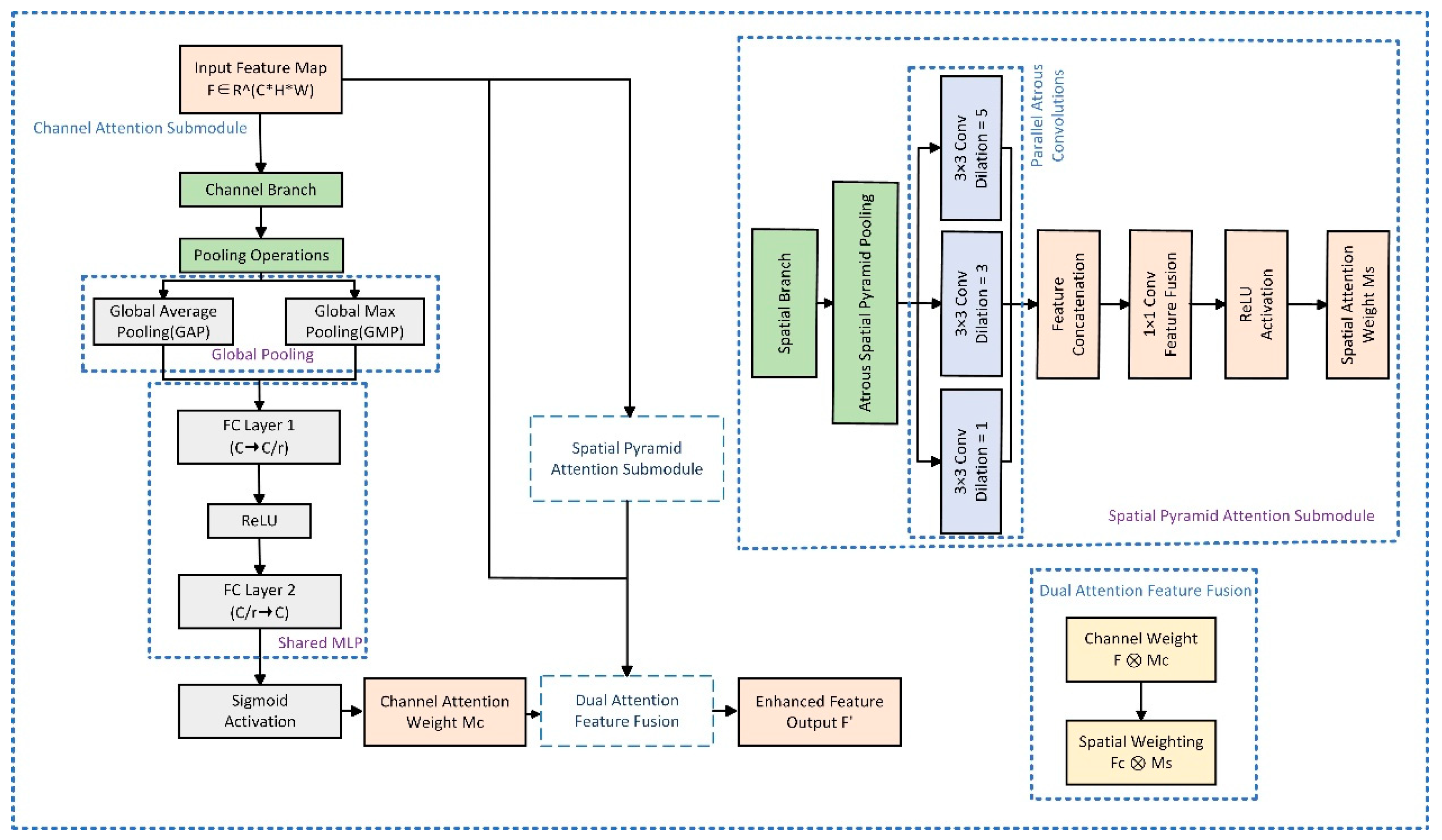
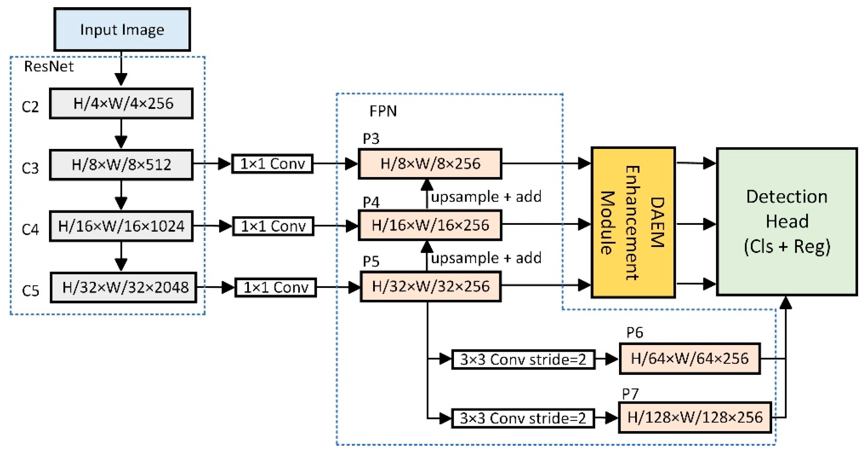
Along the three axes of where to fuse, how to enhance, and to what strength, we conduct an asymmetric exploration from shallow to deep. We first test two lightweight asymmetric prototypes. AsymmetricFPNv1 performs node level light reweighting and site specific adjustments, yielding marginal gains at near baseline compute. AsymmetricFPNv2 expands cross-level interactions and introduces stronger coupling; despite higher compute, mAP@[0.5:0.95] decreases and stability is insufficient. These results indicate that ad hoc, piecemeal changes are inadequate to coordinate strong semantic flames and weak contrast smoke. To systematically assess whether strong enhancement is necessary, we introduce a Dual Attention Enhancement Module (DAEM) at post-fusion sites and construct AsymmetricFPNv3. Figure 2 summarizes the structure of DAEM, which applies channel then spatial pyramid calibration. Figure 3 shows how this is attached at the post-fusion sites P3 to P5. Ablations reveal a complexity trap, parameters and compute increase notably, optimization becomes harder, and overall mAP@[0.5:0.95] declines. We therefore shift to a more targeted and lightweight post-fusion refinement strategy, laying the groundwork for the subsequent LEB and the final architecture.

In practice, DAEM is attached at the post-fusion nodes P3 to P5 to form the v3 architecture. This design verifies the hypothesis that strong enhancement can improve representation; however, under the unified protocol, the additional parameters and compute make optimization harder and reduce overall mAP@[0.5:0.95]. Accordingly, we pivot to a task-oriented lightweight post-fusion refinement to achieve a better balance between accuracy and efficiency.

Building on the observed complexity trap, we pivot to task-oriented lightweight post-fusion refinement and propose a Lightweight Enhancement Block (LEB), aiming to achieve generalizable feature recalibration at minimal compute and parameter cost. As shown in Figure 4, LEB uses depth-wise separable convolution as the basic operator [35] to sample spatial features at low cost, followed by a 1 × 1 pointwise convolution for channel mixing; it is paired with Group Normalization to maintain stability under small batch training [36], and a residual connection to preserve the identity mapping and gradient flow [33]. This minimal design follows an integrate-then-refine principle and serves as the atomic unit for subsequent choices of insertion site and strength, providing controllable gains in both accuracy and efficiency.

LEB formulation and cost. The block is defined as

$$Y=X+W_{PW}·SiLU\left(GN\right({DW}_{3\times 3}\left(X\right)\left)\right),$$

(4)

where X and Y are C × H × W feature maps, ${DW}_{3\times 3}$ is a depth-wise 3 × 3 convolution, GN is Group Normalization, SiLU is the activation, and $W_{PW}$ is a 1 × 1 pointwise convolution. The residual path stabilizes refinement with minimal overhead. For clarity, complexity counts include only convolutional terms:

$${FLOPs}_{DW}=H\times W\times C\times 3\times 3,{Params}_{DW}=C\times 3\times 3,$$

(5)

$${FLOPs}_{PW}=H\times W\times C\times C,{Params}_{PW}=C\times C,$$

(6)

Unless otherwise stated, FLOPs and parameters are counted by convolutional terms. For the LEB, the depth-wise 3 × 3 and the pointwise 1 × 1 terms are enumerated explicitly; bilinear up-sampling is counted separately. Following common practice, GroupNorm and activations are not included in FLOPs; at 640 × 640, their runtime overhead is small (estimated <1–2% per image). Under the unified setting on P3–P5, the 1 × 1 pointwise term contributes the dominant share and the depth-wise 3 × 3 contributes ~6–12%, consistent with Equations (5) and (6). We use Group Normalization with 32 groups by default on the P3–P5 feature channels; when the channel width C is smaller than 32, the number of groups is set to min (32, C) to keep each group non-trivial. SiLU is chosen as the activation in LEB because it provides smooth gradients and stable convergence under small-batch GN, while adding negligible runtime overhead compared with ReLU in our setting. Given the budget in Equations (5) and (6), we estimate that adding one extra LEB on P6 and P7 would increase the per-image FLOPs by less than 3% at 640 × 640; since our dataset contains relatively few ultra-small targets at those strides, we keep P6/P7 unchanged to avoid extra latency and preserve the near-baseline compute. We will provide a code path to optionally enable P6/P7 placement in future releases.

Cost interpretation and design implications. Equation (5) shows that the depth-wise 3 × 3 term scales linearly with C and is relatively cheap, whereas Equation (6) shows that the 1 × 1 pointwise term scales as H × W × C × C and therefore dominates the per-level cost. With a fixed channel width, compute grows primarily with spatial resolution. To keep GFLOPs near baseline, we use a single LEB per level, avoid stacking, and place it where multiscale context is already integrated, so the refinement is executed once per level rather than being re-aggregated by the top-down pathway. As reported, complexity counts include only the main convolutional terms and omit normalization and activation.

Informed by the cost analysis in Equations (5) and (6), we place exactly one LEB on P3 to P5 and keep the heads unchanged, which explains the near-baseline compute and the gains reported in

Table 1. Ablation under the unified protocol: accuracy and complexity. Training uses 4× RTX 2080 Ti with 640 × 640 input and a global batch size of 16; runtime is measured on a single RTX 2080 Ti with batch size 1, including warm up and NMS.

Model Configuration	mAP@[0.5:0.95]	mAP@0.5 (%)	Aps (%)	Params (M)	GFLOPs
Strong baseline	43.8	82.7	24.4	36.3	209.8
CIoU baseline	43.1	82.4	25.2	36.3	210.0
AsymFPNv1	43.4	83.1	24.1	36.9	209.8
AsymFPNv2	42.3	84.3	19.4	37.5	218.8
AsymFPNv3	42.8	85.4	26.6	38.2	251.6
AsymFPNv4	43.1	85.3	24.8	41.9	223.0
AsymFPNv5	44.0	85.5	25.3	36.5	211.0

Notes. APs denotes AP for small objects under the COCO scale definition. GFLOPs are computed for a single 640 × 640 forward pass using a FLOPs counter, including the FPN and heads on P3–P7, and excluding data loading, preprocessing, and NMS. All models are trained and evaluated under identical settings per Section 2.3: training on 4 GPUs with fixed optimizer, schedule, and seed; end-to-end FPS measured on a single GPU with warm up and NMS. Best values are in bold; significant digits follow the main text.

and Figure 6. To isolate the effect of placement, we compare two variants under identical settings: AsymmetricFPNv4 adopts a pre-fusion strategy that refines the lateral features ${\theta }_{\mathcal{l}}$ before FPN fusion, whereas AsymmetricFPNv5 adopts a post-fusion strategy that refines the fused features $P_{\mathcal{l}}$ after the top-down aggregation. Figure 5 presents the controlled comparison. Results in Section 3.1 consistently favor post-fusion, as leveraging the FPN’s multiscale context enables more targeted and efficient calibration on already integrated features, yielding a better accuracy–efficiency balance. We therefore adopt AsymmetricFPNv5 as the final model. For clarity, we now formalize the FPN fusion and make the two insertion options explicit; Equation (7) gives the top-down fusion with lateral connections, and Equation (8) instantiates the pre-fusion and post-fusion placements. A brief explanation of the symbols follows, after which we present Figure 5.

$$\begin{array}{c}{P}_5={\theta }_5\left(C_5\right),\\ P_{\mathcal{l}}={\theta }_{\mathcal{l}}\left(C_{\mathcal{l}}\right)+Up\left(P_{\mathcal{l}+1}\right),\mathcal{l}\in \left\{\mathrm{3,4}\right\}.\end{array}$$

(7)

We evaluate Equation (7) in a top-down order to obtain P5, P4, and P3. When used, a 3 × 3 smoothing convolution ${\varphi }_{\mathcal{l}}$(·) produces ${\tilde{P}}_{\mathcal{l}}$ from $P_{\mathcal{l}}$; otherwise $P_{\mathcal{l}}$ is left unchanged. These feature maps are then used in Equation (8) to instantiate the two placement options.

$$\begin{array}{c}{Z}_{\mathcal{l}}=LEB\left({\theta }_{\mathcal{l}}\right(C_{\mathcal{l}}\left)\right),\mathcal{l}\in \left\{\mathrm{3,4},5\right\};\\ Z_{\mathcal{l}}=LEB\left(P_{\mathcal{l}}\right),\mathcal{l}\in \left\{\mathrm{3,4},5\right\}.\end{array}$$

(8)

Equation (8) activates exactly one placement at a time: $Z_{\mathcal{l}}$ = LEB(${\theta }_{\mathcal{l}}$($C_{\mathcal{l}}$)) defines the pre-fusion variant, while $Z_{\mathcal{l}}$ = LEB($P_{\mathcal{l}}$) defines the post-fusion variant. The pre-fusion path refines level local features whose effect can be partially re blended by the subsequent top-down aggregation Up($P_{\mathcal{l}+1}$). In contrast, the post-fusion path refines features after multiscale context has been integrated, preserving high-frequency cues of flames and low-contrast contours of smoke. With an identical budget of one LEB at P3 to P5, this choice explains why the post-fusion design achieves higher mAP@[0.5:0.95] at near baseline compute in Section 3.1. Figure 5 visualizes the two topologies and the insertion sites used in our controlled comparison. Symbols follow Equations (7) and (8); ${\theta }_{\mathcal{l}}$ is a 1 × 1 lateral convolution, Up(·) is up-sampling, and ${\varphi }_{\mathcal{l}}$(·) is an optional 3 × 3 smoothing convolution. Figure 5 compares the two placement options under identical settings, each using one LEB at P3 to P5 with the heads unchanged. The pre-fusion variant refines the lateral features ${\theta }_{\mathcal{l}}$($C_{\mathcal{l}}$) before fusion, whose effect can be partially re blended by the subsequent top-down aggregation. The post-fusion variant refines $P_{\mathcal{l}}$ after multiscale context has been integrated, which better preserves high-frequency cues of flames and low-contrast smoke contours. With the same budget, post-fusion achieves higher mAP@[0.5:0.95] at near baseline compute in Section 3.1 and aligns with the qualitative evidence of fewer false positives in glare and sunset scenes.

This subsection moves from the symmetric FPN assumption to an asymmetric, site selective paradigm tailored to heterogeneous fire and smoke. Lightweight asymmetric attempts (v1, v2) yield limited or unstable gains, while heavy enhancement (v3 with DAEM) triggers a complexity trap. We therefore introduce the Lightweight Enhancement Block, formalize its mapping and cost, and conduct a placement study that favors post-fusion refinement. The final architecture places one LEB per level at P3 to P5 after fusion and immediately before the heads; P6 and P7 are produced from P5 via 3 × 3 stride 2 convolutions without LEB, and the heads run on P3 to P7. This design achieves higher accuracy at near baseline compute and improves parameter efficiency. Next, Section 2.3 details the experimental setup and the unified evaluation protocol used for all results.

2.3. Experimental Setup

2.3.1. Hardware and Software

To ensure fairness and repeatability, all experiments are run on a single hardware and software stack. Implementations use PyTorch v1.10.0 with CUDA 11.2 and cuDNN on Ubuntu 18.04 with Python 3.8. Training is conducted on four NVIDIA GeForce RTX 2080 Ti GPUs, while end-to-end throughput and latency are measured on a single RTX 2080 Ti with timing that includes warm up and NMS, consistent with Section 2.3.2. Unless otherwise noted, all RetinaNet based variants are trained end-to-end with the AdamW optimizer [37]. Because AdamW decouples weight decay from the gradient update, we fix the same optimizer and hyperparameters across variants to enable fair ablations.

We adopt a learning rate schedule of linear warm up followed by cosine annealing without restarts [38]. The initial and minimum learning rates are ${lr}_0$ = 1 × 10⁻⁴ and ${lr}_{min}$ = 1 × 10⁻⁶, with a warmup length $T_{warm}$ = 500 iterations. Formally,

$$lr(t)=\left\{\begin{array}{c}{lr}_0·{\displaystyle \frac{t}{T_{warm}}}, 0\le t<T_{warm}\\ {lr}_{min}+{\displaystyle \frac{{lr}_0-{lr}_{min}}{2}}(1+cos{\displaystyle \frac{\pi (t-T_{warm})}{T-T_{warm}}}),T_{warm}\le t\le T\end{array}\right.$$

(9)

where t is the iteration index and T is the total number of iterations. This design couples rapid early progress with monotonic annealing and yields stable convergence under the heterogeneous patterns of fire and smoke.

Training uses a global batch size of 16 for 100 epochs; with four GPUs, this corresponds to 4 samples per GPU. For comparability, external baselines are trained with their official recipes and then evaluated under the same environment and input resolution. Fixing the optimizer, the schedule, and the global batch size across all variants isolates the effects of the regression loss and the neck design, ensuring that the accuracy and efficiency differences reported in Section 3.1 can be attributed to architectural changes rather than optimization artifacts.

2.3.2. Reproducibility Details

We fix the random seed to 42 and propagate it to Python, NumPy, and PyTorch; we also set torch.cuda.manual_seed_all (42) and pass the seed to data workers via a worker_init_fn. Mixed precision is enabled with PyTorch AMP, using autocast for the forward pass and GradScaler for the backward pass. For cuDNN we set benchmark = True and deterministic = False; this favors speed and may introduce minor non bitwise differences, but results are statistically reproducible under our protocol. The data loader uses ${num}_{workers}$ = 8 and ${pin}_{memory}$ = True; training loaders are shuffled with ${drop}_{last}$ = True.

All inputs are letterboxed to 640 × 640 with aspect ratio preserved by padding; bounding boxes are rescaled accordingly. Unless otherwise noted, images are normalized by ImageNet means and standard deviations, and we use lightweight augmentation: random horizontal flip with probability 0.5 and random scale jitter in [0.8, 1.2]. For RetinaNet heads, the Focal Loss uses alpha = 0.25 and gamma = 2. Anchors use base sizes {32, 64, 128, 256, 512}, aspect ratios {1:2, 1:1, 2:1}, and scales {$2^0$, $2^{{\displaystyle \frac{1}{3}}}$, $2^{{\displaystyle \frac{2}{3}}}$}. Assignment uses IoU ≥ 0.5 for positives and IoU ≤ 0.4 for negatives, with anchors in between ignored. Inference uses score_threshold = 0.05, NMS IoU = 0.5, model.eval (), and torch.no_grad (). Exponential moving average (EMA) is not used.

Optimization uses AdamW with betas (0.9, 0.999) and weight decay 0.05. The learning rate schedule follows Equation (9): a 500-iteration linear warm up from ${lr}_0$ = 1 × 10⁻⁴, followed by cosine annealing without restarts down to ${lr}_{min}$ = 1 × 10⁻⁶. Floating point operations are reported for a single 640 × 640 forward pass using a FLOPs counter, including the FPN and heads on P3–P7, and excluding data loading, preprocessing, and NMS. Normalization and activation FLOPs are excluded; bilinear up-sampling is included separately. This convention is used consistently across all variants to enable budget-matched comparisons. End-to-end throughput is measured on a single RTX 2080 Ti with batch size 1 after 50 warm up and 200 timed iterations; torch.cuda.synchronize () is invoked before timing. The timed pipeline includes CPU side letterboxing and normalization, the model forward pass, and NMS/post-processing. Test time augmentation is not used.

2.4. Evaluation Metrics

We use a single, transparent set of metrics to assess accuracy, efficiency, and deploy ability. Accuracy is measured by the COCO-style mean average precision (mAP) [32], computed with pycocotools on 640 × 640 letterboxed inputs without test time augmentation. We report mAP@0.5, reflecting detection capability, and mAP@[0.5:0.95], emphasizing localization quality. Because early wildfire monitoring is safety-critical, we also report recall under the same inference thresholds.

To quantify accuracy per unit model size, we define a parameter efficiency ratio η as

$$\eta ={\displaystyle \frac{mAP@0.5}{Parameters\left(M\right)}},$$

(10)

where Parameters (M) denotes the number of trainable weights in millions. This ratio reads as mAP@0.5 points per million parameters and highlights compact designs when absolute accuracy is comparable. To avoid over-interpretation, η is always shown alongside absolute mAP and compute.

Efficiency and runtime are reported as follows. GFLOPs are measured for a single 640 × 640 forward pass using a FLOPs counter, including the FPN and heads on P3–P7, and excluding data loading, preprocessing, and NMS. End-to-end FPS is measured on a single RTX 2080 Ti with batch size 1 after 50 warm-up and 200 timed iterations; the timed pipeline includes CPU-side letterboxing and normalization, the model forward pass, and NMS/post-processing, with CUDA synchronization before timing. All models follow this unified inference and timing protocol unless otherwise stated.

3. Results

3.1. Ablation Study and Architectural Evolution

Under the unified protocol in Section 2.3, we ablate the key choices that lead from the baseline to AsymmetricFPNv5. Unless noted otherwise, the optimizer and schedule, 640 × 640 input, thresholds and timing, random seed, and data processing remain fixed to isolate architectural effects. We vary three factors. First, we replace Smooth L1 with CIoU to assess its impact on localization and small objects. Second, we explore the asymmetric pyramid evolution v1–v3, spanning from lightweight asymmetry to a heavy DAEM to probe enhancement strength and cross-level coupling. Finally, we study the placement of a single LEB per level, comparing pre-fusion in v4 that refines ${\theta }_{\mathcal{l}}$($C_{\mathcal{l}}$) with post-fusion in v5 that refines $P_{\mathcal{l}}$ under the same compute budget.

Table 1 reports mAP@[0.5:0.95], mAP@0.5, APs, parameter count, and GFLOPs for all variants. We highlight three references: the Strong baseline, the CIoU baseline, and the asymmetric pyramid variants. Taken together with Figure 6, the results show that early lightweight asymmetry (v1, v2) yields limited or unstable gains, whereas heavy enhancement (v3) triggers a complexity trap. With one LEB on P3 to P5, the post-fusion variant (v5) attains higher accuracy and parameter efficiency at near baseline compute.

Reading Table 1 yields four observations. First, replacing Smooth L1 with CIoU slightly lowers mAP@[0.5:0.95] while improving APs, consistent with tighter geometric supervision stabilizing small object regression. Second, lightweight asymmetric adjustments produce mixed outcomes: v1 nudges accuracy upward at essentially baseline compute, whereas v2 increases compute yet lowers mAP@[0.5:0.95], indicating that cross-level interactions must be designed with care. Third, uniformly attaching heavy dual attention raises compute to the highest level and reduces mAP@[0.5:0.95] despite a higher APs, revealing an unfavorable optimization capacity trade-off at this scale. Finally, concentrating one lightweight block per level at P3 to P5 after fusion delivers the top mAP@[0.5:0.95] = 44.0% with near baseline compute and a parameter count close to the baseline, outperforming the pre-fusion placement in both accuracy and efficiency.

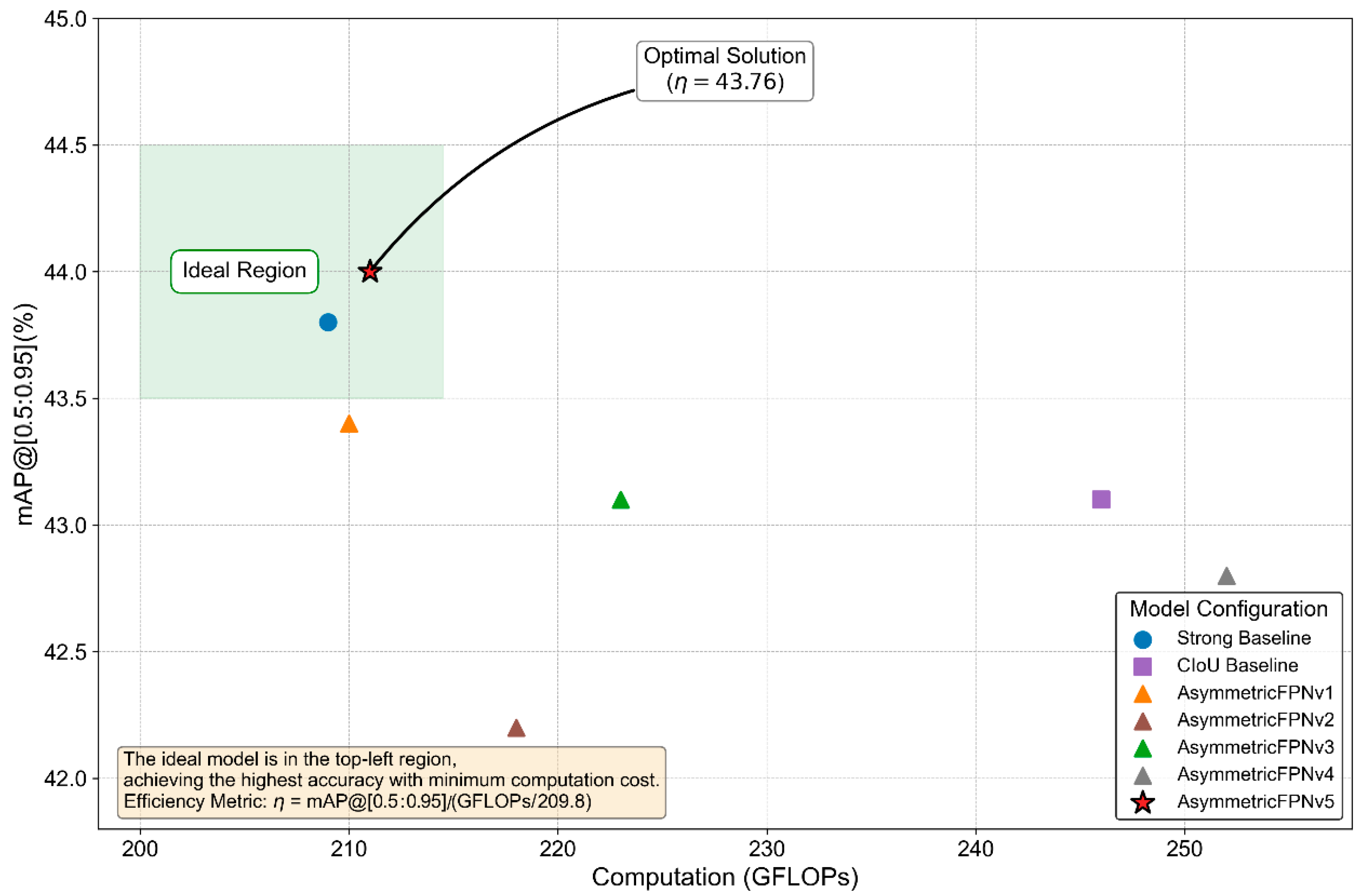
To visualize how accuracy scales with compute along this ablation path, Figure 6 plots mAP@[0.5:0.95] versus GFLOPs for all variants under the unified protocol. The preferred region is the upper left. The heavy dual attention design shifts rightward to the highest compute and slightly downward in accuracy, whereas the pre-fusion lightweight variant recovers accuracy with moderate compute. The post-fusion variant attains the highest mAP@[0.5:0.95] among all variants with only a small GFLOPs increase over the baseline. These trends are consistent with Table 1: localized post-fusion refinement at P3 to P5 is more beneficial than uniformly attaching heavy modules across pyramid levels.

From Table 1 and Figure 6, pre-fusion allocates capacity before lateral aggregation. Although it improves source level features, its effect is easily remixed by the subsequent top-down pathway, amplifying level specific bias; uniformly attaching heavy dual attention at all levels further raises compute and optimization difficulty, reducing localization accuracy in mAP@[0.5:0.95]. In contrast, post-fusion refines $P_{\mathcal{l}}$ after multiscale context has been integrated, letting the lightweight block exploit semantic and spatial cues jointly. With the same budget, placing one LEB per level at P3 to P5, P6 and P7 are derived from P5 by down-sampling and left without LEB, attains the best mAP@[0.5:0.95] in this subsection at near baseline compute and parameter count, and this surpasses the pre-fusion placement on both mAP@0.5 and APs. This is consistent with the cost analysis in Equations (5) and (6) and corroborates the evolution from the complexity trap of heavy enhancement to the stable gains of lightweight post-fusion refinement.

For fairness, all points in Figure 6 follow the unified protocol in Section 2.3: identical inputs and thresholds; GFLOPs are measured per single 640 × 640 forward pass including the pyramid and heads; end-to-end timing includes warm up and post-processing with CUDA synchronization; the random seed and shared hyperparameters are fixed. Under these conditions, the relative ordering remains stable across repeated runs, so the differences can be attributed to architectural choices rather than measurement noise. This evidence also explains why the final design matches the mAP@0.5 and recall of larger one stage baselines with fewer parameters: limited capacity is placed at key sites where multiscale context has already been aggregated, yielding more effective refinement at modest cost. Section 3.2 next provides visual comparisons in representative scenes, followed by Section 3.3, which benchmarks the method against mainstream detectors under the unified protocol.

3.2. Qualitative Analysis

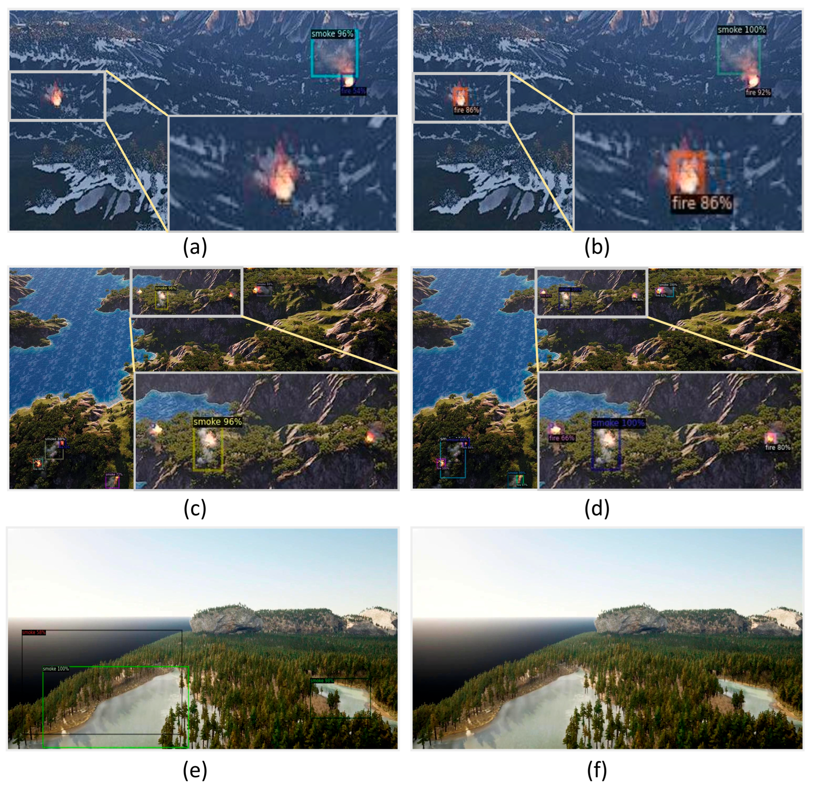
To complement the quantitative evidence in Section 3.1, we provide a controlled qualitative comparison that reveals how the design behaves under representative failure modes. We keep the inference protocol fixed and compare the Strong baseline with AsymmetricFPNv5 in a one-to-one manner on three scenes: distant small targets where high-frequency detail is easily diluted by symmetric fusion; multi-target scenes that stress contextual integration and recall; and complex backgrounds such as water glare and sunset that typically induce false positives. Figure 7 juxtaposes the detections of the two models, enabling a direct reading of accuracy and robustness gains that arise from localized post-fusion refinement at P3 to P5.

In the distant small target case (Figure 7a,b), the baseline becomes insensitive to weak fire signals because symmetric fusion dilutes high-frequency detail at higher resolutions; AsymmetricFPNv5 applies a single lightweight refinement per level at P3 to P5 after fusion, preserving and strengthening fine textures and recovering the missed target. In the multi-target scene (Figure 7c,d), the baseline tends to fire on the most salient instance only, whereas AsymmetricFPNv5 benefits from stronger context integration along the post-fusion path and achieves higher recall. In the complex background scene (Figure 7e,f), the baseline confuses water glare with smoke, revealing the limited discriminative power of a symmetric FPN under strong low level distractors, while AsymmetricFPNv5 decouples target attributes from background interference and improves precision, consistent with the design goal of localized post-fusion refinement. To substantiate this behavior, we visualize attention with Grad-CAM [39] on the same false positive scene as Figure 7e, revealing how the models allocate focus under the unified protocol (Figure 8).

Figure 8 shows fundamentally different attention patterns in the same complex scene. The baseline exhibits a strong and concentrated spurious activation over water glare, reflecting a decision process that relies on isolated low level cues and ignores scene context; AsymmetricFPNv5 markedly attenuates the activation on the same distractor and reallocates focus to target driven regions and boundaries. This aligns with our mechanism: localized refinement on $P_{\mathcal{l}}$ after multiscale integration, with one lightweight enhancement per level placed only at P3 to P5, corrects the attention drift induced by symmetric fusion and reduces false positives without a notable compute increase. Taken together with Figure 7, these qualitative results substantiate the quantitative gains reported in Section 3.1 and explain why post-fusion refinement improves discrimination and robustness. Next, Section 3.3 benchmarks the method against mainstream detectors under the unified protocol to quantify the overall benefits in accuracy, efficiency, and deployability. Under the unified thresholds, two dominant failure modes are observed. First, ultra-small distant fires can be missed when long-range high-frequency cues are diluted; the post-fusion refinement recovers part of these cases by preserving fine textures at P3–P5 (Figure 7a,b). Second, water-surface sun-glare induces false positives due to low-level appearance similarity to smoke; the proposed design suppresses these spurious activations by reallocating attention to target-driven regions and boundaries (Figure 7e,f and Figure 8). Residual errors mainly include thin, semi-transparent plumes in heavy haze and extremely small targets near the sensor limit. Scripts for per-scenario confusion counting will be provided in the companion repository upon acceptance.

3.3. Comparison with State-of-the-Art Models

Under a unified evaluation protocol, we benchmark AsymmetricFPNv5 against representative detectors, including the two stage Faster R-CNN and the single stage YOLO family (YOLOX and YOLOv8). To ensure fairness, all methods use official implementations and recommended hyperparameters, and follow the same settings as Section 2.3: 640 × 640 input, fixed thresholds and timing procedure, and no test time augmentation. We first compare accuracy (

Table 2. Accuracy comparison with mainstream detectors under the unified protocol.

Model Configuration	mAP@[0.5:0.95]	mAP@0.5 (%)	Recall (%)
Faster R-CNN	14.0	43.6	39.8
RetinaNet (R-50)	34.8	77.9	74.3
YOLOX-l	48.2	84.9	80.5
YOLOX-x	48.6	84.8	80.7
YOLOv5l	48.6	85.3	81.6
YOLOv5x	48.5	86.2	82.0
YOLOv8l	49.4	85.5	81.5
YOLOv8x	48.1	84.9	80.9
AsymmetricFPNv5	44.0	85.5	81.2

Notes. Metrics are computed with pycocotools on 640 × 640 letterboxed inputs without test-time augmentation; thresholds and timing follow Section 2.3. All models use official implementations and recommended hyperparameters under the same environment. Higher is better for all metrics.

), focusing on mAP@0.5 and recall with RetinaNet (R-50) as the in-framework reference; we then present model size and runtime efficiency in

Table 3. Model complexity and end-to-end speed under the unified protocol.

Model Configuration	Params (M)	GFLOPs	FPS	η	η@[0.5:0.95]
Faster R-CNN	41.5	246.3	30.28	1.05	0.34
RetinaNet (R-50)	37.9	246.0	34.45	2.06	0.92
YOLOX-l	54.2	155.6	62.68	1.57	0.89
YOLOX-x	99.1	281.9	35.36	0.86	0.49
YOLOv5l	46.1	107.7	77.83	1.85	1.05
YOLOv5x	86.1	203.8	42.51	1.00	0.56
YOLOv8l	43.6	164.8	59.36	1.96	1.13
YOLOv8x	68.1	257.4	38.94	1.25	0.71
AsymmetricFPNv5	36.5	211.0	26.10	2.34	1.21

Notes. Params (M) denotes trainable parameters in millions. GFLOPs are computed for a single 640 × 640 forward pass. FPS is measured end-to-end on a single RTX 2080 Ti with batch size 1 after warm up; the timed pipeline includes preprocessing and NMS. Parameter efficiency is defined as η = mAP@0.5/Params (M). The localization-aware efficiency is defined as η@[0.5:0.95] = mAP@[0.5:0.95]/Params (M).

to provide a complete view of the trade-off among performance, compute, and deployability.

Beyond accuracy, we compare model complexity and runtime efficiency. Under the same protocol as Section 2.3, Table 3 summarizes parameter count, GFLOPs, end-to-end FPS, and the parameter efficiency η defined as mAP@0.5/Params (M). Although the YOLO family typically leads in throughput, AsymmetricFPNv5 delivers 26.10 FPS on a single GPU, meeting real time requirements for early wildfire warning; more importantly, with 36.5 M parameters and near-baseline compute, it attains the highest η = 2.34, evidencing a light yet effective design. We next report the complexity and speed results in Table 3.

As shown in Table 3, AsymmetricFPNv5 attains the highest parameter efficiency η = 2.34 and also the highest localization-aware efficiency η@[0.5:0.95] = 1.21. This indicates that, with only 36.5 M parameters, our model delivers detection accuracy on par with YOLOv8l at 43.6 M, yielding the greatest performance per parameter and validating a light yet strong design. Such efficiency is crucial for deployment on edge platforms with constrained compute and energy, such as UAVs. In summary, the comparisons confirm that AsymmetricFPNv5 maintains SOTA tier-detection accuracy while achieving the best parameter efficiency, offering an attractive new balance among performance, efficiency, and deployment cost for wildfire detection.

4. Discussion

Accordingly, for forest fire detection, we revisit the information flow in FPN from the perspective of evaluation metrics and introduce node selection optimization to better balance accuracy, latency, and cost. Within the RetinaNet framework, we replace Smooth L1 with CIoU to enforce consistent modeling of overlap, center distance, and aspect ratio, thereby stabilizing regression for small objects. We further exploit the differences between flames and smoke in semantic strength and shape stability, where flames exhibit stronger semantics and relatively stable shapes, whereas smoke has low-contrast, fuzzy boundaries, and pronounced deformation. We break the symmetric treatment across FPN levels and, after feature fusion, apply lightweight level specific enhancement to different levels, forming an asymmetric feature pyramid. This design prevents over concentration on a single scale, reduces computation, and improves generalization. It maintains stable attention and reduces false positives under strong backgrounds such as water glare, sunset, and clouds, aiming for both low false alarm rates and high recall.

4.1. Practical Applicability and Deployment

The detector targets camera networks and UAV patrols where long-range small targets and glare or haze are frequent. We keep the standard RetinaNet heads and add one lightweight post-fusion refinement per level (P3–P5), so integration into existing pipelines requires minimal change.

Under the unified protocol we use score_threshold = 0.05 and NMS IoU = 0.5. In practice these values are site-tuned to trade-off miss rate and false alarms: higher thresholds suppress isolated glare-induced activations, while lower thresholds improve distant-small-target recall. Calibration is recommended on a small site-specific set containing hard negatives such as water-surface glare and sunset, together with representative positives. Timing includes CPU-side letterboxing and normalization, the model forward pass, and NMS with CUDA synchronization. With batch size 1 on a single RTX 2080 Ti, the measured end-to-end throughput is 26.10 FPS after warm-up, which satisfies real-time monitoring. The same protocol should be used for acceptance testing to avoid inconsistencies from excluding preprocessing or NMS. With 36.5M parameters and near-baseline GFLOPs, the model fits edge GPUs commonly used onboard UAVs or at towers. Memory footprint and latency are preserved because the heads are unchanged and only one lightweight refinement is applied per level. The model runs out-of-the-box with the standard RetinaNet data loader, anchor settings, and post-processing.

No re-training is required for site onboarding. Operators adjust score/NMS thresholds and, optionally, class-wise confidence scaling to meet local alert policies. When false alarms are dominated by glare, emphasize hard negatives during threshold sweeps; when long-range recall is critical, prefer a lower score threshold with slightly stricter NMS IoU. For video streams, a simple temporal persistence filter (for example, require at least two consecutive frames) further suppresses sporadic activations at negligible cost.

4.2. Attributing the Success of AsymmetricFPNv5 and the Path to an Efficiency Optimum

Our central finding is that task-oriented, asymmetric, lightweight post-fusion refinement achieves higher parameter efficiency for early wildfire detection than a symmetric FPN and several heavy state-of-the-art designs. The ablations in Section 3.1 form a coherent evidence chain: early lightweight asymmetry (v1, v2) yields limited or unstable gains; uniformly attaching a heavy dual-attention module across-levels (v3) inflates compute and degrades localization accuracy, constituting a complexity trap; under the same compute budget, placing exactly one lightweight block per level at P3–P5 after fusion (v5) delivers the best mAP@[0.5:0.95], outperforms the pre-fusion placement (v4) on both mAP@0.5 and APs, and keeps parameters and GFLOPs near the baseline.

Mechanistically, flames are strong-semantic, high-frequency, and edge-sharp, whereas smoke is low-contrast, diffuse, and weak-texture. Symmetric fusion tends to dilute high-frequency detail and class separability during top-down aggregation. In contrast, post-fusion refinement operates on Pℓ after multiscale context has been integrated, letting a lightweight block act exactly where semantic cues and spatial detail are jointly available—preserving flame boundaries while maintaining discernible smoke contours. Equation (4) shows that the LEB provides minimal residual refinement, and Equations (5) and (6) indicate that the dominant cost lies in the 1 × 1 pointwise term; therefore, once per level and only at P3–P5 controls complexity and avoids re-aggregation dilution. These behaviors align with the Grad-CAM visualizations in Section 3.2, which show more stable background suppression and tighter attention.

Overall, AsymmetricFPNv5 attains the same performance tier in mAP@0.5 and recall as larger one-stage baselines with fewer parameters and achieves the highest parameter efficiency η while providing practical end-to-end throughput. Rather than escalating a module-stacking arms race, this suggests a reusable architectural principle: perform the right lightweight refinement at the right post-fusion sites to balance accuracy, efficiency, and deployment cost.

4.3. Comparison and Reflection on SOTA Models Rebalancing Accuracy Speed and Efficiency

As shown in Section 3.3, under the unified protocol, AsymmetricFPNv5 reaches the same performance tier as YOLOv8l on mAP@0.5 and recall, while using fewer parameters (36.5 M vs. 43.6 M). Its end-to-end throughput is slightly lower but reaches 26.10 FPS, which satisfies real time warning requirements. Together with Table 3, this yields the highest parameter efficiency in this study (η = 2.34) at near baseline compute, indicating higher accuracy per unit model size without sacrificing core detection capability. On edge platforms such as UAVs, model size and compute constrain memory footprint and energy, and thus sustained operation; efficiency and deployability should be considered alongside accuracy. We therefore advocate moving from a two-dimensional objective of mAP and FPS to a three-dimensional co optimization of mAP, FPS, and parameter efficiency η. The evidence suggests that task-oriented lightweight refinement at key post-fusion sites provides a practical route to balance accuracy, speed, and efficiency. In relation to lightweight necks such as PAN-Lite and BiFPN-Lite, prior reports target cross-level aggregation with depth-wise/separable convolutions and learned fusion. Our design keeps the RetinaNet heads unchanged and applies a single post-fusion refinement per level on P3–P5, which minimizes integration cost while delivering the highest η and η@[0.5:0.95] at near-baseline compute under our unified protocol. A budget-matched reproduction of PAN-Lite/BiFPN-Lite within the same protocol is planned; upon acceptance, we will release code paths for neck swapping and report results in the companion repository.

4.4. Limitations and Future Work

Despite the encouraging results, several limitations remain. First, although our composite dataset was carefully merged and deduplicated, its scene diversity is still limited compared with large general purpose sets; we will expand to extreme weather and night scenes to further stress robustness and cross domain generalization. Second, our innovations focus on the FPN neck while the backbone remains ResNet 50; combining AsymmetricFPN with more advanced and efficient backbones, such as Swin Transformer or ConvNeXt, is expected to bring additional gains [40]. Third, the parameter efficiency η is an aggregate indicator and does not fully capture deployment cost; we plan to adopt a more granular efficiency model that reports measured power, latency, memory usage, and throughput, and to include an additional efficiency variant based on mAP@[0.5:0.95]. We will also extend evaluations to diverse edge hardware and release unified measurement scripts to support reproducible and green deployment. While Section 3.2 already contrasts representative failure modes (distant tiny targets and water-glare scenes) under unified thresholds, we did not include a fine-grained domain-wise table in the main paper because reliable per-image scene metadata is not consistently available and some groups remain small, which may invite over-interpretation. We will release scripts for domain-wise evaluation (e.g., source: synthetic/real; scene: glare/non-glare; lighting) together with templates for site-specific grouping in the companion repository upon acceptance. We presently report end-to-end latency/FPS on an RTX 2080 Ti under the unified protocol. Embedded measurements on Jetson Orin/Xavier and ARM CPU at 640 × 640 with the identical pipeline (including preprocessing and NMS) are planned. Upon acceptance, we will provide a hardware-agnostic timing script and environment (Docker/conda) and report measured latency/FPS, peak memory, and power on embedded devices in the companion repository. We currently report point estimates under the unified protocol. To quantify statistical variability, we will provide scripts to compute 95% confidence intervals via image-level bootstrap on the test set and to run ≥3 seeds, together with per-run logs and the v5 checkpoint, in the companion repository upon acceptance. The unified settings (fixed thresholds and timing) are kept to ensure that relative ordering is not confounded by protocol changes.

5. Conclusions

To reconcile accuracy and deployability for early wildfire monitoring, we propose AsymmetricFPNv5, an asymmetric feature pyramid centered on parameter efficiency. Rather than a symmetric FPN or heavy module stacking, the method performs lightweight post-fusion refinement at key sites where multiscale context is already integrated, placing a single LEB per level at P3–P5 to calibrate heterogeneous fire and smoke features with minimal compute. Extensive ablations and comparisons confirm the effectiveness of this paradigm. Under our deduplicated composite dataset and unified protocol, AsymmetricFPNv5 achieves mAP@0.5 of 85.5% and recall of 81.2%, and attains the highest parameter efficiency with η = 2.34; its end-to-end throughput meets real time warning requirements.

Overall, AsymmetricFPNv5 offers a light-yet-effective solution for wildfire detection and demonstrates that task-oriented, efficiency-driven architecture—performing the right lightweight refinement at the right post-fusion sites—can break the performance—cost bottleneck and yield a better balance among accuracy, efficiency, and deployment cost. Future work will pair the method with stronger and more efficient backbones, extend to extreme and night scenes, and develop a more comprehensive efficiency evaluation including measured power, latency, memory, and throughput to enable greener deployment on diverse edge hardware.

References

1. Food and Agriculture Organization of the United Nations. Global Forest Resources Assessment 2020: Key Findings; Food and Agriculture Organization of the United Nations: Rome, Italy, 2020; ISBN 978-92-5-132581-0. [Google Scholar] [CrossRef]
2. Jones, M.W.; Abatzoglou, J.T.; Veraverbeke, S.; Andela, N.; Lasslop, G.; Forkel, M.; Smith, A.J.P.; Burton, C.; Betts, R.A.; van der Werf, G.R.; et al. Global and Regional Trends and Drivers of Fire Under Climate Change. Rev. Geophys. 2022, 60, e2020RG000726. [Google Scholar] [CrossRef]
3. Mohapatra, A.; Trinh, T. Early Wildfire Detection Technologies in Practice—A Review. Sustainability 2022, 14, 12270. [Google Scholar] [CrossRef]
4. Barmpoutis, P.; Papaioannou, P.; Dimitropoulos, K.; Grammalidis, N. A Review on Early Forest Fire Detection Systems Using Optical Remote Sensing. Sensors 2020, 20, 6442. [Google Scholar] [CrossRef] [PubMed]
5. Chan, C.C.; Alvi, S.A.; Zhou, X.; Durrani, S.; Wilson, N.; Yebra, M. A Survey on IoT Ground Sensing Systems for Early Wildfire Detection: Technologies, Challenges, and Opportunities. IEEE Access 2024, 12, 172785–172819. [Google Scholar] [CrossRef]
6. Zhu, W.; Niu, S.; Yue, J.; Zhou, Y. Multiscale wildfire and smoke detection in complex drone forest environments based on YOLOv8. Sci. Rep. 2025, 15, 2399. [Google Scholar] [CrossRef] [PubMed]
7. Ramos, L.; Casas, E.; Bendek, E.; Romero, C.; Rivas-Echeverría, F. Hyperparameter optimization of YOLOv8 for smoke and wildfire detection: Implications for agricultural and environmental safety. Artif. Intell. Agric. 2024, 12, 109–126. [Google Scholar] [CrossRef]
8. Huang, J.; Zhou, J.; Yang, H.; Liu, Y.; Liu, H. A Small-Target Forest Fire Smoke Detection Model Based on Deformable Transformer for End-to-End Object Detection. Forests 2023, 14, 162. [Google Scholar] [CrossRef]
9. Park, G.; Lee, Y. Wildfire Smoke Detection Enhanced by Image Augmentation with StyleGAN2-ADA for YOLOv8 and RT-DETR Models. Fire 2024, 7, 369. [Google Scholar] [CrossRef]
10. Bakirci, M.; Bayraktar, I. Harnessing UAV Technology and YOLOv9 Algorithm for Real-Time Forest Fire Detection. In Proceedings of the 2024 International Russian Automation Conference (RusAutoCon), Sochi, Russian Federation, 8–14 September 2024; IEEE: Piscataway, NJ, USA, 2024. [Google Scholar] [CrossRef]
11. Huang, X.; Xie, W.; Zhang, Q.; Lan, Y.; Heng, H.; Xiong, J. A Lightweight Wildfire Detection Method for Transmission Line Perimeters. Electronics 2024, 13, 3170. [Google Scholar] [CrossRef]
12. Gain, M.; Raha, A.D.; Biswas, B.; Bairagi, A.K.; Adhikary, A.; Debnath, R. LEO Satellite Oriented Wildfire Detection Model Using Deep Neural Networks: A Transfer Learning Based Approach. In Proceedings of the 2024 6th International Conference on Electrical Engineering and Information & Communication Technology (ICEEICT), Dhaka, Bangladesh, 2–4 May 2024; IEEE: Piscataway, NJ, USA, 2024; pp. 214–219. [Google Scholar] [CrossRef]
13. Shees, A.; Ansari, M.S.; Varshney, A.; Asghar, M.N.; Kanwal, N. FireNet-v2: Improved Lightweight Fire Detection Model for Real-Time IoT Applications. Procedia Comput. Sci. 2023, 218, 2233–2242. [Google Scholar] [CrossRef]
14. Li, J.; Tang, H.; Li, X.; Dou, H.; Li, R. LEF-YOLO: A lightweight method for intelligent detection of four extreme wildfires based on the YOLO framework. Int. J. Wildland Fire 2023, 33, WF23044. [Google Scholar] [CrossRef]
15. Ramadan, M.N.A.; Basmaji, T.; Gad, A.; Hamdan, H.; Akgün, B.T.; Ali, M.A.H.; Alkhedher, M.; Ghazal, M. Towards Early Forest Fire Detection and Prevention Using AI-Powered Drones and the IoT. Internet Things 2024, 27, 101248. [Google Scholar] [CrossRef]
16. Giannakidou, S.; Rodoglou-Grammatikis, P.; Lagkas, T.; Argyriou, V.; Goudos, S.; Markakis, E.K.; Sarigiannidis, P. Leveraging the Power of Internet of Things and Artificial Intelligence in Forest Fire Prevention, Detection, and Restoration: A Comprehensive Survey. Internet Things 2024, 26, 101171. [Google Scholar] [CrossRef]
17. Lin, T.-Y.; Goyal, P.; Girshick, R.; He, K.; Dollár, P. Focal Loss for Dense Object Detection. In Proceedings of the 2017 IEEE International Conference on Computer Vision (ICCV), Venice, Italy, 22–29 October 2017; IEEE: Piscataway, NJ, USA, 2017; pp. 2999–3007. [Google Scholar] [CrossRef]
18. Lin, T.-Y.; Dollár, P.; Girshick, R.; He, K.; Hariharan, B.; Belongie, S. Feature Pyramid Networks for Object Detection. In Proceedings of the 2017 IEEE Conference on Computer Vision and Pattern Recognition (CVPR), Honolulu, HI, USA, 21–26 July 2017; IEEE: Piscataway, NJ, USA, 2017; pp. 936–944. [Google Scholar] [CrossRef]
19. Tan, M.; Pang, R.; Le, Q.V. EfficientDet: Scalable and Efficient Object Detection. In Proceedings of the 2020 IEEE/CVF Conference on Computer Vision and Pattern Recognition (CVPR), Seattle, WA, USA, 13–19 June 2020; IEEE: Piscataway, NJ, USA, 2020; pp. 10778–10787. [Google Scholar] [CrossRef]
20. Hu, M.; Li, Y.; Fang, L.; Wang, S. A2-FPN: Attention Aggregation based Feature Pyramid Network for Instance Segmentation. In Proceedings of the 2021 IEEE/CVF Conference on Computer Vision and Pattern Recognition (CVPR), Nashville, TN, USA, 20–25 June 2021; IEEE: Piscataway, NJ, USA, 2021; pp. 15338–15347. [Google Scholar] [CrossRef]
21. Zhang, K.; Li, Z.; Hu, H.; Li, B.; Tan, W.; Lu, H.; Xiao, J.; Ren, Y.; Pu, S. Dynamic Feature Pyramid Networks for Detection. In Proceedings of the 2022 IEEE International Conference on Multimedia and Expo (ICME), Taipei, Taiwan, 18–22 July 2022; IEEE: Piscataway, NJ, USA, 2022. [Google Scholar] [CrossRef]
22. Jin, M.; Li, H. Feature-Aligned Feature Pyramid Network and Center-Assisted Anchor Matching for Small Face Detection. In Proceedings of the 2023 4th International Conference on Big Data, Artificial Intelligence and Internet of Things Engineering (ICBAIE), Hangzhou, China, 25–27 August 2023; IEEE: Piscataway, NJ, USA, 2023; pp. 198–204. [Google Scholar] [CrossRef]
23. Cazzato, D.; Cimarelli, C.; Sanchez-Lopez, J.L.; Voos, H.; Leo, M. A Survey of Computer Vision Methods for 2D Object Detection from Unmanned Aerial Vehicles. J. Imaging 2020, 6, 78. [Google Scholar] [CrossRef] [PubMed]
24. Ramos, L.; Casas, E.; Bendek, E.; Romero, C.; Rivas-Echeverría, F. Computer vision for wildfire detection: A critical brief review. Multimed. Tools Appl. 2024, 83, 83427–83470. [Google Scholar] [CrossRef]
25. Allison, R.S.; Johnston, J.M.; Craig, G.; Jennings, S. Airborne Optical and Thermal Remote Sensing for Wildfire Detection and Monitoring. Sensors 2016, 16, 1310. [Google Scholar] [CrossRef] [PubMed]
26. Bhatt, D.; Patel, C.; Talsania, H.; Patel, J.; Vaghela, R.; Pandya, S.; Modi, K.; Ghayvat, H. CNN Variants for Computer Vision: History, Architecture, Application, Challenges and Future Scope. Electronics 2021, 10, 2470. [Google Scholar] [CrossRef]
27. Liu, Y.; Sun, P.; Wergeles, N.; Shang, Y. A survey and performance evaluation of deep learning methods for small object detection. Expert Syst. Appl. 2021, 172, 114602. [Google Scholar] [CrossRef]
28. Ghali, R.; Akhloufi, M.A. Deep Learning Approaches for Wildland Fires Using Satellite Remote Sensing Data: Detection, Mapping, and Prediction. Fire 2023, 6, 192. [Google Scholar] [CrossRef]
29. Yunnan University. Synthetic Fire-Smoke. Roboflow Universe. 2023. Available online: https://universe.roboflow.com/yunnan-university/synthetic-fire-smoke (accessed on 6 March 2023).
30. Wildfire-Q3RM1. Wildfire. Roboflow Universe. 2024. Available online: https://universe.roboflow.com/wildfire-q3rm1/wildfire-ajbuc (accessed on 4 December 2024).
31. Dubey, S.R.; Singh, S.K.; Chu, W.-T. Vision Transformer Hashing for Image Retrieval. In Proceedings of the 2022 IEEE International Conference on Multimedia and Expo (ICME), Taipei, Taiwan, 18–22 July 2022; IEEE: Piscataway, NJ, USA, 2022. [Google Scholar] [CrossRef]
32. Lin, T.-Y.; Maire, M.; Belongie, S.; Hays, J.; Perona, P.; Ramanan, D.; Dollár, P.; Zitnick, C.L. Microsoft COCO: Common Objects in Context. In Lecture Notes in Computer Science; Springer: Cham, Switzerland, 2014; Volume 8693, pp. 740–755. [Google Scholar] [CrossRef]
33. He, K.; Zhang, X.; Ren, S.; Sun, J. Deep Residual Learning for Image Recognition. In Proceedings of the 2016 IEEE Conference on Computer Vision and Pattern Recognition (CVPR), Las Vegas, NV, USA, 27–30 June 2016; IEEE: Piscataway, NJ, USA, 2016; pp. 770–778. [Google Scholar] [CrossRef]
34. Zheng, Z.; Wang, P.; Liu, W.; Li, J.; Ye, R.; Ren, D. Distance-IoU Loss: Faster and Better Learning for Bounding Box Regression. In Proceedings of the AAAI Conference on Artificial Intelligence, New York, NY, USA, 7–12 February 2020; AAAI Press: Palo Alto, CA, USA, 2020; pp. 12993–13000. [Google Scholar] [CrossRef]
35. Zhao, T.; Xie, Y.; Wang, Y.; Cheng, J.; Guo, X.; Hu, B. A Survey of Deep Learning on Mobile Devices: Applications, Optimizations, Challenges, and Research Opportunities. Proc. IEEE 2022, 110, 334–354. [Google Scholar] [CrossRef]
36. Wu, Y.; He, K. Group Normalization. In Computer Vision—ECCV 2018. Lecture Notes in Computer Science; Ferrari, V., Hebert, M., Sminchisescu, C., Weiss, Y., Eds.; Springer: Cham, Switzerland, 2018; Volume 11217, pp. 3–19. [Google Scholar] [CrossRef]
37. Loshchilov, I.; Hutter, F. Decoupled Weight Decay Regularization. In Proceedings of the 7th International Conference on Learning Representations (ICLR), New Orleans, LA, USA, 6–9 May 2019; OpenReview.net: Alameda, CA, USA, 2019. [Google Scholar]
38. Loshchilov, I.; Hutter, F. SGDR: Stochastic Gradient Descent with Warm Restarts. In Proceedings of the 5th International Conference on Learning Representations (ICLR), Toulon, France, 24–26 April 2017; OpenReview.net: Alameda, CA, USA, 2017. [Google Scholar]
39. Selvaraju, R.R.; Cogswell, M.; Das, A.; Vedantam, R.; Parikh, D.; Batra, D. Grad-CAM: Visual Explanations from Deep Networks via Gradient-based Localization. In Proceedings of the 2017 IEEE International Conference on Computer Vision (ICCV), Venice, Italy, 22–29 October 2017; IEEE: Piscataway, NJ, USA, 2017; pp. 618–626. [Google Scholar] [CrossRef]
40. Liu, Z.; Mao, H.; Wu, C.-Y.; Feichtenhofer, C.; Darrell, T.; Xie, S. A ConvNet for the 2020s. In Proceedings of the 2022 IEEE/CVF Conference on Computer Vision and Pattern Recognition (CVPR), New Orleans, LA, USA, 18–24 June 2022; IEEE: Piscataway, NJ, USA, 2022; pp. 11966–11976. [Google Scholar] [CrossRef]
Figure 1. Challenging samples in the composite wildfire dataset (examples sourced from Roboflow Universe datasets synthetic fire smoke [29] and Wildfire [30]). (a) Distant tiny fire spots occupying only a few pixels; (b) multiple distant small targets coexisting; (c) specular reflections from water bodies or wetlands, with colors and brightness similar to firelight.
Applsci 15 12086 g001
Figure 2. Dual Attention Enhancement Module (DAEM). The module consists of a channel attention submodule and a spatial pyramid attention submodule. The channel branch applies global average pooling and global max pooling, followed by a shared MLP and a sigmoid, to produce channel weights Mc. The spatial branch aggregates three parallel 3 × 3 dilated convolutions with dilation rates 1, 3, and 5, followed by a 1 × 1 convolution, ReLU, and a sigmoid, to produce spatial weights Ms. The two weights are applied sequentially to the input feature map for adaptive recalibration, yielding the enhanced output F′.
Applsci 15 12086 g002
Figure 3. Overall architecture of AsymmetricFPNv3. DAEM is attached to the FPN post-fusion nodes P3–P5. P6 and P7 are generated from P5 by consecutive 3 × 3 convolutions with stride 2. Standard RetinaNet heads perform classification and regression on all pyramid levels P3–P7.
Applsci 15 12086 g003
Figure 4. Lightweight Enhancement Block (LEB). Composed of a 3 × 3 depth-wise convolution, Group Normalization, ReLU, a 1 × 1 pointwise convolution, and Group Normalization, with a residual skip connection and a final ReLU. This provides stable feature refinement at minimal compute.
Applsci 15 12086 g004
Figure 5. Placement study of the LEB. Pre-fusion in AsymmetricFPNv4: the LEB refines backbone features C3–C5 before lateral fusion, followed by the lateral path and the top-down pathway to produce P3–P7. Post-fusion in AsymmetricFPNv5: the LEB refines fused features P 3 r a w P 5 r a w after the top-down aggregation; the heads operate on P3–P7. Both variants place exactly one LEB at P3–P5 with all other settings identical, differing only in the ins[ertion site. Under the same budget, post-fusion achieves a better balance between accuracy and efficiency. Symbols follow Equations (7) and (8).
Applsci 15 12086 g005
Figure 6. Accuracy–compute trade-off under the unified protocol. Vertical: mAP@[0.5:0.95]; Horizontal: GFLOPs per 640 × 640 forward pass. Points: Strong baseline, CIoU baseline, and AsymmetricFPNv1–v5. The star marks the post-fusion variant v5, which achieves the highest mAP@[0.5:0.95] at near baseline compute; the upper-left region is preferred. Results are point estimates under the unified protocol; the relative ordering was consistent across repeated runs. 95% confidence intervals based on image-level bootstrap will be released in the companion repository.
Applsci 15 12086 g006
Figure 7. Qualitative comparisons under representative challenging scenes. Left: baseline; right: AsymmetricFPNv5. Panels (a,b) show distant small targets (zoomed-in crops are provided beneath each frame at ~×2.5 for readability). Because the targets are long-range, per-box labels may appear small at the journal layout size; the detections should be read from the colored boxes and the zoomed-in crops. Panels (c,d) show multi-target scenes where stronger context integration leads to higher recall. Panels (e,f) show complex backgrounds; the baseline confuses glare with smoke, whereas AsymmetricFPNv5 suppresses the distractor and improves precision. A high-resolution version of this figure is included in the submission files.
Applsci 15 12086 g007
Figure 8. Grad-CAM visualization for a complex background scene. Warmer colors indicate stronger activation; heatmaps are overlaid on the RGB image. (a) Input image. (b) Strong baseline: a concentrated spurious activation appears over the water-glare region, indicating reliance on low-level cues and weak contextual reasoning. (c) AsymmetricFPNv5: activation on the same distractor is markedly attenuated by asymmetric post-fusion refinement, enabling robust background suppression. Grad-CAM is computed on the last convolution in P5 with per-map min–max normalization before overlay; masking the top-activated regions flips the baseline decision in (b), but not v5 in (c), consistent with more context-aware focus after post-fusion refinement.
Applsci 15 12086 g008