AI-Enhanced Nonlinear Predictive Control for Smart Greenhouses: A Performance Comparison of Forecast and Warm-Start Strategies

Abstract

Accurate, energy-efficient climate regulation is crucial for scaling smart greenhouse production. While nonlinear model predictive control (NMPC) can co-optimize yield and resource use, its efficacy hinges on short-range weather information and real-time solver feasibility. This paper investigates the performance of advanced NMPC strategies for smart greenhouse climate control, with particular emphasis on the roles of AI-driven disturbance prediction and warm-start initialization for real-time optimization. Six controller configurations, including feedback-only, LSTM-based forecast, and ideal disturbance models, each with and without warm-start, were tested in a 40-day simulation of a lettuce smart greenhouse. Performance metrics included final biomass, constraint violations, resource costs, profit, and solver time. Results show that feedback-only controllers maximize yield and profit, incurring higher CO₂ costs but lower heating costs, alongside greater constraint violations compared to the predictive strategies. Predictive and ideal disturbance-aware controllers effectively reduce resource consumption and improve constraint compliance at the expense of lower yields. Importantly, warm-start initialization significantly accelerates computation without affecting control quality. The study also demonstrates that penalty parameters, rather than economic weight settings, predominantly determine aggregate constraint violation. The findings provide actionable insights for designing and deploying NMPC-based greenhouse controllers, highlighting the importance of warm-start techniques and the trade-offs between productivity, resource efficiency, and environmental compliance.

1. Introduction

Smart greenhouse agriculture plays an increasingly critical role in addressing global challenges such as food security, climate change, and sustainable development. These systems integrate automation, IoT technologies, and AI-driven control strategies to enable year-round, resource-efficient crop production. To achieve precise climate regulation in smart greenhouses, advanced control techniques have become essential, allowing growers to optimize yield and quality while minimizing energy and CO₂ consumption.

NMPC has emerged as a leading solution for greenhouse climate management, thanks to its capacity to handle nonlinear system dynamics, operational constraints, and multi-objective optimization [1,2,3]. Nevertheless, the effectiveness of NMPC relies heavily on the accurate prediction of environmental disturbances and the computational efficiency required for real-time implementation.

Recent advances in artificial intelligence and machine learning—especially deep neural networks such as Long Short-Term Memory (LSTM)—have enabled more accurate, data-driven forecasting of environmental variables [4,5]. Integrating such forecasts into NMPC frameworks offers the potential to anticipate and proactively mitigate external disturbances, improving both climate regulation and resource efficiency. However, most prior studies focus on single-variable prediction, and few have assessed the impact of multi-variable, AI-based forecasts on NMPC performance. In parallel, real-time NMPC is often hindered by the computational burden of repeatedly solving large-scale, constrained nonlinear optimization problems. Warm-start techniques, which leverage previous solutions to accelerate convergence, have shown significant promise in other application domains [6], but their practical impact in greenhouse NMPC—especially when coupled with advanced disturbance prediction—remains largely unexplored.

While progress has been made, there is still no systematic study that jointly evaluates the control and computational performance of NMPC under different disturbance forecasting strategies. To address these limitations, this study proposes an AI-enhanced NMPC framework in which a single multi-output LSTM network is trained to jointly forecast all major external disturbances—outdoor temperature, humidity, CO₂ concentration, and solar radiation—relevant to greenhouse climate control. By capturing temporal dependencies and nonlinear relationships among these variables, the LSTM model delivers comprehensive, realistic forecasts for proactive climate regulation. Furthermore, to provide a thorough and fair assessment, this work conducts a unified comparative study of three NMPC configurations: (1) feedback-only NMPC, assuming constant disturbances; (2) LSTM-based predictive disturbance NMPC, utilizing joint multi-variable AI-based disturbance prediction; and (3) ideal predictive disturbance NMPC, using true future disturbance profiles as an upper-bound benchmark. The practical value of warm-start optimization is also systematically investigated across all configurations. Utilizing a detailed lettuce greenhouse model [7] and extensive 40-day simulations, the effectiveness of feedback-only, predictive, and ideal preview controllers—with and without warm-start—is rigorously assessed using comprehensive key performance indicators (KPIs) such as final biomass yield, setpoint adherence, resource consumption, net profit, and solver computation time.

The findings of this research are expected to provide valuable, actionable insights for both researchers in control engineering and agricultural systems, as well as practitioners seeking to implement advanced AI-enabled control solutions for optimal greenhouse environmental management. The remainder of this paper is organized as follows: Section 2 reviews related literature. Section 3 details the greenhouse model. Section 4 describes the NMPC formulation, controller variants, and performance metrics. Section 5 outlines the simulation setup. Section 6 presents and discusses the results, and Section 7 concludes the paper.

2. Related Work

This section reviews relevant literature to contextualize the present study. Key areas explored include NMPC strategies for greenhouses, AI-based disturbance prediction, and warm-start techniques for computational efficiency in smart agricultural applications. The review culminates by identifying current research gaps, thereby framing the contributions of this study.

2.1. NMPC Strategies for Greenhouse Climate Control

The optimal control of greenhouse climate has a long history, with foundational work by van Henten framing greenhouse climate regulation as an open-loop optimal control problem aimed at maximizing net revenue [7]. Subsequent sensitivity analyses by van Henten also highlighted that uncertainties in humidity and radiation typically lead to the largest profit losses [8]. Time-scale decomposition of the optimal control problem has also been explored [9]. However, open-loop trajectories are not feasible for autonomous operation in dynamic environments, as they cannot correct for actual disturbances.

NMPC has emerged as an advanced closed-loop solution, offering distinct advantages for handling the complex nonlinear dynamics and operational constraints of horticultural systems [1,2]. NMPC has been applied to diverse objectives, such as reducing energy and water consumption [10], improving temperature control and energy utilization [11], and enabling smart energy management in plant factories [12]. Other notable applications include NMPC based on Volterra series models for temperature regulation [13].

To address system uncertainties, more advanced NMPC formulations have been proposed, including multi-scenario MPC considering market price uncertainty [3] [García-Mañas et al.], robust MPC [14], and chance-constrained stochastic MPC [15]. Concepts like the advanced-step NMPC controller have also been explored [16]. In parallel, the integration of data-driven and AI-based methods—such as reinforcement learning (RL) [17,18] and deep neural networks [19]—has received increasing attention, aiming to enhance adaptability and performance. A recent comprehensive comparison between RL and NMPC on lettuce greenhouse climate control found that while RL can offer adaptability and lower computational demands, NMPC retains superior constraint handling and economic performance under certain scenarios [20]. While NMPC provides a robust framework, its real-world performance still heavily relies on effective disturbance handling and the integration of predictive intelligence of future uncertainties.

2.2. Approaches to Disturbance Handling and Prediction in Greenhouse Control

In greenhouse NMPC, disturbance management can be approached either reactively (feedback-only) or proactively (predictive). While traditional NMPC often relies on current disturbance measurements (feedback-only), incorporating multi-step forecasts from AI models enables proactive adaptation and can significantly enhance control performance. The importance of weather forecast horizons has been investigated, for instance, in Jansen’s work, which, although RL-focused, highlights the impact of forecast horizons [21]. Kuijpers et al. have modeled weather forecast errors and analyzed their impact on automated greenhouse climate control systems [22].

ML has demonstrated significant advancements in general weather forecasting, as indicated in recent surveys [5,23]. For specific greenhouse applications, Esparza-Gómez et al. successfully applied a Recurrent Neural Network (RNN) with an LSTM model for temperature prediction, further illustrating the promise of ML for microclimate forecasting in precision agriculture [4]. Hybrid models that integrate neural networks with first-principles dynamics offer promising accuracy and robustness for real-time disturbance and state prediction in complex systems [23]. Recent advances in Bayesian deep learning, such as Bayesian Neural ODEs, have enabled greenhouse models to quantify prediction uncertainty, supporting robust decision-making and stochastic control [24]. However, the effective integration of these advanced ML-based predictions into NMPC and the quantification of their benefits alongside other operational aspects, such as computational load, remain active areas of research. Furthermore, robust NMPC formulations that inherently attempt to handle uncertainty can increase computational demands, raising concerns for real-time feasibility in smart greenhouse automation.

2.3. Techniques for Improving the Computational Performance of NMPC

A barrier to the widespread adoption of NMPC is its computational burden, particularly for nonlinear optimization problems that need to be solved in real-time [25]. Numerical methods such as direct multiple shooting are commonly employed to solve NMPC problems [26,27]. Efficient structure-exploiting approaches, such as block structured factorization and condensing, offer distinct computational advantages depending on the problem characteristics [27].

To accelerate the solution process, warm-start initialization is a key strategy. Diehl et al. discussed real-time iteration schemes for NMPC, where warm-starting is a crucial component for achieving efficiency [6]. The real-time iteration scheme leverages shifting and warm-starting of previous solutions to enable fast convergence, even for nonlinear problems [28]. The general NMPC literature also acknowledges the benefits of warm-starts in reducing computation time for successive optimization problems. While the computational benefits of warm-starting are recognized in the general NMPC context, its specific impact on long-cycle smart agricultural applications, when systematically compared with different disturbance prediction strategies, requires more detailed investigation.

As the above review demonstrates, while prior studies have made important advances in NMPC, AI-based disturbance prediction, and real-time optimization techniques, a unified, long-term comparative evaluation integrating these strategies under practical smart greenhouse scenarios remains missing. By addressing this gap, the present work delivers a comprehensive analysis and actionable insights for both research and practical greenhouse management.

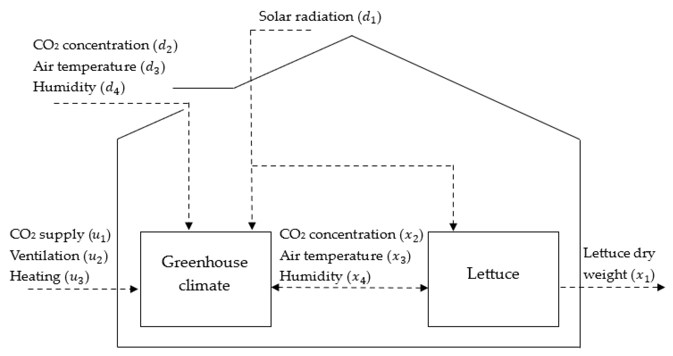
3. Lettuce Greenhouse Model

This work uses a validated greenhouse model by van Henten [7,8] to describe climate dynamics and lettuce growth. An overview of the model is presented in Figure 1. The model includes four state variables: lettuce dry weight (biomass), indoor CO₂ concentration, air temperature, and humidity. The control inputs are CO₂ injection rate, ventilation opening, and heating power. In Figure 1, labels and connections distinguish the control inputs, system measurements (derived from state variables), and external disturbances, with interactions represented by dashed lines. The discrete-time state-space model is formulated as:

$$\begin{array}{cc}\hfill x\left(k+1\right)& =f\left(x\left(k\right),u\left(k\right),d\left(k\right),p\right)\hfill \\ \hfill y\left(k\right)& =g\left(x\left(k\right),p\right)\hfill \end{array}$$

(1)

Here, $k\in Z^{+}$ denotes the discrete time, $x\left(k\right)\in R^{\mathrm{𝟜}}$ represents the state variables, $y\left(k\right)\in R^{\mathrm{𝟜}}$ is the output, $u\left(k\right)\in R^{\mathrm{𝟛}}$ denotes the control inputs, and $d\left(k\right)\in R^{\mathrm{𝟜}}$ represents the (weather) disturbances.

Table 1. Explanation of the state variables $x$, system outputs $y$, control inputs $u$, and weather disturbances $d$.

Category	Symbol	Description	Unit
State variables	$x_1$	Lettuce dry weight	kg/m2
	$x_2$	Indoor CO2 concentration	kg/m3
	$x_3$	Indoor Air temperature	°C
	$x_4$	Indoor Humidity	kg/m3
Measurement variables	$y_1$	Lettuce dry weight	g/m2
	$y_2$	Indoor CO2 concentration	ppm
	$y_3$	Indoor Air temperature	°C
	$y_4$	Indoor Humidity	%
Disturbances	$d_1$	Solar radiation	W/m2
	$d_2$	Outdoor CO2 concentration	kg/m3
	$d_3$	Outdoor Air temperature	°C
	$d_4$	Outdoor Humidity	kg/m3
Control inputs	$u_1$	CO2 supply	mg/m2/s
	$u_2$	Ventilation	mm/s
	$u_3$	Heating	W/m2

provides the meaning of all signals. The parameter vector $p\in R^{\mathrm{𝟚𝟠}}$, along with the nonlinear functions $f\left(\cdot \right)$ and $g\left(\cdot \right)$, is detailed in (2) and (4), respectively.

The dynamic model of the lettuce greenhouse is detailed with the nonlinear functions $f\left(\cdot \right)as$:

$$\left\{\begin{array}{l}{\displaystyle \frac{d{x}_1\left(t\right)}{dt}}=p_1{\varphi }_{phot,c}\left(t\right)-p_2{x}_1\left(t\right)2^{x_3\left(t\right)/10-5/2}\\ {\displaystyle \frac{d{x}_2\left(t\right)}{dt}}={\displaystyle \frac{1}{p_9}}\left(-{\varphi }_{phot,c}\left(t\right)+p_{10}{x}_1\left(t\right)2^{x_3\left(t\right)/10-5/2}+{{10}^{-6}u}_1\left(t\right)-{\varphi }_{\mathrm{vent},c}\left(t\right)\right)\\ {\displaystyle \frac{d{x}_3\left(t\right)}{dt}}={\displaystyle \frac{1}{p_{16}}}\left(u_3\left(t\right)-\left({{10}^{-3}p}_{17}{u}_2\left(t\right)+p_{18}\right)\left(x_3\left(t\right)-d_3\left(t\right)\right)+p_{19}{d}_1\left(t\right)\right)\\ {\displaystyle \frac{d{x}_4\left(t\right)}{dt}}={\displaystyle \frac{1}{p_{20}}}\left({\varphi }_{\mathrm{transp},h}\left(t\right)-{\varphi }_{\mathrm{vent},h}\left(t\right)\right)\end{array}\right.$$

(2)

with the flux terms are defined as:

$$\begin{array}{ccc}{\varphi }_{\mathit{phot},c}\left(t\right)& =& \left(1-e^{-p_3{x}_1\left(t\right)}\right){\displaystyle \frac{p_4{d}_1\left(t\right)\left(-p_5{x}_3^2\left(t\right)+p_6{x}_3\left(t\right)-p_7\right)\left(x_2\left(t\right)-p_8\right)}{p_4{d}_1\left(t\right)+\left(-p_5{x}_3^2\left(t\right)+p_6{x}_3\left(t\right)-p_7\right)\left(x_2\left(t\right)-p_8\right)}}\\ {\varphi }_{\mathit{transp},h}\left(t\right)& =& p_{21}\left(1-e^{-p_3{x}_1\left(t\right)}\right)\left({\displaystyle \frac{p_{22}}{p_{23}\left(x_3\left(t\right)+p_{24}\right)}}{e}^{{\displaystyle \frac{p_{25}{x}_3\left(t\right)}{x_3\left(t\right)+p_{26}}}}-x_4\left(t\right)\right)\\ {\varphi }_{\mathit{vent},c}\left(t\right)& =& \left({10}^{-3}{u}_2\left(t\right)+p_{11}\right)\left(x_2\left(t\right)-d_2\left(t\right)\right)\\ {\varphi }_{\mathit{vent},\mathrm{h}}\left(t\right)& =& \left({{10}^{-3}u}_2\left(t\right)+p_{11}\right)\left(x_4\left(t\right)-d_4\left(t\right)\right)\end{array}$$

(3)

Here, $t\in \mathbb{R}$ represents continuous time. The terms ${\varphi }_{\mathit{phot},c}\left(t\right), {\varphi }_{\mathit{vent},c}\left(t\right)$, ${\varphi }_{\mathit{transp},h}\left(t\right)$, and ${\varphi }_{\mathit{vent},h}\left(t\right)$ correspond to the gross photosynthesis rate, ${\mathrm{C}\mathrm{O}}_2$ mass exchange through ventilation, canopy transpiration, and ${\mathrm{H}}_2\mathrm{O}$ exchange through ventilation, respectively.

The output equations $g\left(\cdot \right)$ are defined as:

$$\left\{\begin{array}{ll}{y}_1\left(t\right)={10}^3\cdot x_1\left(t\right)& \hfill \mathrm{g}{\mathrm{m}}^{-2}\\ y_2\left(t\right)={\displaystyle \frac{{10}^6\cdot p_{12}\left(x_3\left(t\right)+p_{13}\right)}{p_{14}{p}_{15}}}\cdot x_2\left(t\right),& \hfill \mathrm{p}\mathrm{p}\mathrm{m}\\ y_3\left(t\right)=x_3\left(t\right),& \hfill °C\\ y_4\left(t\right)={\displaystyle \frac{{10}^2\cdot p_{12}\left(x_3\left(t\right)+p_{13}\right)}{11\cdot e^{\frac{p_{27}{x}_3\left(t\right)}{x_3\left(t\right)+p_{28}}}}}\cdot x_4\left(t\right),& \hfill \%\end{array}\right.$$

(4)

The specific values adopted for the model parameters $p$ are summarized in

Table 2. Model parameters and their values [7].

Symbol	Value	Unit	Explanation
p1	0.544	–	Yield Factor
p2	2.65 × 10−7	s−1	Maintenance Respiration
p3	53	m2·kg−1	Effective Canopy Area
p4	3.55 × 10−9	kg·J−1	PAR to total radiation conversion
p5	5.11 × 10−6	m·s−1·°C−2	Temp effect CO2, 2nd order
p6	2.3 × 10−4	m·s−1·°C−1	Temp effect CO2, 1st order
p7	6.29 × 10−4	m·s−1	Temp effect CO2, 0th order
p8	5.2 × 10−5	kg·m−3	CO2 compensation point
p9	4.1	m	Volumetric Capacity (CO2)
p10	4.87 × 10−7	s−1	Maintenance Respiration Weighted
p11	7.45 × 10−6	m·s−1	Leakage Greenhouse Cover
p12	8.314	J·K−1·mol−1	Gas Constant
p13	273.15	K	Absolute Temperature
p14	10,1325	Pa	Standard Atmospheric Pressure
p15	0.044	kg·mol−1	Molar Mass of CO2
p16	3 × 104	J·m−3·°C−1	Heat Capacity Greenhouse Air
p17	1290	J·m−3·°C−1	Heat Capacity Volume
p18	6.1	W·m−2·°C−1	Heat Transfer Coefficient
p19	0.2	–	Sun Heat Load Coefficient
p20	4.1	m	Volumetric Capacity (Humidity)
p21	0.0036	m·s−1	Canopy Transpiration Coefficient
p22	9348	J·kg−1·m−3·K−1	Water Molar Value (for transpiration)
p23	8314	J·K−1·mol−1	Gas Constant (water vapor)
p24	273.15	K	Absolute Temperature (humidity)
p25	17.4	–	Saturation Vapor Pressure (Canopy Transpiration)
p26	239	°C	Saturation Vapor Temp (Canopy Transpiration)
p27	17.269	–	Saturation Vapor Pressure (Humidity)
p28	238.3	°C	Saturation Vapor Temp (Humidity)

.

4. NMPC Formulation

This section details the NMPC framework employed for precision climate control in smart greenhouse environments. It outlines the specific control objectives, describes the economic and operational constraints, and the strategies used to integrate AI-based disturbance forecasting and real-time computational acceleration.

4.1. Control Objectives and Constraints

The primary objective of the NMPC controller is to maximize crop profitability while ensuring precision environmental control. This profit is defined as the revenue from the accumulated shoot biomass minus the operational costs associated with CO₂ injection and heating power usage. To formulate this control objective, an NMPC problem is defined as follows.

At each time instant $t$, the NMPC controller solves the following finite-horizon optimization problem:

$$\begin{array}{c}\underset{\left\{u\right(t+k\left|t\right),\hspace{0.17em}\epsilon (t+k|t){\}}_{k=0}^{N_p-1}}{\mathrm{m}\mathrm{i}\mathrm{n}}J\hfill \\ \mathrm{subject}\mathrm{to}\text{:}\hfill \\ x(t+k+1|t)=f\left(x(t+k|t),\hspace{0.17em}u(t+k\left|t\right),\hspace{0.17em}d(t+k|t)\right),\hfill \\ y(t+k|t)=g\left(x(t+k|t)\right),\hfill \\ u_{\mathrm{m}\mathrm{i}\mathrm{n}}\le u(t+k|t)\le u_{\mathrm{m}\mathrm{a}\mathrm{x}},\hfill \\ \left|u(t+k|t)-u(t+k-1\left|t\right)\right|\le \mathsf{\Delta }{u}_{\mathrm{m}\mathrm{a}\mathrm{x}},\hfill \\ y_{\mathrm{m}\mathrm{i}\mathrm{n}}(t+k)-\epsilon (t+k|t)\le y(t+k\left|t\right)\le y_{\mathrm{m}\mathrm{a}\mathrm{x}}(t+k)+\epsilon \left(t+k|t\right)\hfill \\ \epsilon (t+k|t)\ge 0,\hfill \\ \mathrm{for}k=0,\dots ,N_p-1.\hfill \end{array}$$

(5)

Here, $x(t+k|t)$ denotes the predicted state at time $t+k$ based on information available at time $t$, $u(t+k|t)$ is the control input, $d(t+k|t)$ is the disturbance prediction, $y(t+k|t)$ is the predicted output, and ${\epsilon }_j(t+k|t)$ are slack variables associated with the soft output constraints.

The cost function J to be minimized is given by:

$$\begin{gathered} J=\sum _{k=0}^{N_p-1}\left[-q_{y1}\cdot \left(y_1\left(t+k+1|t\right)-y_1\left(t+k|t\right)\right)+\sum _{i=1}^3{q}_{u_i}\cdot u_i\left(t+k|t\right) \\ +\sum _{i=1}^4{\rho }_i\cdot {\epsilon }_i^2\left(t+k+1|t\right)\right] \end{gathered}$$

(6)

where

$y_1(t+k|t)$ is the predicted shoot dry biomass at stage $t+k$ ($k=0,\dots ,N_p-1$).

$q_{y1}>0$ is the economic weight associated with incremental biomass production.

$q_{u_i}>0$ are economic weights reflecting the costs of CO₂ injection ($u_1$) and heating ($u_3$); ventilation ($u_2$) is omitted from penalization, as the employed model assumes natural ventilation with the ventilation rate determined by the window opening actuated by a motor; consequently, the energy cost associated with ventilation control is considered negligible [7,8,9].

${\rho }_i>0$ are penalty weights on the squared slack variables ${\epsilon }_i$ to regulate the extent and frequency of output constraint violations.

Penalty weight selection: In this study, the slack penalty weights for output constraints were not set to a single large value for all outputs, as is common in some related works. Instead, we assigned penalty weights inversely proportional to the amplitude of each output’s constraint bounds. This normalization ensures balanced treatment of constraint violations, regardless of output units or scales. For instance, outputs with large feasible ranges (e.g., biomass) are assigned smaller penalty weights, while those with narrow ranges (e.g., temperature, humidity) are assigned higher penalties. This strategy allows the optimizer to penalize relative violations consistently, improving interpretability and controlling fairness across heterogeneous outputs. Notably, the biomass constraint was always satisfied in all simulations, consistent with biological principles and the model structure; hence, its penalty was set arbitrarily high, with no effect on control outcomes. As a result, the penalties were set as follows: ρ₁ = 10⁵, ρ₂ = 10³, ρ₃ = 10⁵, ρ₄ = 10⁴.

Output Constraints: Time-varying constraints on temperature, humidity, and CO₂—adapted dynamically based on solar radiation—reflect horticultural best practices for energy-efficient regulation. The bounds for the full output vector are given by:

$$\begin{gathered} y_{\mathrm{m}\mathrm{i}\mathrm{n}}(t+k)={\left[0,\hspace{0.17em}{f}_{\mathrm{c}\mathrm{o}2,\mathrm{m}\mathrm{i}\mathrm{n}}(t+k),\hspace{0.17em}{f}_{\mathrm{t}\mathrm{e}\mathrm{m}\mathrm{p},\mathrm{m}\mathrm{i}\mathrm{n}}(t+k),\hspace{0.17em}50\right]}^T \\ {y}_{\mathrm{m}\mathrm{a}\mathrm{x}}(t+k)={\left[\mathrm{\infty },\hspace{0.17em}{f}_{\mathrm{c}\mathrm{o}2,\mathrm{m}\mathrm{a}\mathrm{x}}(t+k),\hspace{0.17em}{f}_{\mathrm{t}\mathrm{e}\mathrm{m}\mathrm{p},\mathrm{m}\mathrm{a}\mathrm{x}}(t+k),\hspace{0.17em}80\right]}^T \end{gathered}$$

(7)

Temperature bounds are time-varying functions of solar radiation $d_1(t+k|t)$:

$$\begin{array}{l}{f}_{\mathit{temp},\mathit{min}}\left(t+k\right)=\left\{\begin{array}{ll}10& \mathit{if}{d}_1(t+k|t)<10\mathrm{W}/{\mathrm{m}}^2\\ 22& \mathit{otherwise}\end{array}\right.\\ f_{\mathit{temp},\mathit{max}}\left(t+k\right)=\left\{\begin{array}{ll}15& \mathit{if}{d}_1(t+k|t)<10\mathrm{W}/{\mathrm{m}}^2\\ 27& \mathit{otherwise}\end{array}\right.\end{array}$$

(8)

CO₂ bounds are time-varying functions of solar radiation $d_1(t+k|t)$:

$$\begin{array}{l}{f}_{\mathrm{co}2,\mathit{min}}\left(t+k\right)=\left\{\begin{array}{ll}0& \mathit{if}{d}_1(t+k|t)<10\mathrm{W}/{\mathrm{m}}^2\\ 500& \mathit{otherwise}\end{array}\right.\\ f_{\mathrm{co}2,\mathit{max}}\left(t+k\right)=1600\end{array}$$

(9)

This radiation-dependent setpoint strategy aims to optimize crop growth conditions while promoting energy conservation, based on established horticultural principles. During periods of low incident solar radiation ($d_1(t+k|t)$ < 10 $\mathrm{W}/{\mathrm{m}}^2$), typically corresponding to night-time or heavily overcast conditions where photosynthetic activity is minimal, a cooler temperature range (10–15 °C for lettuce, as per Equation (8)) is maintained to reduce heating costs [29,30,31]. Conversely, under higher solar radiation levels, the permissible temperature range is elevated (22–27 °C, as per Equation (8)) to better support active photosynthesis, aligning with reported optimal daytime temperatures [29,30,31].

For CO₂ management (as Equation (9), a radiation-dependent approach sets the minimum concentration ($f_{\mathrm{co}2,\min }$) at 0 ppm during very low light conditions ($d_1(t+k|t)$ < 10 $\mathrm{W}/{\mathrm{m}}^2$), and 500 ppm otherwise, with an upper limit ($f_{\mathrm{co}2,\max }$) of 1600 ppm. This strategy, particularly the enrichment up to 1600 ppm during active photosynthesis, aligns with horticultural recommendations for optimal lettuce growth, which often suggest levels between 1000 and 1500 ppm [29,30], while reducing enrichment in low light conserves resources [30].

Furthermore, the relative humidity range of 50–80% is supported by findings suggesting optimal ranges within this span [29,30].

4.2. Disturbance Handling Approaches

Three approaches for handling external weather disturbances $d\left(k\right)$ within the NMPC framework are implemented:

• Feedback-Only Control (NMPC-C): This approach incorporates the currently measured disturbance $d\left(t\right)$ and assumes it remains constant over the entire prediction horizon $N_p$: $d(t+k\mid t)=d\left(t\right),$ for $k=0,\dots ,N_p-1$. This represents a reactive control strategy with no foresight.
• ML-Based Preview (NMPC-P): This controller utilizes current disturbance measurements $d\left(t\right|t)=d(t)$ for the initial control step ($k=0$). For the remainder of the prediction horizon ($k=1,\dots ,N_p-1$), it integrates multivariate disturbance forecasts generated by an LSTM neural network. Thus, the combined sequence matches the full NMPC prediction horizon.
  The LSTM leverages a sequence of recent historical disturbance measurements (defined by a lookback window of $L$ steps) to predict the future evolution of key weather variables ($d_1,\dots ,d_4$) over the subsequent $N_p-1$ steps.
  At each control interval, the NMPC controller collects the most recent $\mathrm{L}$ measurements of all disturbance variables, feeds them to the LSTM, receives a multi-step forecast of length ${\mathrm{N}}_{\mathrm{p}}-1$, and concatenates this forecast with the current measured disturbance to form the disturbance trajectory of length ${\mathrm{N}}_{\mathrm{p}}$ used in the NMPC optimization problem:

  $$\left[\mathrm{d}\right(\mathrm{t}\left|\mathrm{t}\right),\hspace{0.25em}\mathrm{d}(\mathrm{t}+1|\mathrm{t}),\hspace{0.25em}\dots ,\hspace{0.25em}\mathrm{d}(\mathrm{t}+{\mathrm{N}}_{\mathrm{p}}-1\left|\mathrm{t}\right)]$$
  Here, $\mathrm{d}\left(\mathrm{t}\right|\mathrm{t})$ is the current measured disturbance, and $\mathrm{d}(\mathrm{t}+\mathrm{k}|\mathrm{t})$ ($\mathrm{k}=1,\dots ,{\mathrm{N}}_{\mathrm{p}}-1$) are the LSTM-generated forecasts. Details on the LSTM architecture, input features, and training data are provided in Section 5.1.
• Ideal Preview (NMPC-I): This ideal scenario assumes perfect, error-free knowledge of future disturbances $d(t+k)$ over the prediction horizon. This serves as an upper-bound benchmark for the potential benefits of disturbance prediction.

The implementation of these strategies allows for a direct comparison of feedback, data-driven preview, and ideal disturbance information in greenhouse NMPC.

4.3. Warm-Start Initialization

To improve computational efficiency and solver convergence, a warm-start initialization strategy is employed for selected NMPC configurations (CW, PW, IW). At each control interval at time $t$, the optimal solution from the previous time step $t-1$ is used as the initial guess for the current optimization problem. The solution horizon shifted forward by one step, and the last value was duplicated to maintain horizon length.

Formally, if the previous solution was:

$$U_{t-1}^{\ast }=\left[u^{\ast }\right(t-1),\dots ,u^{\ast }(t-1+N_p-1\left)\right]$$

(10)

then the warm start at time $t$ is constructed as, denoted with a superscript (0):

$$U_t^{\left(0\right)}=\left[u^{\ast }\right(t),\dots ,u^{\ast }(t+N_p-2),u^{\ast }(t+N_p-2\left)\right]$$

(11)

This warm-start mechanism preserves the temporal structure of the control sequence and has been shown to substantially reduce solver iterations and computation time, particularly in scenarios with slow system dynamics or small setpoint changes. In this study, both cold-start and warm-start options are systematically compared across all disturbance-handling strategies to assess their impacts on computational and control performance.

5. Simulation Setup

This section details the generation of environmental disturbances, the performance metrics, the controller comparison approaches, and the parameters used for the NMPC simulations for evaluating the different control strategies.

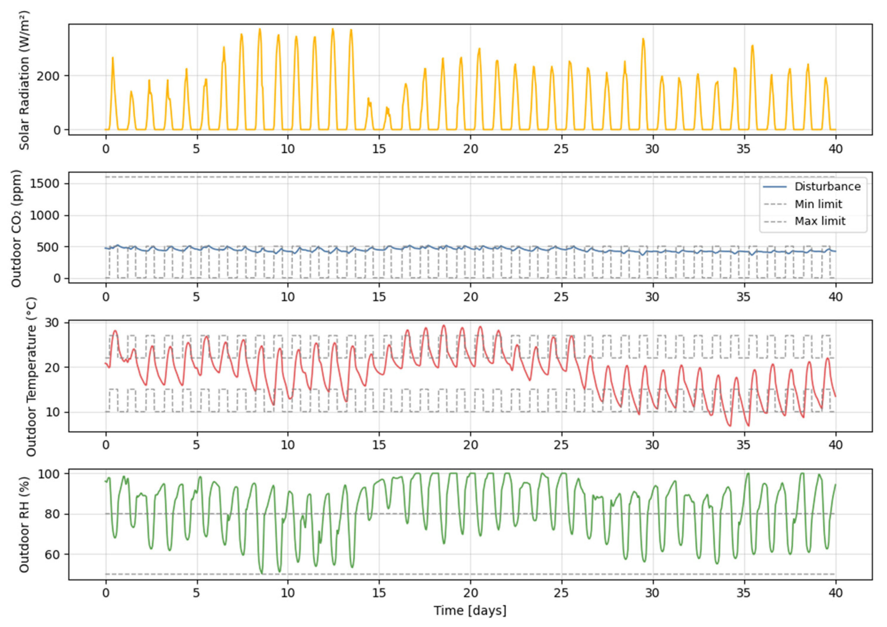
5.1. Disturbance Generation and Pre-Processing

The NMPC controllers were evaluated using realistic environmental disturbances generated as follows:

Outdoor air temperature, relative humidity, and global solar radiation data were retrieved from the NASA POWER (Prediction Of Worldwide Energy Resources) database [32] for the location of Thai Nguyen, Vietnam (21.5962° N, 105.8471° E). This database served as the source for two distinct datasets:

Simulation Dataset: For the purpose of controller evaluation via simulation, data were collected for the period 1 November 2020 to 10 December 2020 (40 days). This period was selected as it represents typical conditions for an early winter cultivation cycle in this region. The original hourly data for this 40-day period were linearly interpolated to achieve a 15 min resolution, matching the NMPC control interval.

LSTM Training and Validation Dataset: The LSTM model, responsible for generating weather previews (as described in Section 4.2), was trained and validated using historical data from the period 12 November 2016 to 31 October 2020 (i.e., all data prior to the simulation/test period). This extensive dataset was also processed to a 15 min resolution.

Daily averaged atmospheric CO₂ concentrations were initially extracted from OCO-2 (Orbiting Carbon Observatory 2) Level 3 data products [33]. To introduce more realistic diurnal variations crucial for greenhouse control, a Gaussian-modulated model was applied to these daily averages:

$${\mathrm{CO}}_2\left(t\right)=C_{base}+A{e}^{-{\displaystyle \frac{{\left(T_{out}-T_{opt}\right)}^2}{2{\sigma }^2}}}-\alpha R\left(t\right)$$

(12)

where

${\mathrm{CO}}_2\left(t\right)$ is the synthesized outdoor CO₂ concentration (ppm) at time t;

$C_{base}$: Base CO₂ concentration (daily averages) (ppm);

$A$: Scaling factor for temperature impact;

$T_{out}\left(t\right)$ is the outdoor temperature (°C);

$T_{opt}$: Optimal temperature for photosynthesis (°C);

$\sigma$: Standard deviation for temperature effect;

$\alpha$: Sensitivity factor for solar radiation impact;

$R\left(t\right)$: Incident solar radiation (W/m²).

The parameters were set as: A = 100, Topt = 22 °C, σ = 5, α = 0.04 ppm/(W/m²), chosen to reflect typical ambient variations and plant uptake influences, consistent with literature values for similar environments [29]. The resulting disturbance profiles used for the 40-day NMPC simulations are shown in Figure 2.

LSTM-based Weather Preview (for NMPC-P/PW): The 5.75 h (23-step) weather preview for the four disturbance variables ($d_1,d_2,d_3,d_4$) was generated using an LSTM model. The model architecture consisted of three LSTM layers with 128, 64, and 32 units, respectively. Dropout layers with a rate of 0.2 were included after the first two LSTM layers for regularization. These were followed by a separate dense output layer with a ReLU activation function for each predicted disturbance variable. The model used a lookback window of L = 20 steps (5 h) with 15 min interval data to predict the next W = 23 steps. The LSTM model was trained using an 80/10/10 train/validation/test split and optimized with the Adam algorithm, minimizing the mean squared error loss function. Training was conducted for up to 50 epochs, with a batch size of 32.

Upon completion of training, the LSTM disturbance forecast model demonstrated robust predictive performance across all weather variables.

Table 3. Predictive performance of the LSTM model on train, validation, and test sets.

Variable	MAE (Train)	RMSE (Train)	MAE (Valid)	RMSE (Valid)	MAE (Test)	RMSE (Test)
Solar Radiation (W/m2)	13.75	28.50	17.77	35.57	16.10	34.41
CO2 (ppm)	4.85	7.76	6.09	9.81	4.97	7.30
Temperature (°C)	0.58	0.93	0.62	1.01	0.70	1.17
Humidity (% RH)	2.23	3.54	2.45	3.99	2.92	4.61

summarizes the MAE and RMSE metrics for the train, validation, and test sets. Low error values were achieved for temperature, humidity, and CO₂, whereas higher errors were observed for solar radiation due to its greater variability.

5.2. Controller Comparison Approaches

To facilitate direct comparison,

Table 4. Summary of the NMPC controller variants evaluated.

Model	Disturbance Handling	Solver Initialization
NMPC-C	Frozen current disturbance $d\left(t\right)$	Cold-start
NMPC-CW	Frozen current disturbance $d\left(t\right)$	Warm-start
NMPC-P	LSTM-based disturbance prediction $d(t+k|t)$	Cold-start
NMPC-PW	LSTM-based disturbance prediction $d(t+k|t)$	Warm-start
NMPC-I	Ideal disturbance $d(t+k)$	Cold-start
NMPC-IW	Ideal disturbance $d(t+k)$	Warm-start

summarizes the six NMPC controller variants evaluated in this study. These configurations differ in their approaches to disturbance handling (feedback, ML-based preview, ideal preview) and solver initialization (cold-start, warm-start). This systematic classification enables a clear assessment of the individual and combined effects of forecast strategy and warm-start initialization on greenhouse control performance. Detailed analysis and discussion of these variants are provided in Section 6.

5.3. Performance Metrics

Controller performance was evaluated using the following KPIs:

Final Biomass ($B_f$, g/m²)

Total shoot dry mass of lettuce at harvest (end of simulation):

$$B_f=y_1\left(N_s\right)$$

(13)

where $y_1\left(k\right)$ is the shoot dry mass (g/m²) at simulation step $k$, and $N_s$ is the total number of simulation steps.

Net Profit ($P_{net}$, Hfl/m²)

Net profit is calculated as the revenue from harvested lettuce minus the total operating costs for CO₂ and heating:

$$P_{net}=R_{bio}-(C_{\mathrm{CO}2}+C_{heat})$$

(14)

where

Revenue from biomass ($R_{bio}$, Hfl/m²):

$$R_{bio}=c_p\cdot B_f\cdot {10}^{-3}$$

(15)

CO₂ cost ($C_{{\mathrm{C}\mathrm{O}}_2}$, Hfl/m²):

$$C_{{\mathrm{C}\mathrm{O}}_2}=c_{{\mathrm{C}\mathrm{O}}_2}\sum _{k=0}^{N_s-1}{u}_1(k)\mathsf{\Delta }t\cdot {10}^{-6}$$

(16)

Heating cost ($C_{heat}$, Hfl/m²):

$$C_{heat}=c_h\sum _{k=0}^{N_s-1}{u}_3(k)\mathsf{\Delta }t$$

(17)

where $c_p$ is the lettuce price (Hfl/kg), $c_{{\mathrm{C}\mathrm{O}}_2}$ the CO₂ cost (Hfl/kg), and $c_h$ the heating cost (Hfl/J). The term $B_f\cdot {10}^{-3}$ converts biomass from g/m² to kg/m²; $\sum u_1\left(k\right)\mathsf{\Delta }t\cdot {10}^{-6}$ is total CO₂ supplied (kg/m²); and $\sum u_3\left(k\right)\mathsf{\Delta }t$ is total heating energy used (J/m²). All other variables are as defined in Section 2.

Biomass Cost ($C_{bio}$, Hfl/kg)

Operating cost per kilogram of harvested biomass:

$$C_{bio}={\displaystyle \frac{C_{{\mathrm{C}\mathrm{O}}_2}+C_{heat}}{B_f\cdot {10}^{-3}}}$$

(18)

Constraint Violation Index ($V_i$, %)

The average normalized violation of each output constraint $y_i$, $i\in [1,4]$, is calculated as:

$$V_i={\displaystyle \frac{100}{N_s}}\sum _{k=0}^{N_s-1}{v}_i(k)$$

(19)

where the normalized violation at each time step $v_i\left(k\right)$ is defined as:

$$v_i(k)=\left\{\begin{array}{ll}0,& \mathrm{if}{y}_{i,\mathrm{m}\mathrm{i}\mathrm{n}}\left(k\right)\le y_i\left(k\right)\le y_{i,\mathrm{m}\mathrm{a}\mathrm{x}}\left(k\right)\\ {\displaystyle \frac{y_i\left(k\right)-y_{i,\mathrm{m}\mathrm{a}\mathrm{x}}\left(k\right)}{y_{i,\mathrm{m}\mathrm{a}\mathrm{x}}\left(k\right)-y_{i,\mathrm{m}\mathrm{i}\mathrm{n}}\left(k\right)}},& \mathrm{if}{y}_i\left(k\right)>y_{i,\mathrm{m}\mathrm{a}\mathrm{x}}\left(k\right)\\ {\displaystyle \frac{y_{i,\mathrm{m}\mathrm{i}\mathrm{n}}\left(k\right)-y_i\left(k\right)}{y_{i,\mathrm{m}\mathrm{a}\mathrm{x}}\left(k\right)-y_{i,\mathrm{m}\mathrm{i}\mathrm{n}}\left(k\right)}},& \mathrm{if}{y}_i\left(k\right)<y_{i,\mathrm{m}\mathrm{i}\mathrm{n}}\left(k\right)\end{array}\right.$$

(20)

where $y_i\left(k\right)$ is the value of output $i$ at time step $k$, and $y_{i,\mathrm{m}\mathrm{a}\mathrm{x}}\left(k\right)$, $y_{i,\mathrm{m}\mathrm{i}\mathrm{n}}\left(k\right)$ are its time-varying upper and lower bounds, respectively.

The primary indices reported are: $V_B=V_1$, $V_C=V_2$, $V_T=V_3$, $V_H=V_4$.

Aggregated Constraint Violation Index ($V_{total},\%$)

An aggregated measure of all individual constraint violation indices:

$$V_{total}=\sum _{i=1}^4{V}_i$$

(21)

This value provides an overall measure of constraint adherence.

Average Solver Time ($T_{sol}$, s)

The mean CPU time required by the IPOPT solver to find the solution to the NMPC optimization problem at each control interval.

5.4. Simulation Parameters

Key parameters for the NMPC simulations are summarized in

Table 5. Core simulation parameters for NMPC evaluation.

Parameter	Symbol	Value
1. Time-related parameters
Sampling time	$\mathsf{\Delta }t$	15 min (900 s)
NMPC Prediction horizon	$N_p$	24 steps (6 h)
NMPC Control horizon	$N_c$	24 steps (6 h)
Simulation duration	$N_s$	40 days (3840 control steps)
2. Model/Controller parameters
Numerical solver	-	IPOPT (via CasADi)
Initial crop dry weight	$x_1\left(t_0\right)$	0.0035 kg/m2 (3.5 g/m2)
Initial indoor CO2 concentration	$x_2\left(t_0\right)$	0.001 kg/m3 (~400 ppm at 15 °C)
Initial indoor temperature	$x_3\left(t_0\right)$	15 °C
Initial indoor humidity	$x_4\left(t_0\right)$	0.008 kg/m3 (~65% RH)
Initial state of control inputs	$u(t_0-1)$	(0, 0, 0)T
Economic weight: Biomass	$q_{y1}$	2800
Economic weight: CO2 input	$q_{u1}$	66
Economic weight: Heating input	$q_{u3}$	1
Slack variable penalty: Biomass	${\rho }_1$	105
Slack variable penalty: CO2	${\rho }_2$	103
Slack variable penalty: Temp.	${\rho }_3$	105
Slack variable penalty: Humid.	${\rho }_4$	104
Lower bounds for control inputs	$u_{min}$	(0, 0, 0)T
Upper bounds for control inputs	$u_{max}$	(12 mg/m2/s, 75 mm/s, 150 W/m2)T
Max. rate of change inputs	$\mathsf{\Delta }{u}_{max}$	(1.2, 7.5, 15)T (units/step)
3. Economic cost coefficients
Lettuce price	$c_p$	1.6 Hfl kg−1
Heating energy cost	$c_h$	$6.35\times {10}^{-9}$ Hfl J−1
CO2 cost	$c_{\mathrm{C}{\mathrm{O}}_2}$	0.42 Hfl kg−1

. The prediction horizon ($N_p=24$ steps, 6 h) was selected to effectively capture daily environmental variability, enabling proactive climate control while maintaining computational feasibility at a 15 min control interval. This horizon also aligns with the effective forecast window of typical short-term weather prediction models [21,23].

Economic weights in the objective function were chosen to prioritize biomass accumulation ${(q}_{y1})$, while relatively smaller weights for CO₂ injection ${(q}_{u1})$ and heating input $\left(q_{u3}\right)$ were assigned to penalize excessive resource consumption, reflecting their operational costs and promoting resource efficiency (Equation (6)). The control signal ranges and rate limits are based on standard actuator capacities and established horticultural practices for lettuce production [18,20,21]. Cost coefficients for profit calculation, including lettuce price and unit costs for heating energy and CO₂, are adopted from the literature [18,20].

The nonlinear optimization problem arising from the NMPC formulation is solved using a direct multiple shooting approach, implemented in Python (version 3.11.9) via the CasADi automatic differentiation framework [34]. The IPOPT solver [35] is used for nonlinear programming. The system dynamics (Equations (1)–(3)) are discretized using a fixed-step forward Euler method with a sampling time of 15 min (900 s), which also corresponds to the control interval. For controller configurations that employ warm-start initialization (Section 4.3), IPOPT’s warm-start features are activated by providing the shifted solution from the previous time step as the initial guess. All simulations are run on an Intel i7-4810MQ CPU with 20GB RAM.

6. Results and Discussion

This section presents and discusses the comparative performance of the six NMPC configurations (C, CW, P, PW, I, and IW) detailed in Section 5.2. The evaluation focuses on agronomic outcomes (biomass yield, constraint satisfaction), economic efficiency (net profit, operational costs), and computational performance (solver time). The discussion is organized based on two primary timescales: short-term (first 3 days) and full-cycle (40 days), followed by a general discussion of trade-offs and controller selection.

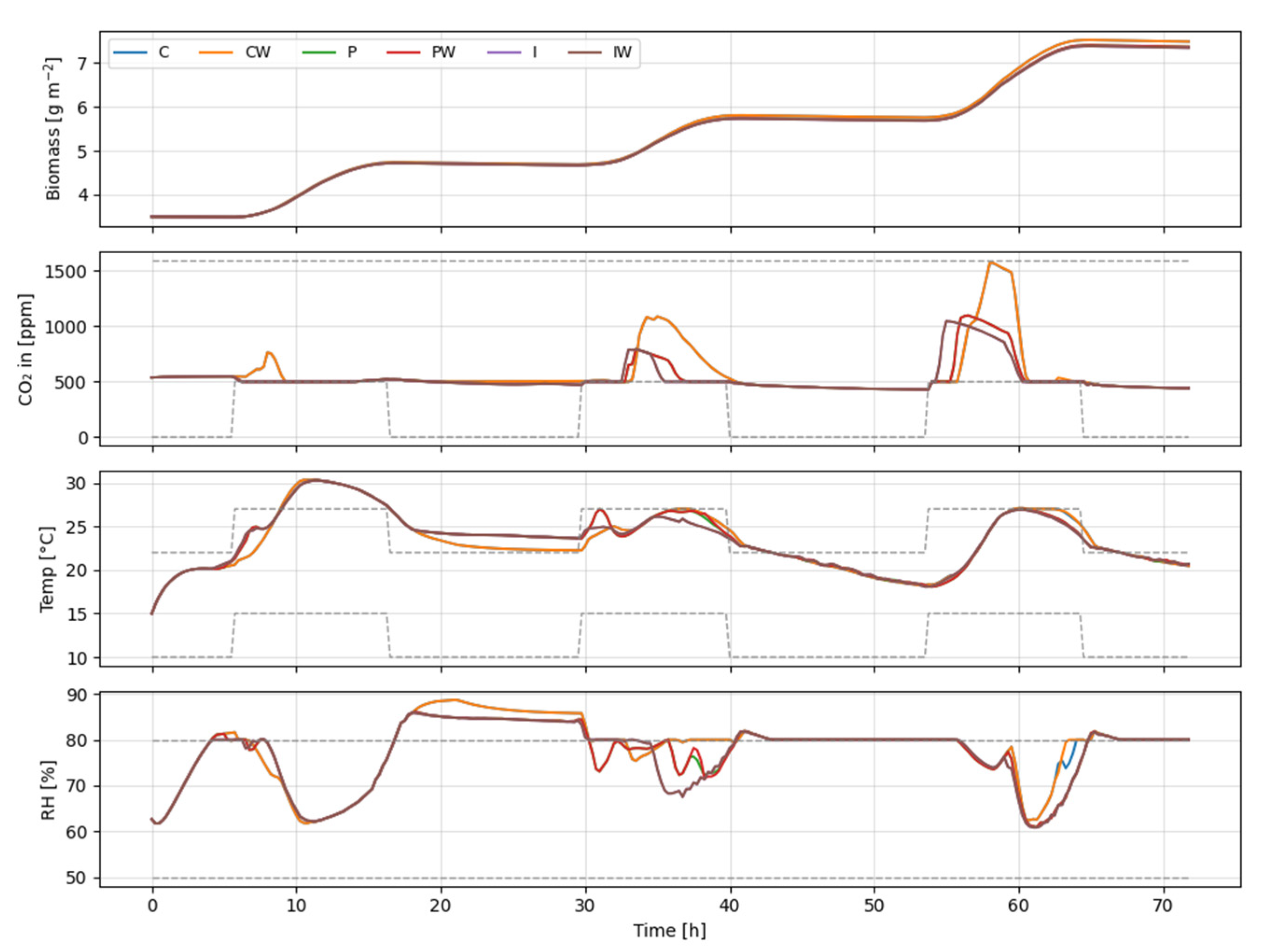
6.1. Short-Term (3-Day) Performance

Figure 3 presents the time evolution of four key system outputs—biomass, internal CO₂ concentration, temperature, and relative humidity—over a 72 h simulation for six NMPC configurations (C, CW, P, PW, I, IW). The biomass plot shows similar growth patterns among all controllers, indicating comparable crop development. The CO₂ concentration plot reveals that C and CW maintain higher and more stable daytime CO₂ levels, supporting enhanced photosynthetic activity, while the other configurations regulate CO₂ more conservatively. The temperature and humidity plots demonstrate that all controllers keep these variables within safe bounds, with some fluctuations corresponding to environmental changes and control actions. Overall, this figure highlights the ability of all NMPC configurations to maintain suitable conditions for crop growth, with clear differences in resource management and environmental stability.

Figure 4 illustrates the control signals generated by the NMPC controllers for CO₂ injection, ventilation, and heating during the same simulation period for the six configurations. The C and CW controllers apply CO₂ in large, stable pulses, while the predictive configurations (P, PW, I, IW) use smaller, more frequent, and dispersed doses to optimize CO₂ usage. Ventilation signals show that C and CW often adopt an on/off approach, whereas the predictive controllers adjust ventilation with higher frequency and smaller amplitude to more precisely regulate the internal climate. Heating is activated in cycles, mainly during cooler periods, with predictive controllers exhibiting more frequent and flexible power adjustments. These results demonstrate distinct control strategies, where C and CW focus on maximizing growth, while P, PW, I, and IW prioritize efficient resource utilization and operational cost savings.

Table 6. KPIs over the first 3 days.

Model	${\mathit{B}}_{\mathit{f}}$ (g m−2)	${\mathit{V}}_{\mathit{t}\mathit{o}\mathit{t}\mathit{a}\mathit{l}}$ (%)	${\mathit{V}}_{\mathit{C}}$ (%)	${\mathit{V}}_{\mathit{T}}$ (%)	${\mathit{V}}_{\mathit{H}}$ (%)	${\mathit{C}}_{\mathit{b}\mathit{i}\mathit{o}}$ (Hfl/kg)	${\mathit{P}}_{\mathit{n}\mathit{e}\mathit{t}}$ (Hfl m−2)	${\mathit{T}}_{\mathit{s}\mathit{o}\mathit{l}}$ (s)
NMPC-C	7.489	8.710	0.022	4.328	4.360	5.533	0.098	0.489
NMPC-CW	7.490	8.707	0.022	4.323	4.362	5.534	0.098	0.299
NMPC-P	7.369	8.785	0.030	5.688	3.067	7.931	0.087	1.188
NMPC-PW	7.369	8.785	0.030	5.689	3.066	7.952	0.087	0.404
NMPC-I	7.347	8.661	0.030	5.683	2.948	8.321	0.086	0.897
NMPC-IW	7.348	8.661	0.030	5.683	2.948	8.322	0.086	0.302

summarizes the short-term performance (first 72 h) of all six NMPC controllers. Final biomass after 3 days is highest for NMPC-C and NMPC-CW controllers (7.489 and 7.490 g/m²), slightly higher than for the predictive (P, PW: 7.369 g/m²) and ideal controllers (I, IW: 7.347, 7.348 g/m²). Total constraint violation ($V_{total}$) is similar across all controllers (≈8.7%). The average solver time is substantially reduced in warm-started controllers (CW: 0.299 s, PW: 0.404 s, IW: 0.302 s) compared to their non-warm-started counterparts (C: 0.489 s, P: 1.188 s, I: 0.897 s). Furthermore, for each pair of controllers with and without warm-start, the output values are nearly identical, as visually confirmed by the almost overlapping trajectories in Figure 3 and Figure 4, and quantitatively reinforced by the summarized data in Table 6, where performance metrics such as biomass, constraint violations, and profit differ by less than 0.1% between each pair. This demonstrates that, under the tested conditions, the use of warm-start mainly improves computational efficiency without significantly affecting the control quality or agronomic outcomes. For subsequent full-cycle analysis, only the warm-started controllers (CW, PW, IW) are visualized for clarity.

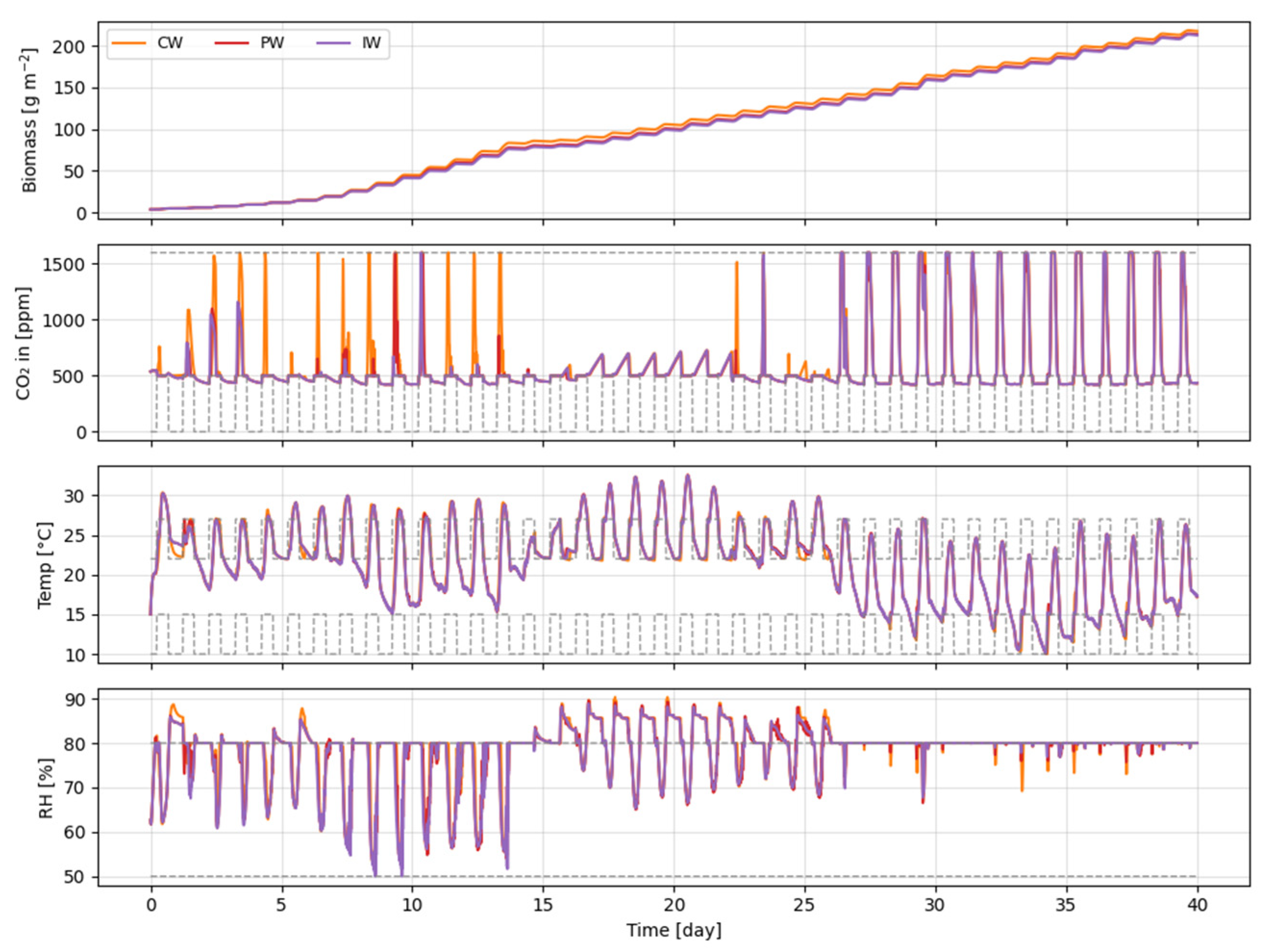
6.2. Full Horizon (40-Day) Performance

The full 40-day cultivation cycle simulation provided comprehensive performance data for all six NMPC controller variants.

Table 7. Full-cycle (40-day) performance of all controller strategies.

Model	${\mathit{B}}_{\mathit{f}}$ (g m−2)	${\mathit{V}}_{\mathit{t}\mathit{o}\mathit{t}\mathit{a}\mathit{l}}$ (%)	${\mathit{V}}_{\mathit{C}}$ (%)	${\mathit{V}}_{\mathit{T}}$ (%)	${\mathit{V}}_{\mathit{H}}$ (%)	${\mathit{C}}_{\mathit{b}\mathit{i}\mathit{o}}$ (Hfl/kg)	${\mathit{P}}_{\mathit{n}\mathit{e}\mathit{t}}$ (Hfl m−2)	${\mathit{T}}_{\mathit{s}\mathit{o}\mathit{l}}$ (s)
NMPC-C	217.362	6.861	0.054	3.758	3.049	3.833	2.658	0.457
NMPC-CW	217.459	6.866	0.054	3.700	3.112	3.815	2.663	0.320
NMPC-P	213.584	6.630	0.055	3.756	2.819	3.932	2.591	1.041
NMPC-PW	213.585	6.628	0.054	3.755	2.819	3.931	2.592	0.396
NMPC-I	212.472	6.479	0.046	3.594	2.839	3.894	2.586	0.908
NMPC-IW	212.492	6.480	0.046	3.598	2.836	3.899	2.585	0.308

presents the KPIs, including final biomass, constraint violation indices, net profit, and average solver times. Figure 5, Figure 6, Figure 7, Figure 8, Figure 9, Figure 10 and Figure 11 offer detailed visualizations of the system’s dynamic behavior, economic outcomes, constraint adherence, resource utilization, and computational performance across these configurations.

6.2.1. Disturbance Handling Strategy Performance

As detailed in Table 7, NMPC-C and NMPC-CW achieved the highest final biomass (approximately 217.4 g m⁻² and 217.5 g m⁻², respectively) and, consequently, the highest net profit (approximately 2.658 Hfl m⁻² and 2.663 Hfl m⁻², respectively). This superior productivity can be attributed to the controllers’ tendency to maintain high CO₂ concentrations during periods of sufficient light, thereby maximizing photosynthetic activity, as evidenced by the higher assimilation rates shown in Figure 10. However, this reactive and aggressive approach—due to the controllers’ lack of future disturbance information—resulted in the highest rates of constraint violations among all strategies, particularly for temperature and humidity setpoints (Figure 8). While these controllers incurred the greatest operational costs related to CO₂ injection (Figure 7 and Figure 9), their heating costs were lower than those of the predictive controllers (Figure 7). This suggests that C and CW responded only to current conditions and did not proactively increase heating in anticipation of future humidity or temperature violations. Despite higher CO₂ consumption, their biomass cost ($C_{bio}$) remains competitive due to substantial yield gains.

The integration of future disturbance information, whether from an ML-based preview (P, PW) or an ideal forecast (I, IW), enabled these controllers to proactively adjust control actions in anticipation of upcoming environmental fluctuations. As a result, they achieved lower overall constraint violations—particularly for temperature and relative humidity—compared to the feedback-only controllers (Figure 8). This improved constraint adherence was primarily accomplished through more conservative CO₂ dosing as well as strategic increases in heating to preempt periods of elevated humidity or temperature (Figure 6). While these controllers reduced total CO₂ costs (Figure 7 and Figure 9), they exhibited slightly higher heating costs than their feedback-only counterparts (Figure 7), reflecting a deliberate trade-off between resource efficiency and stricter climate control.

6.2.2. Warm-Start Initialization Performance

Across all disturbance handling approaches, warm-starting the solver (CW, PW, IW) consistently yielded substantial improvements in computational efficiency without adverse effects on agronomic or economic outcomes. Average solver times, as shown in Table 7 and Figure 11, were reduced by approximately 30–60% compared to their cold-start counterparts. For instance, NMPC-CW (0.320 s) was considerably faster than NMPC-C (0.457 s), and NMPC-IW (0.308 s) outperformed NMPC-I (0.908 s). This reduction in both the mean and variance of solver times is crucial for ensuring the feasibility and reliability of NMPC in real-time greenhouse operations. The warm-started controllers (CW, PW, IW) exhibited both lower average solver times and a more concentrated distribution of solution times compared to their non-warm-started counterparts, as illustrated in Figure 11.

6.3. Discussion of Trade-Offs and Controller Selection

The comparative analysis conducted in Section 6.2 clearly reveals a fundamental trade-off inherent in the selection of NMPC strategies. On one hand, feedback-only controllers (C, CW) excel at maximizing final yield and profit by aggressively managing CO₂ enrichment and overall climate conditions to consistently favor robust plant growth. However, this approach inherently leads to higher CO₂ consumption and a greater tendency for the system to operate at or occasionally slightly beyond predefined operational constraint boundaries (Figure 8 and Figure 9). Heating expenditures for these controllers are generally lower, as they do not proactively compensate for future environmental changes (Figure 7). On the other hand, predictive controllers (P, PW, I, IW) demonstrate superior performance in minimizing constraint violations and reducing CO₂ costs (Figure 7 and Figure 8). This enhanced efficiency and constraint safety is achieved through more cautious and anticipatory control actions, supported by access to future disturbance information, albeit typically involving a modest sacrifice in maximum potential yield, and consequently, net profit (Table 7). This observed trade-off between productivity and strict constraint adherence is a common challenge in greenhouse climate control, as highlighted by recent studies [15,20].

The choice of an optimal NMPC strategy should therefore be guided by the specific operational priorities and economic context of the greenhouse. If maximizing output is paramount and the system can tolerate minor deviations from setpoints, NMPC-CW presents a compelling option due to its high yield, profitability, and computational efficiency. This aligns with recent research emphasizing yield optimization in horticulture [20]. If, however, strict adherence to climate setpoints, energy conservation, or CO₂ emission reduction is the primary concern, a predictive strategy such as NMPC-PW may be more suitable, offering a favorable balance between proactive control, resource savings, and computational feasibility. The ideal preview controllers (I, IW) serve as important theoretical benchmarks, highlighting the potential gains from perfect foresight. The results also suggest that while the economic weights in the NMPC objective function influence the trade-off between productivity and resource use, the penalty factors for constraint violations predominantly determine the overall degree of constraint violation and play a crucial role in ensuring system safety. With appropriately tuned penalties, all evaluated controllers maintained the greenhouse environment within broadly acceptable limits for lettuce cultivation.

To evaluate the practical implications of measurement uncertainty, we conducted a sensitivity analysis examining how a ±10% error in final biomass ($B_f$) estimation impacts net profit calculations for each NMPC controller. Our findings, summarized in

Table 8. Net profit ($P_{net}$) intervals for all controller strategies, accounting for ±10% biomass measurement error.

Controller	$\mathbf{Nominal}{\mathit{P}}_{\mathit{n}\mathit{e}\mathit{t}}$ (Hfl/m2)	${\mathit{P}}_{\mathit{n}\mathit{e}\mathit{t}}^{+10\mathbf{\%}}$ (Hfl/m2)	${\mathit{P}}_{\mathit{n}\mathit{e}\mathit{t}}^{-10\mathbf{\%}}$ (Hfl/m2)
NMPC-C	2.658	2.893	2.423
NMPC-CW	2.663	2.898	2.428
NMPC-P	2.591	2.821	2.361
NMPC-PW	2.592	2.822	2.362
NMPC-I	2.586	2.815	2.356
NMPC-IW	2.585	2.815	2.356

, show that while net profit is linearly related to $B_f$ (Equations (14) and (15)) and, thus, fluctuates directly with measurement error, the relative ranking of controller performance remains robust. This indicates that our main conclusions are valid even under realistic measurement uncertainties in crop yield, reinforcing the robustness of the proposed NMPC strategies for practical application.

7. Conclusions

This study comprehensively evaluated advanced NMPC strategies integrating AI-driven components for climate control in smart greenhouse systems, emphasizing the impacts of disturbance prediction and warm-start initialization through extensive 40-day simulations of a lettuce greenhouse model across six distinct controller configurations. The findings revealed a clear trade-off: controllers employing only real-time feedback (NMPC-C, NMPC-CW) consistently maximized final biomass and profit by maintaining elevated CO₂ levels, which facilitated greater CO₂ assimilation; however, this approach also increased constraint violations. Conversely, strategies utilizing LSTM-based disturbance prediction (NMPC-P, NMPC-PW) or ideal foresight (NMPC-I, NMPC-IW) demonstrated improved resource efficiency and enhanced adherence to operational constraints, often by adopting more cautious CO₂ supplementation, albeit at the expense of slightly lower yields. Crucially, warm-start initialization proved highly effective across all controller types, significantly reducing average solver computation times by up to 60% without any discernible impact on control performance or output quality, thereby underscoring its practical value for real-time automation in smart greenhouse control. Furthermore, the study highlighted that while economic objective weights influence the balance between productivity and resource expenditure, the satisfaction of operational constraints is predominantly governed by the selection of appropriate penalty parameters. The selection of an optimal NMPC strategy should therefore be guided by specific operational priorities, whether that is maximizing yield and economic returns, minimizing resource consumption and environmental impact, or strictly enforcing climate setpoints; regardless of the chosen control logic, the adoption of warm-start techniques is strongly recommended to ensure computational feasibility in practical real-time AI-driven smart greenhouse applications.

While this research provides valuable insights, its foundation on simulation-based evaluations using a specific lettuce crop model, a validated greenhouse climate model from Wageningen Agricultural University, and particular environmental conditions (Thai Nguyen, Vietnam) underscores the necessity for further investigation. Key limitations include the simplification of real-world atmospheric CO₂ dynamics and microclimate variations by the synthetic CO₂ model and gridded NASA POWER weather data, respectively, as well as the use of a pre-trained, static ML-based weather predictor. Additionally, the NMPC formulation did not incorporate online model parameter adaptation to address potential model–plant mismatch over extended cultivation periods, focused on a single set of tuning parameters (economic weights and constraint penalties), excluded the energy cost associated with natural ventilation as it is considered negligible in the assumed model, and excluded considerations of external economic factors like market price volatility or detailed physiological aspects such as air circulation’s impact on tipburn. Building upon these limitations, future research should prioritize on-site experimental validation in diverse greenhouse settings and across different crop types. Developing adaptive NMPC frameworks that integrate online learning for both process models and disturbance predictors, performing comprehensive sensitivity analyses for tuning parameters, and incorporating broader economic and parametric uncertainties will be crucial for advancing more resilient, efficient, and economically optimal greenhouse control systems for sustainable horticulture.

References

1. Findeisen, R.; Allgöwer, F. An Introduction to Nonlinear Model Predictive Control. In Proceedings of the 21st Benelux Meeting on Systems and Control, Veldhoven, The Netherlands, 19–21 March 2002; pp. 119–141. [Google Scholar]
2. Kouvaritakis, B.; Cannon, M. Model Predictive Control: Classical, Robust and Stochastic; Springer: Berlin/Heidelberg, Germany, 2016. [Google Scholar]
3. García-Mañas, F.; Rodríguez, F.; Berenguel, M.; Maestre, J.M. Multi-Scenario Model Predictive Control for Greenhouse Crop Production Considering Market Price Uncertainty. IEEE Trans. Autom. Sci. Eng. 2024, 21, 2936–2948. [Google Scholar] [CrossRef]
4. Esparza-Gómez, J.M.; Guerrero-Osuna, H.A.; Ornelas-Vargas, G.; Luque-Vega, L.F. RNN-LSTM Applied in a Temperature Prediction Model for Greenhouses. Res. Comput. Sci. 2021, 150, 31–41. [Google Scholar]
5. Chen, L.; Han, B.; Wang, X.; Zhao, J.; Yang, W.; Yang, Z. Machine Learning Methods in Weather and Climate Applications: A Survey. Appl. Sci. 2023, 13, 12019. [Google Scholar] [CrossRef]
6. Diehl, M.; Bock, H.G.; Schlöder, J.P. A Real-Time Iteration Scheme for Nonlinear Optimization in Optimal Feedback Control. SIAM J. Control Optim. 2005, 43, 1714–1736. [Google Scholar] [CrossRef]
7. Van Henten, E.J. Greenhouse Climate Management: An Optimal Control Approach; Landbouwuniversiteit Wageningen: Wageningen, The Netherlands, 1994. [Google Scholar]
8. Van Henten, E.J. Sensitivity Analysis of an Optimal Control Problem in Greenhouse Climate Management. Biosyst. Eng. 2003, 85, 355–364. [Google Scholar] [CrossRef]
9. Van Henten, E.J.; Bontsema, J. Time-Scale Decomposition of an Optimal Control Problem in Greenhouse Climate Management. Control Eng. Pract. 2009, 17, 88–96. [Google Scholar] [CrossRef]
10. Blasco, X.; Martinez, M.; Herrero, J.M.; Ramos, C.; Sanchis, J. Model-Based Predictive Control of Greenhouse Climate for Reducing Energy and Water Consumption. Comput. Electron. Agric. 2007, 55, 49–70. [Google Scholar] [CrossRef]
11. Mahmood, F.; Govindan, R.; Bermak, A.; Yang, D.; Al-Ansari, T. Data-Driven Robust Model Predictive Control for Greenhouse Temperature Control and Energy Utilisation Assessment. Appl. Energy 2023, 343, 121190. [Google Scholar] [CrossRef]
12. Hu, G.; You, F. AI-Enabled Cyber-Physical-Biological Systems for Smart Energy Management and Sustainable Food Production in a Plant Factory. Appl. Energy 2024, 356, 122334. [Google Scholar] [CrossRef]
13. Gruber, J.K.; Guzmán, J.L.; Rodríguez, F.; Bordons, C.; Berenguel, M.; Sánchez, J.A. Nonlinear MPC Based on a Volterra Series Model for Greenhouse Temperature Control Using Natural Ventilation. Control Eng. Pract. 2011, 19, 354–366. [Google Scholar] [CrossRef]
14. Boersma, S.; Sun, C.; Van Mourik, S. Robust Sample-Based Model Predictive Control of a Greenhouse System with Parametric Uncertainty. In Proceedings of the IFAC AGRICONTROL 2022, Munich, Germany, 14–16 September 2022. [Google Scholar]
15. Svensen, J.L.; Cheng, X.; Boersma, S.; Sun, C. Chance-Constrained Stochastic MPC of Greenhouse Production Systems with Parametric Uncertainty. Comput. Electron. Agric. 2024, 217, 108578. [Google Scholar] [CrossRef]
16. Zavala, V.M.; Biegler, L.T. The Advanced-Step NMPC Controller: Optimality, Stability and Robustness. Automatica 2009, 45, 86–93. [Google Scholar] [CrossRef]
17. Gros, S.; Zanon, M. Data-Driven Economic NMPC Using Reinforcement Learning. IEEE Trans. Automat. Control 2020, 65, 636–648. [Google Scholar] [CrossRef]
18. Mallick, S.; Airaldi, F.; Dabiri, A.; Sun, C.; De Schutter, B. Reinforcement Learning-Based Model Predictive Control for Greenhouse Climate Control. Smart Agric. Technol. 2025, 10, 100751. [Google Scholar] [CrossRef]
19. Mallick, S.; Airaldi, F.; Dabiri, A.; Sun, C.; De Schutter, B. Deep Neural Network Based Optimal Control of Greenhouses. In Proceedings of the 2024 European Control Conference (ECC), Stockholm, Sweden, 25–28 June 2024. [Google Scholar] [CrossRef]
20. Morcego, B.; Yin, W.; Boersma, S.; Van Henten, E.; Puig, V.; Sun, C. Reinforcement Learning Versus Model Predictive Control on Greenhouse Climate Control. Comput. Electron. Agric. 2023, 215, 108372. [Google Scholar] [CrossRef]
21. Jansen, Y.T.G. Optimal Control of Lettuce Greenhouse Horticulture Using Model-Free Reinforcement Learning: An Investigation on the Effect of Short-Term Weather Forecast Horizons. Master’s Thesis, Utrecht University, Utrecht, The Netherlands, 2022. [Google Scholar]
22. Kuijpers, W.J.P.; Antunes, D.J.; Van Mourik, S.; Van Henten, E.J.; Van De Molengraft, M.J.G. Weather Forecast Error Modelling and Performance Analysis of Automatic Greenhouse Climate Control. Biosyst. Eng. 2022, 214, 207–229. [Google Scholar] [CrossRef]
23. Zhang, H.; Liu, Y.; Zhang, C.; Li, N. Machine Learning Methods for Weather Forecasting: A Survey. Atmosphere 2025, 16, 82. [Google Scholar] [CrossRef]
24. Boersma, S.; Cheng, X. A Bayesian Neural ODE for a Lettuce Greenhouse. In Proceedings of the 2024 IEEE Conference on Control Technology and Applications (CCTA), Newcastle upon Tyne, UK, 21–23 August 2024; pp. 782–786. [Google Scholar] [CrossRef]
25. Zavala, V.M.; Anitescu, M. Real-Time Nonlinear Optimization as a Generalized Equation. SIAM J. Control Optim. 2010, 48, 5444–5467. [Google Scholar] [CrossRef]
26. Quirynen, R.; Vukov, M.; Zanon, M.; Diehl, M. Autogenerating Microsecond Solvers for Nonlinear MPC: A Tutorial Using ACADO Integrators. Optim. Control Appl. Methods 2014, 36, 685–704. [Google Scholar] [CrossRef]
27. Kirches, C.; Wirsching, L.; Bock, H.G.; Schlöder, J.P. Efficient Direct Multiple Shooting for Nonlinear Model Predictive Control on Long Horizons. J. Process. Control 2012, 22, 540–550. [Google Scholar] [CrossRef]
28. Gros, S.; Mario, Z.; Rien, Q.; Alberto, B.; Diehl, M. From Linear to Nonlinear MPC: Bridging the Gap via the Real-time Iteration. Int. J. Control 2016, 93, 62–80. [Google Scholar] [CrossRef]
29. Ahmed, H.A.; Yu-Xin, T.; Qi-Changa, Y. Optimal Control of Environmental Conditions Affecting Lettuce Plant Growth in a Controlled Environment with Artificial Lighting: A Review. S. Afr. J. Bot. 2020, 130, 75–89. [Google Scholar] [CrossRef]
30. Brechner, M.; Both, A.J.; Staff, C.E.A. Hydroponic Lettuce Handbook; Cornell University CEA Program: Ithaca, NY, USA, 2013. [Google Scholar]
31. Dai, M.; Tan, X.; Ye, Z.; Ren, J.; Chen, X.; Kong, D. Optimal Light Intensity for Lettuce Growth, Quality, and Photosynthesis in Plant Factories. Plants 2024, 13, 2616. [Google Scholar] [CrossRef] [PubMed]
32. Zhang, T.; Chandler, W.S.; Hoell, J.M.; Westberg, D.; Whitlock, C.H.; Stackhouse, P.W. A Global Perspective on Renewable Energy Resources: Nasa’s Prediction of Worldwide Energy Resources (Power) Project. In Proceedings of the Proceedings of ISES World Congress 2007 (Vol. I–Vol. V), Beijing, China, 8–21 September 2007; Goswami, D.Y., Zhao, Y., Eds.; Springer: Berlin/Heidelberg, Germany, 2009; pp. 2636–2640. [Google Scholar]
33. Brad Weir, L.O. and O.-2 S.T. OCO-2 GEOS Level 3 Daily, 0.5×0.625 Assimilated CO2 V10r. Available online: https://oco2.gesdisc.eosdis.nasa.gov/ (accessed on 15 April 2025).
34. Andersson, J.A.E.; Gillis, J.; Horn, G.; Rawlings, J.B.; Diehl, M. CasADi: A Software Framework for Nonlinear Optimization and Optimal Control. Math. Program. Comput. 2019, 11, 1–36. [Google Scholar] [CrossRef]
35. Wächter, A.; Biegler, L.T. On the Implementation of an Interior-Point Filter Line-Search Algorithm for Large-Scale Nonlinear Programming. Math Program. 2006, 106, 25–57. [Google Scholar] [CrossRef]
Figure 1. The employed lettuce greenhouse model [7].
Applsci 15 07988 g001
Figure 2. Disturbance Profiles used in 40-day greenhouse NMPC simulations. Dashed gray lines indicate lower and upper operational limits for CO2, temperature, and RH, enabling direct visual assessment of when and how much the external disturbances violate desired setpoints.
Applsci 15 07988 g002
Figure 3. System outputs for all six NMPC controllers over the first 3 days of simulation. Gray dashed lines indicate operational bounds for CO2, temperature, and RH.
Applsci 15 07988 g003
Figure 4. System control signals for all six NMPC controllers over the first 3 days of simulation.
Applsci 15 07988 g004
Figure 5. System outputs over the full 40-day cycle for three representative warm-started NMPC controllers (CW, PW, IW). Gray dashed lines show operational constraints for CO2, temperature, and RH.
Applsci 15 07988 g005
Figure 6. System control actions over the full 40-day cycle for three representative warm-started NMPC controllers (CW, PW, IW).
Applsci 15 07988 g006
Figure 7. Bar chart of key economic performance indicators for all NMPC controllers: CO2 cost, heating cost, and total biomass revenue.
Applsci 15 07988 g007
Figure 8. Stacked bar chart of constraint violations for all NMPC controllers, decomposed into CO2, temperature, and relative humidity components.
Applsci 15 07988 g008
Figure 9. Trade-off between final biomass yield and total CO2 cost for all NMPC controllers over the 40-day cycle.
Applsci 15 07988 g009
Figure 10. CO2 budget decomposition for each NMPC configuration, showing total CO2 supplied, CO2 lost through ventilation, and CO2 assimilated by the crop.
Applsci 15 07988 g010
Figure 11. Histogram of solver times for each NMPC configuration over the 40-day simulation horizon. Warm-started controllers (CW, PW, IW) achieve lower and more concentrated solve times.
Applsci 15 07988 g011