A SkSP-R Plan under the Assumption of Gompertz Distribution

Abstract

In this study, we designed a time-truncated SkSP-R sampling plan when the lifetime of units follows a Gompertz distribution (GmzD). The GmzD is briefly discussed. All of the plan parameters were obtained using a two-point approach, which is based on limiting quality level (LQL) and acceptable quality level (AQL). Moreover, operating characteristic (OC) values were calculated for the determined value of the plan parameters by using the OC function of the SkSP-R. Applications of two real life situations in engineering were presented to illustrate the applicability of the offered sampling inspection plan. It was found that the new SkSP-R sampling inspection plan can be used efficiently in the field.

1. Introduction

The industry directly depends on customers and their experiences about the product quality. Thus, the quality of the product is the most important factor in making the product more demanding to the customers by manufacturing units. To provide consumers a positive impression of product quality, a manufacturer or wholesaler selects the highest-quality product from a lot and distributes it to customers.. For the selection of best quality product, one may use 100 percent inspection, but 100 percent inspection is not possible due to time, money, labor, etc., constraints. In addition to 100 percent inspection, we have a path between 100 percent inspection and no inspection that is known as acceptance sampling inspection plan (ASIP). Various types of ASIPs are presented in the literature; namely; attribute ASIP and variable ASIP, Single ASIP (SASIP), double ASIP (DASIP), multiple ASIP (MASIP), sequential ASIP (SeASIP), group ASIP (GASIP), and skip-lot ASIP (SkASIP) are included in attribute ASIP, while sampling plans are based on variables using perfect measurements of quality characteristics.

Some of the authors who have developed several ASIPs for different probability distributions include the following: Ref. [1] for gamma distribution, Ref. [2] for for normal and lognormal distributions, Ref. [3] for Birnbaum Saunders model, Ref. [4] for inverse Rayleigh distribution, Ref. [5] for generalized Rayleigh distribution, Ref. [6] for generalized Birnbaum Saunders model, Ref. [7] for generalized exponential distribution, Ref. [8] for generalized inverted exponential distribution, Ref. [9] for for SASIP based on generalized half-normal distribution and [10] for SASIP and DASIP to the transmuted Rayleigh distribution, Ref. [11] for chain sampling plan for variables inspection, Ref. [12] for selection of chain sampling plans ChSP-1 and ChSP-(0,1). Moreover, see [13,14,15,16,17,18,19,20,21,22,23,24,25,26,27,28,29,30] for other works in ASP.

We explored the literature of SQC and found that this is the first study developing SkSP-R under the GmzD. In addition, we placed a strong emphasis on the suggested plan’s real implementation, and we employed two data sets to accomplish this goal. The structure of this paper is classified as follows: In Section 2, GmzD is presented with its main properties. The design of the offered SkSP-R plan for GmzD is placed in Section 3 along with illustration. The description of tables is provided in Section 4. Real data set examples for application purposes are presented in Section 5. Section 6 summarizes the main finding and concludes the paper.

2. Gompertz Distribution

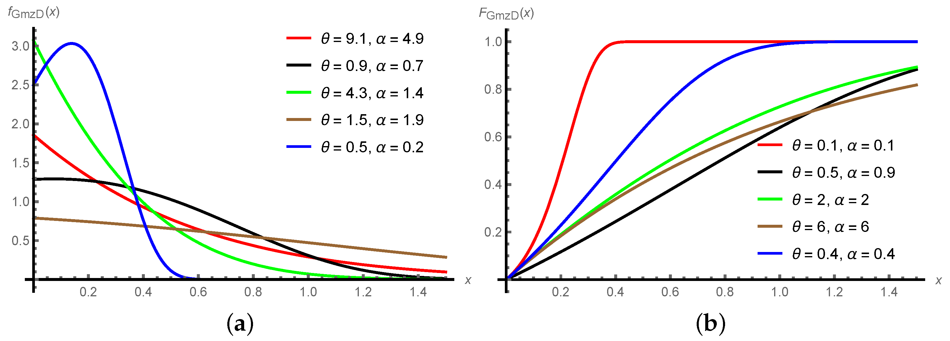
The Gompertz distribution is introduced by Benjamin Gompertz in 1825 and showed the importance of GmzD by considering human mortality and actuarial tables. The GmzD is a an extended version of the exponential distribution and it has a relationship with double exponential, exponential, generalized logistic, Weibull, and extreme value (Gumbel) distributions. The probability density function (pdf) and cumulative distribution function cdf of the GmzD are provided below, respectively, as:

$$f\left(x\right)=\frac{\theta }{\alpha }{e}^{x/\alpha }{e}^{-\theta (e^{x/\alpha }-1)};x>0,\theta >0,\alpha >0,$$

(1)

and

$$F\left(x\right)=1-e^{-\theta (e^{x/\alpha }-1)}.$$

(2)

The mean of the GmzD is as follows.

$$\mu =\alpha e^{\theta }\mathrm{\Gamma }(0,\theta ).$$

(3)

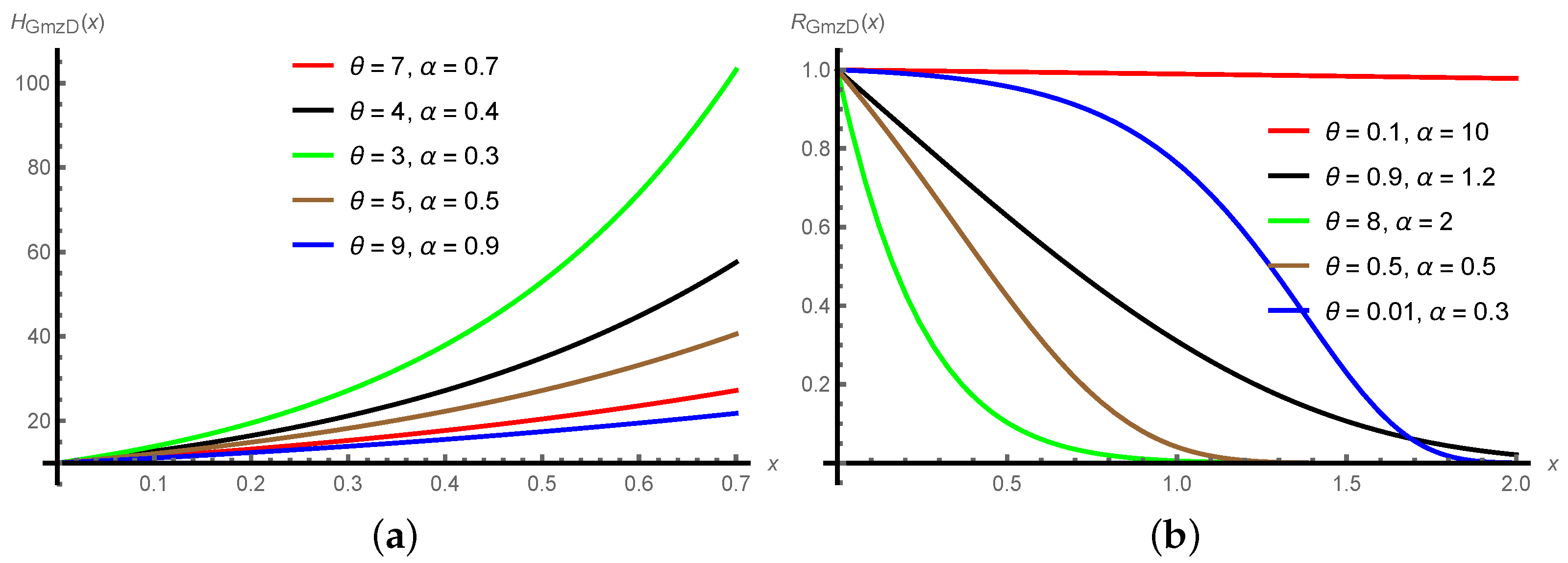
The hazard rate and reliability functions of the GmzD are, respectively, given by the following.

$$H\left(x\right)=\frac{\theta e^{x/\alpha }}{\alpha },\mathrm{and}R\left(x\right)=e^{\theta -\theta e^{x/\alpha }}.$$

The plots of the probability density and cumulative distribution functions of the GmzD are provided in Figure 1 for some selected parameters. Moreover, the plots of the hazard rate and reliability functions of the GmzD are provided in Figure 2 for various parameters choices. Figure 2 revealed the flexibility of the GmzD in accommodating several shapes of the hazard rate and reliability functions.

3. Design of the SkSP-R Plan for GmzD

This section defines and discusses the SkSP-R for the GmzD distribution considered in this study. SkSP-R is introduced by [31] and showed its advantages over some other popular ASIPs. The SkSP-R plan parameters are ($n,c,i,f,k$, and m). The procedure of time truncated SkSP-R can be described as follows:

1.

Begin with the normal inspection using the reference plan, and then place n items on test for prefixed time $t_0$. Notice and count the number of sample items that failed before the experiment duration, say, d. If $d\le c$, then accept the lot and reject it if $d>c$.

2.

Stop the normal inspection and utilize the skipping inspection (SI) if i successive units are accepted under normal inspection based on time truncated life tests.

3.

Within SI, inspect only a fraction f of lots that is randomly selected. SI is continued until a sampled lot is rejected.

4.

If a lot is not accepted after k consecutively sampled lots have been accepted, then the resampling procedure is employed for the immediate next lot as given below (Step 5).

5.

Within the resampling technique, conduct the inspection based on the reference plan and continue SI if the lot is accepted. If the lot is not accepted, resampling is performed m times and the lot is rejected if it has not accepted on $(m-1)$st resubmission.

6.

If a lot is not accepted based on resampling scheme, then directly revert to the normal inspection (Step 1).

7.

Remove or correct all the nonconforming units found with conforming units in the rejected lots.

The average sample number (ASN) of the SkSP-R is as follows:

$$ASN=\frac{nfQ{P}^{i+k}-nf{P}^k(1-P^i)(1-Q^m)+nf}{P^i(1+fQ{P}^k)+f(1-P^i)[1-P^k(1-Q^m)]},$$

(4)

and the OC function probability od acceptance of the proposed SkSP-R is as follows:

$$P_a=\frac{(1-f)P^i+f{P}^k(P^i-P)(1-Q^m)+fP}{P^i(1+fQ{P}^k)+f(1-P^i)[1-P^k(1-Q^m)]},$$

(5)

where $P={\sum }_{j=0}^c\left(\genfrac{}{}{0pt}{}{n}{j}\right)p^j{(1-p)}^{n-j}$, and $p=F\left(t_0\right)$ is the CDF of GmzD, which can be modified in terms of termination ratio and quality ratio as follows.

$$p=1-e^{-\theta [e^{(t_0/{\mu }_0)\times (e^{\theta }\mathrm{\Gamma }(0,\theta )/\mu /{\mu }_0)}-1]}.$$

(6)

Now, we employed a two-point strategy to determine plan parameters; in this approach, the OC curve passes through both AQL and LQL. As a result, the optimization problem for determining plan parameters using the two-point technique AQL and LQL, as well as the optimization problem, is the following:

$$ASN=\frac{nfQ{P}^{i+k}-nf{P}^k(1-P^i)(1-Q^m)+nf}{P^i(1+fQ{P}^k)+f(1-P^i)[1-P^k(1-Q^m)]},$$

(7)

$$\frac{f{P}_0+(1-f)P_0^i+f{P}_0^k(P_0^i-P_0)(1-Q_0^m)}{f(1-P_0^i)[1-P_0^k(1-Q_0^m)]+P_0^i(1+f{Q}_0{P}_0^k)}\ge 1-{\alpha }_p,$$

(8)

$$\begin{array}{c}\hfill \frac{f{P}_1+(1-f)P_1^i+f{P}_1^k(P_1^i-P_1)(1-Q_1^m)}{f(1-P_1^i)[1-P_1^k(1-Q_1^m)]+P_1^i(1+f{Q}_1{P}_1^k)}\le \beta ,\end{array}$$

(9)

where $P_0$ and $P_1$ are probabilities at AQL and LQL, with $Q_0$ and $Q_1$ being $1-P_0$ and $1-P_1$, respectively. Our aim is to minimize the ASN of proposed SkSP-R where ASN depends on the sample size n. Therefore, we minimize the sample size by using the above mentioned optimization problem (Equations (6)–(8)).

4. Description of Tables

To demonstrate how the proposed SkSP-R would be implemented, some tables are presented and discussed for various plan parameters. The necessary tables for values of $\theta =2,3,4,5$, $m=2$, $\beta =0.25,0.05,0.10,0.01$, ${\alpha }_p=0.10$, termination ratio $t_0/{\mu }_0=0.5,0.75$, $m=2$, and quality ratio ($\mu /{\mu }_0$ is $2,3,4,5,6,7$, and 8) are computed. Plan parameters and probability of lot acceptance for $\theta =2,3,4,5$ are placed in

Table 1. Plan parameters of SkSP-R for GmzD with $\theta =2$ and $m=2$.

		$\mathit{a}={\mathit{t}}_0/{\mathit{\mu }}_0=0.5$							$\mathit{a}={\mathit{t}}_0/{\mathit{\mu }}_0=0.75$
$\mathbf{\beta }$	$\mathbf{\mu }/{\mathbf{\mu }}_{\mathbf{0}}$	n	c	i	f	k	${\mathbf{P}}_{\mathit{acg}}\left(\mathit{p}\right)$	ASN	n	c	i	f	k	${\mathbf{P}}_{\mathit{acg}}\left(\mathit{p}\right)$	ASN
0.25	2	34	10	2	$0.5$	1	$0.9535057$	$27.97392$	24	10	2	$0.5$	1	$0.9553009$	$20.06413$
	3	31	9	2	$0.5$	1	$0.9959384$	$25.66619$	22	9	2	$0.5$	1	$0.9960654$	$18.66366$
	4	28	8	2	$0.5$	1	$0.9990554$	$21.41822$	19	8	2	$0.5$	1	$0.9994029$	$15.21178$
	5	24	7	2	$0.5$	1	$0.9996647$	$19.1525$	17	7	2	$0.5$	1	$0.9996928$	$13.84022$
	6	21	6	2	$0.5$	1	$0.9997141$	$16.87444$	15	6	2	$0.5$	1	$0.9997168$	$12.43753$
	7	18	5	2	$0.5$	1	$0.9996190$	$14.58213$	13	5	2	$0.5$	1	$0.9995891$	$10.99879$
	8	15	4	2	$0.5$	1	$0.9992690$	$12.27287$	11	4	2	$0.5$	1	$0.9991400$	$9.517559$
0.10	2	68	18	2	$0.5$	1	$0.9625093$	$66.06291$	47	18	2	$0.5$	1	$0.9689919$	$45.63715$
	3	64	17	2	$0.5$	1	$0.9994385$	$61.85672$	45	17	2	$0.5$	1	$0.9994789$	$43.85736$
	4	61	16	2	$0.5$	1	$0.9999713$	$59.12137$	42	16	2	$0.5$	1	$0.9999815$	$40.61462$
	5	58	15	2	$0.5$	1	$0.9999963$	$56.36989$	40	15	2	$0.5$	1	$0.9999976$	$38.85132$
	6	54	14	2	$0.5$	1	$0.9999993$	$52.20480$	38	14	2	$0.5$	1	$0.9999993$	$37.06218$
	7	51	13	2	$0.5$	1	$0.9999997$	$49.46471$	35	13	2	$0.5$	1	$0.9999998$	$33.86162$
	8	48	12	2	$0.5$	1	$0.9999998$	$46.70592$	33	12	2	$0.5$	1	$0.9999998$	$32.0866$
0.05	2	114	30	2	$0.5$	1	$0.9895492$	$113.1479$	79	30	2	$0.5$	1	$0.9917155$	$78.44711$
	3	110	29	2	$0.5$	1	$0.9999873$	$109.0512$	76	29	2	$0.5$	1	$0.9999924$	$75.32948$
	4	107	28	2	$0.5$	1	$0.9999999$	$106.1515$	74	28	2	$0.5$	1	$1.0000000$	$73.42533$
	5	104	27	2	$0.5$	1	$1.0000000$	$103.2452$	72	27	2	$0.5$	1	$1.0000000$	$71.51112$
	6	100	26	2	$0.5$	1	$1.0000000$	$99.16030$	69	26	2	$0.5$	1	$1.0000000$	$68.40539$
	7	97	25	2	$0.5$	1	$1.0000000$	$96.25778$	67	25	2	$0.5$	1	$1.0000000$	$66.49731$
	8	93	24	2	$0.5$	1	$1.0000000$	$92.17513$	65	24	2	$0.5$	1	$1.0000000$	$64.57880$
0.01	2	154	38	2	$0.5$	1	$0.9857021$	$153.9443$	106	38	2	$0.5$	1	$0.9893034$	$105.9631$
	3	151	37	2	$0.5$	1	$0.9999931$	$150.9517$	104	37	2	$0.5$	1	$0.999996$	$103.9696$
	4	147	36	2	$0.5$	1	$1.0000000$	$146.9463$	101	36	2	$0.5$	1	$1.0000000$	$101.9751$
	5	144	35	2	$0.5$	1	$1.0000000$	$143.9537$	99	35	2	$0.5$	1	$1.0000000$	$98.96939$
	6	140	34	2	$0.5$	1	$1.0000000$	$139.9486$	97	34	2	$0.5$	1	$1.0000000$	$96.97509$
	7	137	33	2	$0.5$	1	$1.0000000$	$136.9561$	94	33	2	$0.5$	1	$1.0000000$	$93.96941$
	8	133	32	2	$0.5$	1	$1.0000000$	$132.9513$	92	32	2	$0.5$	1	$1.0000000$	$91.97531$

,

Table 2. Plan parameters of SkSP-R for GmzD with $\theta =3$ and $m=2$.

		$\mathit{a}={\mathit{t}}_0/{\mathit{\mu }}_0=0.5$							$\mathit{a}={\mathit{t}}_0/{\mathit{\mu }}_0=0.75$
$\mathbf{\beta }$	$\mathbf{\mu }/{\mathbf{\mu }}_{\mathbf{0}}$	n	c	i	f	k	${\mathbf{P}}_{\mathit{acg}}\left(\mathit{p}\right)$	ASN	n	c	i	f	k	${\mathbf{P}}_{\mathit{acg}}\left(\mathit{p}\right)$	ASN
$0.25$	2	32	10	2	$0.5$	1	$0.9538064$	$25.85492$	23	10	2	$0.5$	1	$0.952789$	$18.9601$
	3	29	9	2	$0.5$	1	$0.9960467$	$23.39951$	21	9	2	$0.5$	1	$0.9957579$	$17.49022$
	4	26	8	2	$0.5$	1	$0.9991216$	$20.95096$	19	8	2	$0.5$	1	$0.9989842$	$16.0018$
	5	23	7	2	$0.5$	1	$0.9995944$	$18.50952$	17	7	2	$0.5$	1	$0.9994881$	$14.49266$
	6	20	6	2	$0.5$	1	$0.9996732$	$16.07547$	15	6	2	$0.5$	1	$0.9995471$	$12.96005$
	7	17	5	2	$0.5$	1	$0.9995915$	$13.64909$	12	5	2	$0.5$	1	$0.9996393$	$9.617745$
	8	14	4	2	$0.5$	1	$0.9992689$	$11.23064$	10	4	2	$0.5$	1	$0.9992878$	$8.138429$
$0.10$	2	64	18	2	$0.5$	1	$0.9623296$	$61.82625$	45	18	2	$0.5$	1	$0.966264$	$43.48126$
	3	61	17	2	$0.5$	1	$0.9992944$	$59.01565$	43	17	2	$0.5$	1	$0.9993888$	$41.68839$
	4	58	16	2	$0.5$	1	$0.9999636$	$56.20086$	41	16	2	$0.5$	1	$0.9999678$	$39.87927$
	5	55	15	2	$0.5$	1	$0.9999954$	$53.38140$	39	15	2	$0.5$	1	$0.9999958$	$38.05390$
	6	52	14	2	$0.5$	1	$0.9999988$	$50.55674$	36	14	2	$0.5$	1	$0.9999993$	$34.79924$
	7	48	13	2	$0.5$	1	$0.9999996$	$46.32888$	34	13	2	$0.5$	1	$0.9999997$	$32.99749$
	8	45	12	2	$0.5$	1	$0.9999997$	$43.52742$	32	12	2	$0.5$	1	$0.9999997$	$31.17690$
$0.05$	2	108	30	2	$0.5$	1	$0.9883012$	$107.1027$	76	30	2	$0.5$	1	$0.9897322$	$75.41146$
	3	105	29	2	$0.5$	1	$0.9999810$	$104.1692$	74	29	2	$0.5$	1	$0.9999846$	$73.48365$
	4	102	28	2	$0.5$	1	$0.9999999$	$101.2336$	72	28	2	$0.5$	1	$0.9999999$	$71.54970$
	5	99	27	2	$0.5$	1	$1.0000000$	$98.29585$	69	27	2	$0.5$	1	$1.0000000$	$68.42994$
	6	95	26	2	$0.5$	1	$1.0000000$	$94.17864$	67	26	2	$0.5$	1	$1.0000000$	$66.50477$
	7	92	25	2	$0.5$	1	$1.0000000$	$91.24830$	65	25	2	$0.5$	1	$1.0000000$	$64.57284$
	8	89	24	2	$0.5$	1	$1.0000000$	$88.31538$	62	24	2	$0.5$	1	$1.0000000$	$61.45723$
$0.01$	2	147	38	2	$0.5$	1	$0.9813676$	$146.9547$	103	38	2	$0.5$	1	$0.9833812$	$102.9737$
	3	143	37	2	$0.5$	1	$0.9999908$	$142.9469$	100	37	2	$0.5$	1	$0.9999934$	$99.96625$
	4	140	36	2	$0.5$	1	$1.0000000$	$139.9523$	98	36	2	$0.5$	1	$1.0000000$	$97.97152$
	5	137	35	2	$0.5$	1	$1.0000000$	$136.9574$	95	35	2	$0.5$	1	$1.0000000$	$94.96343$
	6	133	34	2	$0.5$	1	$1.0000000$	$132.9501$	93	34	2	$0.5$	1	$1.0000000$	$92.96930$
	7	130	33	2	$0.5$	1	$1.0000000$	$129.9556$	91	33	2	$0.5$	1	$1.0000000$	$90.97441$
	8	127	32	2	$0.5$	1	$1.0000000$	$126.9607$	88	32	2	$0.5$	1	$1.0000000$	$87.96706$

,

Table 3. Plan parameters of SkSP-R for GmzD with $\theta =4$ and $m=2$.

		$\mathit{a}={\mathit{t}}_0/{\mathit{\mu }}_0=0.5$							$\mathit{a}={\mathit{t}}_0/{\mathit{\mu }}_0=0.75$
$\mathbf{\beta }$	$\mathbf{\mu }/{\mathbf{\mu }}_{\mathbf{0}}$	n	c	i	f	k	${\mathbf{P}}_{\mathit{acg}}\left(\mathit{p}\right)$	ASN	n	c	i	f	k	${\mathbf{P}}_{\mathit{acg}}\left(\mathit{p}\right)$	ASN
$0.25$	2	31	10	2	$0.5$	1	$0.9529443$	$24.90356$	23	10	2	$0.5$	1	$0.9405765$	$19.56785$
	3	28	9	2	$0.5$	1	$0.9960064$	$22.35642$	21	9	2	$0.5$	1	$0.9943247$	$18.00976$
	4	26	8	2	$0.5$	1	$0.9987942$	$21.7716$	18	8	2	$0.5$	1	$0.9991692$	$14.39786$
	5	23	7	2	$0.5$	1	$0.9994509$	$19.19575$	16	7	2	$0.5$	1	$0.9995955$	$12.89812$
	6	20	6	2	$0.5$	1	$0.9995685$	$16.63486$	14	6	2	$0.5$	1	$0.9996545$	$11.38677$
	7	17	5	2	$0.5$	1	$0.9994774$	$14.08994$	12	5	2	$0.5$	1	$0.9995407$	$9.861995$
	8	14	4	2	$0.5$	1	$0.9990974$	$11.56217$	10	4	2	$0.5$	1	$0.9991243$	$8.321259$
$0.10$	2	63	18	2	$0.5$	1	$0.9539819$	$61.27592$	45	18	2	$0.5$	1	$0.9529552$	$43.95910$
	3	60	17	2	$0.5$	1	$0.9990669$	$58.40179$	42	17	2	$0.5$	1	$0.999305$	$40.65008$
	4	56	16	2	$0.5$	1	$0.9999619$	$54.08897$	40	16	2	$0.5$	1	$0.9999629$	$38.82681$
	5	53	15	2	$0.5$	1	$0.9999953$	$51.23819$	38	15	2	$0.5$	1	$0.9999951$	$36.99133$
	6	50	14	2	$0.5$	1	$0.9999988$	$48.38748$	36	14	2	$0.5$	1	$0.9999987$	$35.1434$
	7	47	13	2	$0.5$	1	$0.9999995$	$45.53644$	33	13	2	$0.5$	1	$0.9999996$	$31.88039$
	8	44	12	2	$0.5$	1	$0.9999997$	$42.68460$	31	12	2	$0.5$	1	$0.9999997$	$30.05944$
$0.05$	2	105	30	2	$0.5$	1	$0.9869442$	$104.1437$	75	30	2	$0.5$	1	$0.9864446$	$74.53027$
	3	102	29	2	$0.5$	1	$0.9999773$	$101.1917$	72	29	2	$0.5$	1	$0.9999828$	$71.39263$
	4	99	28	2	$0.5$	1	$0.9999999$	$98.23924$	70	28	2	$0.5$	1	$0.9999999$	$69.46043$
	5	96	27	2	$0.5$	1	$1.0000000$	$95.28632$	68	27	2	$0.5$	1	$1.0000000$	$67.52334$
	6	93	26	2	$0.5$	1	$1.0000000$	$92.33283$	66	26	2	$0.5$	1	$1.0000000$	$65.58145$
	7	90	25	2	$0.5$	1	$1.0000000$	$89.37870$	63	25	2	$0.5$	1	$1.0000000$	$62.45506$
	8	86	24	2	$0.5$	1	$1.0000000$	$85.25299$	61	24	2	$0.5$	1	$1.0000000$	$60.52318$
$0.01$	2	142	38	2	$0.5$	1	$0.9810519$	$141.9459$	100	38	2	$0.5$	1	$0.9832736$	$99.96297$
	3	139	37	2	$0.5$	1	$0.9999883$	$138.9502$	98	37	2	$0.5$	1	$0.9999906$	$97.96809$
	4	136	36	2	$0.5$	1	$1.0000000$	$135.9543$	96	36	2	$0.5$	1	$1.0000000$	$95.97265$
	5	133	35	2	$0.5$	1	$1.0000000$	$132.9582$	94	35	2	$0.5$	1	$1.0000000$	$93.97670$
	6	130	34	2	$0.5$	1	$1.0000000$	$129.9619$	92	34	2	$0.5$	1	$1.0000000$	$91.98028$
	7	126	33	2	$0.5$	1	$1.0000000$	$125.9539$	89	33	2	$0.5$	1	$1.0000000$	$88.97385$
	8	123	32	2	$0.5$	1	$1.0000000$	$122.9582$	87	32	2	$0.5$	1	$1.0000000$	$86.97798$

and

Table 4. Plan parameters of SkSP-R for GmzD with $\theta =5$ and $m=2$.

		$\mathit{a}={\mathit{t}}_0/{\mathit{\mu }}_0=0.5$							$\mathit{a}={\mathit{t}}_0/{\mathit{\mu }}_0=0.75$
$\mathbf{\beta }$	$\mathbf{\mu }/{\mathbf{\mu }}_{\mathbf{0}}$	n	c	i	f	k	${\mathbf{P}}_{\mathit{acg}}\left(\mathit{p}\right)$	ASN	n	c	i	f	k	${\mathbf{P}}_{\mathit{acg}}\left(\mathit{p}\right)$	ASN
$0.25$	2	31	10	2	$0.5$	1	$0.944385$	$25.62728$	22	10	2	$0.5$	1	$0.9519282$	$17.77898$
	3	28	9	2	$0.5$	1	$0.9951027$	$22.98371$	20	9	2	$0.5$	1	$0.99565$	$16.24248$
	4	25	8	2	$0.5$	1	$0.9989351$	$20.36137$	18	8	2	$0.5$	1	$0.9989846$	$14.69947$
	5	22	7	2	$0.5$	1	$0.9995298$	$17.76231$	16	7	2	$0.5$	1	$0.9995094$	$13.1491$
	6	19	6	2	$0.5$	1	$0.9996424$	$15.18902$	14	6	2	$0.5$	1	$0.9995872$	$11.59023$
	7	17	5	2	$0.5$	1	$0.9993861$	$14.37158$	12	5	2	$0.5$	1	$0.9994622$	$10.02132$
	8	14	4	2	$0.5$	1	$0.9989641$	$11.77523$	10	4	2	$0.5$	1	$0.9989975$	$8.440149$
$0.10$	2	61	18	2	$0.5$	1	$0.9581897$	$58.92042$	44	18	2	$0.5$	1	$0.9546326$	$42.79859$
	3	58	17	2	$0.5$	1	$0.9991801$	$56.03471$	42	17	2	$0.5$	1	$0.9990502$	$40.94366$
	4	55	16	2	$0.5$	1	$0.9999578$	$53.15181$	40	16	2	$0.5$	1	$0.9999473$	$39.0799$
	5	52	15	2	$0.5$	1	$0.9999948$	$50.27162$	37	15	2	$0.5$	1	$0.9999954$	$35.77937$
	6	49	14	2	$0.5$	1	$0.9999987$	$47.39399$	35	14	2	$0.5$	1	$0.9999988$	$33.94354$
	7	46	13	2	$0.5$	1	$0.9999995$	$44.51875$	33	13	2	$0.5$	1	$0.9999995$	$32.09703$
	8	43	12	2	$0.5$	1	$0.9999997$	$41.64564$	31	12	2	$0.5$	1	$0.9999996$	$30.23946$
$0.05$	2	103	30	2	$0.5$	1	$0.9861437$	$102.1556$	74	30	2	$0.5$	1	$0.9850251$	$73.54036$
	3	100	29	2	$0.5$	1	$0.9999749$	$99.19212$	71	29	2	$0.5$	1	$0.9999796$	$70.39578$
	4	97	28	2	$0.5$	1	$0.9999999$	$96.22899$	69	28	2	$0.5$	1	$0.9999999$	$68.45795$
	5	94	27	2	$0.5$	1	$1.0000000$	$93.26621$	67	27	2	$0.5$	1	$1.0000000$	$66.51622$
	6	91	26	2	$0.5$	1	$1.0000000$	$90.30373$	65	26	2	$0.5$	1	$1.0000000$	$64.57062$
	7	88	25	2	$0.5$	1	$1.0000000$	$87.34148$	63	25	2	$0.5$	1	$1.0000000$	$62.62121$
	8	85	24	2	$0.5$	1	$1.0000000$	$84.37941$	60	24	2	$0.5$	1	$1.0000000$	$59.49680$
$0.01$	2	140	38	2	$0.5$	1	$0.977879$	$139.9565$	99	38	2	$0.5$	1	$0.9800148$	$98.96906$
	3	137	37	2	$0.5$	1	$0.9999849$	$136.9594$	97	37	2	$0.5$	1	$0.9999871$	$96.97312$
	4	133	36	2	$0.5$	1	$1.0000000$	$132.9498$	93	36	2	$0.5$	1	$1.0000000$	$93.96386$
	5	130	35	2	$0.5$	1	$1.0000000$	$129.9533$	92	35	2	$0.5$	1	$1.0000000$	$91.9687$
	6	127	34	2	$0.5$	1	$1.0000000$	$126.9567$	90	34	2	$0.5$	1	$1.0000000$	$89.97305$
	7	124	33	2	$0.5$	1	$1.0000000$	$123.9600$	88	33	2	$0.5$	1	$1.0000000$	$87.97693$
	8	121	32	2	$0.5$	1	$1.0000000$	$120.9632$	85	32	2	$0.5$	1	$1.0000000$	$84.96881$

respectively, under the assumption of the proposed plan. In most circumstances, as the termination time grows, the sample size decreases, and this pattern holds true for any value of $\theta$, $\beta$ and $\mu /{\mu }_0$. For each value of $\theta$ and $\beta$, if there are decreases from $0.25$ to $0.01$ and increases in quality ratio $\mu /{\mu }_0$, then the sample sizes increases for each considered set up.

Similar trends are observed regarding sample size for other choices of $\theta =3,4,5$ and $m=2$. Moreover, we have other important aspect associated with the ASN, where it is found that addedthe ASN follows the same pattern as sample size for all considered setups. In case of any selection of $\theta$, the probability of acceptance of the submitted lot under the assumptions of new plan is greater than $0.90$ for all values of quality ratio $\mu /{\mu }_0$.

5. Real Life Examples

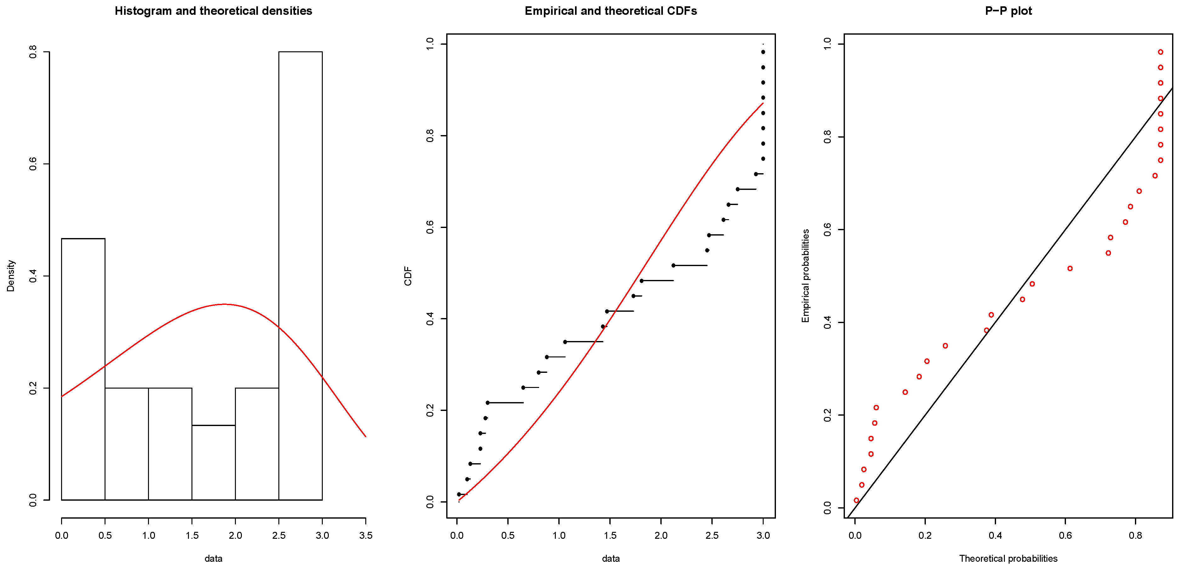
In this part, two real data sets were chosen for the illustration purpose of the proposed SkSP-R plan. To begin, we examine whether data sets have been fitted to the GmzD or not. To accomplish this purpose, several criteria such as Akaike information criterion (AIC), Bayesian information criterion (BIC), and Kolmogorov–Smirnov statistic (KS) goodness-of-fit test value were used. Moreover, the p-value associated with the KS test were considered to support the presented results based on the real data sets. Descriptive statistics summary and model fitting results of both data sets are presented in

Table 5. Descriptive summary of data sets.

Data	Minimum	${\mathit{Q}}_1$	Median	Mean	${\mathit{Q}}_3$	Maximum	CS	CK
I	0.020	0.688	1.965	1.770	2.983	3.000	−0.2840467	1.453664
II	0.550	1.375	1.590	1.507	1.685	2.240	−0.8999263	3.923761

and

Table 6. Measures of goodness-of-fit statistics for both data sets.

Data	Estimates	L-L	AIC	BIC	KS Value	p-Value
I	$\alpha =1.3509349,\theta =0.2496109$	$-41.34595$	$86.6919$	$89.4943$	$0.18892$	$0.2346$
II	$\alpha =0.2741801,\theta =0.0024180$	$-14.80810$	$33.61621$	$37.90247$	$0.12676$	$0.2635$

, respectively.

Data I: The data include 30 observations of the times of failures and running times for samples of devices from an eld-tracking study of a larger system. Previously, these data were studied by [32]. The data are as follows: 0.02, 0.10, 0.13, 0.23, 0.23, 0.28, 0.30, 0.65, 0.80, 0.88, 1.06, 1.43, 1.47, 1.73, 1.81, 2.12, 2.45, 2.47, 2.61, 2.66, 2.75, 2.93, 3.00, 3.00, 3.00, 3.00, 3.00, 3.00, 3.00, and 3.00. Figure 3 shows the histogram density, empirical CDF and P-P plot of the GmzD for the first data set.

The estimated parameters $\alpha$ and $\theta$ values are $1.3509349$ and $0.2496109$, respectively, based on Data I. Suppose that a researcher likes to set the mean life ${\mu }_0$ as $0.4$ unit and termination ratio $t_0/{\mu }_0$ = $0.5$; then, based on these values, termination time $t_0$ is $0.2$. For the considered setup, $\alpha =1.3509349,t_0/{\mu }_0=0.5$, $\beta =0.25$, and ${\alpha }_p=0.05$; the plan parameters of suggested SkSP-R plan are $(n=28,c=5,i=2,f=0.5,k=1,m=2)$; and the process is described follows:

1.

Start normal inspection and put $n=28$ items on test for prefixed time $t_0=0.2$. Detect and count the number of sample items that failed before the experiment duration, say, $d=3$, and $d\le 5$. Hence, accept the lot.

2.

When $i=2$, consecutive lots are not rejected under normal inspection based on time truncated life test; end the normal inspection and follow SI.

3.

Throughout SI, test only a fraction $f=0.5$ of lots chosen at random. SI is continued up to a point where a sampled lot is rejected.

4.

After $k=1$, where a lot is rejected, consecutively sampled lots are accepted; hence, utilize the resampling method for the immediate next lot as in Step 5.

5.

In the resampling technique, perform the inspection based on a reference plan. If the lot is not rejected, then keep SI. If the lot is not accepted, resampling is formed for $m=2$ times and the lot is rejected if it is not accepted on $(m-1)=2-1$st resubmission.

6.

If a lot is not accepted on resampling scheme, then immediately proceed to the normal inspection provided in Step 1.

7.

Remove or correct all the nonconforming items found with asserting units in the rejected lots.

The ASN value is $22.65489$. When the quality ratio is $\mu /{\mu }_0=3$, the probability of acceptance of the lot is $0.9882626$.

Data II: The data set was obtained by [33]. It consists of 63 observations the strengths of $1.5$ cm glass fibers, measured by the National Physical Laboratory, England. The data include the following: 0.77, 0.81, 0.84, 0.93, 1.04, 0.55, 0.74, 1.11, 1.13, 1.24, 1.25, 1.27, 1.28, 1.29, 1.30, 1.36, 1.39, 1.42, 1.48, 1.52, 1.53, 1.54, 1.55, 1.55, 1.48, 1.49, 1.49, 1.50, 1.76, 1.76, 1.77, 1.78, 1.81, 1.82, 1.84, 1.50, 1.51, 1.73, 1.84, 1.89, 2.00, 1.58, 1.59, 1.60, 1.61, 1.61, 1.61, 1.68, 1.68, 1.69, 1.70, 1.70, 1.61, 1.62, 1.62, 1.63, 1.64, 1.66, 1.66, 1.66, 1.67, 2.01, and 2.24. Figure 4 illustrates the histogram density, empirical CDF and P-P plot of the GmzD for the second data set.

The estimated values of parameters $\alpha$ and $\theta$ are $0.2741801$ and $0.0024180$, respectively, for the Data II. Suppose that the researcher wants to set the mean life ${\mu }_0$ to be $1.2$ unit and termination ratio $t_0/{\mu }_0$ as $0.5$; then, by using this information, termination time $t_0$ is $0.6$. For the considered setup, $\alpha =0.2741801,t_0/{\mu }_0=0.5$, $\beta =0.25,{\alpha }_p=0.05$, and the plan parameters of proposed SkSP-R plan are $(n=54,c=1,i=2,f=0.5,k=1,m=2)$; moreover, the process is as follows:

1.

Start normal inspection and put $n=54$ items on the test for prefixed time $t_0=0.6$. Detect and count the number of sample items which failed before the experiment duration, say, $d=1$, and $d\le 1$. Thus, we accept the lot.

2.

When $i=2$, consecutive lots are accepted under normal inspection based on time truncated life test, and the normal inspection is discontinued. A switch to the skipping inspection is made.

3.

During the skipping inspection, inspect only a fraction $f=0.5$ of lots selected at random. The skipping inspection is continued until a sampled lot is rejected.

4.

If the lot is rejected after $k=1$, consecutively sampled lots are accepted; then, proceed to the resampling procedure for the immediate next lot as in Step 5 provided below.

5.

During resampling procedure, perform the inspection using the reference plan. If the lot is accepted, then continue the skipping inspection. Upon the non-acceptance of the lot, resampling is performed for $m=2$ times and the lot is rejected if it has not been accepted on $(m-1)=2-1$st resubmission.

6.

If a lot is rejected on resampling scheme, then immediately revert to the normal inspection in Step 1.

7.

Remove or correct all nonconforming units found with conforming units in the rejected lots.

The ASN value is $43.26171$. When the quality ratio is $\mu /{\mu }_0=3$, then probability of acceptance of lot is $0.9676758$.

The above explained real life examples show the superiority of the proposed SkSP-R plan and how one can use it in real life situations.

6. Conclusions

The purpose of this paper is to develop a new SkSP-R for GmzD. We have discussed the GmzD characteristics with mean properties. The SkSP-R design for GmzD is presented in this study along with an optimization problem that aids in determining the suggested SkSP-R plan parameters. The necessary tables of the proposed plan are provided and discussed for various values of the distribution parameter $\theta$. Two real life examples were used to support the suggested SkSP-R plan’s applicability in real life scenarios. It turned out that industrialists or engineers can use the proffered tables to control the quality of the product. The results in this paper can be modefied based on ranked set sampling method as a future work [34,35,36].

References

- Gupta, S.S.; Groll, P.A. Gamma distribution in acceptance sampling based on life test. J. Am. Stat. Assoc. 1961, 56, 942–970. [Google Scholar] [CrossRef]
- Gupta, S.S. Life test sampling plans for normal and lognormal distributions. Technometrics 1962, 4, 151–175. [Google Scholar] [CrossRef]
- Baklizi, A.; EL Masri, A.E.K. Acceptance sampling plan based on truncated life tests in the Birnbaum Saunders model. Risk Anal. 2004, 24, 1453–1457. [Google Scholar] [CrossRef] [PubMed]
- Rosaiah, K.; Kantam, R.R.L. Acceptance sampling plan based on the inverse Rayleigh distribution. Econ. Qual. Control 2005, 20, 77–286. [Google Scholar] [CrossRef]
- Tsai, T.R.; Wu, S.J. Acceptance sampling plan based on truncated life tests for generalized Rayleigh distribution. J. Appl. Stat. 2006, 33, 595–600. [Google Scholar] [CrossRef]
- Balakrishnan, N.; Lieiva, V.; Lopez, J. Acceptance sampling plan from truncated life tests based on generalized Birnbaum Saunders distribution. Commun. Stat.-Simul. Comput. 2007, 34, 799–809. [Google Scholar] [CrossRef]
- Aslam, M.; Kundu, D.; Ahmed, M. Time truncated acceptance sampling plans for generalized exponential distribution. J. Appl. Stat. 2010, 37, 555–566. [Google Scholar] [CrossRef]
- Al-Omari, A.I. Time truncated acceptance sampling plans for generalized inverted exponential distribution. Electron. J. Appl. Stat. Anal. 2015, 8, 1–12. [Google Scholar]
- Tripathi, H.; Saha, M.; Alha, V. An application of time truncated single acceptance sampling inspection plan based on generalized half-normal distribution. Ann. Data Sci. 2020. [Google Scholar] [CrossRef]
- Saha, M.; Tripathi, H.; Dey, S. Single and double acceptance sampling plans for truncated life tests based on transmuted Rayleigh distribution. J. Ind. Prod. Eng. 2021, 38, 356–368. [Google Scholar] [CrossRef]
- Govindaraju, K.; Lai, C.D. A modified ChSP-1 chain sampling plan, MChSP-1,with very small sample sizes. Am. J. Math. Manag. Sci. 1998, 18, 343–358. [Google Scholar] [CrossRef]
- Govindaraju, K.; Subramani, K. Selection of chain sampling plans ChSP-1 and ChSP-(0,1) for given acceptable quality level and limiting quality level. Am. J. Math. Manag. Sci. 1993, 13, 123–136. [Google Scholar]
- Rao, G.S. Double acceptance sampling plan based on truncated life tests for Marshall-Olkin Extended exponential distribution. Austrian J. Stat. 2011, 40, 169–176. [Google Scholar] [CrossRef]
- Rao, G.S. A Group Acceptance Sampling Plans for Lifetimes Following a Marshall-Olkin Extended Exponential Distribution. Appl. Appl. Math. Int. J. 2011, 6, 592–601. [Google Scholar]
- Gui, W. Double acceptance sampling plan for truncated life tests based on Maxwell distribution. Am. J. Math. Manag. Sci. 2014, 33, 98–109. [Google Scholar] [CrossRef]
- Gui, W.; Xu, M. Double acceptance sampling plan based on truncated life tests for half exponential power distribution. Stat. Methodol. 2015, 27, 123–131. [Google Scholar] [CrossRef]
- Al-Omari, A.I.; Amjad, D.; Fatima, S.G. Double acceptance sampling Plan for time-truncated life tests based on half-normal distribution. Econ. Qual. Control. 2016, 31, 93–99. [Google Scholar]
- Al-Omari, A.I. Acceptance sampling plans based on truncated life tests for Sushila distribution. J. Math. Fundam. Sci. 2018, 50, 72–83. [Google Scholar] [CrossRef] [Green Version]
- Al-Omari, A.I.; Zamanzade, E. Double Acceptance Sampling Plan for time truncated life Tests based on transmuted generalized inverse weibull distribution. J. Stat. Appl. Probab. 2017, 6, 1–6. [Google Scholar] [CrossRef]
- Hu, M.; Gui, W. Acceptance sampling plans based on truncated life tests for Burr type X distribution. J. Stat. Manag. Syst. 2018, 21, 323–336. [Google Scholar] [CrossRef]
- Aslam, M.; Jun, C.H.; Ahmad, M. A Group sampling plan based on truncated life test for gamma distributed items. Pak. J. Stat. 2009, 25, 333–340. [Google Scholar]
- Aslam, M.; Jun, C.H.; Ahmad, M. New acceptance sampling plans based on life tests for Birnbaum–Saunders distribution. J. Appl. Stat. 2011, 81, 461–470. [Google Scholar] [CrossRef]
- Aslam, M.; Azam, M.; Lio, Y.; Jun, C.H. Two-Stage group acceptance sampling plan for Burr type X percentiles. J. Test. Eval. 2013, 41, 525–533. [Google Scholar] [CrossRef]
- Singh, S.; Tripathi, Y.M. Acceptance sampling plans for inverse Weibull distribution based on truncated life test. Life Cycle Reliab. Saf. Eng. 2017, 6, 169–178. [Google Scholar] [CrossRef] [Green Version]
- Kanaparthi, R.; Rao, G.S.; Kalyani, K.; Sivakumar, D.C.U. Group acceptance sampling plans for lifetimes following an odds exponential log logistic distribution. Sri Lankan J. Appl. Stat. 2016, 17, 201–216. [Google Scholar] [CrossRef] [Green Version]
- Tripathi, H.; Al-Omari, A.I.; Saha, M.; Mali, A. Time truncated life tests for new attribute sampling inspection plan and its applications. J. Ind. Prod. Eng. 2021b, 293–305. [CrossRef]
- Tripathi, H.; Al-Omari, A.I.; Saha, M.; Alanzi, A.R. Improved attribute chain sampling plan for Darna distribution. Comput. Syst. Sci. Eng. 2021, 38, 381–392. [Google Scholar] [CrossRef]
- Tripathi, H.; Saha, M.; Dey, S. A new approach of time truncated chain sampling inspection plan and its applications. Int. J. Syst. Assur. Eng. Manag. 2022. [Google Scholar] [CrossRef]
- Tripathi, H.; Dey, S.; Saha, M. Double and group acceptance sampling plan for truncated life test based on inverse log-logistic distribution. J. Appl. Stat. 2021, 48, 1227–1242. [Google Scholar] [CrossRef]
- Balamurali, S.; Aslam, M.; Jun, C.-H. A new system of skip-lot sampling including resampling. Sci. World J. 2014, 2014, 192412. [Google Scholar] [CrossRef]
- Balamurali, S.; Usha, M. Optimal designing of variables chain sampling plan by minimizing the average sample number. Int. J. Manuf. Eng. 2013, 2013, 751807. [Google Scholar] [CrossRef]
- Meeker, W.Q.; Escobar, L.A. Statistical Methods for Reliability Data; John Wiley and Sons: Hoboken, NJ, USA, 1988. [Google Scholar]
- Smith, R.L.; Naylor, J.C. A Comparison of Maximum Likelihood and Bayesian Estimators for the Three-Parameter Weibull Distribution. J. R. Stat. Soc. Ser. C (Appl. Stat.) 1987, 36, 358–369. [Google Scholar] [CrossRef]
- Al-Nasser, D.A.; Al-Omari, A.I. MiniMax ranked set sampling. Rev. Investig. Oper. 2018, 39, 560–570. [Google Scholar]
- Zamanzade, E.; Al-Omari, A.I. New ranked set sampling for estimating the population mean and variance. Hacet. J. Math. Stat. 2016, 45, 1891–1905. [Google Scholar] [CrossRef]
- Haq, A.; Brown, J.; Moltchanova, E.; Al-Omari, A.I. Paired double ranked set sampling. Commun. Stat.-Theory Methods 2016, 45, 2873–2889. [Google Scholar] [CrossRef]
Figure 1.
Plots of pdf (a) and cdf (b) of the GmzD for various values of parameters.
Figure 2.
Plots of hazard rate (a) and reliability (b) functions of the GmzD for various values of parameters.
Figure 3.
Histogram density, empirical CDF and P-P plot of the GmzD for the first data set.
Figure 4.
Histogram density, empirical CDF and P-P plot of the GmzD for the second data set.