
Prediction of Suspended Sediment Concentration Based on the Turbidity-Concentration Relationship Determined via Underwater Image Analysis


Department of Hydro Science and Engineering Research, Korea Institute of Civil Engineering and Building Technology, Goyang 10285, Korea
*
Author to whom correspondence should be addressed.
Appl. Sci. 2022, 12(12), 6125; https://doi.org/10.3390/app12126125
Submission received: 10 May 2022
/
Revised: 9 June 2022
/
Accepted: 13 June 2022
/
Published: 16 June 2022
(This article belongs to the Special Issue Intelligent Approaches in Predicting Hydrodynamics and Sediment Transport)
Abstract
:Sediment measurement data are essential for sediment transport analysis and therefore highly important in overall river planning. Extant sediment measurement methods consume considerable manpower and time and are limited by factors including economic reasons and worker risks. This study primarily aimed to predict the changes in SSC (Suspended Sediment Concentration) and turbidity by examining the change in color in underwater images. While maintaining a constant flow in a channel, the turbidity and concentration were measured under different SSC. Multiple regression models were developed using turbidity measurement results, and they exhibited high explanatory powers (adjusted R2 > 0.91). Furthermore, upon verification using the verification dataset of the experimental results, an excellent predictive power (RMSE ≈ 0.4 NTU) was demonstrated. The model with the highest predictive power, which was inclusive of red and green bands and showed no underlying multicollinearity was used to predict turbidity. Finally, the turbidity and suspended sediment concentration relationship determined from the experimental results was used to estimate the sediment concentration from the color changes in the underwater images. The concentrations that were predicted by the model showed satisfactory results, compared to the measurements (RMSE ≈ 21 ppm). This study indicated the feasibility of continuous SSC monitoring using underwater images as a new measurement method.
1. Introduction
Various types of problems occur during sediment generation, transportation, and deposition. In particular, sediments cause serious problems in river maintenance, such as changes in the riverbed, water pollution, and a direct influence on the functions of hydraulic facilities [1,2]. Therefore, it is extremely important to quantitatively identify and predict the amount of sediment in order to realize eco-friendly and sustainable river development [3,4,5,6,7,8,9]. In South Korea, the sediment-related problems occur locally on a relatively small-scale, and most of the sediment is transported in the form of suspended matter during the flood season, unlike the continental regions [6,10]. Therefore, data on the amount of sediment that is measured at multiple points are required. However, it is challenging to add additional measurement points owing to economic reasons. In addition, sediment measurement during the flood season is extremely difficult, dangerous, and requires considerable manpower and time because of high flow velocities, thereby necessitating the introduction of a novel measurement method.
Theoretically, the total amount of sediment that is transported in a river is the total quantity of the sediment that passes through the cross section of the river, and it is generally measured via different methods by categorization into the suspended sediment and bed load [11]. The suspended sediment is measured using mechanical samplers, such as depth-integrating samplers (D-74) and point-integrating samplers (P-61), and bottle samplers are mainly used for water sampling. When discrete interval sampling is used for water sampling, the discontinuous measurements and high sampling cost hinder the capture of the dynamic processes of sediment transport, deposition, and resuspension under field conditions. To overcome these shortcomings, devices that are capable of on-site real-time measurements have been developed for suspended sediment concentration (SSC) monitoring [12,13]. The laser diffraction method can solve this time resolution problem, and many studies have been actively conducted since the late 1990s to analyze its applicability and validity [14]. Meral [15] evaluated the applicability of the acoustic backscatter system and optical laser diffraction instrument (LISST) for suspended sediment measurement through laboratory experiments. In addition, Gartner et al. [16] reported that the SSC and particle size distribution can be accurately measured within the measurement range of LISST, thus indicating the applicability of LISST for laboratory experiments and research in rivers. Traykovski et al. [17] performed laboratory experiments using natural sediment to compare the measurement results of LISST with the results of sieving, filtration, and weighting techniques that are conventional suspended sediment analysis methods. They verified that LISST presents the accurate particle size distribution of sediment. The accuracy and validity of the equipment have been verified through various studies. However, economic and technical problems are still encountered during field application.
There is a growing interest in the newly applied methods for the prediction of suspended sediment and understanding sediment characteristics from image analysis. In recent years, an increasing number of studies have been conducted to measure the SSC and analyze the characteristics of sediment using images. Ghorbani et al. [18] proposed a suspended sediment monitoring method that estimates the turbidity of suspended sediment using the machine-learning-based analysis of the images captured from the water surface and employs the turbidity-concentration relationship. Nonetheless, for images capturing the water surface in air, the technologies for signal separation and division need to be improved because the signals that are reflected from the water surface, water body, and bottom are mixed, and an accurate analysis is difficult because the reflection tendency varies depending on the riverbed material. This study entailed fundamental research on suspended sediment monitoring through underwater imaging and the development of a relatively safer and more economical method than the existing methods for suspended sediment measurement. Specifically, the difference in chromaticity values (RGB and gray scale) among three different concentrations was confirmed via underwater imaging by performing an experiment, and multiple linear regression models were developed to predict the turbidity based on the obtained values. The possibility of estimating the SSC from the predicted turbidity value using the turbidity-concentration relationship was subsequently confirmed.
2. Materials and Methods
2.1. Experimental Method
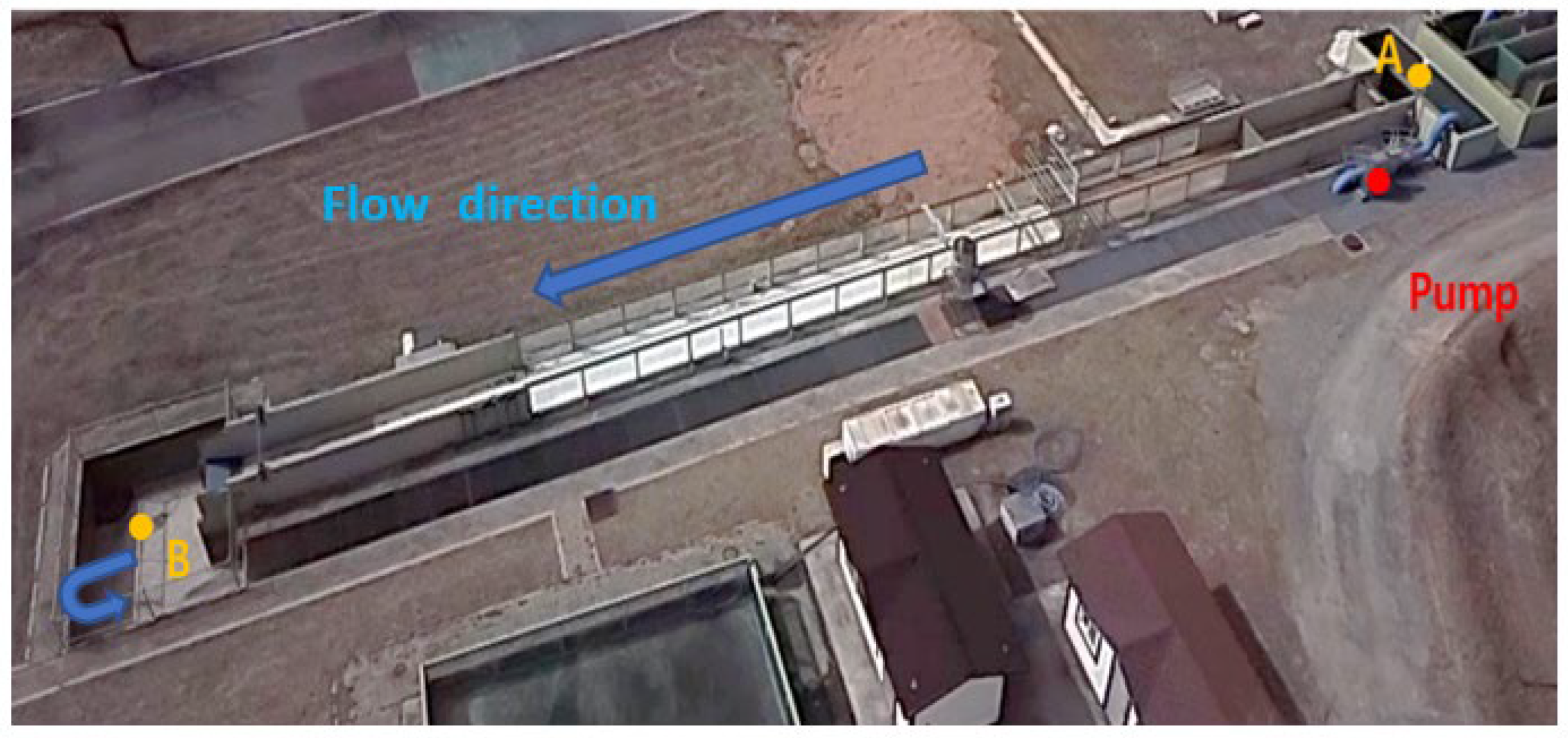
An experiment was performed in a 50 m long circulating channel in the Andong River Experiment Center (REC) of the Korea Institute of Civil Engineering and Building Technology (KICT) located in Andong, Gyeongsangbuk-do, Korea. Water flows in the direction from A to B in the channel, and the water at the end of the channel is circulated through a pump and supplied again to the channel (Figure 1).
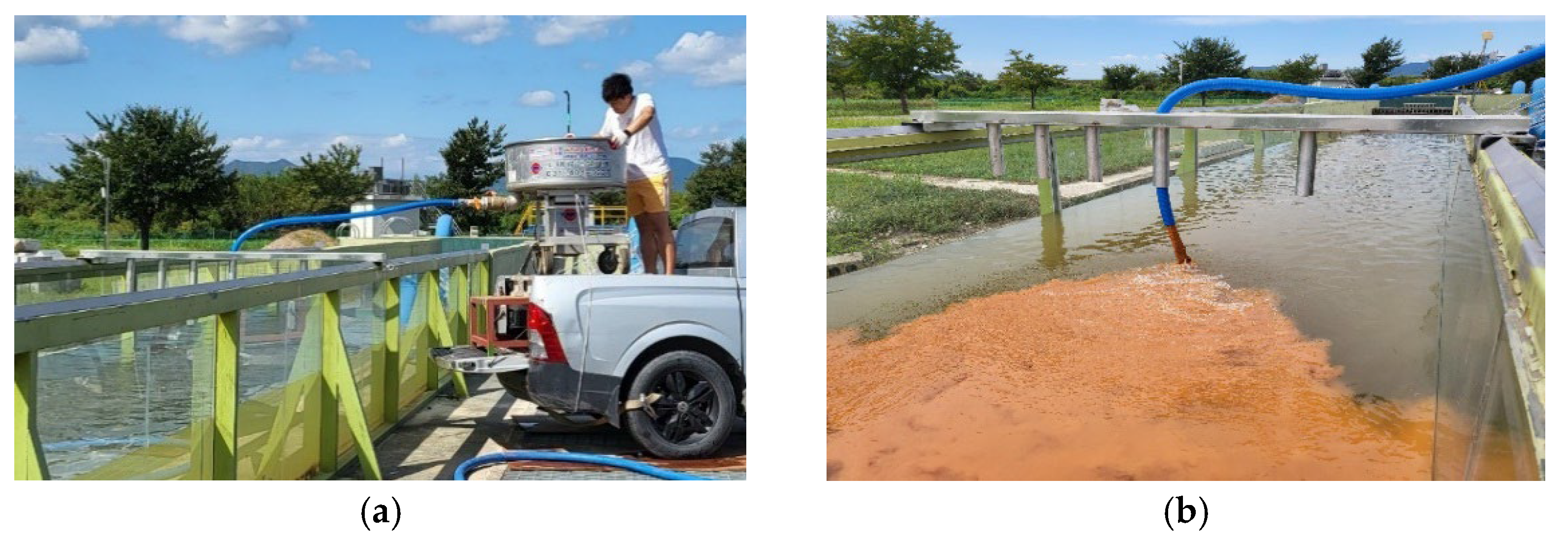
The channel has a width of 2 m and a height of 1.25 m. The necessary measurements were acquired in a section where temperature glass was installed, such that the equipment and experimental environment could be directly examined from the outside. The suspended sediment mixture was injected at the 22 m point of the circulating channel, and the measurement instruments for turbidity and concentration were located to take measurements at the 32 m point. The flow velocity and water depth were measured using a side-looking acoustic Doppler current profiler (ADCP-SL) and ADCP-M9 at 1 m upstream and downstream positions that were relative to the turbidity and SSC measurement position. Finally, two GoPro 9 units were installed upstream and downstream of the point where the sediment supply was performed (18 m, Video 1 and 31.8 m, Video 2). Red clay powder with a particle diameter smaller than 0.044 mm was used to examine the color change of water, according to the SSC. The powder and water were sufficiently mixed with 200 L of water using a 250 L mixer, and the mixture was injected for a certain period at the following three concentrations: (1) 1st Injection: 25 g/L (14:38:30–14:40:00); (2) 2nd Injection: 50 g/L (14:47:00–14:48:25); and (3) 3rd Injection: 75 g/L (15:04:00–15:05:05) (Figure 2).
The turbidity was measured at the center of the channel at a height of 38 cm from the floor using a multi-item water quality meter (WQC-30), and the SSC was measured using LISST-200X at the same point (Figure 3). In the case of turbidity and concentration measurements, there were unmeasured sections between the injections of the suspended sediment mixture of each condition. In the case of turbidity measurement using WQC-30, the 90° scattered light method, which measures the amount of light scattered at 90° by particles in water was used. The instrument was calibrated using the formazine standard solution, and measurements were performed every 2 s in the nephelometric turbidity units (NTU) [19]. LISST-200X measures the volumetric concentration based on particle size as the light source is scattered and calculates the laser light attenuation by suspended particles based on the transmittance of the unscattered laser light source. The particles in the 1.00–500 μm range could be measured, and measurements were performed every second for the total concentration of suspended sediment, particle size distribution, optical transmission, water depth, and water temperature [20].
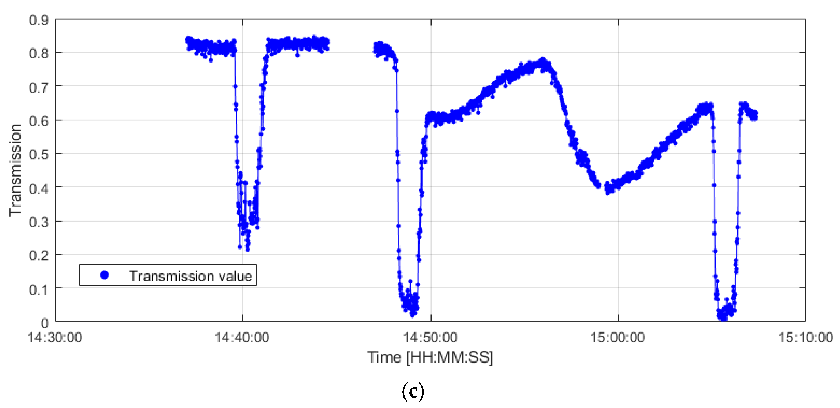
A total of 1642 SSCs and 828 turbidity measurements were captured; Figure 4 shows the turbidity, SSC, and transmission values that were measured throughout the experiment.
The instrument presents the transmission value as the risk of the ratio of multiple scattering for the evaluation the measurement results’ reliability (Figure 4c). Specifically, caution needs to be exercised against data quality degradation caused by many fine particles when the transmission value is less than 0.3; in fact, data may be neglected when the value is less than 0.1 [20]. The results indicated that the measured SSC during injection were not reliable. During the experiment, the pump continuously supplied at a flow rate of approximately 0.271 m3/s with 1600 RPM, and the flow velocity and water depth were measured to examine the stability of the flow rate (Figure 3b). With regard to the flow velocity, areas close to the sensor and the riverbed that could not be measured by ADCP-M9 were excluded, and the depth-averaged results are shown in Figure 5.
Velasco and Huhta [21] reported that the measurement accuracy of ADCP decreases in case of flow with a large amount of sediment. During the experiment of this study, outliers were also observed in the measurement results when high-concentration sediment was supplied. Even when such outliers (with deviations more than three times the standard deviation) were included, it was confirmed that the flow rate remained constant during the experiment as the flow velocity exhibited an average of 0.198 m/s and a standard deviation of 0.0088 m/s, and the water depth exhibited an average of 0.707 m and a standard deviation of 0.003 m.
2.2. Analysis Method
To compare and analyze color changes due to variations in the SSC and turbidity, images in 3840 2160 pixels were extracted every second from the continuously captured underwater images. From these images, RGB values and gray scale values were obtained (Equation (1)). RGB values are the three primary colors of light that are most commonly used to process the colors of digital images and can express intuitive and natural color space; gray scale values can express colors in gray by weighting and averaging the RGB values.
As the RGB values are different for each pixel even in the same image, an analysis was conducted for the following nine pixels among a total of 3840 2160 pixels: (1) [1000, 250]; (2) [1000, 1000]; (3) [1000, 1700]; (4) [1970, 250]; (5) [1970, 1000]; (6) [1970, 1700]; (7) [3000, 250]; (8) [3000, 1000]; and (9) [3000, 1700]. A multiple linear regression analysis was used to develop models, in order to predict turbidity from the chromaticity values that were obtained at the coordinates. The multiple linear regression equation for analyzing the relationship between the dependent variable and two or more independent variables is expressed in the form of Equation (2).
In this study, impure data and corresponding results (LISST equipment transmission value less than 0.3) were excluded during model development. In addition, the possibility of monitoring the SSC from underwater images using the turbidity-concentration relationship obtained from the measurement results was examined. Turbidity has been widely used instead of SSC measurement because it is affected by suspended and colloidal substances, such as clay, fine sand, plankton, and organic and inorganic substances, and continuous monitoring is possible owing to the relatively easy installation of equipment [22]. In general, empirical relationships are used to estimate the concentration from the turbidity. Because the turbidity-concentration relationship varies depending on the sediment particles, water characteristics, and measurement site, different relationships for each measurement site were proposed [23,24]. Because there is no formal conversion method for the turbidity-concentration relationship, the following three relationships are commonly used.
- (1)
- (2)
- (3)
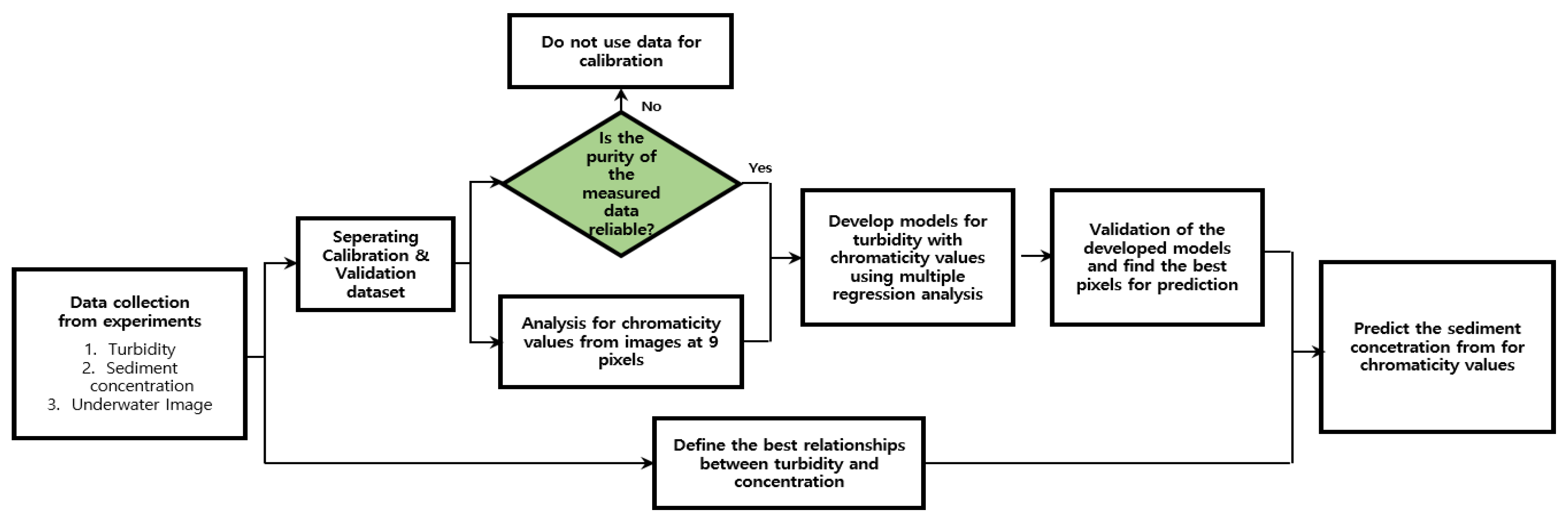
A flowchart of the entire process in this study is given in Figure 6.
3. Results
3.1. Measurement Results (RGB Values)
The underwater images that were captured by Video 2 clearly show the color changes resulting from the variations in SSC and turbidity (Figure 7).
The RGB and gray scale values obtained at the designated nine pixels that were obtained from the images captured by Video 2 are shown in Figure 8. The analysis results confirmed that the value of the red band increased as the SSC and turbidity increased. The other bands demonstrated the opposite tendency. Moreover, color changes occurred owing to the changes in the SSC and turbidity, even though slight differences were observed at the time of injecting the sediment, depending on the pixel coordinates.
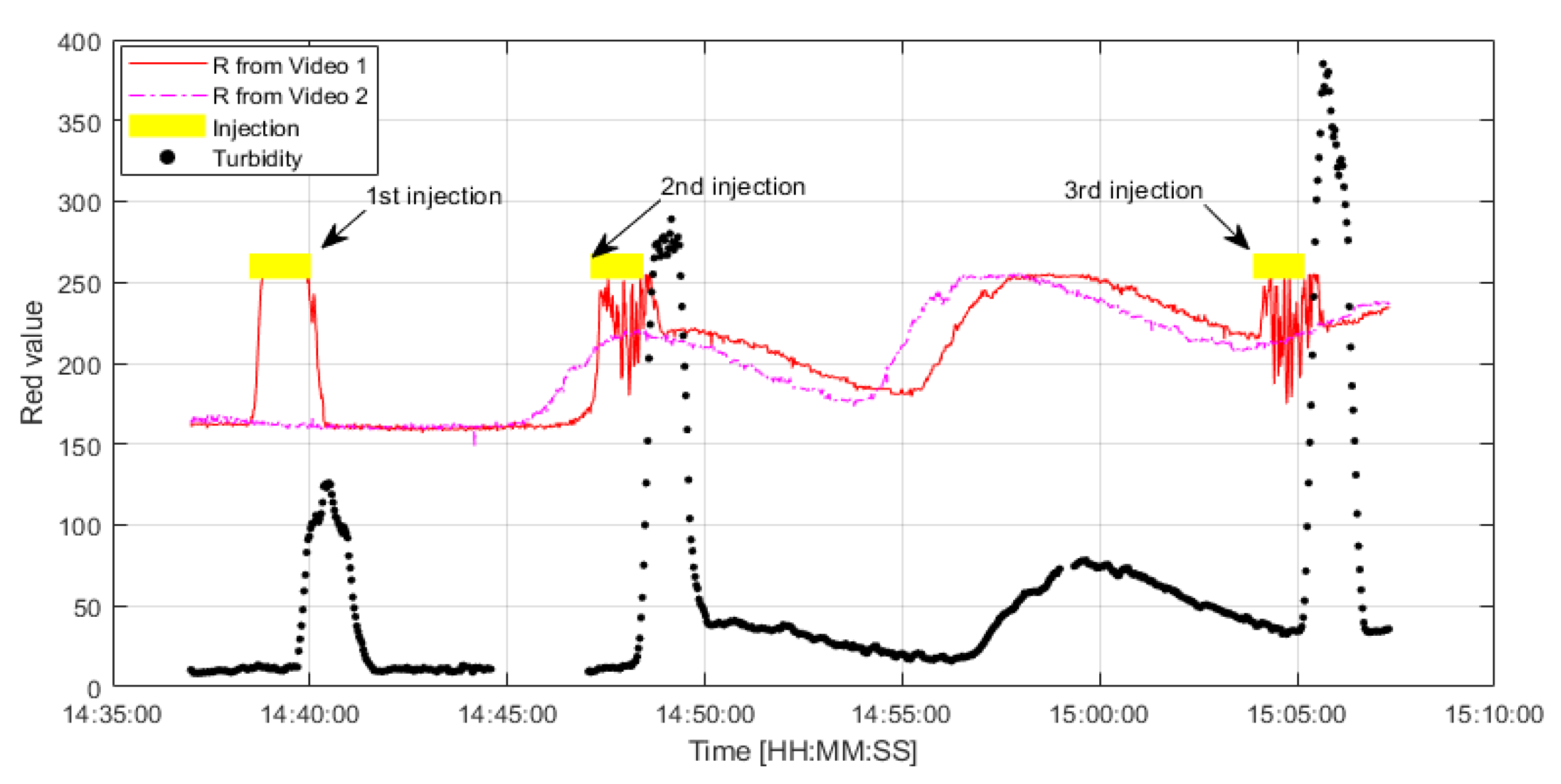
Considering the characteristics of the circulating channel where the flow was recirculated, the underwater images that were captured by Video 1 and Video 2 were compared; the comparison and analysis results of only the red band are presented in Figure 9.
When the RGB values of the images that were captured by Videos 1 and 2 were analyzed, it was found that the results of the 1st injection were captured immediately before the occurrence of the second injection (14:45:44), and the results of the second injection were captured at 14:54:18. In addition, it was found that changes in RGB values were directly affected by the suspended sediment injection results at the 10 m upstream position and RGB values severely fluctuated in the images that were captured during the injection of sediment, unlike the images of the recirculated sediment flow.
3.2. Model Development
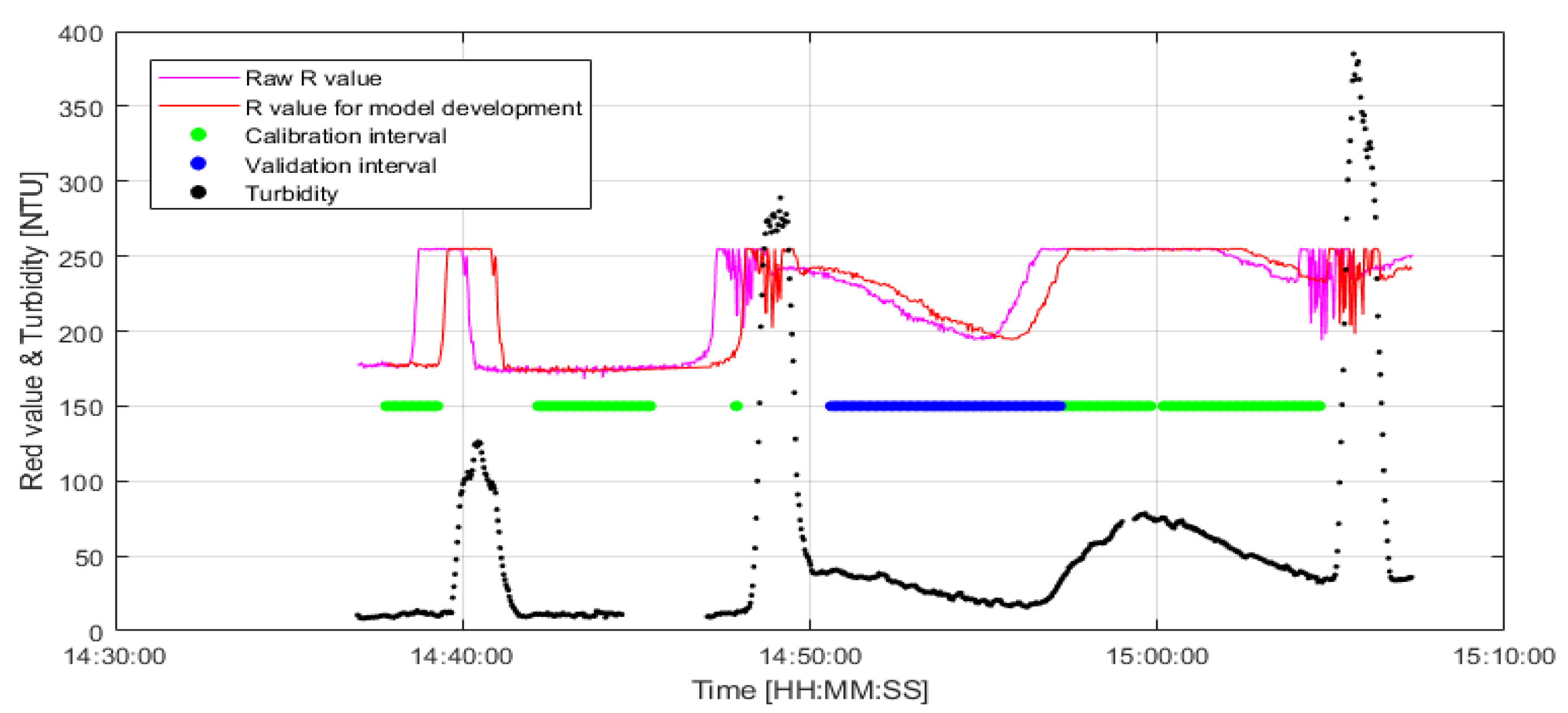
For the development of an accurate multiple regression model, the explanatory power of the independent variable for the dependent variables is extremely important. To develop a model for predicting turbidity from color changes in images, multiple regression equations were developed using a total of 502 data points, excluding low-reliability measurement results (LISST equipment transmission value less than 0.3), the data corresponding to RGB values severely fluctuating because of sediment injection, and the data that were reserved for verifying the developed regression equation (Figure 10).
Unlike turbidity and concentration measurements performed at a specific point and time, there was a time difference between the turbidity and concentration values that were measured at the same time and the RGB values that were analyzed from the images because the point of capture varied depending on the visibility range of the images. In this study, the model development was performed after reflecting the corresponding time difference on the dependent variable because the experiment was performed under a highly constant flow condition (average flow velocity = 0.198 m/s) and there was a constant time difference (50 s) between the occurrence of the change in red band value and an increase in turbidity (Figure 10). To develop a multiple linear regression model, regression models were developed using the five combinations of (R, G, B, Gray); (R, G, B); (R, G); (G, B); and (R, B) that were obtained from the nine pixels as independent variables with consideration of the time differences between the turbidity and explanatory variables. Table 1 shows the adjusted R-squared values.
Among the developed regression models, the models that included both RGB and the gray scale showed the highest values and the regression equations that included the red band generally presented high values. In addition, the regression models developed using the data obtained from the pixels that were parallel to the concentration and turbidity measuring instruments among the nine pixels generally showed high adjusted R-squared values (* in Table 1). The regression models that were developed based on the pixels are as follows:
For evaluating the developed regression models, the root mean squared error (RMSE) was calculated using the additional verification data using the following equation:
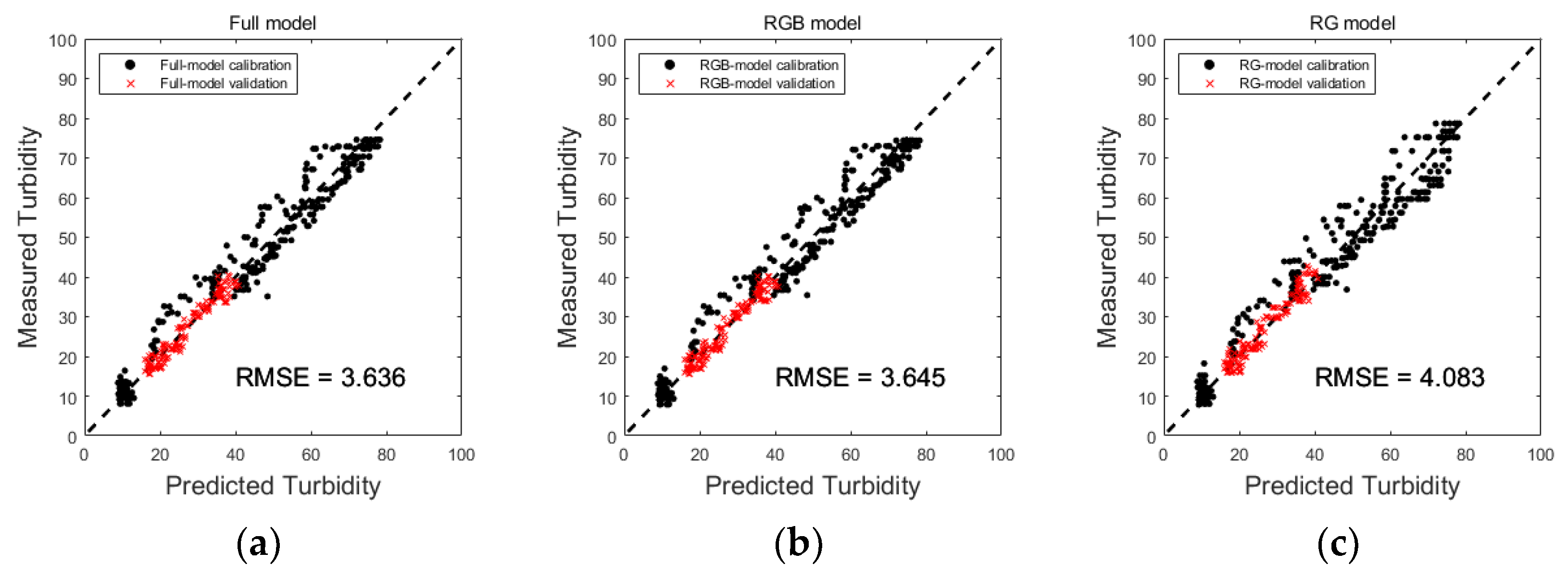
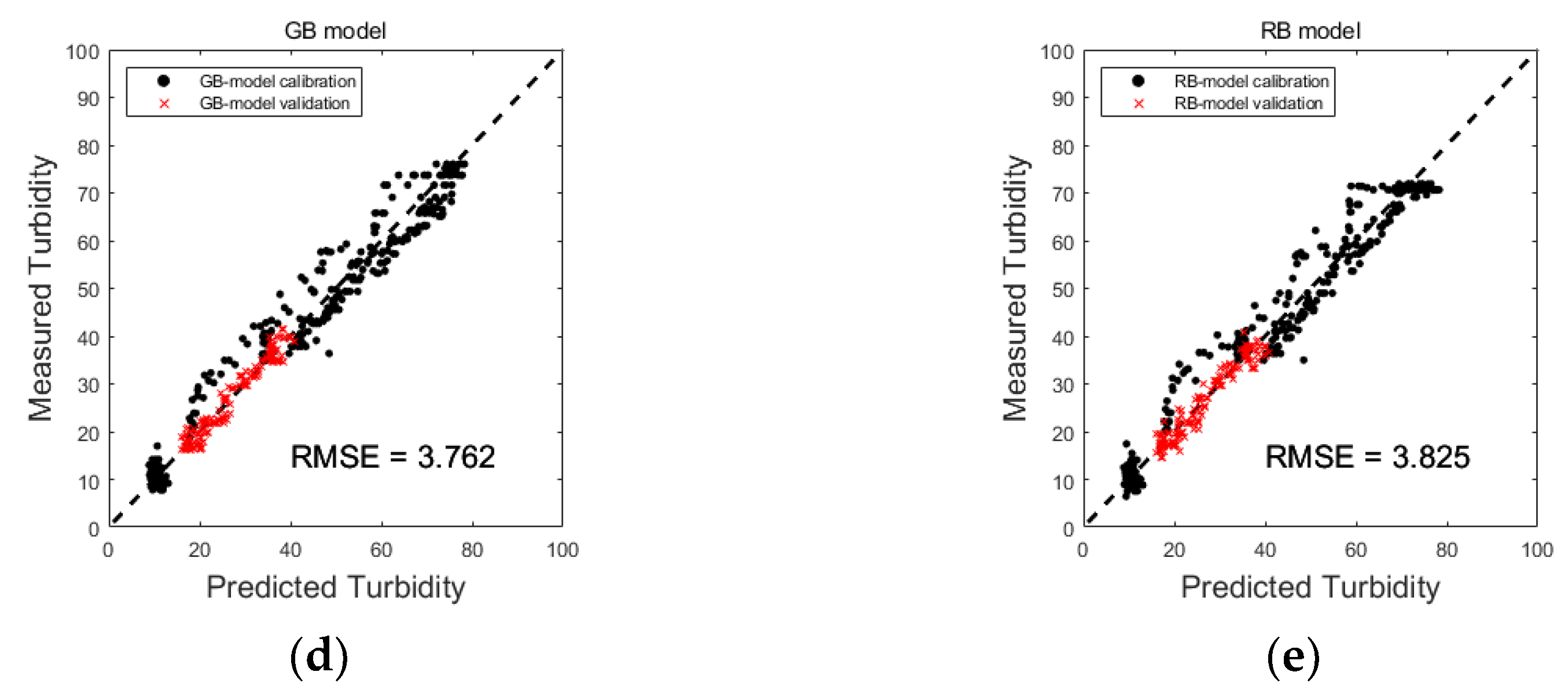
Figure 11 shows the results of verifying the five developed multiple regression models.
All the developed models showed the RMSE values of 3.6–4.1 NTU and presented highly satisfactory prediction results. In the case of multiple linear regression, correlations among the independent variables that cause an incorrect interpretation of variables or degrade the prediction accuracy need to be examined. In general, if the variance inflation factor (VIF) value is 10 or higher, the variables are judged to be multicollinear. VIF is calculated using Equation (9), and the results of examining multicollinearity are shown in Table 2.
The regression model that includes RGB and gray scale values showed extremely high multicollinearity. Among the developed models, the RG model (Equation (5)) and the GB model (Equation (6)) exhibit no multicollinearity. All the variables of the models exhibited high contribution to the regression model, with the p-value of the F-tests being 2 × 10⁻¹⁶ or less.
3.3. Estimation of Concentration from Turbidity
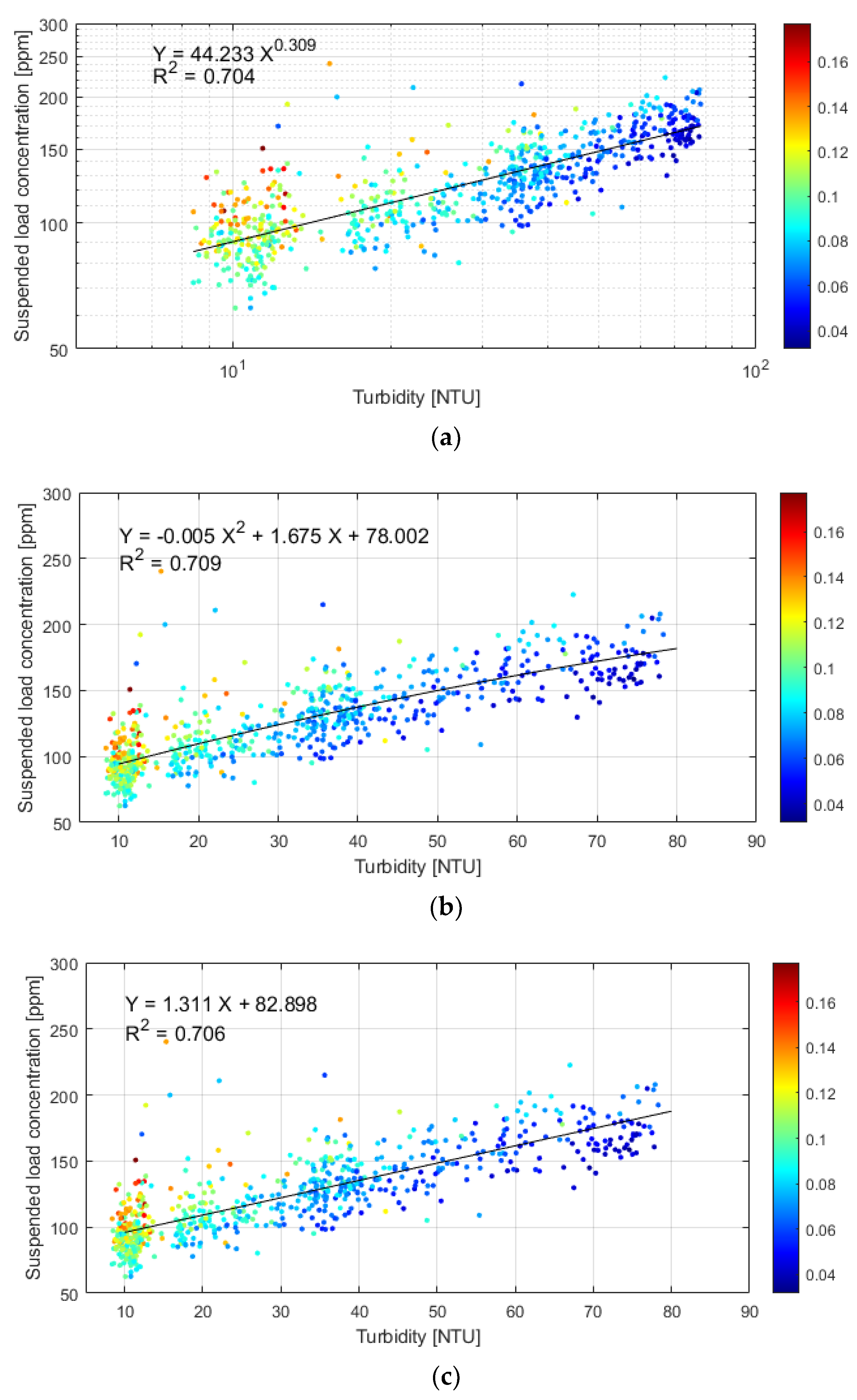
The turbidity-concentration relationship was analyzed from the data that were used for the model calibration and validation to estimate the concentration from the turbidity that was predicted using the developed models (Figure 12).
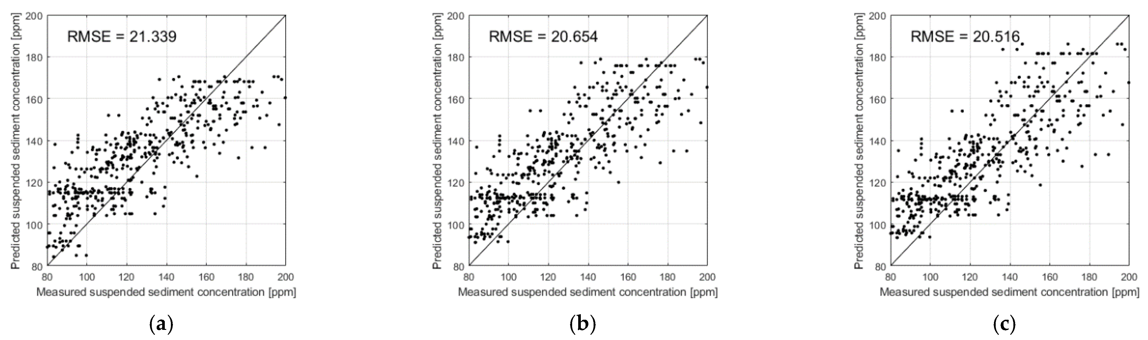
The proposed turbidity-concentration relationships showed similar R2 values. Considering that the size of the particles that were used for the suspended sediment injection was smaller than 0.044 mm, it was difficult to estimate the concentration from turbidity when the average particle size was increased by suspended substances other than the injected red clay. In particular, the section with low turbidity before suspended sediment injection exhibited a large deviation. Among the developed models, the RG model that showed the highest predictive power with no multicollinearity was used. Figure 13 shows the SSC that was estimated using the predicted turbidity by the model based on the presented turbidity-concentration relationship that is most commonly used (power-law).
In the case of the SSC that was estimated using the predicted turbidity by the developed model, the RMSE value ranged from 20 to 21 ppm, thus confirming the possibility of estimation of the SSC from color changes in images. In case of estimating the SSC based on this method, the predictive power is expected to further increase if larger amounts of data on SSC and turbidity are used.
4. Discussion
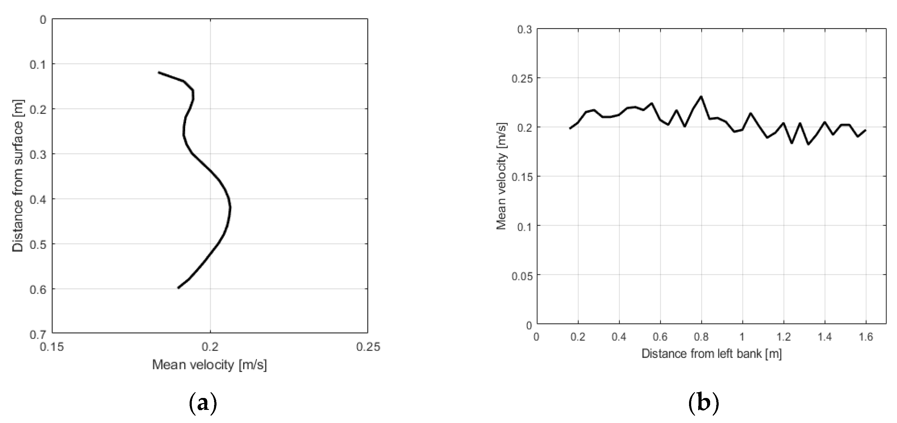
Figure 14 shows the vertical flow velocity distribution that was measured using ADCP-SL at the turbidity measurement position of 1 m upstream, and the horizontal flow velocity distribution that was measured using ADCP-M9 at the center of the channel 1 m downstream.
In the case of the mean velocity distribution in the vertical direction that was measured using ADCP, the section approximately 0.1 m from the water surface and the unmeasured section 0.1 m from the floor were excluded. It appears that the flow velocity decreased as the concentration and turbidity measuring instruments that were installed at 0.35 m from the floor at the upstream point 1 m from the flow velocity measurement point affected the flow. Except for this, the flow velocity distribution in a rectangular channel was observed. In the case of the horizontal flow velocity distribution, the highest flow velocity was observed at the center of the channel. Overall, a slightly higher flow velocity was observed on the left bank side because water was supplied by the pump that was located on the right side. When the vertical and horizontal distributions of the SSC were predicted from the color change of pixels in the images using the developed models, the SSC was found to increase as the water depth increased, and the conventional suspended sediment behavior with no significant difference in the horizontal direction was clearly observed (Figure 15).
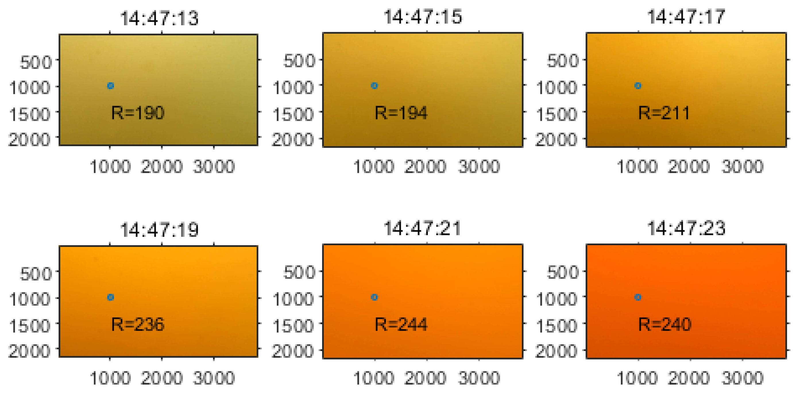
The proposed models showed excellent predictive power, but the data of the section where sediment was injected were not used for model development. This is because the RGB band values at the same pixel coordinates changed during the injection of sediment because of significant changes in brightness and saturation. In addition, it could be confirmed that blue or green colored water changed to red colored water because of the injection of sediment under the initial condition. However, there were limitations in estimating the slight color changes in red and orange using the RGB values alone (Figure 16).
To address such limitations, it is necessary to determine the conditions for river sediment imaging, such as appropriate camera exposure information and ISO values, through additional experiments; or to conduct further analysis on HSB (that is the combination of the hue, saturation, and brightness that is required to analyze the additional colors of light), or analysis on YCbCr models that separate the brightness component (Y) and color difference information (Cb and Cr) from the RGB colors for expression. In the case of the proposed method for estimating the SSC from color changes in images, it can be concluded that additional experiments and research are required for its actual application to rivers. First, while the experiment that was performed in this study used red clay that causes relatively clear color changes, additional experiments will be required for: (1) the suspended sediment condition that causes relatively small color changes in water (for example, sand); (2) the condition that considers particles with various particle size distributions at the same time; and (3) the condition without a constant flow. Considering the time difference between the turbidity and concentration measurement results and the images that were captured at the same time, image capturing in the direction that is perpendicular to the flow appears to be better than image capturing in the direction that is opposite to the flow. It is also deemed necessary to adjust the position of image capturing considering that RGB values severely fluctuate during the injection of sediment. In the future, additional experiments and research can be conducted using the information and various analysis methods presented above, including various image analysis methods, data analysis methods, and the method of measuring the SSC based on the ADCP backscatter intensity.
5. Conclusions
In this study, an experiment for estimating the SSC from color changes in underwater images was performed to develop a more economical and safer sediment measurement and monitoring method than the conventional methods. At a 32 m point, 828 turbidity data were captured every 2 s using WQC-30, and 1642 concentration data were captured every second using LISST in a 50 m circulating channel. Water mixed with red clay at three different concentrations (25, 50, and 75 gr/L) was injected for inducing color changes in underwater images according to the SSC, and the experiment was then conducted. Changes in the RGB and gray scale values were analyzed by extracting underwater images, and multiple linear regression models for turbidity prediction were developed using the results that were obtained from the images and turbidity measurement results. Using 502 data points, 45 models were developed for the five combinations of RGB and gray scale values at nine pixels that presented high predictive power for turbidity (adjusted R-squared > 0.91), and the models that were developed using the data obtained from the pixels corresponding to the turbidity measurement position particularly showed excellent predictive power. When the models were verified using the remaining 180 verification data points, they showed excellent RMSE values of approximately 4 NTU. Due to some models exhibiting multi-collinearity (VIF > 10), turbidity prediction was finally performed by applying the model incorporating red and green bands. In addition, three turbidity-concentration relationships were suggested using the data that were used for model development and verification. These relationships showed a similar explanatory power (R2 ≈ 0.7); however, they showed less correlations when the average particle size was large before the injection of the red clay mixture or when other suspended matter was mixed in large quantities. Finally, the concentration results that were predicted using the proposed turbidity model and the most commonly used turbidity-concentration relationship that were obtained from the experiment results showed satisfactory prediction results (RMSE ≈ 20 ppm), compared to the measured concentration results.
For the actual application of the proposed methodology, it is necessary to conduct additional experiments and research considering various experimental conditions and analysis methods. The experimental results, however, have confirmed that the SSC can be monitored from the color changes in underwater images if measurements are continuously performed at fixed points. Monitoring the SSC through underwater image processing is a promising technology, and some of the existing impediments to continuous sediment measurements for river management can be eliminated through additional research and experiments.
Author Contributions
Conceptualization, W.K.; formal analysis, W.K., K.L. and J.K.; writing—review and editing, W.K. All authors have read and agreed to the published version of the manuscript.
Funding
This research was supported by the National Research Foundation of Korea (NRF) grant funded by the Korea government (No. 2021R1C1C101040411).
Institutional Review Board Statement
Not applicable.
Informed Consent Statement
Not applicable.
Data Availability Statement
Not applicable.
Acknowledgments
This work utilized an experimental infrastructure at the River Experiment Center of the Korea Institute of Civil Engineering and Building Technology. This research was supported by ‘National Research Council of Science & Technology (NST)’-‘KOREA INSTITUTE of CIVIL ENGINEERING and BUILDING TECHNOLOGY (KICT)’ Postdoctoral Fellowship Program for Young Scientists at KICT in South Korea.
Conflicts of Interest
The authors declare no conflict of interest.
References
- Yoon, B.; Woo, H. Sediment problems in Korea. J. Hydraul. Eng. 2000, 126, 486–491. [Google Scholar] [CrossRef]
- Jolicoeur, S.; Caissie, D.; Frenette, I.; Hardie, P.; Bouchard, M. Suspended sediment concentration in relation to forestry operations in Catamaran Brook and its tributaries (Canada). River Res. Appl. 2006, 23, 141–154. [Google Scholar] [CrossRef]
- Kang, W.; Yang, C.Y.; Lee, J.; Julien, P.Y. Sediment yield for ungauged watersheds in South Korea. KSCE J. Civ. Eng. 2019, 23, 5109–5120. [Google Scholar] [CrossRef]
- Areu-Rangel, O.S.; Bonasia, R.; Di Traglia, F.; Del Soldato, M.; Casagli, N. Flood Susceptibility and Sediment Transport Analysis of Stromboli Island after the 3 July 2019 Paroxysmal Explosion. Sustainability 2020, 12, 3268. [Google Scholar] [CrossRef] [Green Version]
- Kang, W.; Jang, E.K.; Yang, C.Y.; Julien, P.Y. Geospatial analysis and model development for specific degradation in South Korea using model tree data mining. CATENA 2021, 200, 105142. [Google Scholar] [CrossRef]
- Kang, W.; Lee, K.; Jang, E.K. Evaluation and Validation of Estimated Sediment Yield and Transport Model Developed with Model Tree Technique. Appl. Sci. 2022, 12, 1119. [Google Scholar] [CrossRef]
- Wang, F.; Huai, W.; Guo, Y. Analytical model for the suspended sediment concentration in the ice-covered alluvial channels. J. Hydrol. 2021, 597, 126338. [Google Scholar] [CrossRef]
- Chassiot, L.; Lajeunesse, P.; Bernier, J.F. Riverbank erosion in cold environments: Review and outlook. Earth-Sci. Rev. 2020, 207, 103231. [Google Scholar] [CrossRef]
- John, C.K.; Pu, J.H.; Pandey, M.; Hanmaiahgari, P.R. Sediment deposition within rainwater: Case study comparison of four different sites in Ikorodu, Nigeria. Fluids 2021, 6, 124. [Google Scholar] [CrossRef]
- Yang, C.Y.; Kang, W.; Lee, J.H.; Julien, P.Y. Sediment regimes in South Korea. River Res. Appl. 2022, 38, 209–221. [Google Scholar] [CrossRef]
- Julien, P.Y. Erosion and Sedimentation, 2nd ed.; Cambridge University Press: Cambridge, UK, 2010. [Google Scholar]
- Gray, J.R.; Gartner, J.W. Technological advances in suspended-sediment surrogate monitoring. Water Resour. Res. 2009, 45. [Google Scholar] [CrossRef] [Green Version]
- Felix, D.; Albayrak, I.; Boes, R.M. Laboratory investigation on measuring suspended sediment by portable laser diffractometer (LISST) focusing on particle shape. Geo-Mar. Lett. 2013, 33, 485–498. [Google Scholar] [CrossRef] [Green Version]
- Wren, D.G.; Barkdoll, B.D.; Kuhnle, R.A.; Derrow, R.W. Field techniques for suspended-sediment measurement. J. Hydraul. Eng. 2000, 126, 97–104. [Google Scholar] [CrossRef]
- Meral, R. Laboratory evaluation of acoustic backscatter and LISST methods for measurements of suspended sediments. Sensors 2008, 8, 979–993. [Google Scholar] [CrossRef] [Green Version]
- Gartner, J.W.; Cheng, R.T.; Wang, P.F.; Richter, K. Laboratory and field evaluations of the LISST-100 instrument for suspended particle size determinations. Mar. Geol. 2001, 175, 199–219. [Google Scholar] [CrossRef]
- Traykovski, P.; Latter, R.J.; Irish, J.D. A laboratory evaluation of the laser in situ scattering and transmissometery instrument using natural sediments. Mar. Geol. 1999, 159, 355–367. [Google Scholar] [CrossRef]
- Ghorbani, M.A.; Khatibi, R.; Singh, V.P.; Kahya, E.; Ruskeepää, H.; Saggi, M.K.; Sivakumar, B.; Kim, S.; Salmasi, F.; Kashani, M.H.; et al. Continuous monitoring of suspended sediment concentrations using image analytics and deriving inherent correlations by machine learning. Sci. Rep. 2020, 10, 8589. [Google Scholar] [CrossRef]
- DKKTOA. Handheld Multi-Parameter Water Quality Meter Model WQC-30. Available online: http://www.sequoiasci.com/product/lisst-200x/ (accessed on 10 February 2021).
- Sequoia Scientific, Inc. LISST-200X Measures Particle Size Distribution and Concentration, and Optical VSF. Available online: https://www.toadkk.com/english/product/details/por/wqc-30.html (accessed on 20 January 2022).
- Velasco, D.W.; Huhta, C.A. Experimental verification of acoustic Doppler velocimeter (ADV) performance in fine-grained, high sediment concentration fluids. App Note SonTek/YSI 2010, 1–19. Available online: https://www.xylemanalytics.kr/media/pdfs/sontek-adv-in-fluid-mud.pdf (accessed on 1 February 2022).
- Bright, C.E.; Mager, S.M. A national-scale study of spatial variability in the relationship between turbidity and suspended sediment concentration and sediment properties. River Res. Appl. 2020, 36, 1449–1459. [Google Scholar] [CrossRef]
- Minella, J.P.; Merten, G.H.; Reichert, J.M.; Clarke, R.T. Estimating suspended sediment concentrations from turbidity measurements and the calibration problem. Hydrol. Process. 2008, 22, 1819–1830. [Google Scholar] [CrossRef] [Green Version]
- Rutherfurd, I.D.; Kenyon, C.; Thoms, M.; Grove, J.; Turnbull, J.; Davies, P.; Lawrence, S. Human impacts on suspended sediment and turbidity in the River Murray, South Eastern Australia: Multiple lines of evidence. River Res. Appl. 2020, 36, 522–541. [Google Scholar] [CrossRef]
Figure 1.
Experiment site: 50 m long circulating channel at the Andong River Experiment Center (REC).
Figure 1.
Experiment site: 50 m long circulating channel at the Andong River Experiment Center (REC).

Figure 2.
(a) Injection of red clay mixture using a 250 L mixer; (b) mixture injection method for Injection 3.
Figure 2.
(a) Injection of red clay mixture using a 250 L mixer; (b) mixture injection method for Injection 3.

Figure 3.
Measuring instruments used in the experiment: (a) WQC-30, LISST-200x, and GoPro 9 (Video-2 at 31.8 m), and (b) ADCP.
Figure 3.
Measuring instruments used in the experiment: (a) WQC-30, LISST-200x, and GoPro 9 (Video-2 at 31.8 m), and (b) ADCP.
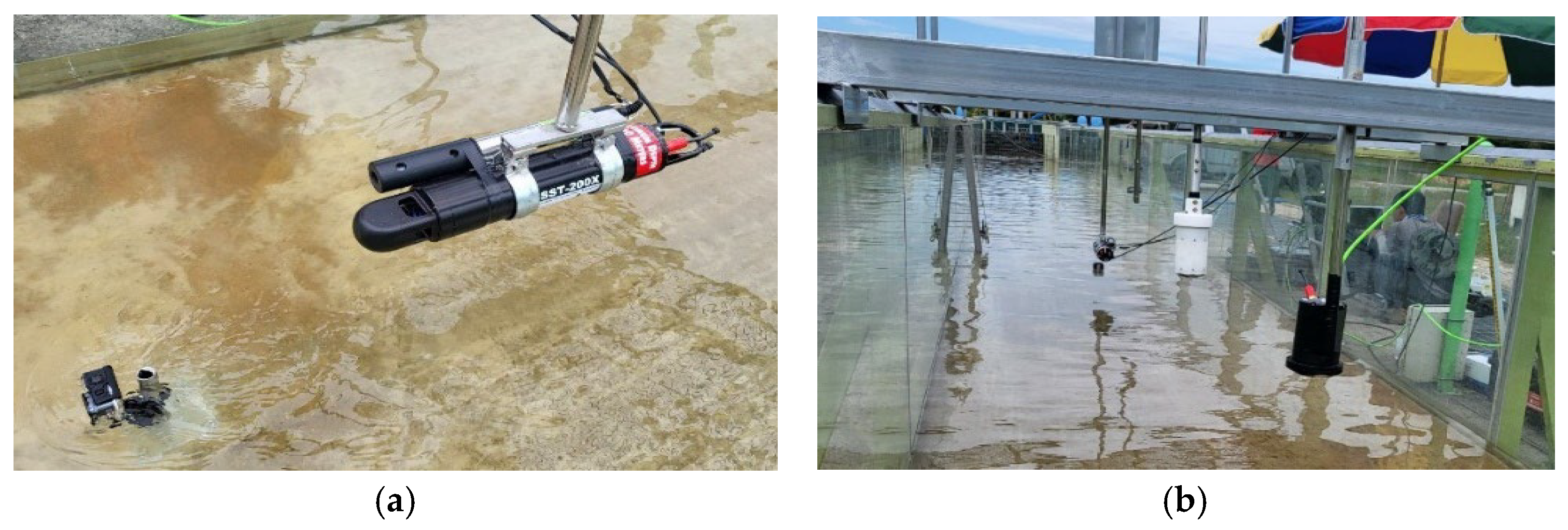
Figure 4.
Measurement results: (a) turbidity, (b) suspended sediment concentration, and (c) transmission value.
Figure 4.
Measurement results: (a) turbidity, (b) suspended sediment concentration, and (c) transmission value.
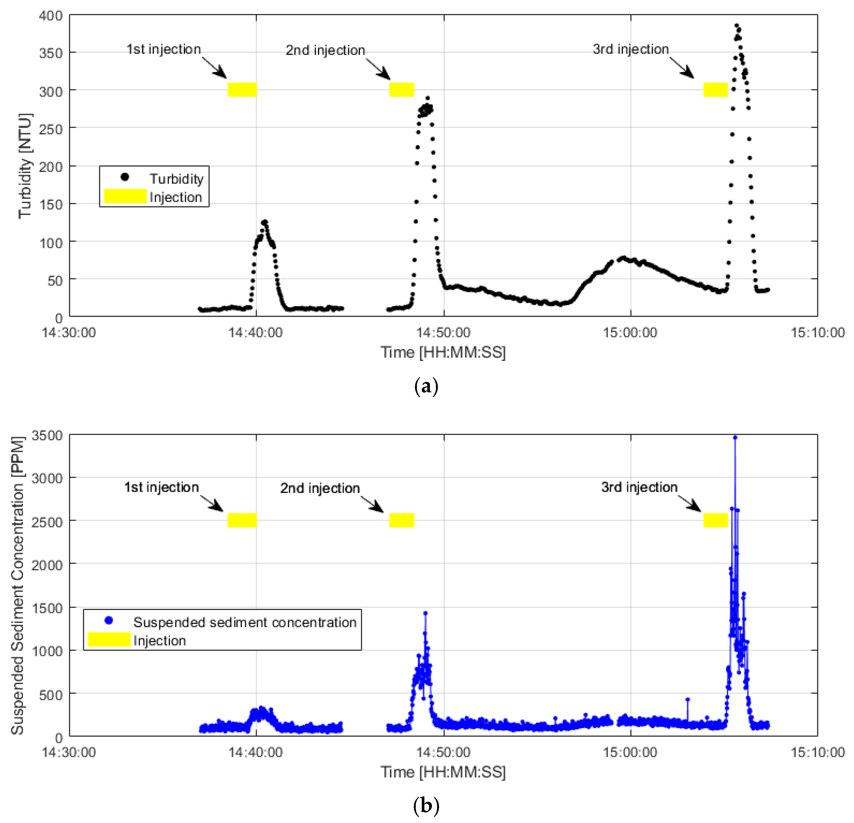

Figure 5.
Examination of flow conditions using ADCP measurement results.
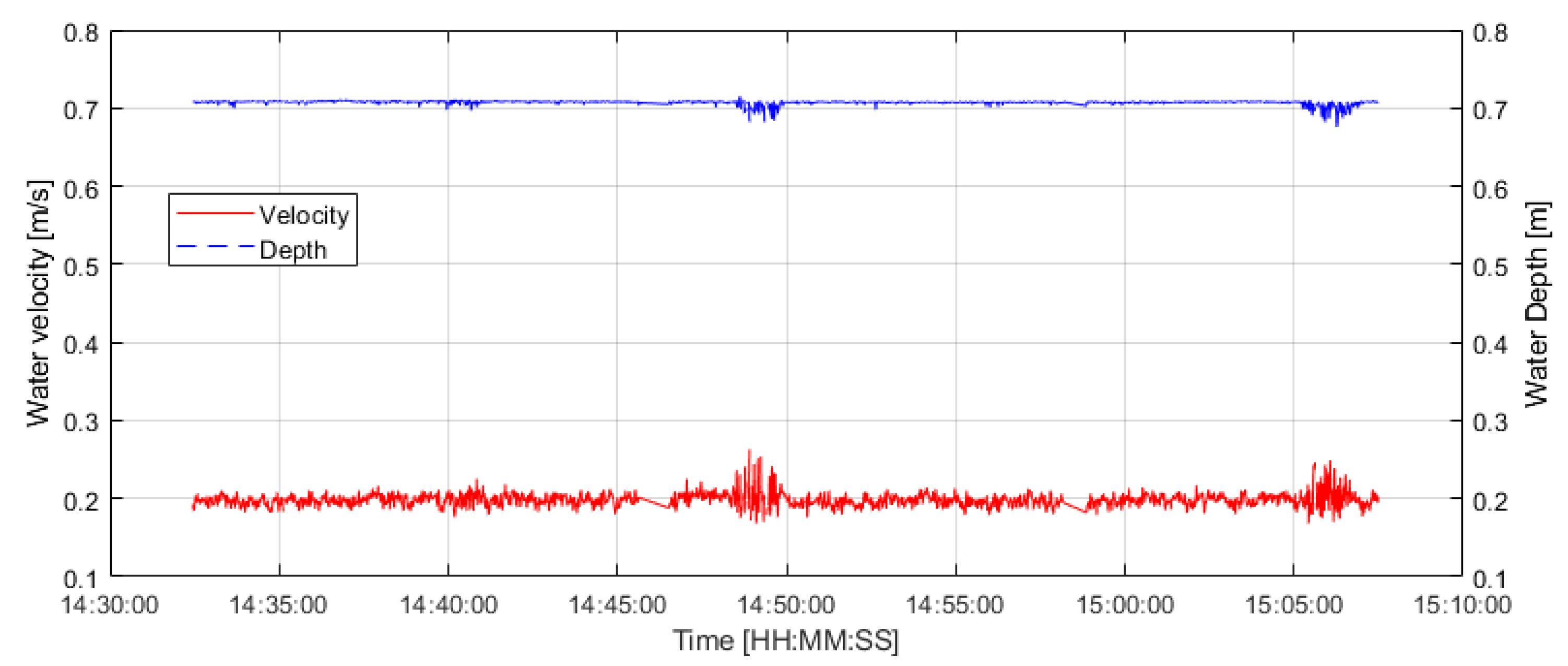
Figure 6.
Flow chart of this study.

Figure 7.
(a) Turbidity measurement results and (b) color changes in underwater images due to the changes in suspended sediment concentration and turbidity.
Figure 7.
(a) Turbidity measurement results and (b) color changes in underwater images due to the changes in suspended sediment concentration and turbidity.
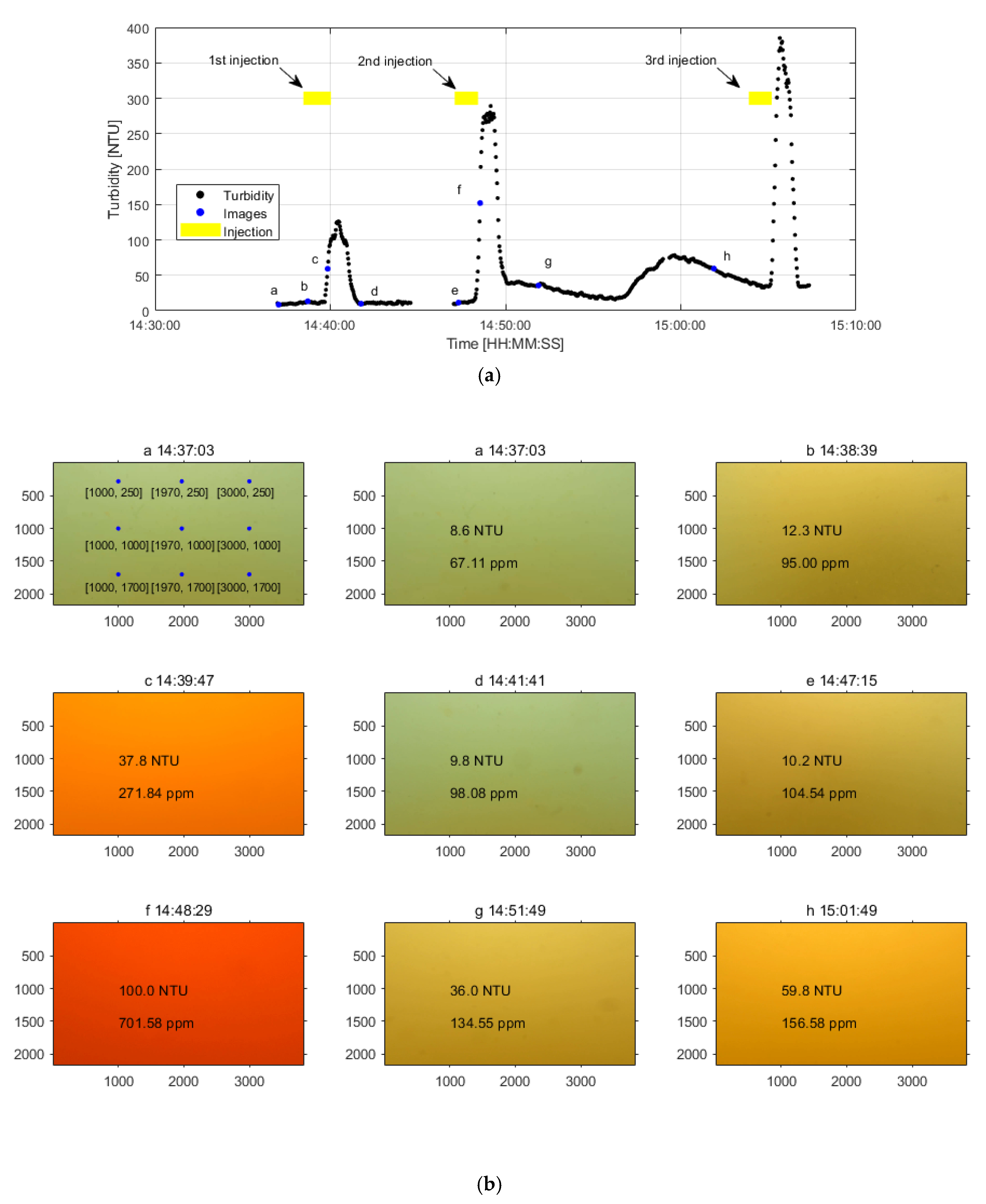
Figure 8.
Changes in RGB and gray scale values due to the turbidity change at (a) [1000, 250], (b) [1970, 250], (c) [3000, 250], (d) [1000, 1000], (e) [1970, 1000], (f) [3000, 1000], (g) [1000, 1700], (h) [1970, 1700], and (i) [3000, 1700].
Figure 8.
Changes in RGB and gray scale values due to the turbidity change at (a) [1000, 250], (b) [1970, 250], (c) [3000, 250], (d) [1000, 1000], (e) [1970, 1000], (f) [3000, 1000], (g) [1000, 1700], (h) [1970, 1700], and (i) [3000, 1700].
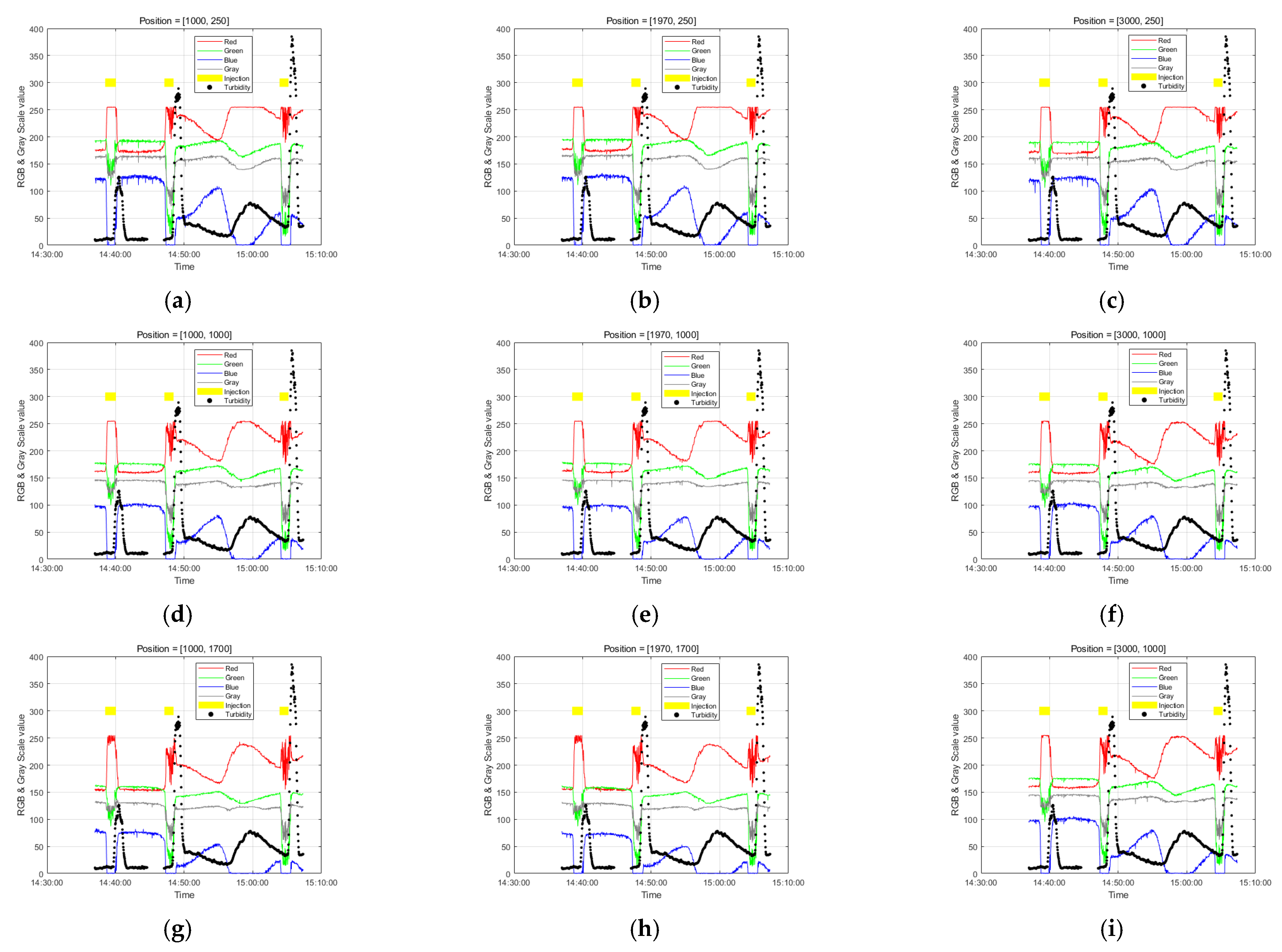
Figure 9.
Red value changes in the underwater images captured by Video 1 (at 18 m) and Video 2 (at 31.8 m).
Figure 9.
Red value changes in the underwater images captured by Video 1 (at 18 m) and Video 2 (at 31.8 m).

Figure 10.
Sections used for model development and verification, and the results reflecting the time difference between the image and turbidity measurement.
Figure 10.
Sections used for model development and verification, and the results reflecting the time difference between the image and turbidity measurement.

Figure 11.
Model verification results: (a) RGB Gray scale model, (b) RGB model, (c) RG model, (d) GB model and (e) RB model.
Figure 11.
Model verification results: (a) RGB Gray scale model, (b) RGB model, (c) RG model, (d) GB model and (e) RB model.


Figure 12.
Turbidity-concentration relationships based on average suspended sediment particle size (a) power-law, (b) second-order polynomial, and (c) first-order polynomial.
Figure 12.
Turbidity-concentration relationships based on average suspended sediment particle size (a) power-law, (b) second-order polynomial, and (c) first-order polynomial.

Figure 13.
Concentration estimated using the predicted turbidity by the developed model: (a) power-law, (b) second-order polynomial, and (c) first-order polynomial.
Figure 13.
Concentration estimated using the predicted turbidity by the developed model: (a) power-law, (b) second-order polynomial, and (c) first-order polynomial.

Figure 14.
(a) Vertical flow velocity distribution and (b) horizontal flow velocity distribution.

Figure 15.
Predicted suspended sediment concentration of (a) vertical distribution, and (b) horizontal distribution.
Figure 15.
Predicted suspended sediment concentration of (a) vertical distribution, and (b) horizontal distribution.
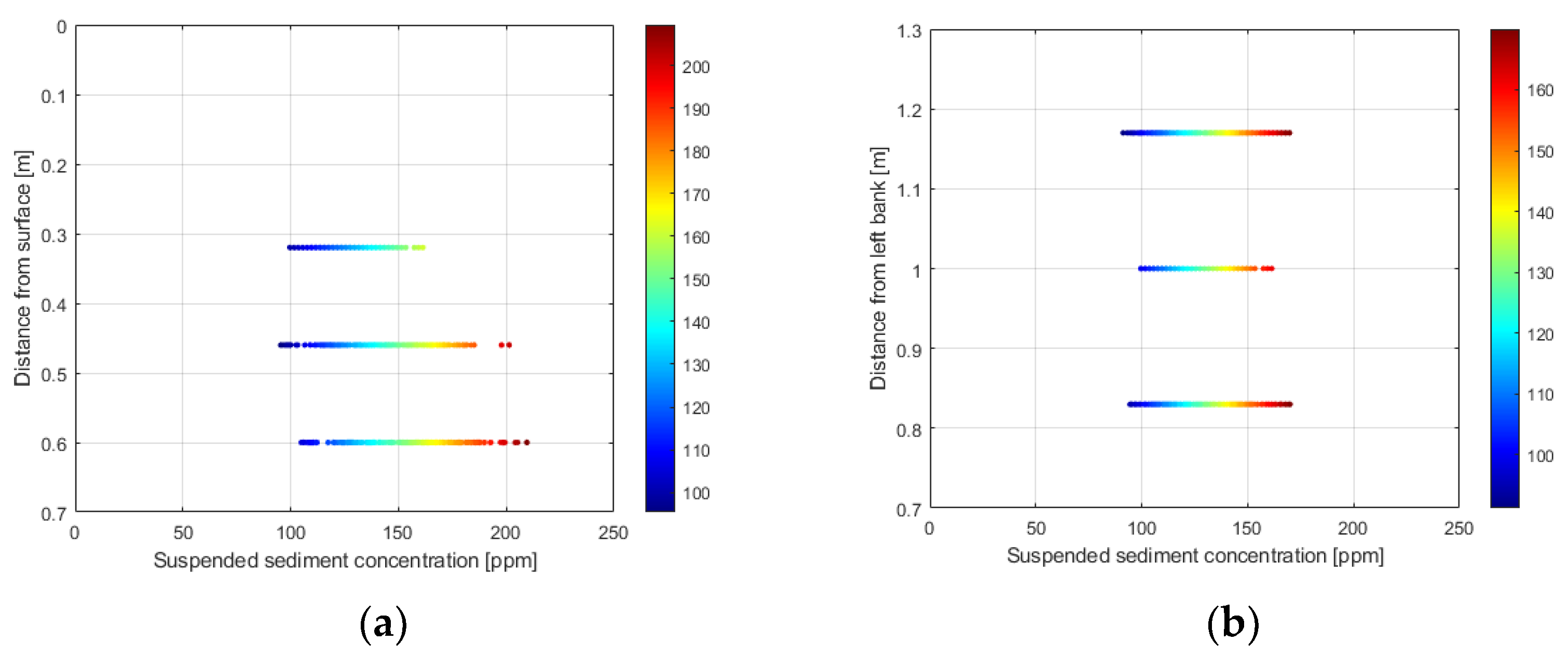
Figure 16.
R value change at the (1000, 1000) pixel during the injection of the sediment mixture.

Table 1.
Adjusted R-squared values of the developed models.
| Position (x, y) | Combination of Independent Variables | ||||
|---|---|---|---|---|---|
| (R, G, B, Gray) | (R, G, B) | (R, G) | (G, B) | (R, B) | |
| [3000, 250] | 0.9655 | 0.9655 | 0.9605 | 0.9644 | 0.9610 |
| [3000, 1000] | 0.9570 | 0.9569 | 0.9480 | 0.9399 | 0.9385 |
| [3000, 1700] | 0.9683 | 0.9680 | 0.9553 | 0.8770 | 0.9645 |
| [1000, 250] | 0.9581 | 0.9680 | 0.9541 | 0.9576 | 0.9534 |
| [1000, 1000] | 0.9529 | 0.9527 | 0.9487 | 0.9427 | 0.9227 |
| [1000, 1700] | 0.9674 | 0.9674 | 0.9522 | 0.8741 | 0.9631 |
| [1970, 250] | 0.9685 | 0.9684 | 0.9605 | 0.9664 | 0.9653 |
| [1970, 1000] | 0.9478 | 0.9460 | 0.9438 | 0.9397 | 0.9189 |
| [1970, 1700] | 0.9679 | 0.9674 | 0.9554 | 0.8777 | 0.9647 |
Table 2.
Results of multicollinearity assessment for the developed models.
| Variance Inflation Factor | |||||
|---|---|---|---|---|---|
| (RGB Gray) | (RGB) | (RG) | (GB) | (RB) | |
| R | 1606 | 53 | 3.4 | - | 17.2 |
| G | 155 | 26 | 3.4 | 8.4 | - |
| B | 3369 | 130 | - | 8.4 | 17.2 |
| GR | 1028 | - | - | - | - |
Publisher’s Note: MDPI stays neutral with regard to jurisdictional claims in published maps and institutional affiliations. |
© 2022 by the authors. Licensee MDPI, Basel, Switzerland. This article is an open access article distributed under the terms and conditions of the Creative Commons Attribution (CC BY) license (https://creativecommons.org/licenses/by/4.0/).
Share and Cite
MDPI and ACS Style
Kang, W.; Lee, K.; Kim, J. Prediction of Suspended Sediment Concentration Based on the Turbidity-Concentration Relationship Determined via Underwater Image Analysis. Appl. Sci. 2022, 12, 6125. https://doi.org/10.3390/app12126125
AMA Style
Kang W, Lee K, Kim J. Prediction of Suspended Sediment Concentration Based on the Turbidity-Concentration Relationship Determined via Underwater Image Analysis. Applied Sciences. 2022; 12(12):6125. https://doi.org/10.3390/app12126125
Chicago/Turabian StyleKang, Woochul, Kyungsu Lee, and Jongmin Kim. 2022. "Prediction of Suspended Sediment Concentration Based on the Turbidity-Concentration Relationship Determined via Underwater Image Analysis" Applied Sciences 12, no. 12: 6125. https://doi.org/10.3390/app12126125
Note that from the first issue of 2016, this journal uses article numbers instead of page numbers. See further details here.