Determination of Workspaces and Intersections of Robot Links in a Multi-Robotic System for Trajectory Planning

Abstract

One of the problems in the development of multi-robotic systems is the safe navigation of a group of robots. To solve it, the restrictions imposed by the structural elements of its agents are determined. The article presents a multi-robotic system consisting of parallel and serial robots installed on mobile platforms. The parallel robot is made based on a tripod with the ability to rotate the robot’s base relative to the horizontal axis. The analysis of its working and technological area is carried out, taking into account singularity zones. The developed algorithms for determining the workspaces are based on deterministic methods for approximating the set of solutions to systems of nonlinear inequalities. In this case, restrictions in spaces of different coordinates are presented in the form of n-dimensional boxes. Approaches to solving two problems are proposed to determine the possible intersection of links for the collaborative performance of tasks by a multi-robotic system. The first task is to determine the intersection of the links for the given positions and the relative position of the manipulators. The second is in determining the minimum distance between the technological areas of manipulators, which consist of the workspace and all possible positions of the intermediate links.

1. Introduction

Currently, an important and relevant area for solving many practical problems is multi-robotic systems. These systems have found applications in broad areas, including military surveillance, reconnaissance, rescue operations, warehousing, air traffic control, cluster telescopes, satellite formations in search and rescue operations, and the formation of autonomous unmanned aerial vehicles (UAVs). A multi-robotic multi-agent system can be described as a group of intelligent robots (agents) capable of interacting with each other and jointly to implement various tasks [1]. Interest in the problem of coordinating the movement of a large number of mobile autonomous vehicles through distributed control has raised several questions about the formation, maintenance, and modification, in real time, of vehicles of all types and has been investigated by many scientists. So, in some particular work [2], the distributed structural stabilization of the formations of a set of vehicles is considered using the structural potential functions obtained from the graphs of the formation of vehicles. In [3], an artificial potential function (APF) approach for reservoir control was considered. The formulation of the coordination problem and the presentation of feedback laws for solving problems with local information are discussed in [4]. If there is a communication channel between two group members, then both members gain access to each other’s information. This bi-directional communication leads to the creation of a special interconnection structure. Using this structure, a design method has been developed that achieves passivity and, therefore, stability of an interconnected system. There are several approaches to solving the formation control problem, such as behavior-based control [5], virtual structure-based control [6], and follower–leader control [7]. In [8], rigid and consistent education constraints are considered that can be modeled using directed graphs. One can also highlight the work on the formation of a circular structure. So, in [9], the control of the formation of a circular structure and the corresponding control law for its achievement are presented.

Safe navigation of a group of robots and the determination of the workspace of each of the robots are important tasks when building a control system for a multi-robotic system. To solve these problems, it is required to determine the constraints imposed by the structural elements of its agents. To exclude collisions between agents and external objects, it is necessary to determine the boundaries of the technological space of robots during movement, taking into account the geometric parameters and configuration of robots. Many scientists have proposed methods for constructing the workspace of robots [10,11,12]. A simple depiction of constraints was considered in [13] for a planar 3-RPR mechanism. The study of interval analysis as an effective tool for approximating the workspace is shown in [14,15,16]. Algorithms based on deterministic methods for approximating the set of solutions to systems of nonlinear inequalities can be effectively used to determine the workspace. The use of deterministic optimization algorithms based on the concept of nonuniform coverings [17] to determine the workspace of parallel robots is presented in [18,19]. Let us consider applying an approach based on the concept of nonuniform coverings to determine the working and technological areas of robots that are part of a multi-robotic system and then identify the positions at which a collision of robots is possible.

The paper is organized as follows—Section 2 presents a conceptual model of a multi-robotic system. The kinematic relationships of the parallel manipulator are presented in Section 3. The developed approach to determining the intersections of links is considered in Section 4. An algorithm is described for implementing the developed approaches to determining the workspace, taking into account the interference of links in Section 5. Section 6 shows the results of simulation of the workspace and technological space of the parallel manipulator, taking into account the rotation of the movable platform. Section 7 considers the determination of the workspace and technological space of the serial manipulator. Two problems were solved relating to the interference of manipulator links as part of a multi-robotic system in Section 8. The first problem is solved for the given positions of each of the manipulators, and the second is taking into account all the achievable positions of the manipulators using the technological spaces defined in the previous sections. A discussion on the results is provided in Section 9.

2. Formulation of the Problem

Consider a multi-robotic system with a heterogeneous structure that consists of parallel and serial robots installed on mobile platforms (Figure 1). A planar serial robot (Figure 1a) contains a horizontal base 1, which is pivotally connected at point $A^{\prime }$ with a serial manipulator 2 with rotary joints having a gripper at the end. The parallel robot (Figure 1b) is made in the form of a tripod with the ability to rotate the base relative to the horizontal axis. It contains a movable horizontal base 4, which is pivotally connected to the vertical base 5 with the possibility of its deviation from the vertical. The vertical base 5 has a drive 6. On the vertical base 5, a tripod 7 is installed. The end effector 8 is hingedly mounted on the working platform 9 of tripod 7 with the possibility of rotation about an axis perpendicular to the working platform 9 of the tripod. On the platform of the tripod, a drive 10 is installed, which ensures the rotation of the end effector 8. The grip 11 is fixed at the free end of the end effector 8.

Each of the robots must reach the required position of end-effectors in the process of performing the required operations. However, the location of the mobile platforms and the trajectory of the end-effector to achieve this position may be different. However, we should choose such an arrangement of platforms and trajectories that exclude collisions between manipulators and external objects. Further, the paper will consider the proposed approaches to the determination of robot links interference and technological workspaces of robots taking into account the intersection checking in a multi-robotic system for trajectory planning.

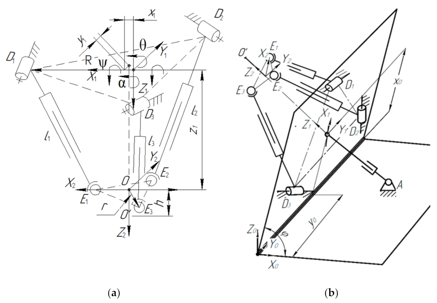
3. Parallel Manipulator Mathematical Model

Let us consider the scheme of a parallel manipulator based on a tripod (Figure 2). The tripod includes three rods of variable length $l_1, l_2, l_3$, which are connected by rotary joints $D_1, D_2, D_3$ to the base and spherical joints $E_1, E_2, E_3$ to the working platform. The base and work platform are equilateral triangles. When changing the lengths of the rods, the working platform moves along the $Z_1$ axis at a distance $z_1$, and rotates around the $X_1$ axis at an angle $\psi$ and around $Y_1$ at an angle $\theta$. In addition, there are additional degrees of freedom—displacement along the $X_1$ axes at a distance $x_1$ and along $Y_1$ at a distance $y_1$ and rotation relative to $Z_1$ by an angle $\alpha$, which are determined by the formulas [20].

$$\alpha =Ta{n}^{-1}\left(\frac{\sin \psi \sin \theta }{\cos \psi +\cos \theta }\right)$$

(1)

$$x_1=\frac{\mathrm{r}}{2}\left(\cos \theta \cos \alpha +\sin \psi \sin \theta \sin \alpha -\cos \psi \cos \alpha \right)$$

(2)

$$y_1=-r\cos \psi \sin \alpha$$

(3)

The input coordinates are the lengths of the drive links $l_1$, $l_2$, $l_3$, the output coordinates are the coordinates of the point $O^{\prime }$ of the end effector: $x_{O^{\prime }}, y_{O^{\prime }}, z_{O^{\prime }}$. Point $O^{\prime }$ is located at a distance $h$ from the center of the movable platform. To determine the workspace, it is necessary to first determine the set of permissible values of the linear and angular coordinates of the center $O$ of the movable platform, and then, for these values, determine the set of coordinates $O^{\prime }$ of the end effector. Coordinates $O^{\prime }$ in the moving coordinate system, $X_2, Y_2, Z_2,$

$${\mathit{O}}^{\prime \left(2\right)}={\left[\begin{array}{cc}\begin{array}{cc}0& 0\end{array}& \begin{array}{cc}h& 1\end{array}\end{array}\right]}^T.$$

(4)

Calculate the coordinates of point $O^{\prime }$ in the coordinate system $X_1{Y}_1{Z}_1,$

$${\mathit{O}}^{\prime \left(\mathbf{1}\right)}={\mathit{M}}_{\mathbf{2}\_\mathbf{1}}{\mathit{O}}^{\prime \left(\mathbf{2}\right)},$$

(5)

where ${\mathit{M}}_{\mathbf{2}\_\mathbf{1}}$ is the transition matrix from the moving coordinate system $X_2{Y}_2{Z}_2$ to the fixed system $X_1{Y}_1{Z}_1$ which includes matrices of displacements and rotations along the $X_1, Y_1, Z_1,$

$${\mathit{M}}_{\mathbf{2}\_\mathbf{1}}=\left[\begin{array}{cc}\begin{array}{cc}\cos \theta \cos \alpha +\sin \psi \sin \theta \sin \alpha & -\cos \theta \sin \alpha +\sin \psi \sin \theta \cos \alpha \\ \cos \psi \sin \alpha & \cos \psi \cos \alpha \end{array}& \begin{array}{cc}\sin \theta \cos \psi & x_1\\ -\sin \psi & y_1\end{array}\\ \begin{array}{cc}-\sin \theta \cos \alpha +\sin \psi \cos \theta \sin \alpha & \sin \theta \sin \alpha +\sin \psi \cos \theta \cos \alpha \\ 0& 0\end{array}& \begin{array}{cc}\cos \theta \cos \psi & z_1\\ 0& 1\end{array}\end{array}\right]$$

(6)

After transformation taking into account (4)–(6), we get,

$${\mathit{O}}^{\prime \left(\mathbf{1}\right)}=\left[\begin{array}{c}{x}_1+\sin \theta \cos \psi h\\ y_1-\sin \psi h\\ \begin{array}{c}{z}_1+\cos \theta \cos \psi h\\ 1\end{array}\end{array}\right]$$

(7)

Let us introduce restrictions on the geometric parameters of the mechanism,

$$\left\{\begin{array}{c}{l}_i-l_{\max }\le 0\\ l_{\min }-l_i\le 0\end{array}\right.$$

(8)

where $l_{\min }, l_{\max }$ are determined by the design parameters of the mechanism; $l_i$ is the length of the i-th rod, which is defined as,

$$l_i=\sqrt{{\left(x_{Ei}-x_{Di}\right)}^2+{\left(y_{Ei}-y_{Di}\right)}^2+{\left(z_{Ei}-z_{Di}\right)}^2},$$

(9)

where $x_{Ei}, y_{Ei}, z_{Ei}$—coordinates of the centers of the joints, point $E_i$; $x_{Di}, y_{Di}, z_{Di}$—coordinates of the centers of the joints, point $D_i$ in a fixed coordinate system.

We define the coordinates of the joints $E_i$ in the moving coordinate system $X_2^{\prime }{Y}_2^{\prime }{Z}_2^{\prime }$ ${\mathit{E}}_{\mathbf{1}}^{\left(\mathbf{2}\right)}={\left[\begin{array}{cc}r& \begin{array}{cc}0& \begin{array}{cc}0& 1\end{array}\end{array}\end{array}\right]}^T$, ${\mathit{E}}_{\mathbf{2}}^{\left(\mathbf{2}\right)}={\left[\begin{array}{cc}-0.5r& \begin{array}{cc}0.5\sqrt{3}r& \begin{array}{cc}0& 1\end{array}\end{array}\end{array}\right]}^T$, ${\mathit{E}}_{\mathbf{3}}^{\left(2\right)}={\left[\begin{array}{cc}-0.5r& \begin{array}{cc}-0.5\sqrt{3}r& \begin{array}{cc}0& 1\end{array}\end{array}\end{array}\right]}^T$.

We denote in (6) $M_{11}=\cos \theta \cos \alpha +\sin \psi \sin \theta \sin \alpha$; $M_{12}=-\cos \theta \sin \alpha +\sin \psi \sin \theta \cos \alpha$; $M_{13}=\sin \theta \cos \psi$; $M_{21}=\cos \psi \sin \alpha$; $M_{22}=\cos \psi \cos \alpha$; $M_{23}=-\sin \psi$; $M_{31}=-\sin \theta \cos \alpha +\sin \psi \cos \theta \sin \phi$; $M_{32}=\sin \theta \sin \alpha +\sin \psi \cos \theta \cos \alpha$; $M_{33}=\cos \theta \cos \psi$.

Let us express the coordinates of the joints $E_i$ in the moving coordinate system $X_1{Y}_1{Z}_1$

$${\mathit{E}}_{\mathbf{1}}^{\left(\mathbf{1}\right)}={\mathit{M}}_{\mathbf{2}\_\mathbf{1}}{\mathit{E}}_{\mathbf{1}}^{\left(\mathbf{2}\right)}={\left[\begin{array}{cc}{x}_1+M_{11}r& \begin{array}{cc}{y}_1+M_{21}r& \begin{array}{cc}{z}_1+M_{31}r& 1\end{array}\end{array}\end{array}\right]}^{T }={\left[\begin{array}{cc}{x}_1+M_{11}r& \begin{array}{cc}0& \begin{array}{cc}{z}_1+M_{31}r& 1\end{array}\end{array}\end{array}\right]}^T,$$

(10)

$${\mathit{E}}_{\mathbf{2}}^{\left(\mathbf{1}\right)}={\mathit{M}}_{\mathbf{2}\_\mathbf{1}}{\mathit{E}}_{\mathbf{2}}^{\left(\mathbf{2}\right)}={\left[\begin{array}{cc}{x}_1-0.5r\left(M_{11}-\sqrt{3}{M}_{12}\right)& \begin{array}{cc}{y}_1-0.5r\left(M_{21}-\sqrt{3}{M}_{22}\right)& \begin{array}{cc}{z}_1-0.5r\left(M_{31}-\sqrt{3}{M}_{32}\right)& 1\end{array}\end{array}\end{array}\right]}^T,$$

(11)

$${\mathit{E}}_{\mathbf{3}}^{\left(\mathbf{1}\right)}={\mathit{M}}_{\mathbf{2}\_\mathbf{1}}{\mathit{E}}_{\mathbf{3}}^{\left(\mathbf{2}\right)}={\left[\begin{array}{cc}{x}_1-0.5r\left(M_{11}+\sqrt{3}{M}_{12}\right)& \begin{array}{cc}{y}_1-0.5r\left(M_{21}+\sqrt{3}{M}_{22}\right)& \begin{array}{cc}{z}_1-0.5r\left(M_{31}+\sqrt{3}{M}_{32}\right)& 1\end{array}\end{array}\end{array}\right]}^{T }$$

(12)

Determine the coordinates of the joints D_i in the moving coordinate system $X_1{Y}_1{Z}_1$:

$${\mathit{D}}_{\mathbf{1}}^{\left(\mathbf{1}\right)}={\left[\begin{array}{cc}R& \begin{array}{cc}0& \begin{array}{cc}0& 1\end{array}\end{array}\end{array}\right]}^T,{\mathit{D}}_{\mathbf{2}}^{\left(\mathbf{1}\right)}={\left[\begin{array}{cc}-0.5R& \begin{array}{cc}0.5\sqrt{3}R& \begin{array}{cc}0& 1\end{array}\end{array}\end{array}\right]}^T,{\mathit{D}}_{\mathbf{3}}^{\left(\mathbf{1}\right)}={\left[\begin{array}{cc}-0.5R& \begin{array}{cc}-0.5\sqrt{3}R& \begin{array}{cc}0& 1\end{array}\end{array}\end{array}\right]}^T.$$

(13)

Substituting (10)–(13) into (9), we obtain,

$$l_1=\sqrt{{\left(x_1+M_{11}r-R\right)}^2+{\left(z_1+M_{31}r\right)}^2},$$

(14)

$$l_2={\left({\left(x_1-0.5r\left(M_{11}-\sqrt{3}{M}_{12}\right)+0.5R\right)}^2+{\left(y_1-0.5r\left(M_{21}-\sqrt{3}{M}_{22}\right)-\frac{\sqrt{3}}{2}R\right)}^2+{\left(z_1-0.5r\left(M_{31}-\sqrt{3}{M}_{32}\right)\right)}^2\right)}^{\raisebox{1ex}{$1$}\!\left/ \!\raisebox{-1ex}{$2$}\right.}$$

(15)

$$l_3={\left({\left(x_1-0.5r\left(M_{11}+\sqrt{3}{M}_{12}\right)+0.5R\right)}^2+{\left(y_1-0.5r\left(M_{21}+\sqrt{3}{M}_{22}\right)-\frac{\sqrt{3}}{2}R\right)}^2+{\left(z_1-0.5r\left(M_{31}+\sqrt{3}{M}_{32}\right)\right)}^2\right)}^{\raisebox{1ex}{$1$}\!\left/ \!\raisebox{-1ex}{$2$}\right.}$$

(16)

Similarly, we calculate the coordinates of the point $O^{\prime }$ in the fixed coordinate system $X_0{Y}_0{Z}_0$:

$${\mathit{O}}_{\mathbf{0}}^{\prime }={\mathit{M}}_{\mathbf{1}\_\mathbf{0}}{\mathit{O}}_{\mathbf{1}}^{\prime },$$

(17)

where ${\mathit{M}}_{\mathbf{1}\_\mathbf{0}}$ is the transition matrix from the moving coordinate system $X_1{Y}_1{Z}_1$ to the fixed system $X_0{Y}_0{Z}_0$, which includes matrices of displacement along the $X_0$ and $Y_0$ axes and rotation around the $Y_0$ axis,

$${\mathit{M}}_{\mathbf{1}\_\mathbf{0}}=\left[\begin{array}{cc}\begin{array}{cc}\cos \phi & 0\\ 0& 1\end{array}& \begin{array}{cc}-\sin \phi & x_0\cos \phi \\ 0& y_0\end{array}\\ \begin{array}{cc}\sin \phi & 0\\ 0& 0\end{array}& \begin{array}{cc}\cos \phi & \sin \phi x_0\\ 0& 1\end{array}\end{array}\right]$$

(18)

After transformation, taking into account (7), (17) and (18), we obtain,

$${\mathit{O}}_{\mathbf{0}}^{\prime }=\left[\begin{array}{c}\cos \phi \left(x_1+x_0+\sin \theta \cos \psi h\right)-\sin \phi \left(z_1+\cos \theta \cos \psi h\right)\\ y_1-\sin \psi h+y_0\\ \begin{array}{c}\cos \phi \left(z_1+\cos \theta \cos \psi h\right)+\sin \phi \left(x_1+x_0+\sin \theta \cos \psi h\right)\\ 1\end{array}\end{array}\right]$$

(19)

The coordinates of the joints $D_i$ and $E_i$ in the fixed coordinate system $X_0{Y}_0{Z}_0$ are defined as:

$${\mathit{D}}_{\mathbf{1}}^{\left(\mathbf{0}\right)}={\mathit{M}}_{\mathbf{1}\_\mathbf{0}}{\mathit{D}}_{\mathbf{1}}^{\left(\mathbf{1}\right)}={\left[\begin{array}{cc}\cos \phi \left(R+x_0\right)& \begin{array}{cc}0& \begin{array}{cc}\sin \phi \left(R+x_0\right)& 1\end{array}\end{array}\end{array}\right]}^T,$$

(20)

$${\mathit{D}}_{\mathbf{2}}^{\left(\mathbf{0}\right)}={\mathit{M}}_{\mathbf{1}\_\mathbf{0}}{\mathit{D}}_{\mathbf{2}}^{\left(\mathbf{1}\right)}={\left[\begin{array}{cc}\cos \phi \left(x_0-0.5R\right)& \begin{array}{cc}0.5\sqrt{3}R& \begin{array}{cc}\sin \phi \left(x_0-0.5R\right)& 1\end{array}\end{array}\end{array}\right]}^T$$

(21)

$${\mathit{D}}_{\mathbf{3}}^{\left(\mathbf{0}\right)}={\mathit{M}}_{\mathbf{1}\_\mathbf{0}}{\mathit{D}}_{\mathbf{3}}^{\left(\mathbf{1}\right)}={\left[\begin{array}{cc}\cos \phi \left(x_0-0.5R\right)& \begin{array}{cc}-0.5\sqrt{3}R& \begin{array}{cc}\sin \phi \left(x_0-0.5R\right)& 1\end{array}\end{array}\end{array}\right]}^T$$

(22)

$${\mathit{E}}_{\mathbf{1}}^{\left(\mathbf{0}\right)}={\mathit{M}}_{\mathbf{1}\_\mathbf{0}}{\mathit{E}}_{\mathbf{1}}^{\left(\mathbf{1}\right)}=\left[\begin{array}{c}\cos \phi \left(x_1+M_{11}r+x_0\right)-\sin \phi \left(z_1+M_{31}r\right)\\ 0\\ \begin{array}{c}\sin \phi \left(x_1+M_{11}r+x_0\right)+\cos \phi \left(z_1+M_{31}r\right)\\ 1\end{array}\end{array}\right],$$

(23)

$${\mathit{E}}_{\mathbf{2}}^{\left(\mathbf{0}\right)}={\mathit{M}}_{\mathbf{1}\_\mathbf{0}}{\mathit{E}}_{\mathbf{2}}^{\left(\mathbf{1}\right)}=\left[\begin{array}{c}\cos \phi \left(x_1-0.5r\left(M_{11}-\sqrt{3}{M}_{12}\right)+x_0\right)-\sin \phi \left(z_1-0.5r\left(M_{31}-\sqrt{3}{M}_{32}\right)\right)\\ y_1-0.5r\left(M_{21}-\sqrt{3}{M}_{22}\right)\\ \begin{array}{c}\sin \phi \left(x_1-0.5r\left(M_{11}-\sqrt{3}{M}_{12}\right)+x_0\right)+\cos \phi \left(z_1-0.5r\left(M_{31}-\sqrt{3}{M}_{32}\right)\right)\\ 1\end{array}\end{array}\right],$$

(24)

$${\mathit{E}}_{\mathbf{3}}^{\left(\mathbf{0}\right)}={\mathit{M}}_{\mathbf{1}\_\mathbf{0}}{\mathit{E}}_{\mathbf{3}}^{\left(\mathbf{1}\right)}=\left[\begin{array}{c}\cos \phi \left(x_1-0.5r\left(M_{11}+\sqrt{3}{M}_{12}\right)+x_0\right)-\sin \phi \left(z_1-0.5r\left(M_{31}+\sqrt{3}{M}_{32}\right)\right)\\ y_1-0.5r\left(M_{21}+\sqrt{3}{M}_{22}\right)\\ \begin{array}{c}\sin \phi \left(x_1-0.5r\left(M_{11}+\sqrt{3}{M}_{12}\right)+x_0\right)+\cos \phi \left(z_1-0.5r\left(M_{31}+\sqrt{3}{M}_{32}\right)\right)\\ 1\end{array}\end{array}\right].$$

(25)

We calculate the integers corresponding to the coordinates of the point $O^{\prime }$ to describe the form of a partially ordered set of integers,

$$\left\{\begin{array}{c}{x}_{O^{\prime }}^{\left(Z\right)}=\left[\frac{x_{O^{\prime }}}{\delta }\right],x_{O^{\prime }}\in ℝ, x_{O^{\prime }}^{\left(Z\right)}\in \mathbb{Z} \\ y_{O^{\prime }}^{\left(Z\right)}=\left[\frac{y_{O^{\prime }}}{\delta }\right],y_{O^{\prime }}\in ℝ, y_{O^{\prime }}^{\left(Z\right)}\in \mathbb{Z} \\ z_{O^{\prime }}^{\left(Z\right)}=\left[\frac{z_{O^{\prime }}}{\delta }\right],z_{O^{\prime }}\in ℝ, z_{O^{\prime }}^{\left(Z\right)}\in \mathbb{Z} \end{array}\right.,$$

(26)

where $\delta$ is the approximation accuracy.

In addition to restrictions on the permissible ranges of drive lengths, it is necessary to exclude the mechanism from falling into singularity zones in which the control of the mechanism is lost. We use the method proposed by C. Gosselin [21], which is based on the analysis of the Jacobi matrix of the mechanism obtained by differentiating the constraint equations and describing the transition from generalized velocities in driving kinematic pairs to angular or linear velocities of the end effector. According to Gosselin’s classification [21], the tripod is characterized by singularities of only the second type, for which the Jacobi matrix is equal to zero.

The determinant of the Jacobi matrix has the form,

$$\det \left(J_A\right)=\left[\begin{array}{ccc}\frac{\partial F_1}{\partial z}& \frac{\partial F_1}{\partial \psi }& \frac{\partial F_1}{\partial \theta }\\ \frac{\partial F_2}{\partial z}& \frac{\partial F_2}{\partial \psi }& \frac{\partial F_2}{\partial \theta }\\ \frac{\partial F_3}{\partial z}& \frac{\partial F_3}{\partial \psi }& \frac{\partial F_3}{\partial \theta }\end{array}\right],$$

(27)

where $F_i$ corresponds to the bar length Formulas (14)–(16).

Because of the cumbersomeness of the formulas for each of the elements of the determinant, we present only one of them,

$$\begin{array}{c}\frac{\partial F_1}{\partial z}=z-r\left(\frac{Sb\left(Ca+Cb\right)-CbSbS{a}^2}{\left(Ca+Cb\right)\sqrt{\left(\frac{S{a}^{2}S{b}^2}{{\left(Ca+Cb\right)}^2}+1\right)}}\right)\left(\right(r\left(\frac{Cb\left(Ca+Cb\right)+S{a}^{2}S{b}^2}{\left(Ca+Cb\right)\sqrt{\left(\frac{S{a}^{2}S{b}^2}{{\left(Ca+Cb\right)}^2}+1\right)}}\right)\\ -R+\frac{r\left(Cb-Ca\cos \left(2{\tan }^{-1}\left(\frac{SaSb}{\left(Ca+Cb\right)}\right)\right)\right)}{2}{)}^2\\ +{\left(z-r\left(\frac{Sb\left(Ca+Cb\right)-CbSbS{a}^2}{\left(Ca+Cb\right)\sqrt{\left(\frac{S{a}^{2}S{b}^2}{{\left(Ca+Cb\right)}^2}+1\right)}}\right)\right)}^2{)}^{-2}\end{array}$$

where Ca = cos($\theta$); $Ca=\cos \left(\theta \right), Cb=\cos \left(\psi \right), Sa=\sin \left(\theta \right), Sb=\sin \left(\psi \right).$ Let us write down the condition for the occurrence of singularity zones,

$$\det \left(J_A\right)=0$$

(28)

Getting into a singularity zone in which condition (28) is satisfied occurs when the sign of the determinant of the Jacobi matrix is changed, therefore, it is necessary to add the condition of its constancy of sign.

The given constraints make it possible to determine constraints in the space of coordinates $z_1,\theta ,\psi$, under which we calculate the set of positions of the end effector according to (7), (19), (25). It should be noted that these restrictions do not allow us to exclude the intersection of the links of the mechanism.

4. Determination of Link Intersections

The intersections of the links of the mechanism can be divided into two groups:

-

Intersections at small angles between links connected by rotary joints; and

-

The intersection of links that are not connected.

The first group can be defined, taking into account the restrictions on the angles of rotation in the joints $E_i$:

$${\beta }_i^{\left(j\right)}\in \left[{\beta }_{min};{\beta }_{max}\right], i\in 1,2,3, j\in 1,2,3,$$

(29)

where $i$ is the index of the joint $E$, $j$ is the index for one of the three corners of the joint $E_i$.

Define the angles ${\beta }_1^{\left(j\right)}$

$${\beta }_1^{\left(1\right)}={\cos }^{-1}\left(\frac{\left(x_{D1}-x_{E1}\right)\left(x_{E2}-x_{E1}\right)+\left(y_{D1}-y_{E1}\right)\left(y_{E2}-y_{E1}\right)+\left(z_{D1}-z_{E1}\right)\left(z_{E2}-z_{E1}\right)}{\sqrt{3}R{l}_1}\right),{\beta }_1^{\left(1\right)}\in \left[0;\pi \right]$$

(30)

$${\beta }_1^{\left(2\right)}={\cos }^{-1}\left(\frac{\left(x_{D1}-x_{E1}\right)\left(x_1-x_{E1}\right)+\left(y_{D1}-y_{E1}\right)\left(y_1-y_{E1}\right)+\left(z_{D1}-z_{E1}\right)\left(z_1-z_{E1}\right)}{R{l}_1}\right), {\beta }_1^{\left(2\right)}\in \left[0;\pi \right]$$

(31)

$${\beta }_1^{\left(3\right)}={\cos }^{-1}\left(\frac{\left(x_{D1}-x_{E1}\right)\left(x_{E3}-x_{E1}\right)+\left(y_{D1}-y_{E1}\right)\left(y_{E3}-y_{E1}\right)+\left(z_{D1}-z_{E1}\right)\left(z_{E3}-z_{E1}\right)}{\sqrt{3}R{l}_1}\right),{\beta }_1^{\left(3\right)}\in \left[0;\pi \right]$$

(32)

We define the second group of intersections using an approach based on determining the minimum distance between the segments drawn between the centers of the joints of each of the links. In [22], a similar condition is used, but the approach has drawbacks. In particular, the authors propose determining the intersections of the segments on the auxiliary plane, not the distance between the nearest points. This does not allow for identifying such an intersection of links in which there is no intersection of the axes.

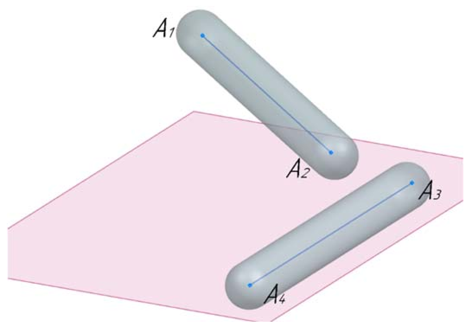
The approach proposed in the current work is as follows. Let us imagine the links in the form of a spherocylinder. Let $A_1{A}_2$ и $A_3{A}_4$ be the segments connecting the centers of the joints of the links (Figure 3).

In this case, we write the first condition for the absence of intersections as:

$$D_{link}<\sqrt{{\left(x^{\prime }\right)}^2+{\left(y^{\prime }\right)}^2+{\left(z^{\prime }\right)}^2},$$

(33)

where $D_{link}$ is the diameter of the links, $x^{\prime }$,$y^{\prime }$,$z^{\prime }$ is the distance between the nearest points of the segments along each of the axes and are defined as:

$$x^{\prime }=\left\{\begin{array}{c}\underset{i\in 1,2}{min}{x}_{Ai}-\underset{j\in 3,4}{max}{x}_{Aj} if \underset{i\in 1,2}{min}{x}_{Ai}>\underset{i\in 1,2}{max}{x}_{Ai},\\ \underset{i\in 3,4}{min}{x}_{Aj}-\underset{i\in 1,2}{max}{x}_{Ai} if \underset{i\in 3,4}{min}{x}_{Aj}>\underset{i\in 1,2}{max}{x}_{Ai},\\ 0 if \left[\underset{i\in 1,2}{min}{x}_{Ai};\underset{i\in 1,2}{max}{x}_{Ai}\right]\cap \left[\underset{i\in 3,4}{min}{x}_{Aj};\underset{j\in 3,4}{max}{x}_{Aj}\right].\end{array}\right.$$

(34)

The values $y^{\prime }$ and $z^{\prime }$ are defined similarly.

There is no intersection of the links when the minimum distance u between the segments $A_1{A}_2$ and $A_3{A}_4$ is greater than the diameter of the links $D_{link}$:

$$D_{link}>u$$

(35)

Consider two cases of relative position of links.

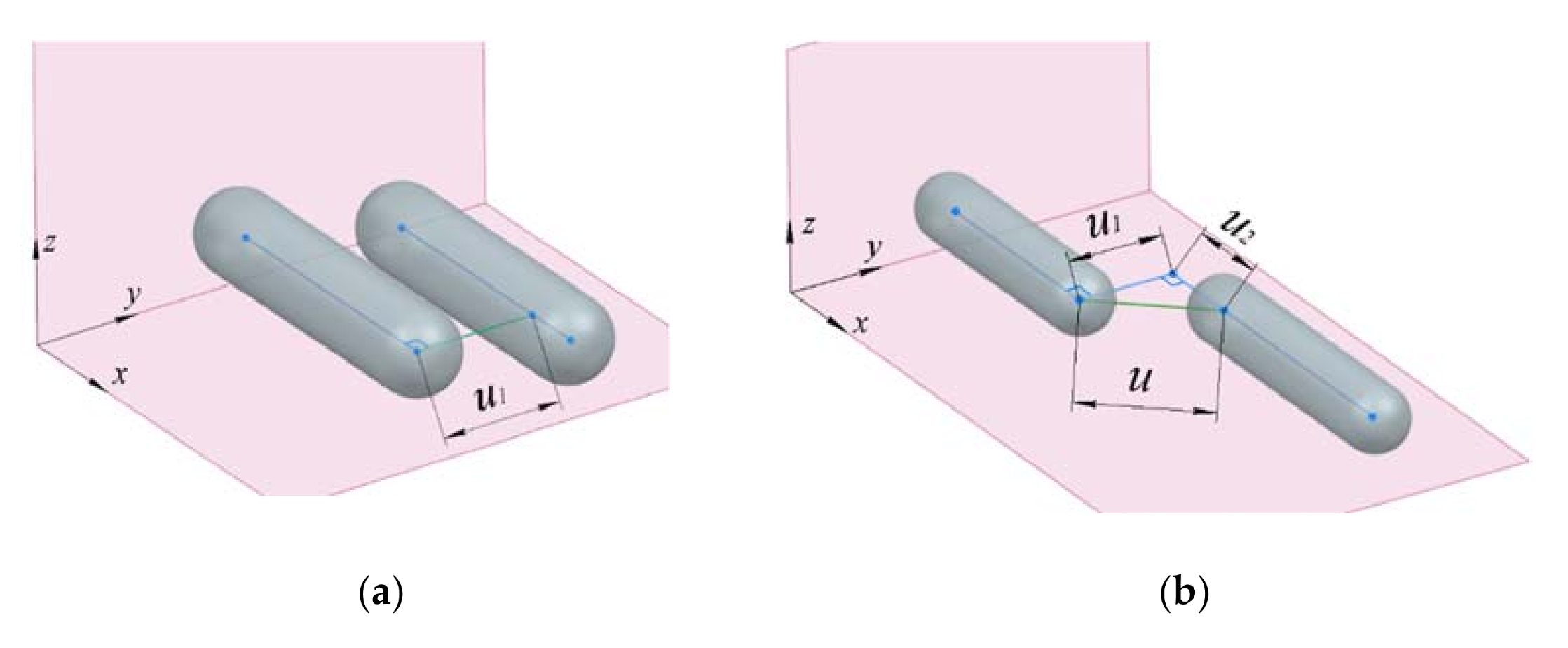
Case 1. The links are parallel in the case when the condition is fulfilled:

$$\frac{x_{A2}-x_{A1}}{x_{A4}-x_{A3}}=\frac{y_{A2}-y_{A1}}{y_{A4}-y_{A3}}=\frac{z_{A2}-z_{A1}}{z_{A4}-z_{A3}}$$

(36)

Determine the minimum distance between the segments by rotating the segments relative to the point $A_1$ so that they become perpendicular to the YOZ plane. Let us denote for points $A_2, A_3$ and $A_4$ the obtained coordinates of points after rotation as $A_{12}, A_{13}$ and $A_{14}$, respectively. Taking into account the rotation of the segments to the perpendicular position to the YOZ plane, the coordinates of the points $A_{12}, A_{13}$ and $A_{14}$ are calculated as:

$$x_{A1i}=x_{A1}+c_i^{\left(a\right)}\left(x_{Ai}-x_{A1}\right)+s_i^{\left(a\right)}\left(s_i^{\left(b\right)}\left(y_{Ai}-y_{A1}\right)+c_i^{\left(b\right)}\left(z_{Ai}-z_{A1}\right)\right),$$

(37)

$$y_{A1i}=y_{A1}+c_i^{\left(b\right)}\left(y_{Ai}-y_{A1}\right)-s_i^{\left(b\right)}\left(z_{Ai}-z_{A1}\right),$$

(38)

$$z_{A1i}=z_{A1}-s_i^{\left(a\right)}\left(x_{Ai}-x_{A1}\right)+c_i^{\left(a\right)}\left(s_i^{\left(b\right)}\left(y_{Ai}-y_{A1}\right)+c_i^{\left(b\right)}\left(z_{Ai}-z_{A1}\right)\right),$$

(39)

where $s_i^{\left(a\right)}=\sin \left({\tan }^{-1}\left(\frac{s_b\left(y_{Ai}-y_{A1}\right)+c_b\left(z_{Ai}-z_{A1}\right)}{x_{Ai}-x_{A1}}\right)\right)$, $c_i^{\left(a\right)}=\cos \left({\tan }^{-1}\left(\frac{s_b\left(y_{Ai}-y_{A1}\right)+c_b\left(z_{Ai}-z_{A1}\right)}{x_{Ai}-x_{A1}}\right)\right)$, $s_i^{\left(b\right)}=\sin \left({\tan }^{-1}\frac{y_{Ai}-y_{A1}}{z_{Ai}-z_{A1}}\right)$, $c_i^{\left(b\right)}=\cos \left({\tan }^{-1}\frac{y_{Ai}-y_{A1}}{z_{Ai}-z_{A1}}\right)$,$i\in 2, 3, 4.$ In this case, $y_{A12}=y_{A1},z_{A12}=z_{A1}$, $y_{A13}=y_{A14}$, $z_{A13}=z_{A14}$.

The distance between the segments is determined as:

$$u=\sqrt{u_1^2+u_2^2},$$

(40)

where $u_1$ is the distance between the segments $A_1{A}_{12}$ and $A_{13}{A}_{14}$ in the projection onto the YOZ plane, $u_2$ is the distance between the nearest points of the segments along the X axis. They are defined as:

$$u_1=\sqrt{{\left(y_{A13}-y_{A1}\right)}^2+{\left(z_{A13}-z_{A1}\right)}^2}$$

(41)

$$u_2=\left\{\begin{array}{c}\underset{i\in 1,12}{\min }{x}_{Ai}-\underset{j\in 13,14}{\max }{x}_{Aj} \mathrm{if} \underset{i\in 1,12}{\min }{x}_{Ai}>\underset{i\in 1,12}{\max }{x}_{Ai},\\ \underset{i\in 13,14}{\min }{x}_{Aj}-\underset{i\in 1,12}{\max }{x}_{Ai} \mathrm{if} \underset{i\in 13,14}{\min }{x}_{Aj}>\underset{i\in 1,12}{\max }{x}_{Ai},\\ 0 \mathrm{if} \left[\underset{i\in 1,12}{\min }{x}_{Ai};\underset{i\in 1,12}{\max }{x}_{Ai}\right]\cap \left[\underset{i\in 13,14}{\min }{x}_{Aj};\underset{j\in 13,14}{\max }{x}_{Aj}\right].\end{array}\right.$$

(42)

Figure 4 shows examples of verification for the first case of intersection of links. Figure 4a shows an example when $u_1>D_{link}$, and $u_2=0$, since the coordinate intervals of the segments along the $X$ axis intersect. In this case, $u=u_1$, respectively, $u>D_{link}$ and there is no intersection. Figure 4b shows an example where $u_1>0$ and $u_2>0$, while $u>D_{link}$, so there is no intersection.

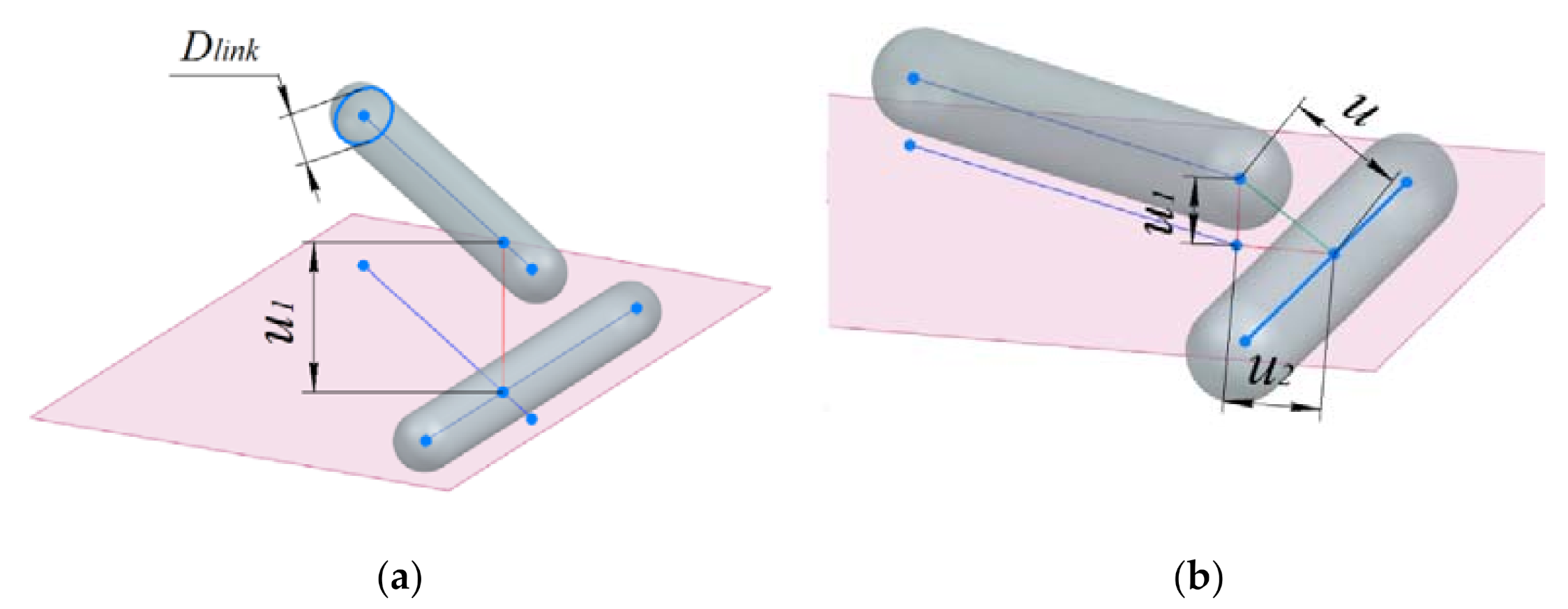
Case 2. Condition (36) is not satisfied, that is, the links are not parallel. Let us construct an auxiliary plane in which the segment $A_3{A}_4$ will lie and to which the segment $A_1{A}_2$ will be parallel. In this case, the distance between the segments can be similarly written as:

$$u=\sqrt{u_1^2+u_2^2},$$

(43)

where $u_1$ is the distance between the segment $A_1{A}_2$ and the auxiliary plane, $u_2$ is the distance between the nearest points of the segments $A_3{A}_4$ and the projection of the segment $A_1{A}_2$ onto the auxiliary plane.

To determine $u_1$, we calculate the normal vector:

$$\mathit{N}=\left[\begin{array}{c}{N}_x\\ N_y\\ N_z\end{array}\right]=\left[\begin{array}{c}\left(y_{A4}-y_{A3}\right)\left(z_{A2}-z_{A1}\right)-\left(z_{A4}-z_{A3}\right)\left(y_{A2}-y_{A1}\right)\\ \left(z_{A4}-z_{A3}\right)\left(x_{A2}-x_{A1}\right)-\left(x_{A4}-x_{A3}\right)\left(z_{A2}-z_{A1}\right)\\ \left(x_{A4}-x_{A3}\right)\left(y_{A2}-y_{A1}\right)-\left(y_{A4}-y_{A3}\right)\left(x_{A2}-x_{A1}\right)\end{array}\right]$$

(44)

Determine the distance $u_1$ using the coefficient $k$ for the length of the normal vector.

$$u_1=\sqrt{{\left(N_{x}k\right)}^2+{\left(N_{y}k\right)}^2+{\left(N_{z}k\right)}^2},$$

(45)

where $k=\frac{N_x\left(x_{A1}-x_{A3}\right)+N_y\left(y_{A1}-y_{A3}\right)+N_z\left(z_{A1}-z_{A3}\right)}{x_{A1}{N}_x+y_{A1}{N}_y+z_{A1}{N}_z}.$

Let us determine, using the coefficient $k$, the coordinates of the point $A_{11}$ as a result of the projection of the point $A_1$ onto the auxiliary plane:

$$x_{A11}=x_{A1}-N_{x}k,y_{A11}=y_{A1}-N_{y}k,z_{A11}=z_{A1}-N_{z}k.$$

(46)

To define $u_2$, rotate the construction plane around point $A_{11}$ so that it is parallel to the YOZ plane. After rotating the coordinates of the second point of the segment $A_{12}$ and points $A_{13}$ and $A_{14}$ of the second segment, we define as:

$$x_{A12}=x_{A11}+c^{\left(a\right)}\left(x_{Ai}-x_{A1}\right)+s^{\left(a\right)}\left(s^{\left(b\right)}\left(y_{Ai}-y_{A1}\right)+c^{\left(b\right)}\left(z_{Ai}-z_{A1}\right)\right),$$

(47)

$$y_{A12}=y_{A11}+c^{\left(b\right)}\left(y_{Ai}-y_{A1}\right)-s^{\left(b\right)}\left(z_{Ai}-z_{A1}\right),$$

(48)

$$z_{A12}=z_{A11}-s^{\left(a\right)}\left(x_{Ai}-x_{A1}\right)+c^{\left(a\right)}\left(s^{\left(b\right)}\left(y_{Ai}-y_{A1}\right)+c^{\left(b\right)}\left(z_{Ai}-z_{A1}\right)\right),$$

(49)

$$x_{A1i}=x_{A11}+c^{\left(a\right)}\left(x_{Ai}-x_{A11}\right)+s^{\left(a\right)}\left(s^{\left(b\right)}\left(y_{Ai}-y_{A11}\right)+c^{\left(b\right)}\left(z_{Ai}-z_{A11}\right)\right),$$

(50)

$$y_{A1i}=y_{A11}+c^{\left(b\right)}\left(y_{Ai}-y_{A11}\right)-s^{\left(b\right)}\left(z_{Ai}-z_{A11}\right),$$

(51)

$$z_{A1i}=z_{A11}-s^{\left(a\right)}\left(x_{Ai}-x_{A11}\right)+c^{\left(a\right)}\left(s^{\left(b\right)}\left(y_{Ai}-y_{A11}\right)+c^{\left(b\right)}\left(z_{Ai}-z_{A11}\right)\right),$$

(52)

where $s^{\left(a\right)}=\sin \left({\tan }^{-1}\left(\frac{s^{\left(b\right)}{N}_y+c^{\left(b\right)}{N}_z}{N_x}\right)\right)$, $c^{\left(a\right)}=\cos \left({\tan }^{-1}\left(\frac{s^{\left(b\right)}{N}_y+c^{\left(b\right)}{N}_z}{N_x}\right)\right)$, $s^{\left(b\right)}=\sin \left({\tan }^{-1}\frac{N_y}{N_z}\right)$, $c^{\left(b\right)}=\cos \left({\tan }^{-1}\frac{N_y}{N_z}\right)$, $i\in 3, 4$.

As a result, the definition of $u_2$ is reduced to the problem of calculating the distance between the nearest points of the segments $A_{11}{A}_{12}$ and $A_{13}{A}_{14}$ on a two-dimensional plane, which consists of checking the intersection of the segments, and then, if there are no intersections, the search for the smallest height dropped from the end of one segment to another. If it is impossible to lower the height, we determine the minimum distance between the extreme points of the segments.

Figure 5 shows examples of verification for the second case of intersection of links. Figure 5a shows an example when $u_1>D_{link}$, and $u_2=0$, since the segments intersect in the projection. In this case, $u=u_1$, respectively,$u>D_{link}$ and there is no intersection. Figure 5b shows an example where $u_1<D_{link}$, but $u>D_{link}$ and there is no intersection either. In Figure 5c $u_1<D_{link}$ and $u_2=0$, so $u<D_{link}$ and the line segments intersect. In Figure 5d $u_2>0$, that is, the segments do not intersect in the projection, but $u<D_{link}$, respectively, the segments intersect.

5. Algorithm Synthesis

Taking into account Formulas (1)–(35), we synthesize an algorithm for approximating the workspace of a parallel manipulator. The left sides of the system of inequalities (8) are coordinate functions in the form $g_j\left(x\right)$, $j\in 1,\dots ,6$: $g_1=l_{min}-l_1$, $g_2=l_{min}-l_2$, $g_3=l_{min}-l_3$, $g_4=l_1-l_{max}$, $g_5=l_2-l_{max}$, $g_6=l_3-l_{max}$. Let us approximate the set of solutions of system (8) for transferring the constraint of input coordinates according to (7) and (19) into the space of coordinates $z_1,\theta ,\psi$ of the moving platform. The approximated set is a covering consisting of n-dimensional boxes. To do this, we will set the initial box B, which is guaranteed to include all possible positions of the movable platform. Let $m\left(B\right)=\underset{j=1,\dots ,6}{\max }\underset{x\in B}{\min }{g}_i\left(x\right)$ and $M\left(B\right)=\underset{j=1,\dots ,6}{\max }\underset{x\in B}{\max }{g}_i\left(x\right)$. If $m\left(B\right)>0$, then B does not contain possible points for system (8) and is excluded. If $M\left(B\right)\le 0$, then each point of the box $B$ is a solution to the system (8). Based on this, let us add B to the coverage as an inner box. In other cases, the box is divided into two equal boxes along the larger edge, and for each of them, the procedure is repeated until their diameter is less than the specified approximation accuracy $\delta$. After that, the remaining boxes are checked for intersections and singularity zones. Taking this into account, the resulting constraints in the form of a set of boxes are transferred to the coordinate space of the end effector $x_{O^{\prime }}^{\left(Z\right)}, y_{O^{\prime }}^{\left(Z\right)}, z_{O^{\prime }}^{\left(Z\right)}$ as a partially ordered set of integers. The set has the following structure—the values $x_{O^{\prime }}^{\left(Z\right)}$, as well as the corresponding values of $y_{O^{\prime }}^{\left(Z\right)}$, are ordered in ascending order, and the values $z_{O^{\prime }}^{\left(Z\right)}$ corresponding to each of $y_{O^{\prime }}^{\left(Z\right)}$ are ordered in ascending order and consecutive ones are combined into intervals. To transfer the constraints, we divide each of the boxes describing the constraints in the space $z_1,\theta ,\psi$ by a uniform mesh along each axis. We calculated for each of the grid nodes the values $x_{O^{\prime }}^{\left(Z\right)}, y_{O^{\prime }}^{\left(Z\right)}, z_{O^{\prime }}^{\left(Z\right)}$ using (4) and (5). Let us arrange the set of calculated values $x_{O^{\prime }}^{\left(Z\right)}, y_{O^{\prime }}^{\left(Z\right)}$ and $z_{O^{\prime }}^{\left(Z\right)}$.

The synthesized algorithm is implemented in a C ++ program. The sets of boxes are represented as a vector using the vector standard library. A vector consists of elements, the number of which is equal to the number of boxes. Each element consists of 2n numbers, that is, for each of the n dimensions of the box, two numbers describe the beginning and end of the interval. A partially ordered set of integers is similarly represented as a vector, but with a different structure. The vector has a three-level structure. Each of the first level elements includes the corresponding vector of elements of the second level and one number. The number is the $x_{O^{\prime }}^{\left(Z\right)}$ value. Each of the elements of the second level similarly includes the corresponding vector of elements of the third level and number, while the number is the value $y_{O^{\prime }}^{\left(Z\right)}$. Each of the elements of the third level includes only two numbers describing the beginning and end of the intervals of values $z_{O^{\prime }}^{\left(Z\right)}$. Let us simulate the workspace of a parallel manipulator using distributed computing to determine $m\left(B\right)$ and $M\left(B\right)$, implemented using the OpenMP library [23].

6. Simulation Results

We investigate the workspace of the parallel manipulator without considering the rotation of the rotary part of the mobile platform. Consider the change in the workspace and the intersection of the links with restrictions on the angles of rotation of the movable platform $E_1{E}_2{E}_3$. Simulation is performed for $l_{1,2,3}\in [300$ mm $, 600$ mm $], R=400$ mm $, r=100$ mm, $h=100$ mm. Conversion of the obtained sets into an STL file for three-dimensional visualization of the workspace has been implemented. Also, the export for the formation of a 3D model of the manipulator in STL format for the positions at which the intersections of the links occur has been given. The results showed that for the ranges of angles $\theta \in \left[-90°;90°\right]$ and $\psi \in \left[-90°;90°\right]$ (Figure 6a), there are no intersections of the links. The volume of the workspace was $6.48\times {10}^{-6}$ m³. Increasing the angle ranges will result in overlaps. At the same time, the volume of the workspace increases slightly. Figure 6b shows the workspace for $\theta \in \left[-95°;95°\right]$ and $\psi \in \left[-95°;95°\right]$, and Figure 7 shows some cases of intersections. The volume of the workspace increased insignificantly and amounted to $6.59\times {10}^{-6}$ m³.

Simulations for other ranges of rod lengths have similarly shown the occurrence of intersections when the range of angles $\theta$ and $\psi$ is expanded over $\pm 90°$. Based on the results for further research, the above restriction on the angles of rotation of the movable platform of the parallel manipulator was adopted.

To select the sign in the condition of constancy of the determinant of the Jacobi matrix to exclude singularity zones, the workspace was determined both with the condition of positiveness (Figure 8a) of the determinant, and with the condition of negativity (Figure 8b).

Figure 8 shows that the inner part of the workspace corresponds to a negative value of the determinant. Based on this, we add the condition for the negative determinant of the Jacobi matrix to exclude singularities. The volume of the workspace, taking into account singularity zones, was $5.71\times {10}^{-6}$ m³.

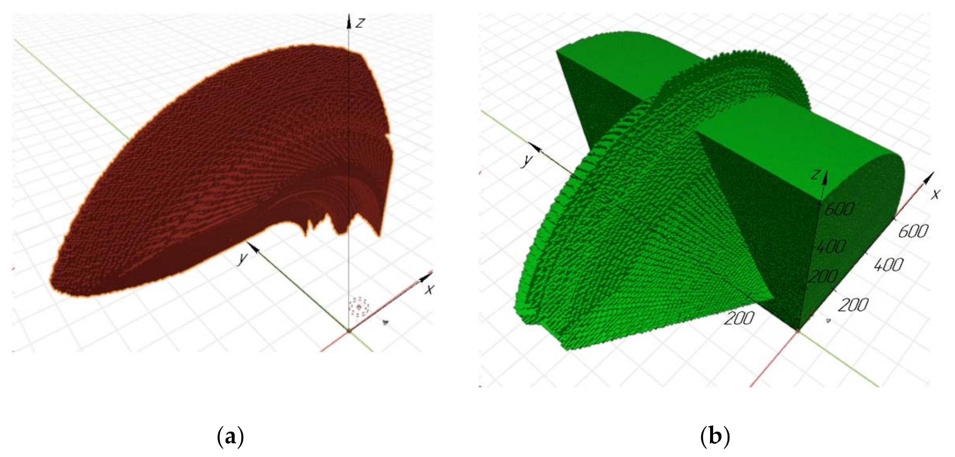
Let us define the workspace of the parallel manipulator, taking into account the rotation of the platform. The range of the angle of the rotary part of the platform $\phi \in \left[0°;90°\right]$ was selected with a step of $2°$ for simulation. The results are shown in Figure 9a. The volume of the workspace due to the rotation of the platform increased from $5.71\times {10}^{-6}$ to $62.04\times {10}^{-6}$ m³. The workspace shows the many achievable end effector positions. However, to avoid collisions of the manipulator with external objects, it is necessary to determine the technological area, that is, the area of possible positions of all intermediate links. So, in addition to the coordinates of the end effector, an iterative discrete determination of the coordinates of points lying on the axes of all links and the moving platform has been added. The discrete step value does not exceed the approximation accuracy. The results in an approximation accuracy of $\delta =5$ mm, as shown in Figure 9b.

7. Defining the Workspace of a Serial Manipulator

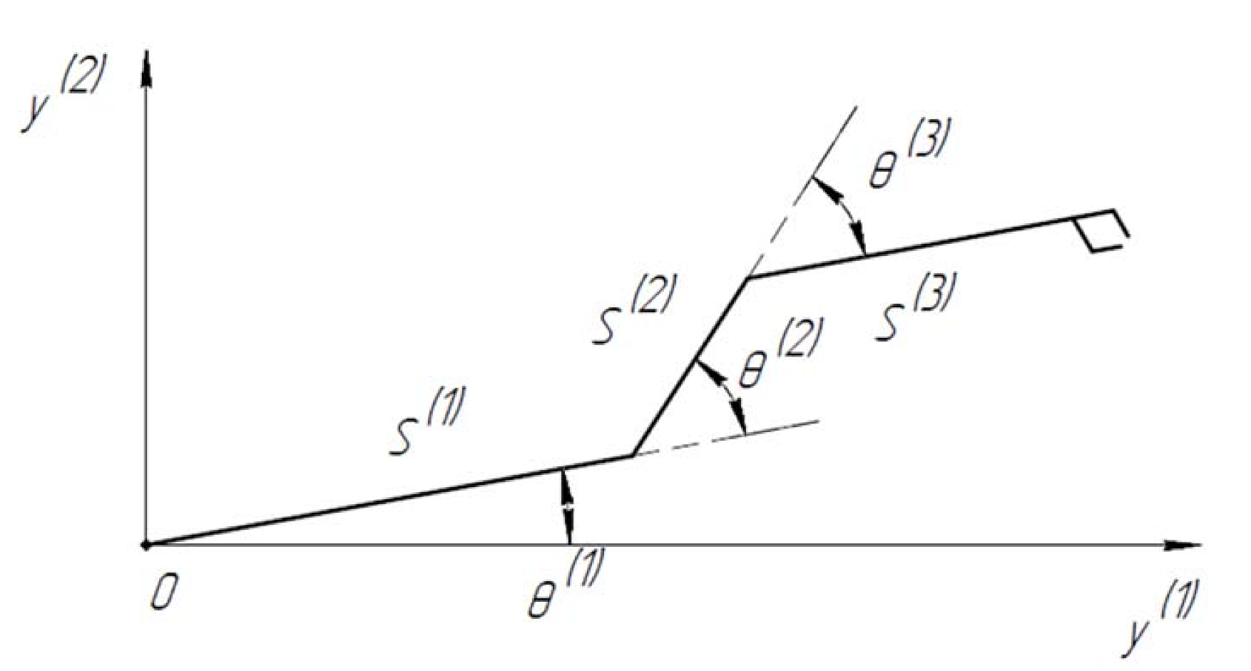
Consider a serial three-link robot (Figure 10). The gripper position is completely determined by the vector of link lengths $s=\left(s^{\left(1\right)},\dots ,s^{\left(k\right)}\right)$ and by the vector of angles $\theta =\left({\theta }^{\left(1\right)},\dots ,{\theta }^{\left(k\right)}\right)$ between the corresponding links. The task of determining the workspace for this work is considered in other works [24,25]. Here is a brief description of the proposed solution.

The permissible set of angles and lengths of links is a box

$$\mathrm{X}=\left[\underset{¯}{s^{\left(1\right)}},\overline{s^{\left(1\right)}}\right]\times \dots \times \left[\underset{¯}{s^{\left(k\right)}},\overline{s^{\left(k\right)}}\right]\times \left[\underset{¯}{{\theta }^{\left(1\right)}},\overline{{\theta }^{\left(1\right)}}\right]\times \dots \times \left[\underset{¯}{{\theta }^{\left(k\right)}},\overline{{\theta }^{\left(k\right)}}\right]$$

(53)

where $\left[\underset{¯}{s^{\left(i\right)}},\overline{s^{\left(i\right)}}\right]$ and $\left[\underset{¯}{{\theta }^{\left(i\right)}},\overline{{\theta }^{\left(i\right)}}\right]$ are given ranges of possible values of the link length $s_i$ and angle ${\theta }_i$, respectively.

The workspace of the robot manipulator is the image $Y=F\left(X\right)$ of the admissible set $X$, where $F\left(s,\theta \right)=\left(f^{\left(1\right)}\left(s,\theta \right),f^{\left(2\right)}\left(s,\theta \right)\right)$ is given by formulas

$$f^{\left(1\right)}\left(s,\theta \right)={{\displaystyle \sum }}_{i=1}^k{s}^{\left(i\right)}·\cos \left({{\displaystyle \sum }}_{j=1}^i{\theta }^{\left(j\right)}\right)$$

(54)

$$f^{\left(2\right)}\left(s,\theta \right)={{\displaystyle \sum }}_{i=1}^k{s}^{\left(i\right)}·\sin \left({{\displaystyle \sum }}_{j=1}^i{\theta }^{\left(j\right)}\right)$$

(55)

During the operation of the algorithm for determining the workspace of the serial mechanism, a list of points from the set X is maintained such that its image F, which is determined using (54) and (55), contains a finite set of pairwise incomparable points, which after the completion of the algorithm will be an ε-approximation of the boundary of the set Y. An algorithm for constructing an ε-Pareto set with guaranteed accuracy ε is given in [26].

In the current work, the covering set has been transformed into an ordered set of integers, similarly to the transformation of the covering set of a tripod. In this case, the vector has a two-level structure, since the workspace of a serial robot is two-dimensional.

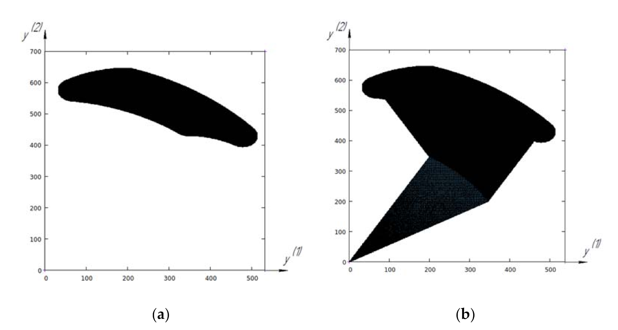
Figure 11a shows the simulation results for the following dimensions $—s_1=400$, $s_2=265$, $s_3=35$, ranges of angles: ${\theta }_1\in \left[\frac{\pi }{6},\frac{\pi }{3}\right], {\theta }_2\in \left[\frac{\pi }{6},\frac{\pi }{3}\right], {\theta }_3\in \left[-\pi ,\pi \right]$.

The technological area was similarly defined for a serial manipulator. The results are shown in Figure 11b.

8. Determination of Links Interference of a Multi-Robotic System

In the process of collaborative execution of tasks by a multi-robotic system, two problems arise within the framework of determining a possible intersection of links. The first task is to determine the presence of intersections for the given positions of each of the manipulators. Each of the positions can be obtained by discretizing the trajectory while performing the operation, taking into account the time. The second task is to determine the presence of intersections, taking into account all achievable positions of the manipulators for a given relative position of the mobile platforms.

To solve the first problem, we use the approach to determining the intersections of links, described in Section 3. In this case, the intersection of all combinations of manipulator links with each other is checked. The coordinates specify the mutual position of the platforms $x_s$ and $y_s$ by the angle λ of rotation of the coordinate system of the mobile platform of the serial manipulator relative to the coordinate system of the parallel manipulator. Checking the intersection of the links of the serial manipulator with the rotating platform of the parallel manipulator includes turning relative to the X axis by an angle at which the plane of the turntable coincides with the XOY plane. In this case, checking is reduced to determine the intersections of the links of the serial manipulator with rectangles parallel to the XOY, XOZ and YOZ planes.

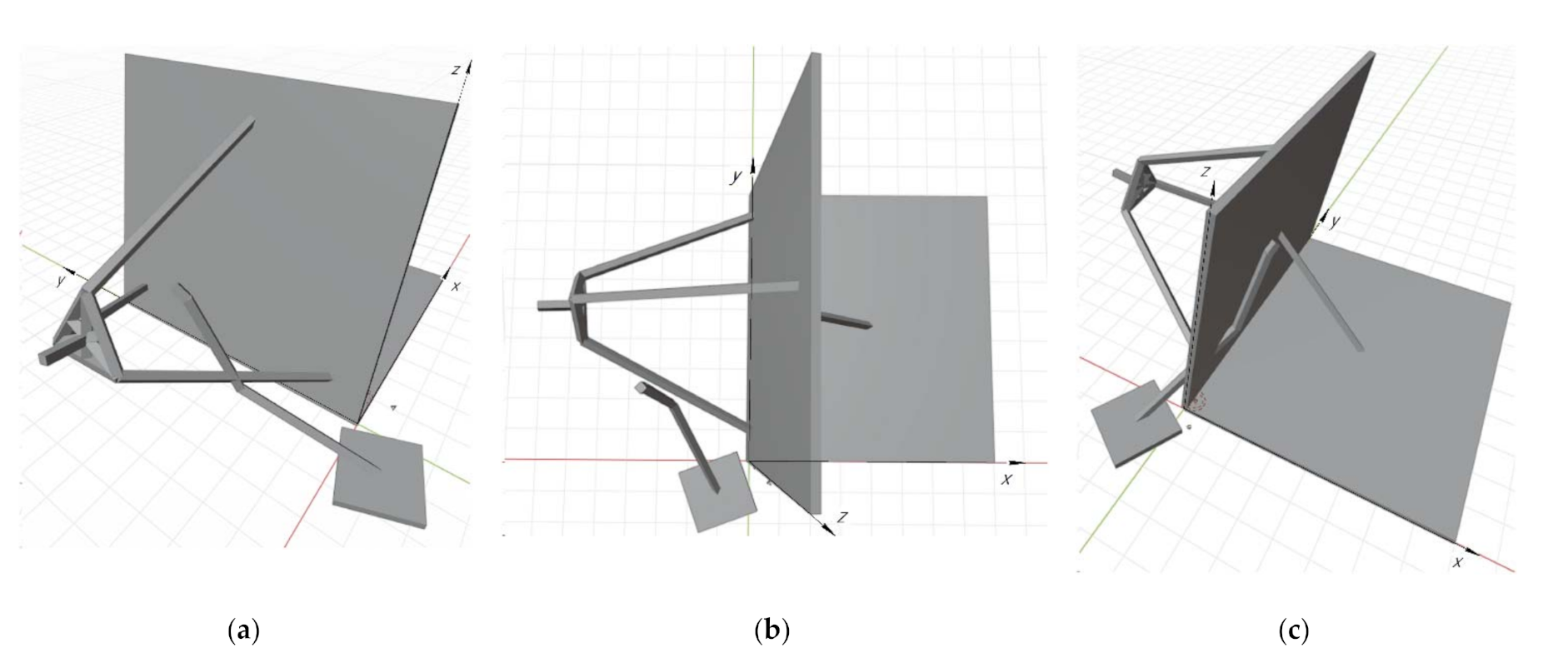
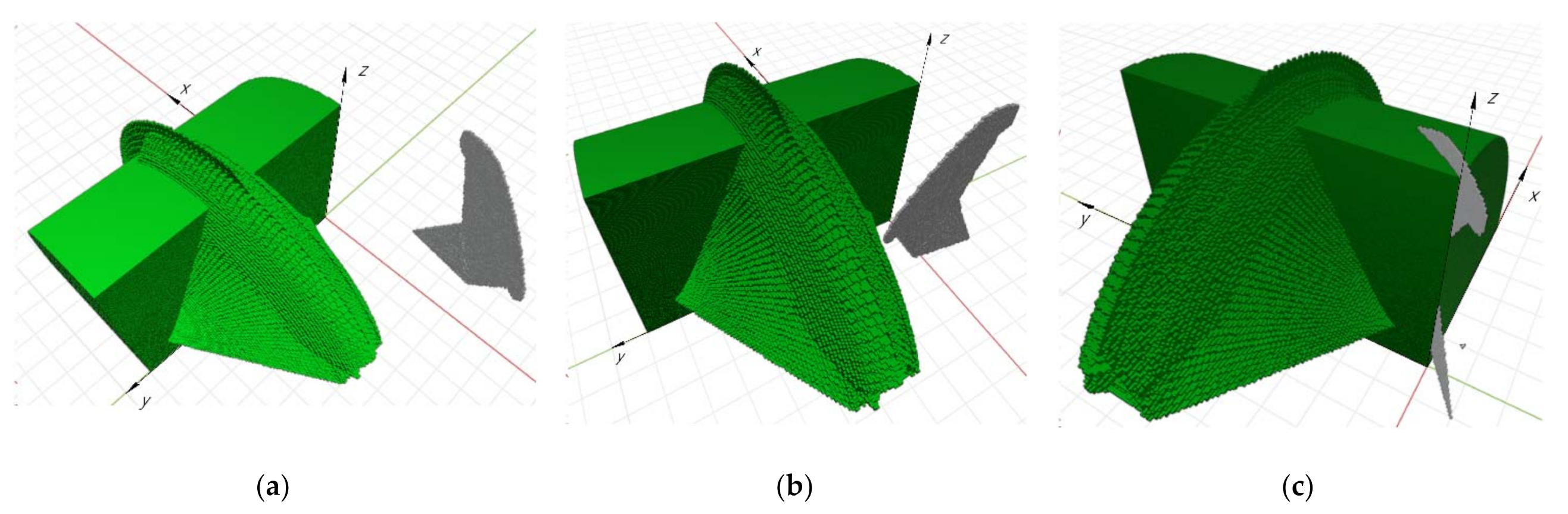
Simulation was performed for $x_s=-100$ mm, $y_s=-100$ mm, $\theta =\psi =0°$, $z_0=500$ mm, $\phi =78°$. In the first case, for $\lambda =110°, {\theta }^{\left(1\right)}=30°, {\theta }^{\left(2\right)}=35°, {\theta }^{\left(3\right)}=-20°$, an intersection was found between the links (Figure 12a), in the second for $\lambda =110°, {\theta }^{\left(1\right)}=40°, {\theta }^{\left(2\right)}=40°, {\theta }^{\left(3\right)}=10°$ there is no intersection (Figure 12b), in the third, for $\lambda =60°, {\theta }^{\left(1\right)}=30°, {\theta }^{\left(2\right)}=35°, {\theta }^{\left(3\right)}=-20°$, an intersection occurs between the link of the serial manipulator and the turntable parallel manipulator (Figure 12c). To verify the results, visualization was implemented through automatic generation of a 3D model of a multi-robotic system for given positions (Figure 12). The results of checking the intersections of the manipulators links coincide with the results of checking using the generated 3D model of the multi-robotic system. The algorithm is fast enough to check about ${10}^6$ different positions per second, which makes it possible to check intersections in real time, discretely checking the trajectories of the manipulators.

To solve the second problem, let us determine the minimum distance between the regions. The distance $\Delta$ between the centers of the boxes included in the technological areas of the manipulators is determined iteratively. The dimensions of the boxes for each of the measurements are equal to the approximation accuracy $\delta$. Therefore, we take into account the distance from the center of the box to the top of the box, which is $\frac{\sqrt{2}\delta }{2}$ for each of the two boxes, between the centers of which we determine the distance. Based on this, we write down the condition for the absence of a possible intersection of the links:

$$\Delta >D_{link}+\sqrt{2}\delta$$

(56)

If the condition is not met for any of the combinations of boxes, the iterative check stops.

Simulation was performed for the following relative positions of mechanisms $—x_s=-300$ mm, $y_s=-200$ mm, $\lambda =150°$ (Figure 13a), $x_s=-200$ mm, $y_s=-200$ mm, $\lambda =100°$ (Figure 13b) and $x_s=-100$ mm, $y_s=-100$ mm, $\lambda =45°$ (Figure 13c). In the first case, there is no intersection of the links. In the second case, the technological areas do not intersect, however, condition (56), which takes into account the thickness of the links, is not met, and therefore a collision of manipulators is possible. In the third case, there are intersections, which confirms the intersection of technological areas. The time for intersection calculating in the absence of intersections was 14 s. In the case of intersections, the computation time can be significantly lower.

9. Discussion

Thus, the solution of two problems is given within the framework of determining the possible intersection of links for the collaborative performance of tasks by a multi-robotic system. The first problem is solved based on the proposed approach to determine the intersections of the manipulator links. The results were verified using visualization by automatically generating a 3D model of a multi-robotic system for given positions. The implemented algorithm for checking the intersections of links has sufficient performance to check about ${10}^6$ different positions of the manipulators per second, which allows checking in real time, discretely checking the trajectories of the manipulators. The second problem is solved by calculating the distance between the technological areas of manipulators. To determine them, the method of nonuniform coverings was used with the subsequent transformation of the results into a partially ordered set of integers.

The proposed approaches can be applied in various areas of the industry. At the same time, they can be modified, taking into account the specifics of the performed operations, the configuration of the robots, as well as the required distances between the robot and other objects. However, depending on these conditions, it is required to conduct a preliminary analysis of the effectiveness of using the proposed approach in comparison with the use of various sensors, which are often used to avoid collisions.

The proposed approach to solving the second problem can be used both to determine a possible collision of manipulators with each other and to localize a collision with external obstacles. In this case, it is required to determine the minimum distance not between the technology areas, but between the technology area and the area occupied by the obstacle. Authors should also list the limitations of the work. For the first problem, the proposed algorithm implies the use of fairly simple geometry for an approximated description of solid bodies. The algorithm can be modified to use more complex geometry, but this will increase the computational complexity. Another limitation is the need to accurately localize the position of the moving platforms. Otherwise, the value of the safe distance between the manipulators must be increased by the error in determining the position of the movable platforms.

The results obtained can be used to solve the problem of control and planning the trajectory of mobile platforms within the framework of a multi-robotic system.

References

- Ferber, J. Multi-Agent Systems an Introduction to Distributed Artificial Intelligence; Addison-Wesley Reading: Boston, MA, USA, 1999; Volume 1. [Google Scholar]
- Eren, T.; Belhumeur, P.N.; Anderson, B.D.; Morse, A.S. A framework for maintaining formations based on rigidity. In Proceedings of the 15th IFAC World Congress, Barcelona, Spain, 21–26 July 2002; pp. 2752–2757. [Google Scholar]
- Olfati-Saber, R.; Murray, R.M. Distributed cooperative control of multiple vehicle formations using structural potential functions. IFAC Proc. Vol. 2002, 15, 242–248. [Google Scholar] [CrossRef] [Green Version]
- Areak, M. Passivity as a design tool for group coordination. In Proceedings of the IEEE American Control Conference, Minneapolis, MN, USA, 14–16 June 2006; p. 6. [Google Scholar] [CrossRef]
- Balch, T.; Arkin, R.C. Behavior-based formation control for multi robot teams. Robotics and Automation. IEEE Trans. 1998, 14, 926–939. [Google Scholar] [CrossRef] [Green Version]
- Lewis, M.A.; Tan, K.-H. High precision formation control of mobile robots using virtual structures. Auton. Robot. 1997, 4, 387–403. [Google Scholar] [CrossRef]
- Desai, J.P.; Ostrowski, J.; Kumar, V. Controlling formations of multiple mobile robots. In Proceedings of the IEEE International Conference on Robotics and Automation, Leuven, Belgium, 20–20 May 1998; Volume 4, pp. 2864–2869. [Google Scholar]
- Sandeep, S.; Fidan, B.; Yu, C. Decentralized cohesive motion control of multi-agent formations. In Proceedings of the 14th Mediterranean Conference on Control and Automation, Ancona, Italy, 28–30 June 2006; pp. 1–6. [Google Scholar] [CrossRef]
- Wang, C.; Xie, G.; Cao, M. Forming circle formations of anonymous mobile agents with order preservation. IEEE Trans. Autom. Control 2013, 58, 3248–3254. [Google Scholar] [CrossRef]
- Alizade, R.I.; Tagiyev, N.R.; Duffy, J. A forward and reverse displacement analysis of an in-parallel spherical manipulator. Mech. Mach. Theory 1994, 29, 125–137. [Google Scholar] [CrossRef]
- Bulca, F.; Angeles, J.; Zsombor-Murray, P.J. On the workspace determination of spherical serial and platform mechanisms. Mech. Mach. Theory 1999, 34, 497–512. [Google Scholar] [CrossRef]
- Clavel, R. Conception D’un Robot Parall‘Ele Rapide ‘A 4 Degr’Es de Libert´E. Ph.D. Thesis, Swiss Federal Institute of Technology Lausanne, Lausanne, Switzerland, 1991. [Google Scholar]
- Husty, M.L. On the workspace of planar three-legged platforms. In Proceedings of the World Automation Congress, Montpellier, France, 28–30 May 1996; Volume 3, pp. 339–344. [Google Scholar]
- Merlet, J.P. Interval Analysis and Robotics. In Robotics Research; Kaneko, M., Nakamura, Y., Eds.; Springer: Berlin/Heidelberg, Germany, 2010; Volume 66. [Google Scholar] [CrossRef] [Green Version]
- Khalilpour, S.; Zarif Loloei, A.; Taghirad, H.; Tale Masouleh, M. Feasible Kinematic Sensitivity in Cable Robots Based on Interval Analysis. In Cable-Driven Parallel Robots; Springer: Berlin/Heidelberg, Germany, 2012; pp. 233–249. [Google Scholar]
- Merlet, J.P. Determination of 6D Workspace of Gough-Type Parallel Manipulator and Comparison between Different Geometries. Int. J. Robot. Res. 1999, 18, 902–916. [Google Scholar] [CrossRef]
- Evtushenko, Y.; Posypkin, M.; Rybak, L.; Turkin, A. Approximating a solution set of nonlinear inequalities. J. Glob. Optim. 2018, 71, 129–145. [Google Scholar] [CrossRef]
- Malyshev, D.; Posypkin, M.; Rybak, L.; Usov, A. Approaches to the Determination of the Working Area of Parallel Robots and the Analysis of Their Geometric Characteristics. Eng. Trans. 2019, 67, 333–345. [Google Scholar] [CrossRef]
- Malyshev, D.; Rybak, L.; Behera, L.; Mohan, S. Workspace Modelling of a Parallel Robot with Relative Manipulation Mechanisms Based on Optimization Methods. In Robotics and Mechatronics; Kuo, C.H., Lin, P.C., Essomba, T., Chen, G.C., Eds.; ISRM 2019; Mechanisms and Machine Science, Springer: Cham, Switzerland, 2020; Volume 78. [Google Scholar]
- Rao, P.S.; Rao, N.M. Position Analysis of Spatial 3-RPS Parallel Manipulator. Int. J. Mech. Eng. Robot. Res. 2013, 2, 80–90. [Google Scholar]
- Gosselin, C.; Angeles, J. Singularity analysis of closed-loop kinematic chains. IEEE Trans. Robot. Autom. 1990, 6, 281–290. [Google Scholar] [CrossRef]
- Anvari, Z.; Ataei, P.; Masouleh, M.T. The collision-free workspace of the tripteron parallel robot based on a geometrical approach. In Computational Kinematics; Springer: Berlin/Heidelberg, Germany, 2018; pp. 357–364. [Google Scholar] [CrossRef]
- Malyshev, D.I.; Posypkin, M.A.; Gorchakov, A.Y.; Ignatov, A.D. Parallel algorithm for approximating the work space of a robot. Int. J. Open Inf. Technol. 2019, 7, 1–7. [Google Scholar]
- Posypkin, M.A. Metody Global’noj I Mnogokriterial’noj Optimizacii na Baze Koncepcij Vetvej i Granic i Neravnomernyh Pokrytij [Global and Multicriteria Optimization Methods Based on the Concepts of Branch and Bounds and Non-Uniform Coving]. Ph.D. Thesis, Dorodnitsyn Computing Center, Federal Research Center “Computer Science and Control”, Russian Academy of Sciences, Moscow, Russia, 2014. [Google Scholar]
- Rybak, L.A.; Behera, L.; Malyshev, D.I.; Virabyan, L.G. Approximation of the workspace of parallel and serial structure manipulators as part of the multi-robot system. Bull. BSTU Named V.G. Shukhov. 2019, 8, 121–128. [Google Scholar] [CrossRef]
- Evtushenko, Y.G.; Posypkin, M.A. Nonuniform covering method as applied to multicriteria optimization problems with guaranteed accuracy. Comput. Math. Math. Phys. 2013, 53, 144–157. [Google Scholar] [CrossRef]
Figure 1.
Diagram of a multi-robotic system—(a) serial manipulator, (b) parallel manipulator.
Figure 2.
Parallel manipulator—(a) without a movable base, (b) on a movable base.
Figure 3.
Representation of the links of the mechanism.
Figure 4.
Checking the intersection of links for case 1—(a) for , (b) for .
Figure 5.
Checking the intersection of links for case 2 —(a) no intersection for , (b) no intersection for , (c) intersection for , (d) intersection for .
Figure 6.
Workspace of the parallel manipulator—(a)—for the range of angles and , (b)—for the range of angles and .
Figure 7.
Examples of link intersections for the range of angles and —(a) intersection of links and , and , (b) intersection of links and , and .
Figure 8.
Workspace of the parallel manipulator—(a)—with a negative sign of the determinant of the Jacobi matrix, (b)—with a positive sign.
Figure 9.
Serial manipulator areas—(a) workspace, (b) technological area.
Figure 10.
Angles and links defining the configuration of the robotic arm.
Figure 11.
Serial manipulator areas: (a) workspace, (b) technological space.
Figure 12.
Relative position of the multi-robotic system—(a) the presence of an intersection between the links of the manipulators, (b) the absence of intersections, (c) the intersection of the serial manipulator with the rotating platform of the parallel manipulator.
Figure 13.
Relative position of technological areas of manipulators—(a) absence of intersections, (b) presence of collisions of links without intersection of technological areas, (c) presence of intersections.
Publisher’s Note: MDPI stays neutral with regard to jurisdictional claims in published maps and institutional affiliations. |
© 2021 by the authors. Licensee MDPI, Basel, Switzerland. This article is an open access article distributed under the terms and conditions of the Creative Commons Attribution (CC BY) license (https://creativecommons.org/licenses/by/4.0/).
Share and Cite
MDPI and ACS Style
Behera, L.; Rybak, L.; Malyshev, D.; Gaponenko, E. Determination of Workspaces and Intersections of Robot Links in a Multi-Robotic System for Trajectory Planning. Appl. Sci. 2021, 11, 4961. https://doi.org/10.3390/app11114961
AMA Style
Behera L, Rybak L, Malyshev D, Gaponenko E. Determination of Workspaces and Intersections of Robot Links in a Multi-Robotic System for Trajectory Planning. Applied Sciences. 2021; 11(11):4961. https://doi.org/10.3390/app11114961
Chicago/Turabian StyleBehera, Laxmidhar, Larisa Rybak, Dmitry Malyshev, and Elena Gaponenko. 2021. "Determination of Workspaces and Intersections of Robot Links in a Multi-Robotic System for Trajectory Planning" Applied Sciences 11, no. 11: 4961. https://doi.org/10.3390/app11114961
Note that from the first issue of 2016, this journal uses article numbers instead of page numbers. See further details here.