Data Enhancement for Plant Disease Classification Using Generated Lesions

Abstract

Deep learning has recently shown promising results in plant lesion recognition. However, a deep learning network requires a large amount of data for training, but because some plant lesion data is difficult to obtain and very similar in structure, we must generate complete plant lesion leaf images to augment the dataset. To solve this problem, this paper proposes a method to generate complete and scarce plant lesion leaf images to improve the recognition accuracy of the classification network. The advantages of our study include: (i) proposing a binary generator network to solve the problem of how a generative adversarial network (GAN) generates a lesion image with a specific shape and (ii) using the edge-smoothing and image pyramid algorithm to solve the problem that occurs when synthesizing a complete lesion leaf image where the synthetic edge pixels are different and the network output size is fixed but the real lesion size is random. Compared with the recognition accuracy of human experts and AlexNet, it was shown that our method can effectively expand the plant lesion dataset and improve the recognition accuracy of a classification network.

1. Introduction

Plant diseases have led to a significant decline in the production and quantity of crops worldwide [1]. A series of plant diseases, such as citrus canker [2], have caused billions of dollars in losses each year. In more severe cases, it has even led to the extinction of species; for example, Panama disease led to the extinction of the Gros Michel banana [3]. Currently, many plant diseases cannot be cured and can only be dealt with when they are detected. Plant diseases usually produce corresponding lesions; however, due to the complexity and diversity of diseases, the lesions are often identified by experts. Great economic loss is caused because these diseases cannot be treated early. If these diseases can be accurately identified and treated early, the economic losses will be greatly reduced and ecological disasters caused by disease transmission can be avoided.

Traditional computer vision techniques seek to program a model that can identify a series of traits empirically. However, many plant lesion structures are complex and similar, and their colors are diverse, which makes the diagnosis of plant lesions difficult. Recently, machine learning and especially convolutional neural network models have exhibited considerable strengths for image recognition applications. However, most deep learning algorithms are too complex in network structures and require a large training set. For many plant lesion classification applications, the training instances and related data are scarce. Novel models and algorithms are in high demand that can utilize the scarcity of training images to yield a good recognition accuracy.

Since Goodfellow et al. [4] proposed the generative adversarial network (GAN), the generated image quality has greatly improved. When a GAN is used to generate plant lesion images, generating the complete lesion leaf images directly will generate images with a very poor quality (see Appendix A, Figure A1, Table A1) due to the complexity of the lesion structures. We cropped the lesion area of the leaf image and generated the lesion images with a higher subjective effect. However, many plant lesions have similar structures, such as plant cankers caused by Pseudomonas, like citrus canker [2] and pitaya canker [5] (Figure 1). When only the lesion information is used, the classification network cannot accurately identify the lesion. It is necessary to use the lesion information and the leaf information to accurately identify the corresponding disease types (see Appendix A, Table A2). In order to solve the problem, many plant diseases require the lesion and leaf information to be accurately identified, but a GAN cannot generate a complete plant leaf image with a good quality. We propose a binarization plant lesion generation method that uses a binarization generator network with image edge smoothing (ES-BGNet).

Figure 1. Images of different leaves with similar lesion structures: (a) citrus canker and (b) pitaya canker. If there is no leaf information, it is difficult to distinguish the type of lesion.

Our approach includes multiple steps:

(i)

We first input the binarized image and cropped lesion images into a GAN to generate plant lesions with a specific shape. Meanwhile, we also introduced the dropout layer of the network [6] to solve the problem of image overfitting and improve the training speed.

(ii)

We used the image pyramid [7] and the image edge smoothing algorithm [8] to solve the problem regarding synthesizing a complete lesion leaf image where the synthetic edge pixels are different and the network output size is fixed, but the real lesion size is random.

2. Related Work

Recently, various researches have focused on the problem of plant lesions. Zhang et al. [9] identified citrus canker with a two-level hierarchical detection structure based on global and local features. Zhongliang et al. [10] analyzed rapeseed lesions and extracted parameters with a threshold-based image processing technique. Al-Tarawneh et al. [11] used image segmentation and C-means classification to identify olive leaf spot. Sunny et al. [12] used histogram-enhanced support vector machines to identify citrus cankers. Singh et al. [13] used a support vector machine to identify fungal rust in peas.

Models that apply deep learning techniques had not been introduced until recently due to the lack of computational power. Most of the latest approaches that have been proven to be efficient relied on a neural network to identify plant features that are highly intractable by the usual methods. Reyes et al. [14] used a neural network to identify 1000 different plant features. Tan et al. [15] used deep learning to identify the spotted melon lesion. Sladojevic et al. [16] proposed a method for using deep learning to identify plant diseases. Toda et al. [17] identified lesion data with a convolutional neural network in PlantVillage. Bera et al. [18] identified rice diseases with deep learning. Minaee et al. [19] surveyed the strengths and potentials of deep learning for biometric recognition. Brahimi et al. [20] proposed a new trainable visualization method for plant disease classification based on a convolutional neural network (CNN) architecture composed of two deep classifiers. Francis et al. [21] created and developed a convolutional neural network model to perform plant disease detection and classification using apple and tomato leaf images of healthy and diseased plants. Nestsiarenia et al. [22] solved the problem of the detection and prevention of diseases in agricultural crops by using machine learning techniques. Their research showed that deep learning has great potential in plant lesion recognition.

Apart from the convolutional neural network (CNN), another major development in deep learning is the development of GAN, which was first proposed by Goodfellow et al. [4]. The generator network maps a source of noise to the input space. The discriminator network receives either a generated sample or a true data sample and must distinguish both. The generator is trained to fool the discriminator. In order to make a GAN more applicable, Deep Convolutional GAN (DCGAN) [23] combined a CNN with a GAN. Wasserstein GAN (WGAN) [24] solved the problem of GAN training instability by introducing a Wasserstein distance. Improved Wasserstein GAN (WGAN-GP) [25] offered an alternative to WGAN weight cropping, which solves the problem of unstable WGAN training. Least Squares GAN (LSGAN) [26] used the mean square loss to replace the logarithmic loss and solved the problem of unstable GAN training. Progressive GAN [27] stabilized the training to generate better images by using the gradual increase of the Laplacian pyramid in a GAN [28]. Giuffrida et al. [29] showed that artificial images can be used to augment the training data, thus reducing the absolute difference in counting error by 5.4% for leaf counting. Zheng et al. [30] proposed the label smoothing regularization for outliers (LSRO) that uses a DCGAN to generate unlabeled samples. Conditional GANs (cGANs) [31] offers a new projection-based approach that improves the image generation. Conditional Infilling GAN (CiGAN) [32] uses a binarized image and background leaves to generate a breast X-ray film sample with good results. Zhu et al. [33] used a conditional GAN setup to create artificial images of Arabidopsis plants, with the focus on the improvement of leaf counting. Purbaya et al. [34] used a GAN to synthesize leaf images and improve regularization. Ward et al. [35] used generated images to augment the training set and improved the accuracy of leaf-image segmentation. Zhang et al. [36] used spectrum normalization to improve the effect of GAN training. Dong et al. [37] employed the sigmoid-adjusted straight-through estimators to estimate the gradients for the binary neurons and train the whole network by end-to-end backpropagation. Song et al. [38] used binary GANs to embed images into binary code and generate images similar to the original image. Chen X et al. [39] used the attention mechanism to improve the quality of wild images. Minaee et al. [40] used the attention mechanism to enable the network to focus on important parts of the face, improving the accuracy of facial expression recognition. Sapoukhina et al. [41] used a GAN to convert RGB images to grayscale images to boost the performance for the leaf segmentation of Arabidopsis thaliana in chlorophyll fluorescent imaging without any manual annotation. Kuznichov et al. [42] used the generated rose plant leaf image to expand the training set to improve the accuracy of the segmentation network. Zhang et al. [43] used a DCGAN to generate citrus canker images to improve the accuracy of the classification network. Lucic et al. [44] used fewer labels to generate a better Fréchet inception distance (FID) image. Chen et al. [45] used adversarial training and self-supervision to make fully unsupervised learning become scaled to attain an FID of 23.4 on unconditional ImageNet generation. Tran et al. [46] applied self-supervised learning via the geometric transformation on input images and assigned the pseudo-labels to these transformed images to improve an unconditional GAN. Lin et al. [47] produced images that were larger than training samples by combining them with the originally generated full image. Takano et al. [48] explored how selecting a dataset affects the outcome by using three different datasets to see that a Super-Resolution GAN (SRGAN) fundamentally learns objects, and using their shape, color, and texture, redraws them in the output rather than merely attempting to sharpen edges. Zhang D et al. [49] gradually increased the difficulty of the discriminator by progressively augmenting its input or feature space, thus enabling continuous learning of the generator, leading to a better performance.

In this study, we refer to the comparison of a GAN evaluation in Lucic et al. [50], and we build the model of the generator network using a WGAN-GP and CiGAN as a base. Compared with the algorithm that uses the binarized image in the reference, our advantage was using the binarized image to generate a lesion image with a specific shape. It solved the problem that occurs when the random-shaped lesions are synthesized with the leaves, and so the lesions must be marked. However, due to the complexity of the lesion structures, it is difficult to mark the lesions completely using the algorithm, and manual marking needs a lot of time and money.

3. Methods

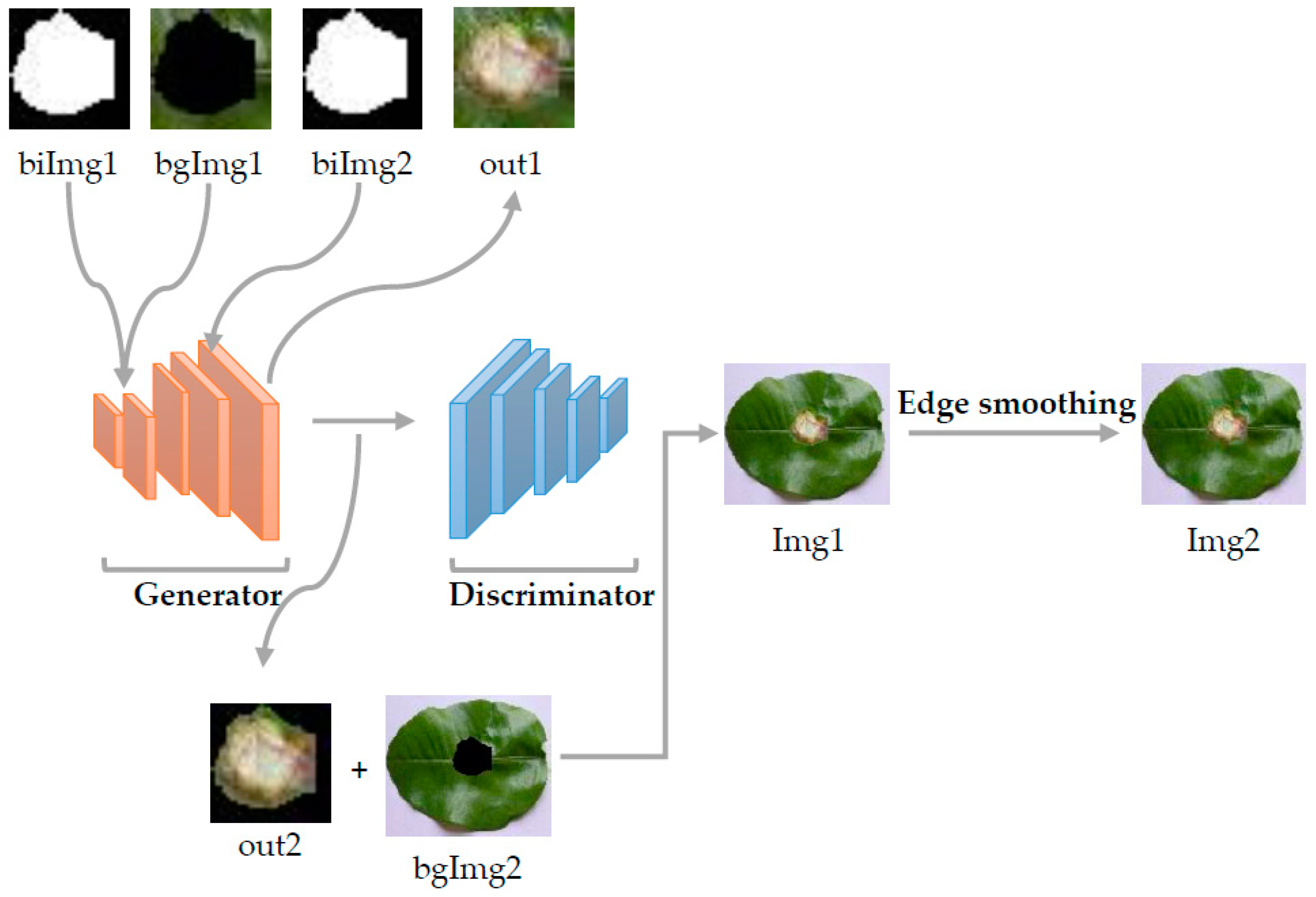
3.1. Network Architecture

Our network architecture is shown in Figure 2. The input of the generator was a set of Gaussian distribution data. After a convolution, the result of the first convolution was multiplied by the lesion binarized image biImg1, and the multiplied result was then added to the marked leaf image bgImg1. After three more convolutions, the resulting lesion out1 is output to the discriminator. At the same time, the output out1 was multiplied by the binarized lesion image to obtain the out2 lesion image. We then synthesized out2 and the marked leaf image bgImg2, and our desired result Img2 was obtained via edge smoothing the obtained Img1.

Figure 2. Architecture of our generator network. We had a total of five convolutional layers, where bgImg1 (8 × 8 × 3) and bgImg2 (256 × 256 × 3) were binarized marked leaf images, biImg1 (8 × 8 × 1) and biImg2 (64 × 64 × 1) were different sizes of the same binarized image. out1 (64 × 64 × 3) was the generated lesion image trained with the discriminator, and out2 (64 × 64 × 3) was the area of the lesion after binarization. Img1 was an image synthesized by out2 and bgImg2, and Img2 (256 × 256 × 3) was an image after the Img1 (256 × 256 × 3) edge smoothing.

Due to the uniform size of the images generated by the GAN, the size of the plant lesion and the lesion’s relative position on the leaves in the natural environment were completely random. In order to make the generated image more in line with the real lesion, we obtained lesion images of different sizes by placing the generated lesion image at different positions of the leaf and using the image pyramid.

3.2. ES-BGNet

We proposed a generation net to solve the problem of insufficient leaf lesions data. The GAN training strategy is to define a game between two competing networks. The generator network maps a source of noise to the input space. The discriminator network receives either a generated sample or a true data sample, both of which must be distinguished. The generator is trained to fool the discriminator.

The loss of our generator is:

$$L_{\mathrm{G}}=\min \left(-D\left(g\left(z\right)\right)\right).$$

(1)

The loss of our discriminator is:

$$L_D=\min \left(\begin{array}{c}\mathbb{E}\\ \tilde{x}~{\mathbb{P}}_g\end{array}\left[D\left(\tilde{x}\right)\right]-\begin{array}{c}\mathbb{E}\\ x~{\mathbb{P}}_r\end{array}\left[D\left(x\right)\right]+\lambda \begin{array}{c}\mathbb{E}\\ \widehat{x}~{\mathbb{P}}_{\widehat{x}}\end{array}[{(|\left|{\nabla }_{\widehat{x}}D\left(\widehat{x}\right)\right|{|}_2-1)}^2]\right),$$

(2)

where $x$ is the real sample image; $\tilde{x}$ is a fake image generated by the $g\left(z\right)$ generator; ${\mathbb{P}}_r$ is the distribution of real data; ${\mathbb{P}}_g$ is x = $G$($z$); $z$ is a set of Gaussian distribution data; $\widehat{x}=ϵx+\left(1-ϵ\right)\tilde{x}$; $ϵ$ is a random value obeying $U\left[0,1\right]$; and $\lambda$ is the penalty coefficient, for which we use $\lambda =10$. Meanwhile, our generator trained once every iteration, while the corresponding discriminator trained five times. Our learning rate was 0.0001; optimization was performed using the Adam optimization algorithm.

3.3. Image Marker Layer

We added an image marker layer to the generator network using the image binarization algorithm. For the algorithm’s selection of the binarized plant lesion image, we compared Iterative Self-Organizing Data Analysis Technique (ISODATA) [51], the histogram-based threshold algorithm analysis [52], and the image binarization through image filtering and histograms [53], which are found in Table A4 of Appendix A. Because the number of samples was too small to train the segmentation network, the lesion and leaf area pixel value of the plant lesion image had a more obvious bimodal trend. Therefore, a threshold-based histogram bimodal algorithm [52] was adopted to generate a binarized image of the original dataset.

We created a histogram of the pixel values of the grayscale image of the lesion image with 20-pixel intervals:

$$nu{m}_{type}=number\left(p_i\right);$$

(3)

then, we calculated the slope of the corresponding pixel according to the histogram:

$$k_{type}=\frac{\left(nu{m}_{type}-nu{m}_{type-1}\right)}{20},$$

(4)

and the threshold we calculated was:

$$threshold=\frac{to{p}_i+to{p}_j}{2},$$

(5)

where $p_i$ is the value of the ith pixel, $type=\left[\frac{p_i}{20}\right]$, $nu{m}_{type}$ is the number of pixels corresponding to $type$, and $k_{type}$ is the left slope corresponding to the pixel where $k_{type=0}=0$. Further, $thres$ is the threshold we calculated, and $to{p}_i$ and $to{p}_j$ are the values of the two peak pixels corresponding to the histogram.

3.4. Image Edge Weighted Smoothing

When we combined the generated lesions with the leaves, the edge pixels of some of the image synthesis regions were quite different. Comparing the commonly used edge smoothing algorithms, such as the mean filtering and median filtering [54], Gaussian filtering [55], and gradient-based image filtering [56] through experimentation (in Table A6 of Appendix A), we chose [54] image edge weighted smoothing filtering:

$$p_i=\lambda p_i+\left(1-\lambda \right)p_j,$$

(6)

where $p_i$ is the pixel we filtered, $p_j$ is the pixel of the background leaf adjacent to pixel $p_i$, and $\lambda$ is the weight. We chose $\lambda =0.2$ as our weight through experimental comparison. Our evaluation indicators were the inception score (IS) and the Fréchet inception distance (FID), as shown in Table A8 of Appendix A.

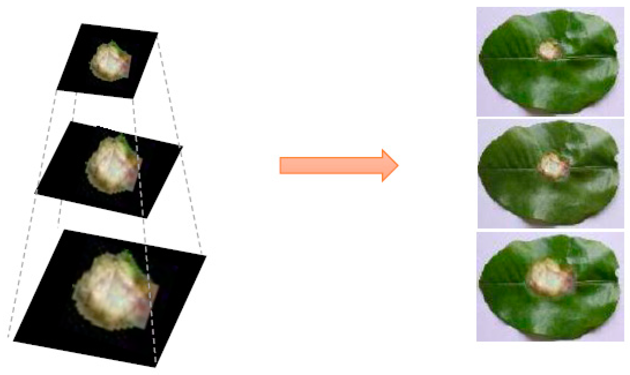
3.5. Bilinear Interpolation Image Pyramid

We found that due to the complex structure of the lesion itself, the lesion characteristics would be lost if the image had too few pixels. By comparing bilinear interpolation [57], nearest neighbor interpolation [58], and bicubic interpolation [59], as shown in Table A10 of Appendix A, we used bilinear interpolation [57] to scale the image to form the structure of the image pyramid. A bilinear map is a function combining elements of two vector spaces to yield an element of a third vector space, and is linear in each of its arguments. In Figure 3, we can work out the position coordinates and pixels of points 1–4 to calculate the position coordinates and pixels of point 5:

$$\frac{p_i-p_j}{x_i-x_j}= \frac{p_i-p}{x_i-x}.$$

(7)

Figure 3. Bilinear interpolation, where points 1–4 are known points and the coordinates and pixel values of point 5 are calculated.

In the image, the difference in coordinate values between adjacent pixels is 1:

$$x_i-x_j=1,$$

(8)

$$p=p_i-\left(p_i-p_j\right)\left(x_i-x\right).$$

(9)

The pixels of point $m$, point $n$, and our target point 5 can be calculated using the above formula, and the position of point 5 can be used as follows:

$$SrcX=\left(dstX\right)\left(\frac{srcWidth}{dstWidth}\right),$$

(10)

$$SrcY=\left(dstY\right)\left(\frac{srcHeight}{dstHeight}\right).$$

(11)

The position information of m and n is:

$$x_m=x_n=x_5,$$

(12)

$$y_m=y_1=y_2,$$

(13)

$$y_n=y_3=y_4$$

(14)

The pixel in the upper-left corner of the image is considered the origin of the coordinate system, $p_i$ and $p_j$ are known pixels, $p$ is the pixel to be calculated, $x_i$ and $x_j$ are positional information of known pixels, and $x$ is the position information to be calculated, $dstX$ is the horizontal axis position information of the scaled image and $dstY$ is the vertical axis position information of the scaled image, $SrcX$ is the horizontal axis position information corresponding to $dstX$ before image scaling and $SrcY$ is the vertical axis position information corresponding to $dstY$ before image scaling, $dstWidth$ is the width of the image in the scaled image and $dstHeight$ is the height of the image in the scaled image, and $srcWidth$ is the width of the image before scaling image and $srcHeight$ is the height of the image before scaling image.

4. Experiments

4.1. Dataset

In the experiment, we shot the citrus canker sample dataset using a Nikon D7500. It was found through experiments that the result of a GAN generating a complete plant lesion leaf image was very bad. We cut the leaf lesion area and generated good cropped lesion images. Then, we used edge smoothing and an image pyramid to synthesize lesions and leaves to obtain complete leaf lesion images. Our source code is available at https://github.com/Ronzhen/ES-BGNet. Our method took 46 h to train on a GTX1070 Ti.

Citrus canker: As is shown in Figure 4, we cut 788 images of the citrus canker dataset and rotated them every 90 degrees. The resulting image of 3152 citrus canker images was taken as our lesion samples. The citrus canker dataset was divided into three categories: 2000 training images, 652 test images, and 500 validation images.

Figure 4. Lesion cut from real lesion leaf images in a citrus canker dataset.

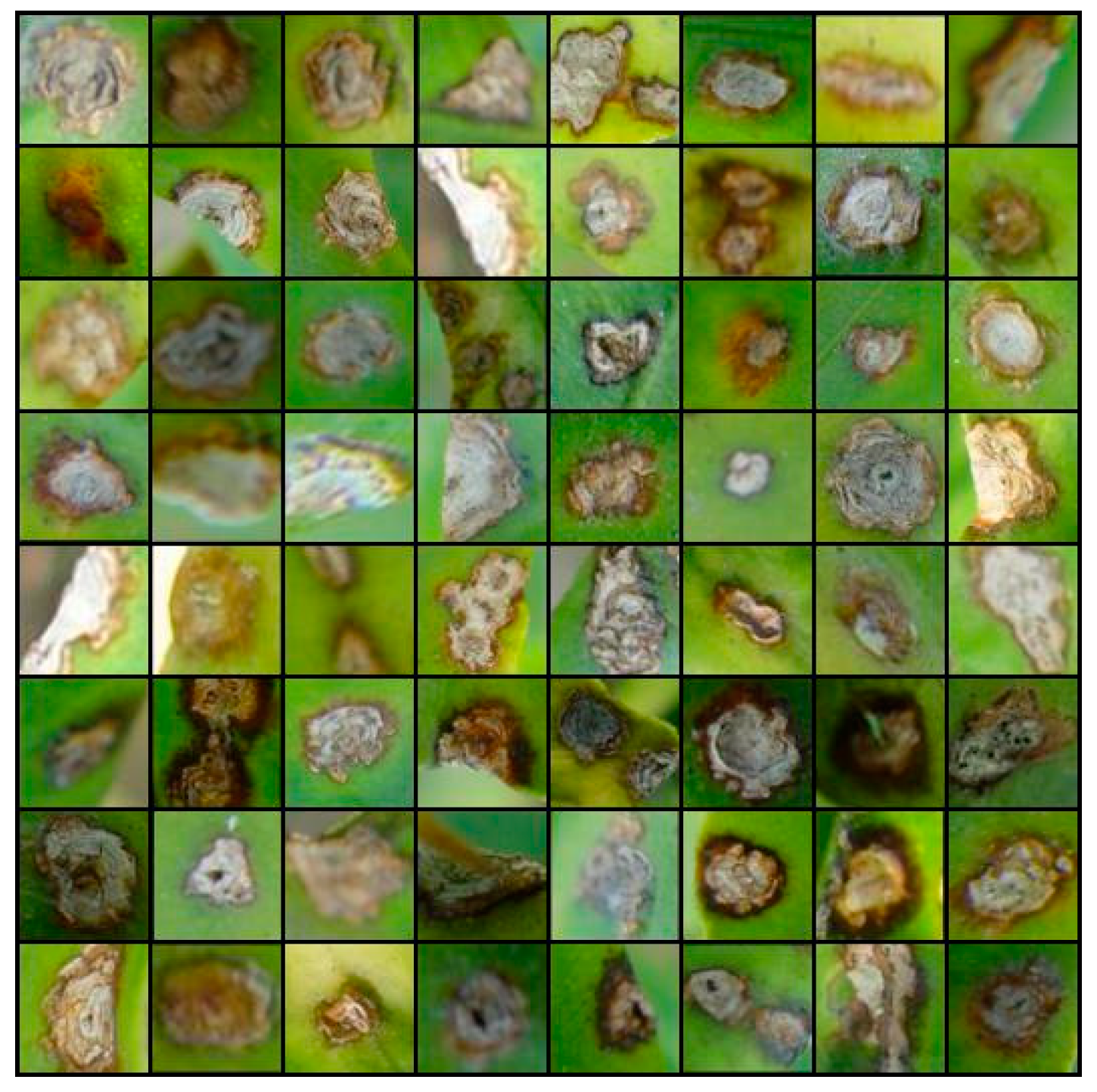
4.2. The Generated Image from ES-BGNet

Figure 5 shows the generated lesion image and the binarized lesion image in the citrus canker dataset. It was apparent that our method generated many lesion images with a special shape.

Figure 5. Images of citrus canker lesions generated using our method: (a) generated citrus canker and (b) citrus canker after binarization.

As is shown in Figure 6, when the generated lesion was synthesized with the leaf, the pixels at the synthetic edge were different. We used a weighted image-edge-smoothing algorithm to synthesize a better image. Meanwhile, in order to simulate the randomness of the lesions’ positions relative to the leaves in the natural environment, we also placed the lesions at different positions on the leaves.

Figure 6. Comparison of images before and after edges were smoothed. Lesions were placed at different locations on the leaves.

In Figure 7, in order to solve the problem that the generated lesion image size was unique with the actual lesion size being random, we used image pyramids to generate lesions of different sizes to be synthesized with the leaves.

Figure 7. Extension of the sample dataset using image pyramids. We used image pyramids to change the size of the lesion image and synthesize it with the leaves. It greatly expanded the number of diseased leaf samples.

4.3. Quality Assessment of Generated Images

We tested the generated lesion image using human experts and AlexNet to evaluate the generated image quality, see Table 1.

Table 1. Precision, recall, F1 score, and accuracy of human experts and AlexNet for classifying real images and generated images. We gathered statistics for 10 trainings, and the difference was statistically significant (p < 0.05).

Method	Precision	Recall	F1 Score	Accuracy
Human Experts Classifier	0.472 ± 0.091	0.380 ± 0.094	0.421 ± 0.088	0.593 ± 0.129
	0.677 ± 0.054	0.666 ± 0.068	0.671 ± 0.080	0.701 ± 0.050

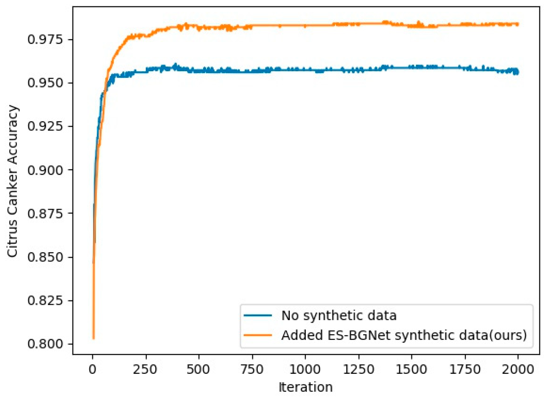
4.4. Compare Accuracy to Determine Whether to Use Synthetic Data in AlexNet

We used AlexNet as a comparison network and compared the recognition accuracy of AlexNet in the same test sets to verify the effectiveness of our method. In order to ensure the unification of the initial weight of the network and reduce the training cost, we used the training model on ImageNet to initialize our AlexNet. We performed 2000 iterations and spent 3 h training Alexnet on a GTX1070 Ti.

As can be seen from Figure 8 and Table 2, using ES-BGNet to expand lesions improved the recognition accuracy of AlexNet. All three methods achieved their best classification accuracy after 500 iterations. This confirmed the effectiveness of our method for extending the deep learning network training sets to improve the recognition accuracy of the classification network.

Figure 8. Contrast through transfer learning. When synthetic data (1000 images) was not used and ES-BGNet synthetic data training (1500 images) was used, we obtained the classification accuracy of AlexNet using the citrus canker dataset.

Table 2. Contrast between not using synthetic data and using edge-smoothing binarization generator network (ES-BGNet) synthetic data to provide the average accuracy of AlexNet using the citrus canker dataset. We gathered the statistics of 10 training exercises, and the difference was statistically significant (p < 0.05).

Dataset	Network	Average Accuracy
Citrus canker	No synthetic data	0.955 ± 0.003
	Added ES-BGNet synthetic data (ours)	0.978 ± 0.007

5. Conclusions

In this work, we proposed a method to generate a plant lesion leaf image with a specific shape and synthesize a complete plant lesion leaf image to improve the recognition accuracy of the classification network. We put the binarized image into the generator network and obtained a specific shape lesion image. Meanwhile, using the image pyramid and edge-smoothing algorithm, we achieved the enhancement of the complete lesion leaf image. This solved the problem where many plant lesions are difficult to obtain due to having very similar structures, and therefore the lesion and leaf information must be combined to accurately identify the corresponding disease, which caused the deep learning network to have scarce data for training. The generated lesion images, human expert classification results, and the improvement in classification network recognition accuracy confirmed the effectiveness of our method.

References

1. Weizheng, S.; Yachun, W.; Zhanliang, C.; Hongda, W. Grading method of leaf spot disease based on image processing. In Proceedings of the 2008 IEEE International Conference on Computer Science and Software Engineering, Wuhan, China, 12–14 December 2008; Volume 6, pp. 491–494. [Google Scholar]
2. Das, A.K. Citrus canker—A review. J. Appl. Hortic. 2003, 5, 52–60. [Google Scholar]
3. Butler, D. Fungus threatens top banana. Nat. News 2013, 504, 195. [Google Scholar] [CrossRef] [PubMed]
4. Goodfellow, I.; Pouget-Abadie, J.; Mirza, M.; Xu, B.; Warde-Farley, D.; Ozair, S.; Courville, A.; Bengio, Y. Generative adversarial nets. In Proceedings of the Advances in Neural Information Processing Systems, Montréal, QC, Canada, 8–13 December 2014; pp. 2672–2680. [Google Scholar]
5. Chuang, M.F.; Ni, H.F.; Yang, H.R.; Shu, S.L.; Lai, S.Y.; Jiang, Y.L. First report of stem canker disease of pitaya (Hylocereus undatus and H. polyrhizus) caused by Neoscytalidium dimidiatum in Taiwan. Plant Dis. 2012, 96, 906. [Google Scholar] [CrossRef] [PubMed]
6. Srivastava, N.; Hinton, G.; Krizhevsky, A.; Sutskever, I.; Salakhutdinov, R. Dropout: A simple way to prevent neural networks from overfitting. J. Mach. Learn. Res. 2014, 15, 1929–1958. [Google Scholar]
7. Adelson, E.H.; Anderson, C.H.; Bergen, J.R.; Burt, P.J.; Ogden, M.J. Pyramid methods in image processing. RCA Eng. 1984, 29, 33–41. [Google Scholar]
8. Bunker, W.M.; Merz, D.M.; Fadden, R.G. Method of Edge Smoothing for a Computer Image Generation System. U.S. Patent 4,811,245, 7 March 1989. [Google Scholar]
9. Zhang, M.; Meng, Q. Automatic citrus canker detection from leaf images captured in field. Pattern Recognit. Lett. 2011, 32, 2036–2046. [Google Scholar] [CrossRef]
10. Zhongliang, H.; Zhengjun, Q. Rape lesion feature parameter extraction based on image processing. In Proceedings of the 2011 IEEE International Conference on New Technology of Agricultural, Zibo, China, 27–29 May 2011; pp. 1–4. [Google Scholar]
11. Al-Tarawneh, M.S. An empirical investigation of olive leave spot disease using auto-cropping segmentation and fuzzy C-means classification. World Appl. Sci. J. 2013, 23, 1207–1211. [Google Scholar]
12. Sunny, S.; Gandhi, M.P.I. An efficient citrus canker detection method based on contrast limited adaptive histogram equalization enhancement. Int. J. Appl. Eng. Res. 2018, 13, 809–815. [Google Scholar]
13. Singh, K.; Kumar, S.; Kaur, P. Support vector machine classifier based detection of fungal rust disease in Pea Plant (Pisam sativam). Int. J. Inf. Technol. 2019, 11, 485–492. [Google Scholar] [CrossRef]
14. Reyes, A.K.; Caicedo, J.C.; Camargo, J.E. Fine-tuning Deep Convolutional Networks for Plant Recognition. CLEF (Work. Notes) 2015, 1391, 1391. [Google Scholar]
15. Tan, W.; Zhao, C.; Wu, H. Intelligent alerting for fruit-melon lesion image based on momentum deep learning. Multimed. Tools Appl. 2016, 75, 16741–16761. [Google Scholar] [CrossRef]
16. Sladojevic, S.; Arsenovic, M.; Anderla, A.; Culibrk, D.; Stefanovic, D. Deep neural networks based recognition of plant diseases by leaf image classification. Comput. Intell. Neurosci. 2016, 2016, 3289801. [Google Scholar] [CrossRef] [PubMed]
17. Toda, Y.; Okura, F. How Convolutional Neural Networks Diagnose Plant Disease. Plant Phenomics 2019, 2019, 9237136. [Google Scholar] [CrossRef]
18. Bera, T.; Das, A.; Sil, J.; Das, A.K. A Survey on Rice Plant Disease Identification Using Image Processing and Data Mining Techniques. In Emerging Technologies in Data Mining and Information Security; Springer: Singapore, 2019; pp. 365–376. [Google Scholar]
19. Minaee, S.; Abdolrashidi, A.; Su, H.; Bennamoun, M.; Zhang, D. Biometric Recognition Using Deep Learning: A Survey. arXiv 2019, arXiv:1912.00271. [Google Scholar]
20. Brahimi, M.; Mahmoudi, S.; Boukhalfa, K.; Moussaoui, A. Deep interpretable architecture for plant diseases classification. arXiv 2019, arXiv:1905.13523. [Google Scholar]
21. Francis, M.; Deisy, C. Disease Detection and Classification in Agricultural Plants Using Convolutional Neural Networks—A Visual Understanding. In Proceedings of the IEEE 2019 6th International Conference on Signal Processing and Integrated Networks (SPIN), Noida, India, 7–8 March 2019; pp. 1063–1068. [Google Scholar]
22. Nestsiarenia, I. Disease Detection on the Plant Leaves by Deep Learning. In Proceedings of the Advances in Neural Computation, Machine Learning, and Cognitive Research II: Selected Papers from the XX International Conference on Neuroinformatics, Moscow, Russia, 8–12 October 2018; Springer: Moscow, Russia, 2019; Volume 799, p. 151. [Google Scholar]
23. Radford, A.; Metz, L.; Chintala, S. Unsupervised Representation Learning with Deep Convolutional Generative Adversarial Networks. arXiv 2015, arXiv:1511.06434. [Google Scholar]
24. Arjovsky, M.; Chintala, S.; Bottou, L. Wasserstein Gan. arXiv 2017, arXiv:1701.07875. [Google Scholar]
25. Gulrajani, I.; Ahmed, F.; Arjovsky, M.; Dumoulin, V.; Courville, A.C. Improved training of wasserstein gans. In Proceedings of the Advances in Neural Information Processing Systems, Long Beach, CA, USA, 4–9 December 2017; pp. 5767–5777. [Google Scholar]
26. Mao, X.; Li, Q.; Xie, H.; Lau, R.Y.K.; Wang, Z.; Smolley, S.P. Least squares generative adversarial networks. In Proceedings of the IEEE International Conference on Computer Vision, Venice, Italy, 22–29 October 2017. [Google Scholar]
27. Karras, T.; Aila, T.; Laine, S.; Lehtinen, J. Progressive Growing of Gans for Improved Quality, Stability, and Variation. arXiv 2017, arXiv:1710.10196. [Google Scholar]
28. Burt, P.; Adelson, E. The Laplacian pyramid as a compact image code. IEEE Trans. Commun. 1983, 31, 532–540. [Google Scholar] [CrossRef]
29. Valerio Giuffrida, M.; Scharr, H.; Tsaftaris, S.A. ARIGAN: Synthetic Arabidopsis plants using generative adversarial network. In Proceedings of the IEEE International Conference on Computer Vision, Venice, Italy, 22–29 October 2017; pp. 2064–2071. [Google Scholar]
30. Zheng, Z.; Zheng, L.; Yang, Y. Unlabeled samples generated by gan improve the person re-identification baseline in vitro. In Proceedings of the IEEE International Conference on Computer Vision, Venice, Italy, 22–29 October 2017; pp. 3754–3762. [Google Scholar]
31. Miyato, T.; Koyama, M. cGANs with Projection Discriminator. arXiv 2018, arXiv:1802.05637. [Google Scholar]
32. Wu, E.; Wu, K.; Cox, D.; Lotter, W. Conditional infilling GANs for data augmentation in mammogram classification. In Image Analysis for Moving Organ, Breast, and Thoracic Images; Springer: Cham, Switzerland, 2018; pp. 98–106. [Google Scholar]
33. Zhu, Y.; Aoun, M.; Krijn, M.; Vanschoren, J. Data Augmentation using Conditional Generative Adversarial Networks for Leaf Counting in Arabidopsis Plants. In Proceedings of the British Machine Vision Conference: Workshop on Computer Vision Problems in Plant Phenotyping, Newcastle, UK, 3–6 September 2018; p. 324. [Google Scholar]
34. Purbaya, M.E.; Setiawan, N.A.; Adji, T.B. Leaves image synthesis using generative adversarial networks with regularization improvement. In Proceedings of the 2018 IEEE International Conference on Information and Communications Technology (ICOIACT), Yogyakarta, Indonesia, 6–7 March 2018; pp. 360–365. [Google Scholar]
35. Ward, D.; Moghadam, P.; Hudson, N. Deep leaf segmentation using synthetic data. arXiv 2018, arXiv:1807.10931. [Google Scholar]
36. Zhang, H.; Goodfellow, I.; Metaxas, D.N.; Odena, A. Self-Attention Generative Adversarial Networks. Machine Learning. arXiv 2018, arXiv:1805.08318. [Google Scholar]
37. Dong, H.W.; Yang, Y.H. Training Generative Adversarial Networks with Binary Neurons by End-to-end Backpropagation. arXiv 2018, arXiv:1810.04714. [Google Scholar]
38. Song, J.; He, T.; Gao, L.; Xu, X.; Hanjalic, A.; Shen, H.T. Binary generative adversarial networks for image retrieval. In Proceedings of the Thirty-Second AAAI Conference on Artificial Intelligence, New Orleans, LA, USA, 2–7 February 2018. [Google Scholar]
39. Chen, X.; Xu, C.; Yang, X.; Tao, D. Attention-GAN for object transfiguration in wild images. In Proceedings of the European Conference on Computer Vision (ECCV), Munich, Germany, 8–14 September 2018; pp. 164–180. [Google Scholar]
40. Minaee, S.; Abdolrashidi, A. Deep-Emotion: Facial Expression Recognition Using Attentional Convolutional Network. Computer Vision and Pattern Recognition. arXiv 2019, arXiv:1902.01019. [Google Scholar]
41. Sapoukhina, N.; Samiei, S.; Rasti, P.; Rousseau, D. Data Augmentation from RGB to Chlorophyll Fluorescence Imaging Application to Leaf Segmentation of Arabidopsis thaliana From Top View Images. In Proceedings of the IEEE Conference on Computer Vision and Pattern Recognition Workshops, Long Beach, CA, USA, 16–20 June 2019. [Google Scholar]
42. Kuznichov, D.; Zvirin, A.; Honen, Y.; Kimmel, R. Data Augmentation for Leaf Segmentation and Counting Tasks in Rosette Plants. In Proceedings of the IEEE Conference on Computer Vision and Pattern Recognition Workshops, Seattle, WA, USA, 13 September 2019. [Google Scholar]
43. Zhang, M.; Liu, S.; Yang, F.; Liu, J. Classification of Canker on Small Datasets Using Improved Deep Convolutional Generative Adversarial Networks. IEEE Access 2019, 7, 49680–49690. [Google Scholar] [CrossRef]
44. Lucic, M.; Tschannen, M.; Ritter, M.; Zhai, X.; Bachem, O.; Gelly, S. High-fidelity image generation with fewer labels. arXiv 2019, arXiv:1903.02271. [Google Scholar]
45. Chen, T.; Zhai, X.; Ritter, M.; Lucic, M.; Houlsaby, N. Self-Supervised GANs via Auxiliary Rotation Loss. In Proceedings of the IEEE Conference on Computer Vision and Pattern Recognition, Long Beach, CA, USA, 16–21 June 2019; pp. 12154–12163. [Google Scholar]
46. Tran, N.T.; Tran, V.H.; Nguyen, N.B.; Cheung, N.M. An Improved Self-supervised GAN via Adversarial Training. arXiv 2019, arXiv:1905.05469. [Google Scholar]
47. Lin, C.H.; Chang, C.C.; Chen, Y.S.; Juan, D.C.; Wei, W.; Chen, H.T. COCO-GAN: Generation by Parts via Conditional Coordinating. arXiv 2019, arXiv:1904.00284. [Google Scholar]
48. Takano, N.; Alaghband, G. SRGAN: Training Dataset Matters. arXiv 2019, arXiv:1903.09922. [Google Scholar]
49. Zhang, D.; Khoreva, A. PA-GAN: Improving GAN Training by Progressive Augmentation. arXiv 2019, arXiv:1901.10422. [Google Scholar]
50. Lucic, M.; Kurach, K.; Michalski, M.; Gelly, S.; Bousquet, O. Are gans created equal? A large-scale study. In Proceedings of the Advances in neural information processing systems, Montréal, QC, Canada, 3–8 December 2018; pp. 700–709. [Google Scholar]
51. Ridler, T.W.; Calvard, S. Picture thresholding using an iterative selection method. IEEE Trans. Syst. Man Cybern. 1978, 8, 630–632. [Google Scholar]
52. Glasbey, C.A. An analysis of histogram-based thresholding algorithms. CVGIP Graph. Models Image Process. 1993, 55, 532–537. [Google Scholar] [CrossRef]
53. Mohan, V.M.; Durga, R.K.; Devathi, S.; Raju, S.K. Image processing representation using binary image; grayscale, color image, and histogram. In Proceedings of the Second International Conference on Computer and Communication Technologies, Hyderabad, India, 24–26 July 2015; Springer: New Delhi, India, 2016; pp. 353–361. [Google Scholar]
54. Schroeder, J.; Chitre, M. Adaptive mean/median filtering. In Proceedings of the IEEE Conference Record of the Thirtieth Asilomar Conference on Signals, Systems and Computers, Pacific Grove, CA, USA, 3–6 November 1996; Volume 1, pp. 13–16. [Google Scholar]
55. Law, T.; Itoh, H.; Seki, H. Image filtering, edge detection, and edge tracing using fuzzy reasoning. IEEE Trans. Pattern Anal. Mach. Intell. 1996, 18, 481–491. [Google Scholar] [CrossRef]
56. Kou, F.; Chen, W.; Wen, C.; Li, Z. Gradient domain guided image filtering. IEEE Trans. Image Process. 2015, 24, 4528–4539. [Google Scholar] [CrossRef]
57. Späth, H. Two Dimensional Spline Interpolation Algorithms; AK Peters: Wellesley, MA, USA, 1995. [Google Scholar]
58. Olivier, R.; Hanqiang, C. Nearest neighbor value interpolation. arXiv 2012, arXiv:1211.1768. [Google Scholar] [CrossRef]
59. Carlson, R.E.; Fritsch, F.N. An algorithm for monotone piecewise bicubic interpolation. SIAM J. Numer. Anal. 1989, 26, 230–238. [Google Scholar] [CrossRef]
Article Metrics
Citations
Article Access Statistics
Multiple requests from the same IP address are counted as one view.