A New Design of an Integrated Solar Absorption Cooling System Driven by an Evacuated Tube Collector: A Case Study for Baghdad, Iraq


Institut Energiesysteme und Energietechnik, Technische Universität Darmstadt, Otto-Berndt-Straße 2, 64287 Darmstadt, Germany
*
Author to whom correspondence should be addressed.
Appl. Sci. 2020, 10(10), 3622; https://doi.org/10.3390/app10103622
Submission received: 12 April 2020
/
Revised: 19 May 2020
/
Accepted: 21 May 2020
/
Published: 23 May 2020
(This article belongs to the Special Issue Thermochemical Conversion Processes for Solid Fuels and Renewable Energies)
Abstract
:The electrical power consumption of refrigeration equipment leads to a significant influence on the supply network, especially on the hottest days during the cooling season (and this is besides the conventional electricity problem in Iraq). The aim of this work is to investigate the energy performance of a solar-driven air-conditioning system utilizing absorption technology under climate in Baghdad, Iraq. The solar fraction and the thermal performance of the solar air-conditioning system were analyzed for various months in the cooling season. It was found that the system operating in August shows the best monthly average solar fraction (of 59.4%) and coefficient of performance (COP) (of 0.52) due to the high solar potential in this month. Moreover, the seasonal integrated collector efficiency was 54%, providing a seasonal solar fraction of 58%, and the COP of the absorption chiller was 0.44, which was in limit, as reported in the literature for similar systems. A detailed parametric analysis was carried out to evaluate the thermal performance of the system and analyses, and the effect of design variables on the solar fraction of the system during the cooling season.
1. Introduction
There is growing demand for air conditioning in hot climate countries (due to increase in internal loads in buildings), and greater demand for thermal comfort by its users; thus, it is becoming one of the most important types of energy consumption [1]. Accordingly, the consumption of electrical power by refrigeration equipment begins to cause problems in the supply network on the hottest summer days.
Most buildings are provided with electrically driven vapor compression chillers. Currently, the energy for air conditioning is expected to increase tenfold by 2050 [2]. In Iraq, the demand for cooling and air conditioning is more than 50%−60% of total electricity demand (48% in the residential sector) [3]; thus, it contributes to increased CO2 emissions, which could increase by 60% by 2030, compared to the beginning of the century (even though we urgently need to reduce) [4]. On the other hand, mechanical compression chillers utilize various types of halogenated organic refrigerants, such as HCFCs (hydrochlorofluorocarbons), which still contribute to the depletion of the ozone layer; this is why many of these refrigerants have been banned or are in the process of being banned.
To enhance a building’s energy efficiency, solar-driven cooling systems seem to be an attractive alternative to conventional electrical driven compression units, as they achieve primary energy savings and reduce greenhouse gas emissions for solar fractions higher than about 50% [5]. They use refrigerants that do not harm the ozone layer and demand little external electric power supply.
The simulations of lithium bromide (LiBr)/water (H2O) absorption cooling systems have a long history, but a general model for all circumstances is still elusive. Bani Younes et al. [6] presented a simulation of a LiBr–H2O absorption chiller of 10 kW capacity for a small area of 100 m2 under three different zones in Australia. They concluded that the best system configuration consists of a 50 m2 flat plate collector and a hot water storage tank of 1.8 m3. In Tunisia, a feasibility and sensitivity analysis of the solar absorption cooling system was conducted by Barghouti et al. [7] using TRNSYS (University of Wisconsin-Madison, Madison, WI, USA, 1994) and EES software. They concluded that a house of 150 m2 required 11 kW of absorption chiller, with 30 m2 of flat plate solar collectors and a 0.8 m3 storage tank to cover the cooling load.
For their part, Martínez et al. [8] compared the simulation of a solar cooling system using TRNSYS software, with real data from a system installed in Alicante, Spain. The air-conditioning system was composed of a LiBr–H2O absorption chiller with 17.6 kW capacity and 1 m3 hot storage tank. The results show an approximation between the measured and simulated data, where the coefficient of performance (COP) of the absorption chiller from the experimental data was 0.691 while the COP of the simulated system reached a value of 0.73.
Burckhartyotros [9] described a 250 m2 field of vacuum tube solar thermal collectors, which provided hot water at temperatures of about 90 °C, to drive lithium bromide/water absorption chiller with a capacity of 95 kW, utilized to cover the thermal loads for a building of 4000 m2, which included offices, laboratories, and a public area.
Ketjoy et al. [10] evaluated the performance of a LiBr–H2O absorption chiller with 35 kW cooling capacity, integrated with 72 m2 of evacuated tube collectors (ETC) and an auxiliary boiler. They found that the solar absorption system had high performance with a ratio of 2.63 m2 of collector area for each kW of air-conditioning.
A solar parabolic trough collector has been used beside a single effect LiBr–H2O absorption chiller [11]. Peter Jenkins [12] studied the principles of the operation of the solar absorption cooling system. The total solar area was 1450 m2. Wang [13] investigated the effect of large temperature gradients and serious nanoparticles, photothermal conversion efficiency on direct absorption solar collectors.
Hamza [14] studied the development of a dynamic model of a 3TR (Ton of Refrigeration) single-effect absorption cooling cycle that employs LiBr–water as an absorbent/refrigerant pair, coupled with an evacuated tube solar collector and a hot storage unit.
Rasool Elahi [15] studied the effect of using solar plasma for the enhancement operation of solar assisted absorption cycles. Behi [16] presented an applied experimental and numerical evaluation of a triple-state sorption solar cooling module. The performance of a LiCl–H2O based sorption module for cooling/heating systems with the integration of external energy storage has been evaluated. Special design for solar collectors was investigated by Behi [16]. Related to thermo-economics, Salehi [17] studied the feasibility of solar assisted absorption heat pumps for space heating. In this study, single-effect LiBr–H2O and NH3-H2O absorption, and absorption compression-assisted heat pumps were analyzed for heating loads of 2MW (Mega Watt). Using the geothermal hot springs as heat sources for refrigerant evaporation, the problem of freezing was prevented. The COP ranged between 1.4 and 1.6. Buonomano et al. [18] studied the feasibility of a solar assisted absorption cooling system based on a new generation flat plate ETC integrated with a double-effect LiBr–H2O absorption chiller. The results of the experiment show that maximum collector efficiency is above 60% and average daily efficiency is about 40%, and they show that systems coupled with flat-plate ETC achieve a higher solar fraction (77%), in comparison with 66.3% for PTC (Parabolic Through Collector) collectors.
Mateus and Oliveira [19] performed energy and detailed economic analysis of the application of solar air conditioning for different buildings and weather conditions. According to their analysis, they consider that the use of vacuum tube collectors reduces the solar collector surface area of about 15% and 50% in comparison with flat solar collectors. According to the final report of the European Solar Combi+ project, the use of evacuated tube collectors allows for greater energy savings (between 15% and 30%) but the investment increases significantly [20].
Shirazi et al. [21] simulated four configurations of solar-driven LiBr–H2O air-conditioning systems for heating and cooling purpose. Their simulation results revealed that the solar fraction of 71.8% and primary energy conservation of 54.51% could be achieved by the configuration that includes an absorption chiller with a vapor compression cycle as an assistance cooling system.
Vasta et al. [22] analyzed the performance of an adsorption cycle under different climate zones in Italy. It was concluded that the performance parameters were influenced significantly by the design variables. They found that with the dry and wet cooler, the solar fraction could archive values of 81% and 50% at lower solar collector areas. In addition, it was found that the COP could reach 57% and 35% in the same collector arrangement.
In recent years, research projects on solar refrigeration have been carried out to develop new equipment, reducing costs and stimulating integration into the building air conditioning market.
Calise et al. [23] carried out a transitional simulation model using the TRNSYS software. The building was 1600 m2 building; the system included the vacuum tube collectors of 300 m2 and a LiBr–H2O absorption chiller. It was found that a higher coefficient of performance (COP) was 0.80; optimum storage volume of 75 L/m2 was determined when the chiller cooling capacity was 157.5 kW.
Djelloul et al. [24] simulated a solar air conditioning system for a domestic house using TRNSYS software. They indicate that to cover the cooling load of a house of 120 m2 the best air-conditioning system configuration consisted of a single-effect Yazaki absorption chiller of 10 kW, 28 m2 flat plate collectors with 35° inclination, and a hot storage tank of 0.8 m3. They concluded that the ratio of the collector area per kW cooling was 2.80 m2/kW.
In Iraq, the conventional electricity grid is not working well as the country struggles to recuperate from years of war [25]. However, Iraq is blessed with an abundance of solar energy, which is evident from the average daily solar irradiance, ranging from 6.5–7 kWh/m2 (which is one of the highest in the world). This corresponds to total annual sunshine duration ranging between 2800–3000 h [26]. Accordingly, solar cooling technology promotion in Iraq appears to be of high importance, concerning development, and is part of the government’s new strategy for promoting renewable energy projects.
It is clear from the literature that solar energy has a great influence on refrigeration and/or air conditioning processes. Different types and configurations of solar collectors have been applied for such purposes. The most used type was the evacuated tube collector (ETC). Moreover, it was noticed that LiBr–H2O have been used for most of the research activities in this regard [27,28].
The aim of this work is to provide (1) a valuable roadmap related to solar-driven cooling systems operating under the Iraq climate to allow for sustained greenhouse gas emission reductions in the residential air conditioning sector, and (2) energetic performance analysis of solar driven cooling systems to investigate the best system design parameters.
2. Design Aspects
2.1. Thermal Solar Cooling System Description
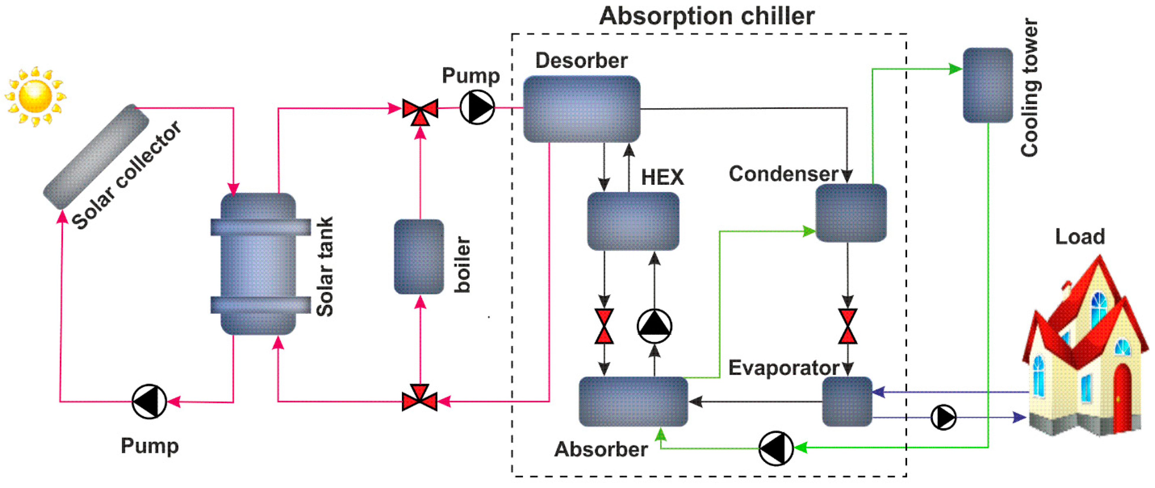
Solar cooling technology uses the solar hot water system as an energy resource for the sorption cycle. The solar absorption cooling system (SACS) under investigation contains two main parts (see Figure 1): the heat medium production and cold medium production. The heat medium production includes solar thermal collectors, a solar tank, auxiliary boiler, two pumps, and a distribution cycle. The cold medium production integrates an absorption chiller, a cooling tower, and two circulating pumps connected, respectively, to the absorber and evaporator. The energy harvested from the incident solar radiation heats the water in a field of the evacuated tube collector (ETC). Then, the hot water flows into a solar tank and is subsequently transported to the absorption chiller through the auxiliary boiler to produce chilled water, which circulates through a conventional distribution system of individual fan coils to deliver cold air to the building. An auxiliary heater is activated if the hot water temperature is not sufficient to drive the chiller. The cooling water dissipates the heat of the absorber and condenser of the chiller through the cooling tower. Figure 1 shows all of the elements that will be taken into account in the simulation and is described, in detail, in the following subsections.
2.1.1. Solar Collector
The evacuated tube collector (ETC) is the most popular solar collector in the world and excels in cloudy and cold conditions. The Apricus ETC-30 solar collector has been selected in this study [29]. The ETC is made up of two concentric glass tubes; the interior acts as a collector and the exterior as a cover. The elimination of air between the tubes reduces energy loss. An advantage of flat absorber vacuum tubes, from architectural integration, is that they can be installed on a horizontal or vertical surface, and the tubes can be rotated so that the absorber is at the appropriate inclination [30]. The collector thermal efficiency is given in Equation (1):
where: is the optical efficiency, and present, respectively, loss coefficient, refers to the difference between the average water temperature through solar collector Tm and the ambient temperature Ta and is the total radiation incident on the absorber surface, for modeling the evacuated tube collectors (ETCs) in TRNSYS, needs an external file of incidence angle modifier (IAM) both longitudinal and transversal, which can be gained from manufacturer catalog. The performance specifications of the ETC are listed in Table 1 [29].
2.1.2. Solar Tank
The capacity of the hot storage tank is a decisive step in the solar system design and depends on the type of installation of three factors: the installed area of collectors, the operating temperature, and the time difference between the capture and storage. In installations for solar cooling, some authors have used values of 25 to 100 L/m2 of the collector area [21]. For the calculation of the solar tank, we will assume that the hot water is stratified. The stratified storage tank comprises N nodes, the i node energy balance is given in Equation (2) [31]:
where: Mi is the fluid mass at the node i, CP is the fluid specific heat, is the mass flow rate from the heat source side, is the mass flow rate of the load side, U is the overall losses from the solar tank to the environment, Ai is the surface transfer area, Ti is the node temperature, and Ta is the ambient temperature. An overall heat transfer coefficient for heat loss between the storage tank and the environment of 1.5 kJ/(h·m2·K) will be assumed, close to that used by Barghouti et al. [31].
2.1.3. Auxiliary Boiler
To operate the absorption chiller when the captured radiation is insufficient and the solar tank is depleted, an auxiliary system is employed to maintain the thermal energy at the desired level to drive the thermal chiller, the thermal energy supplied by the auxiliary boiler can be calculated by Equation (3):
where: Tin is the fluid inlet temperature, Tset is the thermostat set temperature, UAaux refers to the overall coefficient of loss to the environment, is the auxiliary heater efficiency, and Taux is the average temperature can be calculated by Equation (4):
In this work, a boiler with a nominal power of 60 kW (Qe/COP = 35/0.70 = 50 KW) has been selected, and a performance of 90%, which will be assumed constant. For the auxiliary boiler, the parallel arrangement is preferred to prevent its operation from contributing to the heating of the water in the storage tank.
2.1.4. Heat Rejection System: Cooling Tower
A heat rejection system is attached to the thermal absorption chiller in order to evacuate the heat from the absorber and the condenser of the chiller and eject it to the ambient air. In this paper, the counterflow mechanical wet cooling tower was selected with the Baltimore Aircoil Company (BAC, Madrid, Spain) [32], The selected tower is the FXT-26 model, which has the nominal operating conditions listed in Table 2 and it is capable of dissipating all the heat evacuated by the absorption chiller under any environmental conditions in the location of installation (in our case, Baghdad, Iraq). The counterflow, the forced draft-cooling tower can be modeled in TRNSYS, based on the number of transfer units (NTU) [33]:
where: and are the mass flow rates of water and air, respectively, c and n are the coefficients of mass transfer constant and exponent; their values are given by the manufacturer’s curves in this paper, the selected values of c and n are 0.5 and −0.856 respectively.
2.1.5. Cooling Cycle: Absorption
The proposed chiller simulated here is the single-effect LiBr–H2O absorption chiller YAZAKI WFC-SC10 (Yazaki Energy Systems Inc., Plano, TX, USA) with a nominal coefficient of performance (COP) of 0.70 and nominal cooling capacity of 35 kW. The technical specifications of the chiller are listed in Table 3 [34]. For the analysis of facilities, we will always assume a maximum demand capable of being satisfied by this chiller to cover the cooling load (in our case the maximum demand will be 25 kW). The simulation program required data from the chiller catalog that describes the chiller’s operating map in order to determine the operating variables. The absorption machines are usually characterized by two basic parameters:
- →
- COP nominal. COPnom. (0.7 for Yazaki WFC-10, Yazaki Energy Systems Inc., Plano, TX, USA)
- →
- Nominal evaporator power . (35 kW for Yazaki WFC-10, Yazaki Energy Systems Inc., Plano, TX, USA)
From these, the nominal generator power is immediately available by simply dividing the nominal cooling power by the nominal coefficient of performance COPnom. The TRNSYS model also requires entering the target temperature to be obtained at the outlet of the evaporator Te,set, as well as the temperatures and flows entering the three external circuits: evaporator Tei, condenser Tci and generator Tgi. In this way, the model can determine the load regime in which the chiller works. Under these conditions, two situations can occur: if there is sufficient output power available on the evaporator, the set temperature will be reached. If not, the lowest possible value will be reached with the available power.
The instant heat that should be removed from the incoming flow of the child as well as the load fraction fLoad are determined by Equations (6) and (7).
With the load fraction and the temperatures indicated above (set, evaporator, condenser, and generator) it is possible to access the configuration file, whose structure will be commented on later, and which has been made from the chiller operation curves offered by the manufacturer for a set of operation points, establishing two basic parameters:
- →
- Fraction capacity fcapacity: is the ratio of the evaporator’s output power to the nominal power of the chiller. With the manufacturer’s data for each of the established operating points, the quotient between the output power it has in each of these conditions and the nominal power of the evaporator is evaluated.where is the output power under the particular conditions;
- →
- Energy input fraction fEnergyinput: is the ratio of the generator power to the nominal generator power necessary to satisfy the evaporator power. Similarly, it is obtained from the operation curves as:where and COP are the values for the particular evaluation conditions obtained from the manufacture’s curves. The maximum output power that the chiller will be able to offer on the evaporator for each of the conditions evaluated is calculated from Equation (10).
On the other hand, the output power of the evaporator will be the minimum between the maximum power it is capable of offering in each of the conditions, and the demand is given by Equation (11).
With this evaporator power value, the flow rate, and the inlet temperature, the outlet temperature of the evaporator Teo can be determined. Logically, at partial loads.
The generator demand is taken from the energy input fraction fEnergyinput (whose value has been given by the operating curve file for the operating conditions), multiplied by the standardized generator power.
The output temperature is an immediate value, the input temperature, and the generator flow rate are known as shown in Equation (14):
If it is assumed that the machine is adiabatic and, therefore, has no heat loss or gain; the power in the condenser is equal to the sum of the generator plus the evaporator:
The output temperature of the condenser Tco is calculated in the same way as for the evaporator and the generator:
Finally, The COP of the chiller is determined by Equation (17) [35]:
2.2. Meteorological Data
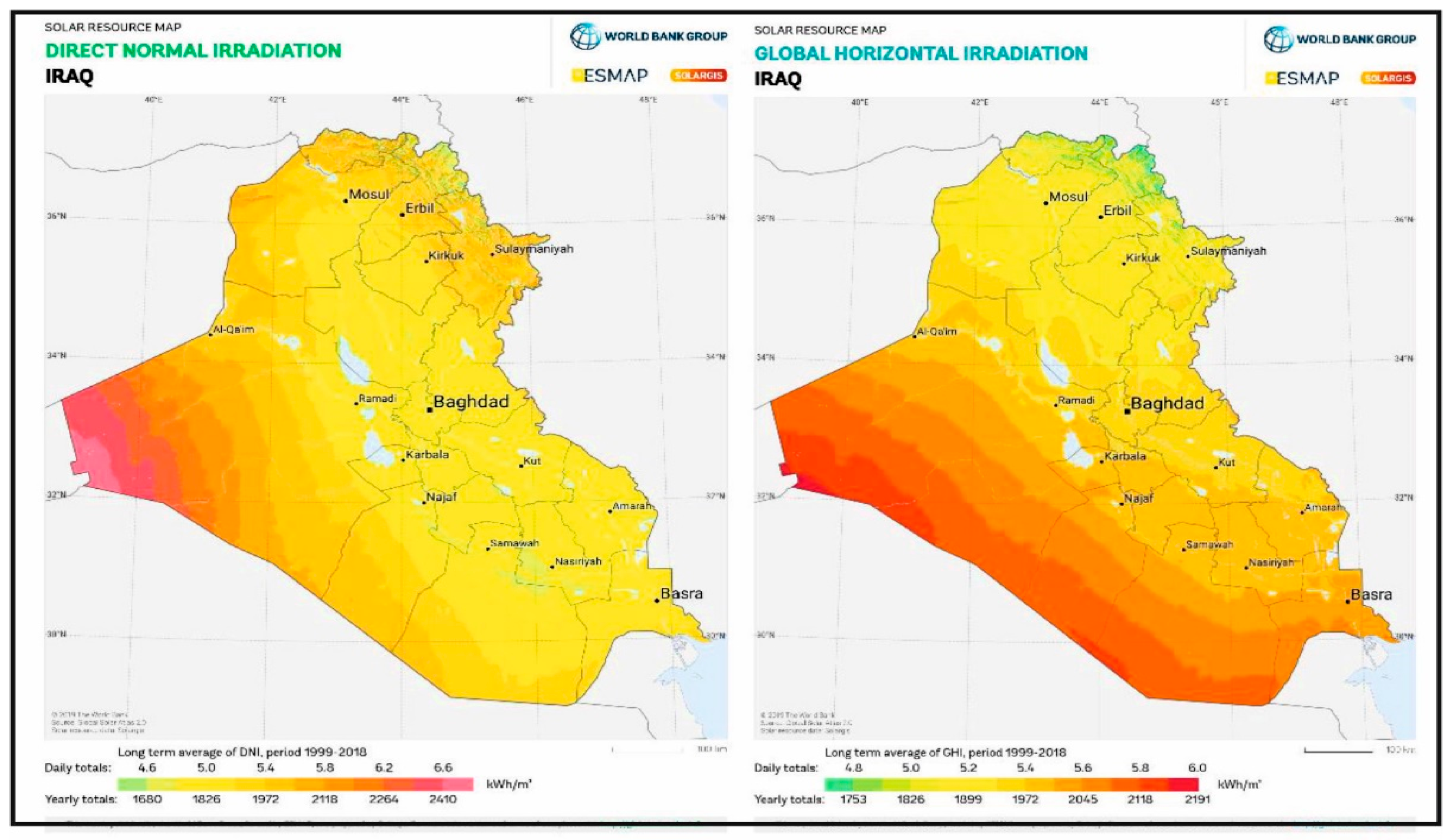
This section will highlight the analysis of potential solar data in Baghdad, Iraq. The main reason for this is to discover the potential power of renewable energy available at the location of operation. The meteorological conditions of Iraq correspond to a warm and dry climate during the summer season. Iraq has abundant solar energy capability with a significant amount of sunlight throughout the year as it is located in the Global Sunbelt. Solar energy can be widely deployed throughout two-thirds of Iraq. In the western and southern areas, daily average radiation ranges between 2800 and 3000 h, with relatively high average daily solar radiation of 6.5–7 kWh/m2. The direct and global solar irradiation is given in Figure 2, [26]. Thence, the study location has great potential for solar energy, allowing sufficient use of solar thermal power as a main prime mover for the absorption cooling system.
The solar radiation data and environmental conditions used correspond to the TMY2 (typical meteorological year) format for Baghdad, the capital of Iraq (latitude is 33.3 N, longitude is 44.6 E, and Altitude 3.8 m). These data are provided by TRNSYS and have been obtained with Version 5 of the Meteonorm program.
Solar insolation varies according to the time of year. The daily highest solar irradiation of the globe is almost 8 kWh/m2 and the daily highest temperature reaches over 45 °C (sometimes in summer season, the temperatures exceed 50 °C). A cooling effect is needed for seven months (April–October). During these months, the sunshine lasts for almost 10 hours per day, with an average total daylight of 13 hours per day [36].
2.3. House Profile and Cooling Loads
The proposed methodology was applied to a residential house located in Baghdad, Iraq. The house layout, wall layer details, and various construction components are given in Appendix A. As for the design of the house: the windows are on the north, east, and west walls; overhangs have a projection factor (overhang depth/window height) of 0.6. Two doors are on the north and east sides. Windows and doors are not specified on the south wall (to minimize heat gain through radiation). The window-to-gross-wall area is kept at 29%. The zone temperature is specified as 25 °C; the new design envelope specifications are as follows:
- The window-to-gross-wall area should not be greater than 35%.
- Overhangs should be placed on the east, west, and south windows of the building with a projection factor (overhang depth/window height) of greater than 0.5.
- Lighting devices should have an efficiency of 60 lumens/W.
- Specific lighting, 15 W/m2.
- Specific gain (equipment and people), 15 W/m2.
- Occupation rate 0.05 occupants/m2.
Concerning the house under study, the monthly cooling demand of the house is variable during the summer season. An enormous portion of that variable is involved in the cooling load configuration due to the (transient) storage nature inherent in the cooling load. The sum of the components of the cooling load gives the total load of the house building. The calculation of the cooling demand was carried out using CARRIER software, version 4.04 (Carrier Software Systems, Syracuse, NY, USA, 2015), based on weather data for Baghdad. The inside conditions: temperature 25 °C and relative humidity 50%, ambient summer design dry-bulb temperature 48 °C, coincident wet-bulb 26 °C and 18.9 °C (daily range). Solar insolation varies according to the time of year, especially from April to October. The house’s peak load occurs in August at 4 p.m., where the maximum outside temperature is about 49 °C. This value should be adopted for design purposes. Figure 3 illustrates the design temperature profiles for August; the maximum total cooling load according to CARRIER software is 25 kW was in August. Figure 4 shows the percentage of the various peak cooling load components.
2.4. System Modeling
The TRNSYS library includes modules (TYPES) that represent the equipment commonly used in energy systems, modules for processing meteorological data, and modules for processing simulation results. The modular structure of TRNSYS gives great flexibility to analyze different types of energy systems. The representation of SACS in TRNSYS, described in the previous section, is illustrated in Figure 5. Table 4 provides information about the most important components of the system, the type of module that represents them, and provides some parameters of the basic design. Figure 5 and Table 4 do not include other components and flows of less importance. The period of simulation in TRNSYS was seven months (cooling season) from 1April 1 (2160 h) until the end of October (7296 h), with a step time simulation of one minute. Baghdad meteorological data was gained from TMY2.
Some of the simplifying assumptions used in the calculation are indicated below:
- The electrical energy consumed by the pumps is neglected.
- Pumps are not supposed to transmit thermal energy to the fluid.
- When the pumps are running the mass, flows remain constant.
- The limit capacity of the chiller is assumed to correspond to a cooling water temperature of 27 °C.
3. Performance Analysis
3.1. Solar Fraction
The SACS performance can be evaluated using solar fraction (solar coverage). This factor demonstrates the solar energy contribution in chilled water production [37]; the following equation enables the calculation of the solar fraction.
where solar gained energy and is energy from the auxiliary heater. can be calculated by:
where is useful collectors’ energy and is the system losses energy.
3.2. Primary Energy Saving
The primary energy (PE) savings is the saved primary energy, electric, and fossil. These values are mathematically described below, in order to evaluate the primary energy consumption of a solar system and a conventional one:
where:
- is the efficiency of auxiliary boiler 0.9;
- is required heat for both space heating and DHW (Domestic Hot Water) in the conventional system (kWh).
- is the produced energy by auxiliary heater (kWh).
- , are the primary energy conversion factors for heat and electricity from fossil fuel, 0.95 kWhheat,fossil/kWhPE and 0.5 kWhelec,fossil/kWhPE.
3.3. Electric Efficiency of the Total System
The electric efficiency is the relationship of the total heating and cooling energy generation to the required electricity for this production. The total system electrical efficiency is given by:
where:
- is the consumed electricity by a pump that feeds the chiller (kWh).
- is the consumed electricity by cooling water loop pump (kWh).
- is the consumed electricity by the chiller (kWh).
- is the electrical power of fan cooling tower (kWh).
- is the consumed electricity by solar loops pumps (kWh).
- is the consumed electricity by boiler (kWh).
4. Results and Discussion
4.1. House Energy Balance Analysis
In this section, the thermal energy balance of SACS for the house under study was established through the evaluation of harvested solar energy, the delivered energy from a hot solar tank, the energy from the auxiliary boiler, and the necessary energy to satisfy the load. Table 5 shows the important and vital information efficiency parameters (result of SACS) for the summer season.
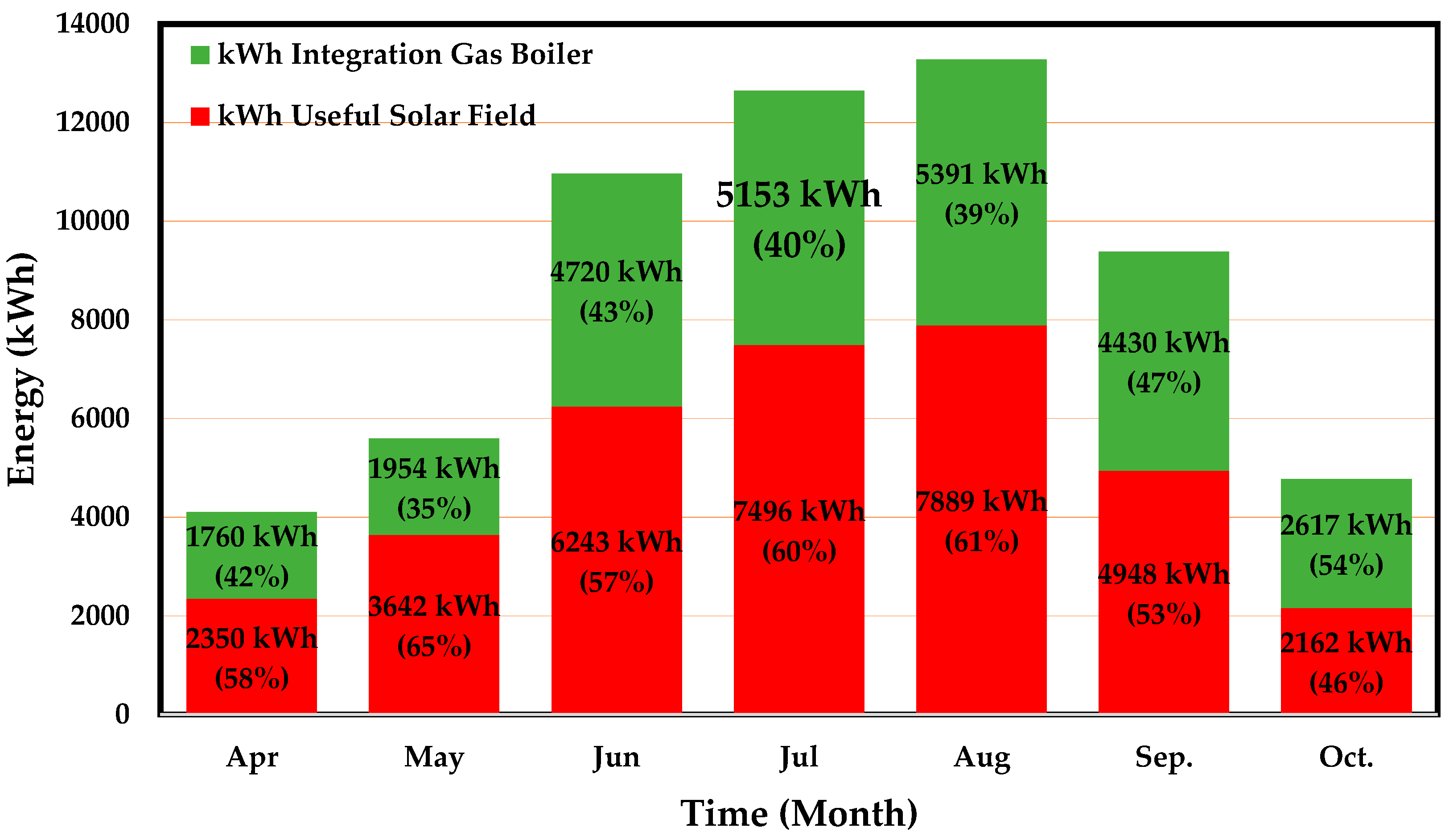
Figure 6 and Figure 7 show, respectively, the energy contribution of the integrated gas boiler and solar field during the cooling season. The analyses results show that the useful energy of the solar field was 34,730 kWh and the energy delivered by the boiler was 26,025 kWh, indicating that the total season solar fraction (also called solar coverage) to the load was about 58% (see Figure 7). It is clearly seen that the system operating in May had the highest average solar fraction (a value of about 65%) due to the higher value of captured energy and the lower cooling load. Contrarily, the system presenting the lowest average value of solar fraction (45%) operated under October weather conditions. This is because of the lower energy supplied by the storage tank and lower harvested energy by ETC collectors (see Table 5). This outcome reflects the effect of solar irradiation on the energy performance of SACS.
It is also clear that there is a significant impact on the solar fraction from the weather data each month, particularly, solar irradiation that has a direct influence on the energy generated by the ETC field. It is possible to observe this by referring to Equation (18).
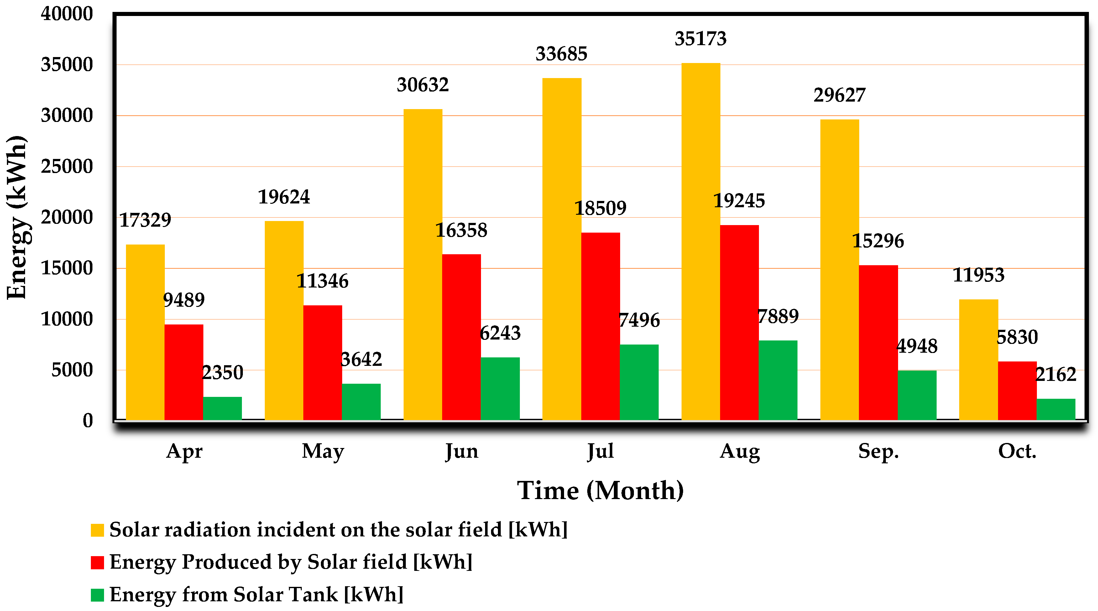
Figure 8 shows the energy contribution of solar irradiation, energy from solar collectors, and solar tank. The average monthly values of incident solar radiation energy on the solar collectors was 178,023 kWh, while the total captured solar energy was 96,073 kWh, and the energy from the solar tank was 34,730 kWh, which implies that the efficiency of ETC collectors during the cooling season was about 54% (see Table 5).
Table 5 outlines the evaluation of the COP over six months, indicating that the average COP of SACS ranges between 0.39 and 0.52. It was also found that the system, operating in July and August, has the best average COP (a value of 0.51 and 0.52), respectively, due to a large amount of captured energy by ETC and a large cooling load that is led to higher solar coverage. Moreover, the lowest average COP (0.39) was recorded in April. Based on Equation (17), we can conclude that the variation in COP (see Table 5) through the six months is directly reported to the thermal energy at the input and output of the generator, and evaporator of the absorption chiller. The COP strongly depends on the flows of energy in these two parts. In general, the generator is influenced by the solar radiation of each month, while the evaporator is affected by building a cooling load, which depends on the ambient outdoor temperature of each month.
4.2. Primary Energy Analysis
The target of this analysis is to find the configuration that optimizes the system performance. Sensitivity analysis is presented under a different number of collectors (areas) and solar tank sizing. The number of collectors, and storage size, in the base case is 12 (30 m2) and 50 L/m2 (1500 L), respectively, compared with the base case. The sensitivity analysis includes changing the surface collector area from 25 m2 to 35 m2; the solar tank volume varied from 1000 l to 2000 l. The results are displayed in Table 6.
It is shown that, with a greater collector area, the best results were obtained. A 16.6% increase in collector surface area is followed by an increase in the solar fraction and relative PE saved, 12.6% and 48.3%, respectively. Regarding solar tank volume, it is clearly seen that variation of tank volume does not present a significant influence on solar fraction, electrical efficiency, and PE relative; a solar tank volume increasing of 33.3% reflects on increasing in a solar fraction of about 2.5%, and PE relative around 10.3%. From the previous results, it can be recommended to use a collector area of 35 m2 and a storage tank volume of 2000 L in order to achieve better performance than that reached in the base case.
4.3. Parametric Analysis
In this section, a parametric analysis has been carried out, taking into consideration the main important design parameters: the collector slope, water flow rate through the collector, number of collectors, and the solar tank size. In all analyses carried out below, the value of a single parameter is modified keeping the rest in the value corresponding to the base design.
4.3.1. Effect of Collector Slope
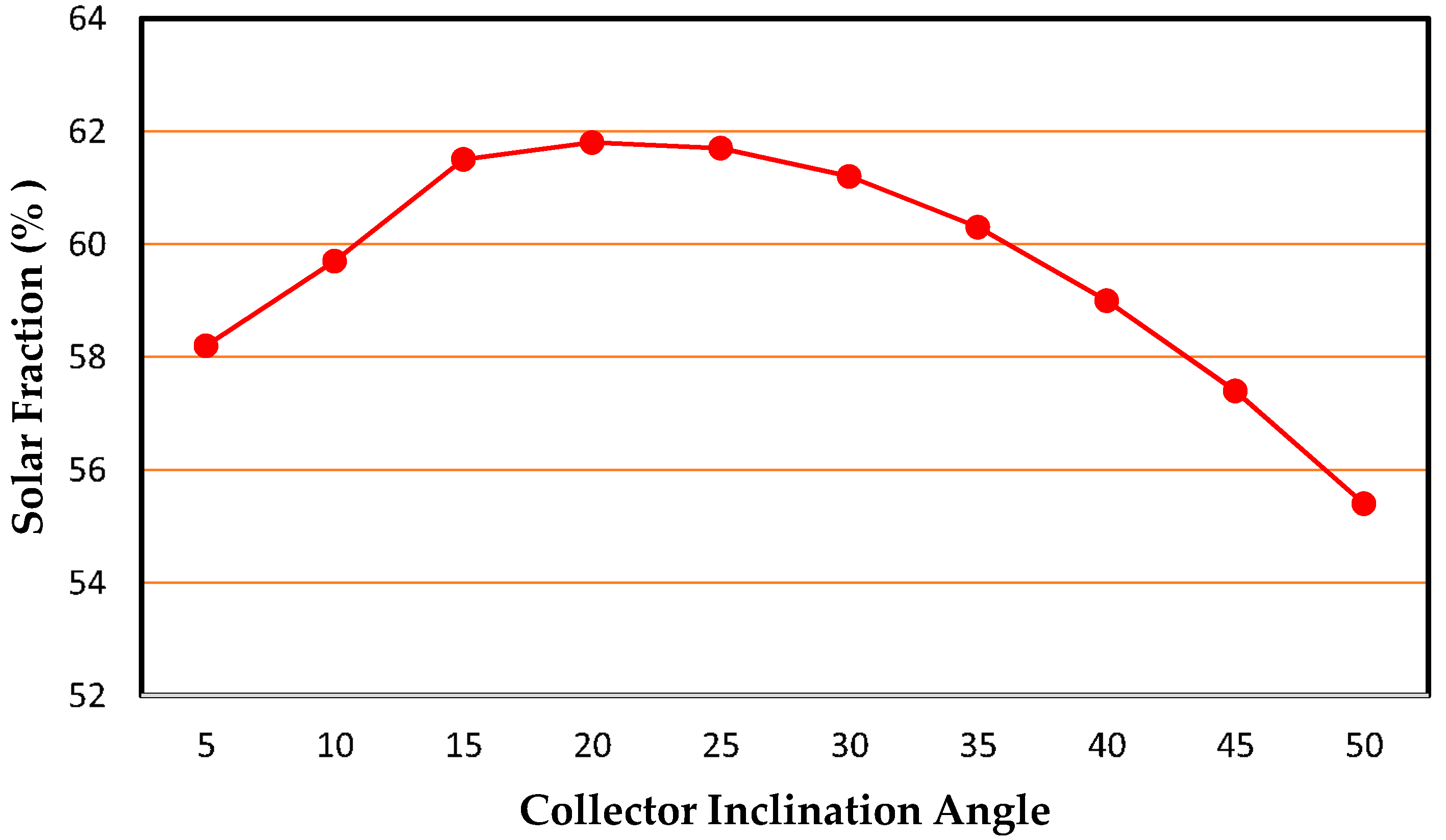
The inclination angle of the collector has a significant impact on the overall SACS performance. Figure 9 shows the variation in solar coverage with the collector field inclination in Baghdad. The evaluation based on a change in the tilt angle from 5° to 50° by a step of 5° was carried out in order to compute the optimum angle of the solar field that provides the highest solar fraction. The change in this variable shows that the tilt angles (15°, 20°, 25°, 30°) give a higher solar fraction, contrarily to the last three angles where solar fraction decreases. The reason for this difference is solar radiation perpendicularity that provides optimal results during summer with low tilt angle values, which help capture more solar radiation, as reported by Shariah and Elminir [38,39]. The optimum tilt values giving higher solar fraction are between 15° and 25°; therefore, operating at optimum value for tilt angles can readily expand the amount of solar energy incident and, thus, enhance both the thermal and economic efficiency of the SACS.
4.3.2. Effect of Water Flow Rate
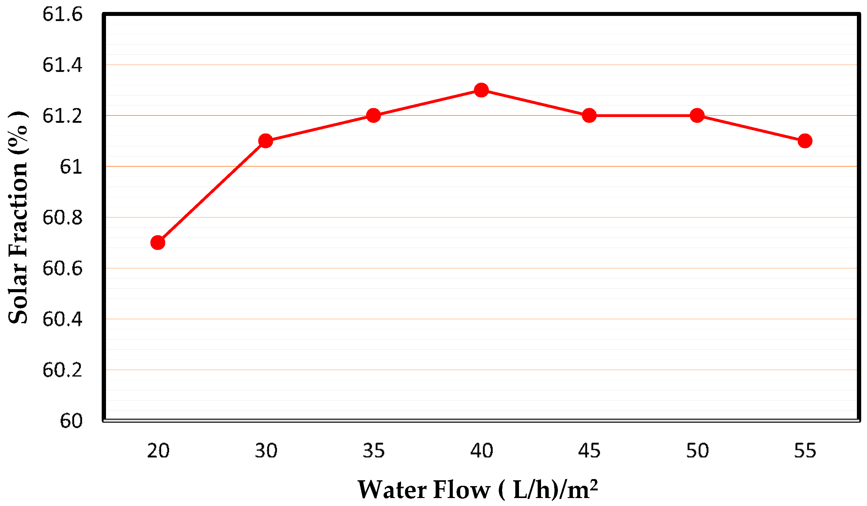
In the literature, the hot water flow rate values through solar collectors range from 20 to 80 L/h per m2 of collector area are recommended for panels connected in parallel, as in our case. The variation of the solar fraction, with the hot water flow rate through the solar collector array, is indicated in Figure 10. The water flow rate varied from 20 to 55 (L/h)/m2 of collector area. A change of water flow from 20 to 40 (L/h)/m2 causes only a 0.9% increase in solar fraction; increasing the flow rate over an optimum value (40 (L/h)/m2) will lead to drops in a solar fraction of about 0.2%. It is evident that the results obtained depict small changes in solar fraction and allow us to affirm that this parameter does not present a significant impact on solar coverage; it is in alignment with the results obtained by Beckman [40,41].
4.3.3. Effect of Solar Field Area
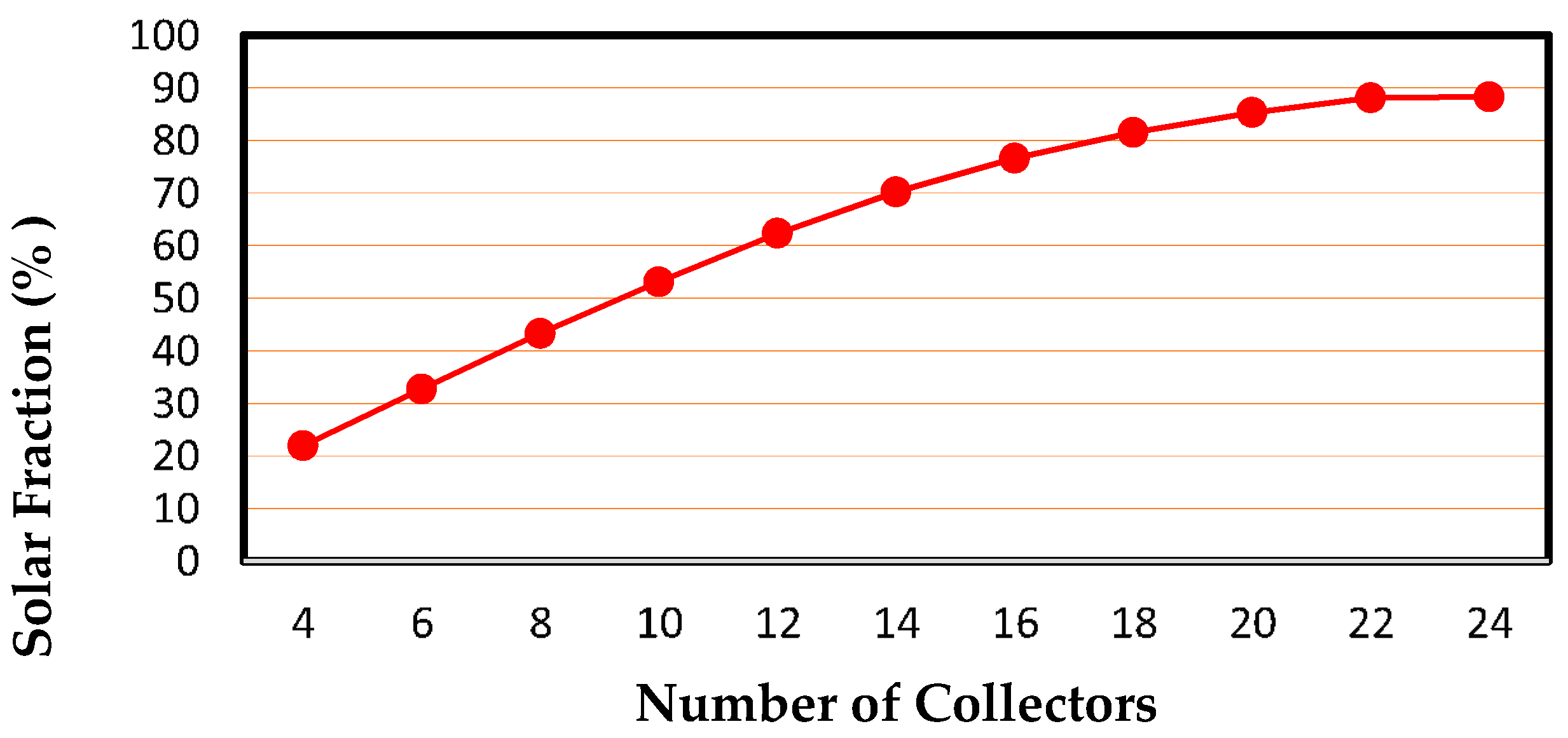
The area and the number of solar collectors play an important role in determining the optimal configuration of the capture solar system. The collector surface has a decisive effect on the efficiency and feasibility of SACS. The simulation was carried out to establish the influence of this parameter on the overall performance of SACS under study, based on the collector’s tilt angle 20°. The area of each collector was 2.5 m2, the water flow rate was 40 L/h per m2, the solar tank volume was 30 L/m2; the lower and upper solar tank temperatures were Tlower = 75 °C, Tupper = 90 °C. Figure 11 depicts the variation of the solar fraction with the number of collectors installed. The evaluation involves changing the number of a collectors from 4 to 24 (10 m2 to 60 m2) by a step of 2 (2 m2). It is clear that an increase in the collector surface area tends to enhance solar coverage due to the proportion between the captured energy from the ETC field and solar fraction, according to simulation results displayed in Figure 11. It is predicted that the solar coverage stays constant, especially at the higher solar surface field (˃55 m2). As an example, an evacuated tube collector operating in Baghdad, inclination angle 30 degrees, presents a solar coverage of about 88.1% for 22 collectors (55 m2) and 88.3% for 24 collectors (60 m2). The stability in solar fraction SF (Solar Fraction), which was also achieved in published works Bahria and Assilzadeh [42,43], indicates that the system achieves its optimum level, and any additional increase in the surface field leads to overproduction of thermal energy, which can cause technological problems and significantly increase the initial investment. Therefore, with equal investment costs, the best design will be the one that offers the greatest coverage.
4.3.4. Effect of Solar Tank Capacity
This section examines the influence of the solar tank capacity on the solar fraction. The literature recommends values of storage solar tank capacity from 20 to 100 L/m2 of collector area for installations where the time delay between collection and consumption does not exceed 24 h. The solar fraction is not significantly affected by the change in storage tank capacity, as shown in Figure 12. It is clear that increasing the solar tank capacity has a slight effect on the solar fraction. A change in solar accumulator capacity from 10 to 55 L/m2 of the collector area obtains an increase in solar coverage of only 60.6% to 61.1%, respectively, with this difference (0.5%) observed—that the effect of the solar tank size on solar coverage is not significantly high. The optimum capacity of the solar tank, 30 L/m2, gives solar coverage of 61.6%. Figure 12 depicts that the oversized solar tank will cause a decrease in solar fraction due to increases in thermal losses. The result in Figure 12 is in alignment with that of Beckman [40,41]. Therefore, it is not surprising that the optimal accumulator capacity is at the lower values of the recommended range.
4.3.5. Effect of Solar Tank Temperature
Table 7 and Table 8 present the results obtained for the variation of the solar fraction with the lower and upper temperatures of the solar tank that defines the operating of the absorption chiller with solar heat. The absorption chiller will operate with water from the solar accumulator tank when the upper temperature of the storage tank is between these limits and it is possible to completely cover the cold demand. Concerning the upper temperature, the value of 90 °C used in the basic design seems reasonable; a higher value of top solar tank temperature would improve the solar coverage somewhat, but it should be taken into account that the limit of 95 °C, imposed by the absorption chiller, cannot be exceeded. In fact, tank temperature affects, as well, the inlet temperature of the generator, since the hot water directly supplies the chiller generator. As for the lower temperature, the advantage of using values as small as possible is clear. This is because more solar heat can be used and the efficiency of the collector can be improved.
5. Conclusions
This article presented a detailed analysis of the performance of a solar driven-absorption cooling system as alternative technology for air conditioning of a house, under hot and dry climate in Baghdad, Iraq. Various parameters influencing the solar fraction and the solar cooling performance of the proposed system have been discussed.
Based on the results of the simulation performed in this work, it was revealed that weather conditions have a significant effect on the performance of the solar absorption air conditioning system, with peak loads during the summer months. August presented the highest performance. The relevant average COP achieved a value of 0.52 while the solar fraction was 59.4%.
The results (of energy analysis contribution) during the summer season showed that the amount of energy incident was 178,023 kWh, while the total energy harvested was 96,073 kWh, which implies that the efficiency of ETC collectors during the cooling season is about 54%. It was also found that the solar energy supplied by the solar tank was 34,730 kWh and the energy delivered by the boiler was 26,025 kWh, indicating that the total seasonal solar coverage was about 58%.
The results of the primary energy analysis evidenced the use of a collector area of 35 m2; a storage tank volume of 2000 L presented better performance than that reached in the base case.
Parametric analysis results showed the best configuration for the design of SACS. It was found that the solar collector tilt angle is significantly affected by the incident solar irradiation. An optimal value (between 15° and 25°) of the inclination presented a higher solar fraction. It was also found that increasing the water flow rate through the collectors does not indicate a significant effect on solar coverage.
The surface collector analysis revealed that, in general, the increase of the installed surface of the collector field leads to improve the solar fraction values. It was also found that the solar fraction remained the same for an area larger than 55 m2. Therefore, it is concluded that the appropriate collector surface selection should be carried out together with economic and technical feasibility (mainly cost analysis and land availability) in order to achieve the best profitability of the system.
Moreover, the change in the size of the solar tank has no significant impact on the solar fraction (60.6% and 61.1% for 10 L/m2 and 55 L/m2 of collector area, respectively). Increasing the upper solar tank temperature improves the solar coverage, but it should be <95 °C.
Finally, this work provides a roadmap for designers, in particular, to ensure that all of the operating and design variable effects are taken into consideration when developing a solar air-conditioning cycle under the Iraq climate. Additionally, the model can be employed to carry out thermo-economic comparisons of the system using various types of collectors.
Author Contributions
Conceptualization, A.A.-F.; methodology, A.A.-F.; validation, A.A.-F.; formal analysis, A.A.-F.; investigation, A.A.-F.; data curation, A.A.-F.; writing—original draft preparation, A.A.-F.; writing—review and editing, F.A.; supervision, B.E. All authors have read and agreed to the published version of the manuscript.
Funding
The authors received no specific funding for this work. The corresponding author would like to thank the Technical University of Darmstadt, enabling the open-access publication of this paper.
Conflicts of Interest
The authors declare no conflict of interest.
Nomenclatures, Subscripts and Abbreviations
| Nomenclatures | |
| area (m2) | |
| loss coefficient | |
| efficiency | |
| radiation incident (W/m2) | |
| mass flow rate (kg/s) | |
| specific heat (kPa) | |
| heat transfer rate (kW) | |
| temperature (°C) | |
| overall heat transfer coefficient (kW/m2·K) | |
| power (kW) | |
| Subscripts | |
| a | Ambient |
| Auxiliary | |
| Condense | |
| Evaporator | |
| Fraction | |
| Generator | |
| i | Node |
| Load | |
| Nominal | |
| Minimum | |
| Maximum | |
| Outlet | |
| Source | |
| Set | |
| Water | |
| Abbreviations | |
| COP | Coefficient of performance |
| DHW | Domestic hot water |
| EES | Engineering Equation Solver |
| ETC | Evacuated tube collector |
| HVAC | Heating, ventilation, and air conditioning |
| IEA | International Energy Agency |
| IAM | Incidence angle modifier |
| NTU | Number of transfer unit |
| PE | Primary energy |
| SACS | Solar absorption cooling system |
| SF | Solar fraction |
| TMY | Typical meteorological year |
| TRNSYS | Transient System Simulation Program |
Appendix A
The House under Study
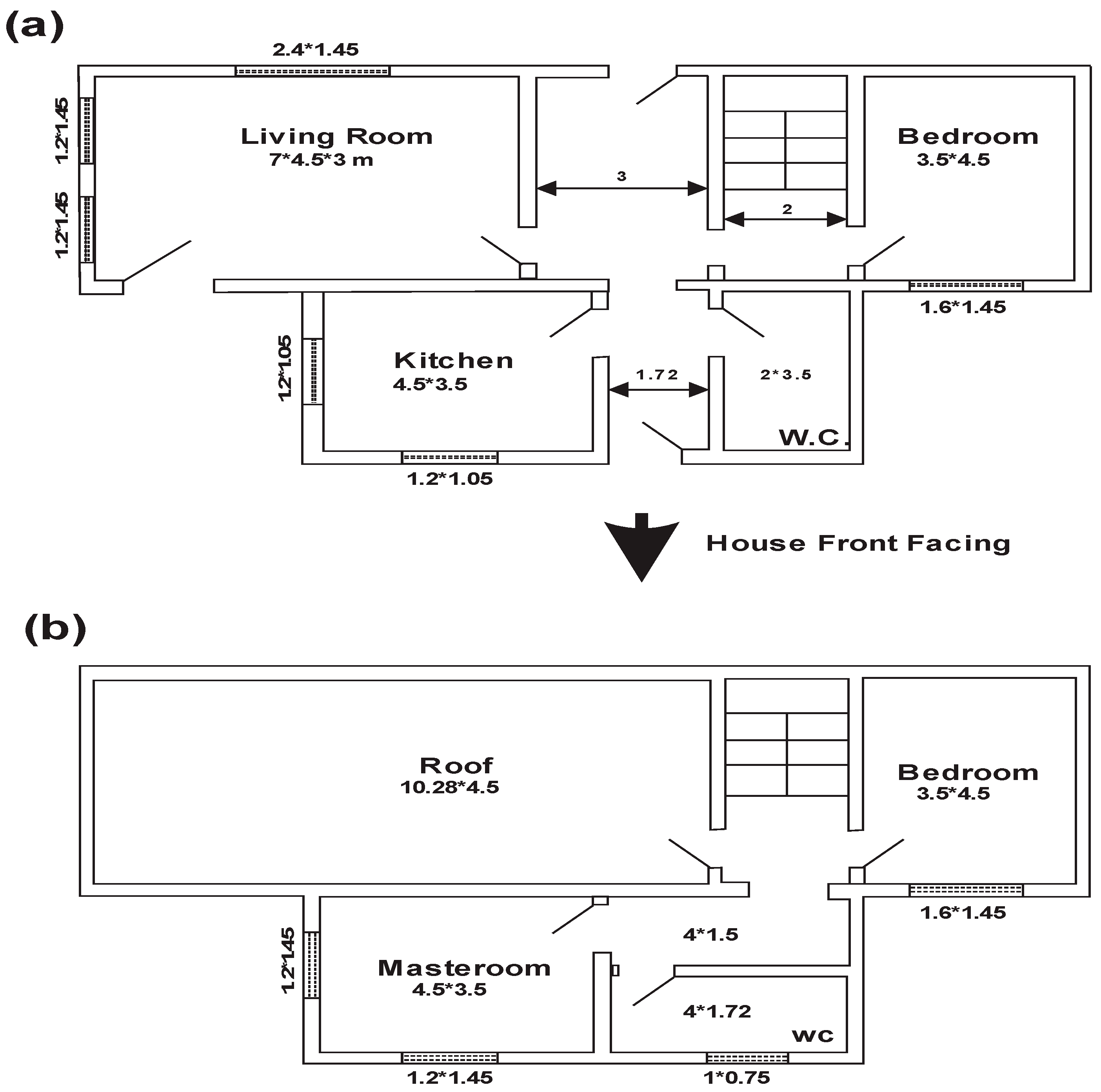
The house building is double dwelling, connected by internal stairs, as shown in Figure A1 [37]. Each floor has an area of 97 m2 and a height of 3 m. The ground floor includes an entrance, living room, bedroom, kitchen, and bathroom. The first floor contains the master room, bedrooms, and bathroom. The wall layer details and various construction components of the house are given in Table A1 and Table A2.
The maximum total calculated cooling load, according to CARRIER software, is about 25 kW. Figure 4 shows the percentage of the various peak cooling load components estimated by CARRIER software. The load through the walls was 40% of the total cooling load due to the higher temperature difference between outdoor and indoor temperature; the heat envelope transmission aggravates cooling demand. The transmission losses could be reduced significantly with envelope higher thickness insulation. Additionally, ETC collectors mounted on the first floor roof of the house could reduce the cooling load due to shading, though not all are eliminated. The load on the roof is 20% of the overall cooling load. The actual total estimated cooling load would be about 21, which is in alignment with the data obtained in [37].
Figure A1.
Layout diagram of the modern domestic solar house (a) ground floor (b) first floor.

Table A1.
Wall layers details.
| Wall Details Outside Surface Color Dark Absorptivity 0.900 Overall U-Value 0.415 W/(m2·K) | |||||
|---|---|---|---|---|---|
| Wall Layers Details (Inside to Outside) | |||||
| Layers | Thickness mm | Density kg/m3 | Specific Ht·kJ/(kg·K) | R-Value (m2·K)/W | Weight kg/m2 |
| Inside surface resistance | 0.000 | 0.0 | 0.00 | 0.00200 | 0.0 |
| Cement bounded | 12.000 | 1600.0 | 1.34 | 0.04200 | 19.2 |
| Insulation | 50.000 | 32.0 | 0.90 | 1.66600 | 1.6 |
| Hollow block | 200.000 | 1922.0 | 0.84 | 0.40000 | 384.4 |
| 13 mm gypsum board | 12.700 | 800.9 | 1.09 | 0.07890 | 10.2 |
| Outside surface resistance | 0.000 | 0.0 | 0.00 | 0.00200 | 0.0 |
| Air space | 0.000 | 0.0 | 0.00 | 0.16026 | 0.0 |
| Outside surface resistance | 0.000 | 0.0 | 0.00 | 0.05864 | 0.0 |
| Totals | 274.700 | - | - | 2.40980 | 415.4 |
Table A2.
Construction components of the house.
| Component | Exterior Roof | Exterior Glass | Exterior Wooden Door | Exterior Steel Door |
|---|---|---|---|---|
| U value (W/m2 °C) | 1.670388 | 5.888993 | 2.087049 | 6.07040 |
References
- Allouhi, A.; El Fouih, Y.; Kousksou, T.; Jamil, A.; Zeraouli, Y.; Mourad, Y. Energy consumption and efficiency in buildings: Current status and future trends. J. Clean. Prod. 2015, 109, 118–130. [Google Scholar] [CrossRef]
- Dahl, R. Cooling concepts: Alternatives to air conditioning for a warm world. Environ. Health Perspect. 2013, 121, a18–a25. [Google Scholar] [CrossRef] [PubMed] [Green Version]
- Rashid, S.; Peters, I.; Wickel, M.; Magazowski, C. Electricity Problem in Iraq. In Economics and Planning of Technical Urban Infrastructure Systems; HafenCity Universität Hamburg: Hamburg, Germany, 2012. [Google Scholar]
- Allouhi, A.; Kousksou, T.; Jamil, A.; El Rhafiki, T.; Mourad, Y.; Zeraouli, Y. Economic and environmental assessment of solar air-conditioning systems in Morocco. Renew. Sustain. Energy Rev. 2015, 50, 770–781. [Google Scholar] [CrossRef]
- Petela, K.; Szlęk, A. Assesment of Passive Cooling in Residential Application under Moderate Climate Conditions. Ecol. Chem. Eng. A 2016, 23, 211–225. [Google Scholar]
- Baniyounes, A.M.; Rasul, M.G.; Khan, M.M.K. Assessment of solar assisted air conditioning in Central Queensland’s subtropical climate, Australia. Renew. Energy 2013, 50, 334–341. [Google Scholar] [CrossRef]
- Balghouthi, M.; Chahbani, M.H.; Guizani, A. Feasibility of solar absorption air conditioning in Tunisia. Build. Environ. 2008, 43, 1459–1470. [Google Scholar] [CrossRef]
- Martínez, P.J.; Martínez, J.C.; Lucas, M. Design and test results of a low-capacity solar cooling system in Alicante (Spain). Sol. Energy 2012, 86, 2950–2960. [Google Scholar] [CrossRef]
- Burckhart, H.J.; Audinet, F.; Gabassi, M.-L.; Martel, C. Application of a novel, vacuum-insulated solar collector for heating and cooling. Energy Procedia 2014, 48, 790–795. [Google Scholar] [CrossRef] [Green Version]
- Ketjoy, N.; Rawipa, Y.; Mansiri, K. Performance evaluation of 35 kW LiBr H2O solar absorption cooling system in Thailand. Energy Procedia 2013, 34, 198–210. [Google Scholar] [CrossRef] [Green Version]
- Leiva-Illanes, R.; Escobar, R.; Cardemil, J.M.; Alarcón-Padilla, D.-C. Comparison of the levelized cost and thermoeconomic methodologies—Cost allocation in a solar polygeneration plant to produce power, desalted water, cooling and process heat. Energy Convers. Manag. 2018, 168, 215–229. [Google Scholar] [CrossRef]
- Jenkins, P.; Elmnifi, M.; Younis, A.; Emhamed, A.; Alshilmany, M. Design of a Solar Absorption Cooling System: Case Study. J. Power Energy Eng. 2020, 8, 1–15. [Google Scholar] [CrossRef] [Green Version]
- Wang, K.; He, Y.; Kan, A.; Yu, W.; Wang, D.; Zhang, L.; Zhu, G.; Xie, H.; She, X. Significant photothermal conversion enhancement of nanofluids induced by Rayleigh-Bénard convection for direct absorption solar collectors. Appl. Energy 2019, 254, 113706. [Google Scholar] [CrossRef]
- Mukhtar, H.K.; Said, S.A.; El-Sharaawi, M.I. Dynamic performance of solar powered vapor absorption cooling system in dhahran—Saudi Arabia. In Proceedings of the 2018 5th International Conference on Renewable Energy: Generation and Applications (ICREGA), Al Ain, United Arab Emirates, 26–28 February 2018. [Google Scholar]
- Elahi, R.; Nagassou, D.; Trelles, J.; Mohsenian, S.; Trelles, J. Enhanced solar absorption by CO2 in thermodynamic noneq. Sol. Energy 2019, 195, 369–381. [Google Scholar] [CrossRef]
- Behi, M.; Mirmohammadi, S.A.; Ghanbarpour, M.; Behi, H.; Palm, B. Evaluation of a novel solar driven sorption cooling/heating system integrated with PCM storage compartment. Energy 2018, 164, 449–464. [Google Scholar] [CrossRef]
- Salehi, S.; Yari, M.; Rosen, M.A. Exergoeconomic comparison of solar-assisted absorption heat pumps, solar heaters and gas boiler systems for district heating in Sarein Town, Iran. Appl. Therm. Eng. 2019, 153, 409–425. [Google Scholar] [CrossRef]
- Buonomano, A.; Calise, F.; Dentice D’accadia, M.; Ferruzzi, G.; Frascogna, S.; Palombo, A.; Russo, R.; Scarpellino, M. Experimental analysis and dynamic simulation of a novel high-temperature solar cooling system. Energy Convers. Manag. 2016, 109, 19–39. [Google Scholar] [CrossRef]
- Mateus, T.; Oliveira, A.C. Energy and economic analysis of an integrated solar absorption cooling and heating system in different building types and climates. Appl. Energy 2009, 86, 949–957. [Google Scholar] [CrossRef]
- Fedrizzi, R.; Franchini, G.; Mugnier, D.; Melograno, P.N.; Theofilidi, M.; Thuer, A.; Nienborg, B.; Koch, L.; Fernandez, R.; Troi, A.; et al. Assessment of Standard Small-Scale Solar Cooling Configurations within the SolarCombi+ Project. In Proceedings of the 3rd International Conference Solar Air-Conditioning, Palermo, Italy, 30 September–2 October 2009. [Google Scholar]
- Shirazi, A.; Taylor, R.A.; White, S.D.; Morrison, G.L. Transient simulation and parametric study of solar-assisted heating and cooling absorption systems: An energetic, economic and environmental (3E) assessment. Renew. Energy 2016, 86, 955–971. [Google Scholar] [CrossRef]
- Vasta, S.; Palomba, V.; Frazzica, A.; Costa, F.; Freni, A. Dynamic simulation and performance analysis of solar cooling systems in Italy. Energy Procedia 2015, 81, 1171–1183. [Google Scholar] [CrossRef] [Green Version]
- Calise, F.; d’Accadia, M.D.; Palombo, A. Transient analysis and energy optimization of solar heating and cooling systems in various configurations. Sol. Energy 2010, 84, 432–449. [Google Scholar] [CrossRef]
- Djelloul, A.; Draoui, B.; Moummi, N. Simulation of a solar driven air conditioning system for a house in dry and hot climate of algeria. Courr. Savoir 2013, 15, 31–39. [Google Scholar]
- Hassan, L.; Moghavvemi, M.; Mohamed, H.A.F. Impact of UPFC-based damping controller on dynamic stability of Iraqi power network. Sci. Res. Essays 2011, 6, 136–145. [Google Scholar]
- The World Bank. Available online: https://solargis.com/maps-and-gis-data/download/iraq (accessed on 5 December 2019).
- Nafey, A.S.; Sharaf, M.A.; García-Rodríguez, L. A new visual library for design and simulation of solar desalination systems (SDS). Desalination 2010, 259, 197–207. [Google Scholar] [CrossRef]
- Sharaf Eldean, M.A.; Soliman, A.M. A new visual library for modeling and simulation of renewable energy desalination systems (REDS). Desalin. Water Treat. 2013, 51, 6905–6920. [Google Scholar] [CrossRef]
- Available online: http://www.apricus.com/en/america/products/solar-collectors/ap-30/ (accessed on 6 December 2019).
- Peuser, F.; Remmers, K.; Schnauss, M. Solar Thermal Systems: Successful Planning and Construction; Routledge: Abingdon, UK, 2013. [Google Scholar]
- Balghouthi, M.; Chahbani, M.H.; Guizani, A. Solar powered air conditioning as a solution to reduce environmental pollution in Tunisia. Desalination 2005, 185, 105–110. [Google Scholar] [CrossRef]
- Available online: http://www.BaltimoreAircoil.com (accessed on 16 December 2019).
- ASHRAE. Heating, Ventilating, and Air-Conditioning Systems and Equipment, SI ed.; American Society of Heating, Refrigerating and Air-Conditioning Engineers, Inc.: Atlanta, GA, USA, 2012. [Google Scholar]
- Available online: http://www.yazakienergy.com (accessed on 31 January 2020).
- Rodríguez-Hidalgo, M.D.C.; Rodríguez-Aumente, P.A.; Lecuona, A.; Legrand, M.; Ventas, R. Domestic hot water consumption vs. solar thermal energy storage: The optimum size of the storage tank. Appl. Energy 2012, 97, 897–906. [Google Scholar]
- Allouhi, A.; Kousksou, T.; Jamil, A.; Bruel, P.; Mourad, Y.; Zeraouli, Y. Solar driven cooling systems: An updated review. Renew. Sustain. Energy Rev. 2015, 44, 159–181. [Google Scholar] [CrossRef]
- Joudi, K.A.; Dhaidan, N.S. Application of solar assisted heating and desiccant cooling systems for a domestic building. Energy Convers. Manag. 2001, 42, 995–1022. [Google Scholar] [CrossRef]
- Shariah, A.; Al-Akhras, M.A.; Al-Omari, I.A. Optimizing the tilt angle of solar collectors. Renew. Energy 2002, 26, 587–598. [Google Scholar] [CrossRef]
- Elminir, H.K.; Ghitas, A.E.; El-Hussainy, F.; Hamid, R.; Beheary, M.M.; Abdel-Moneim, K.M.; Elminir, H.K. Optimum solar flat-plate collector slope: Case study for Helwan, Egypt. Energy Convers. Manag. 2005, 47, 624–637. [Google Scholar] [CrossRef]
- Duffie, J.A.; Beckman, W.A. Solar Engineering of Thermal Processes; John Wiley & Sons: Hoboken, NJ, USA, 1991. [Google Scholar]
- Duffie, J.A.; Beckman, W.A. Solar Engineering of Thermal Processes; John Wiley & Sons: Hoboken, NJ, USA, 2013. [Google Scholar]
- Bahria, S.; Amirat, M.; Hamidat, A.; El Ganaoui, M.; Slimani, M.E.A. Parametric study of solar heating and cooling systems in different climates of Algeria–A comparison between conventional and high-energy-performance buildings. Energy 2016, 113, 521–535. [Google Scholar] [CrossRef]
- Assilzadeh, F.; Kalogirou, S.A.; Ali, Y.; Sopian, K. Simulation and optimization of a LiBr solar absorption cooling system with evacuated tube collectors. Renew. Energy 2005, 30, 1143–1159. [Google Scholar] [CrossRef]
Figure 1.
Solar absorption cooling system components.

Figure 2.
Iraq solar annual direct normal and global horizontal Irradiation map © 2019 The World Bank, Source: Global Solar Atlas 2.0, Solar resource data: Solargis [26].
Figure 2.
Iraq solar annual direct normal and global horizontal Irradiation map © 2019 The World Bank, Source: Global Solar Atlas 2.0, Solar resource data: Solargis [26].

Figure 3.
Design temperature profiles for August.
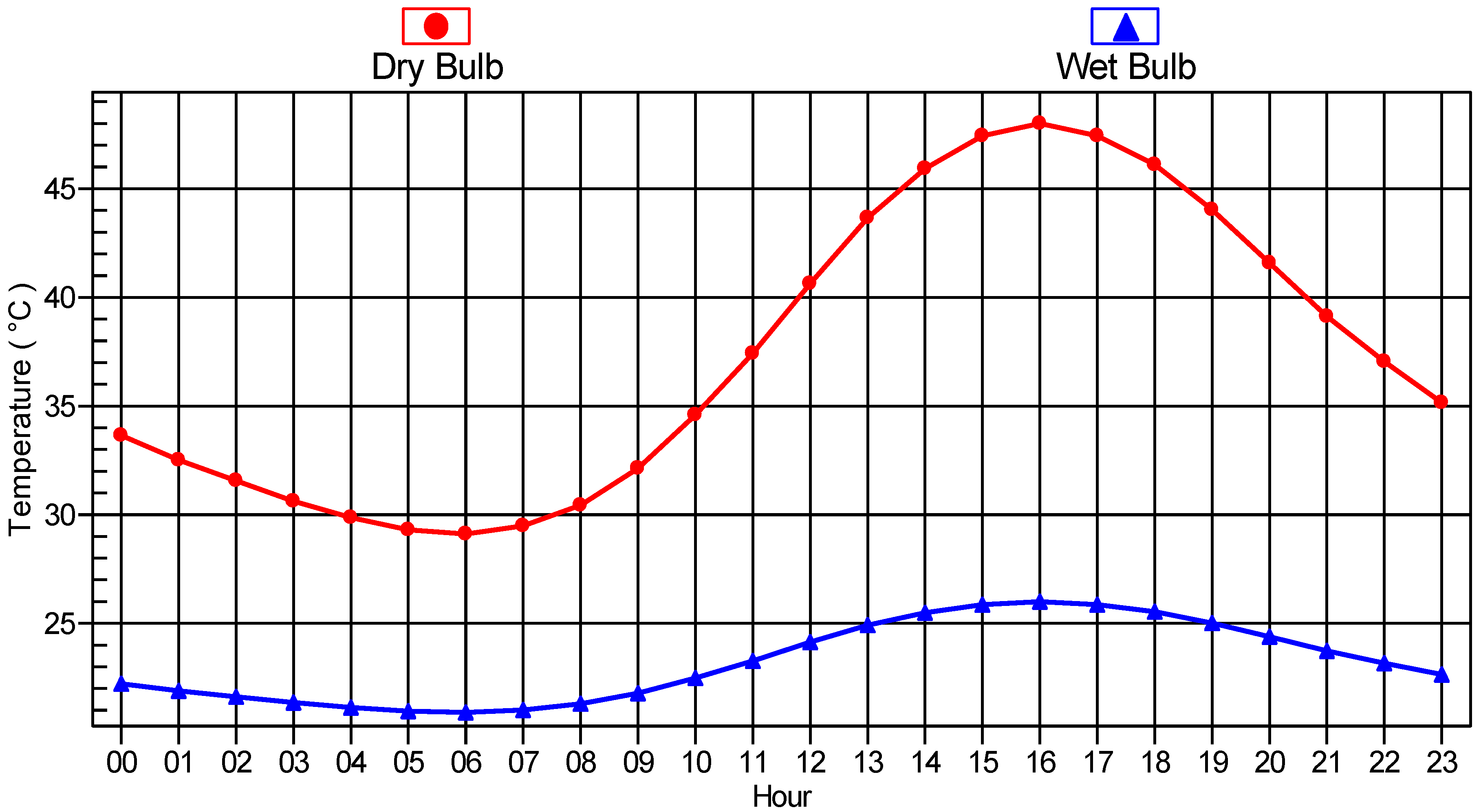
Figure 4.
Contribution of the various cooling load component.
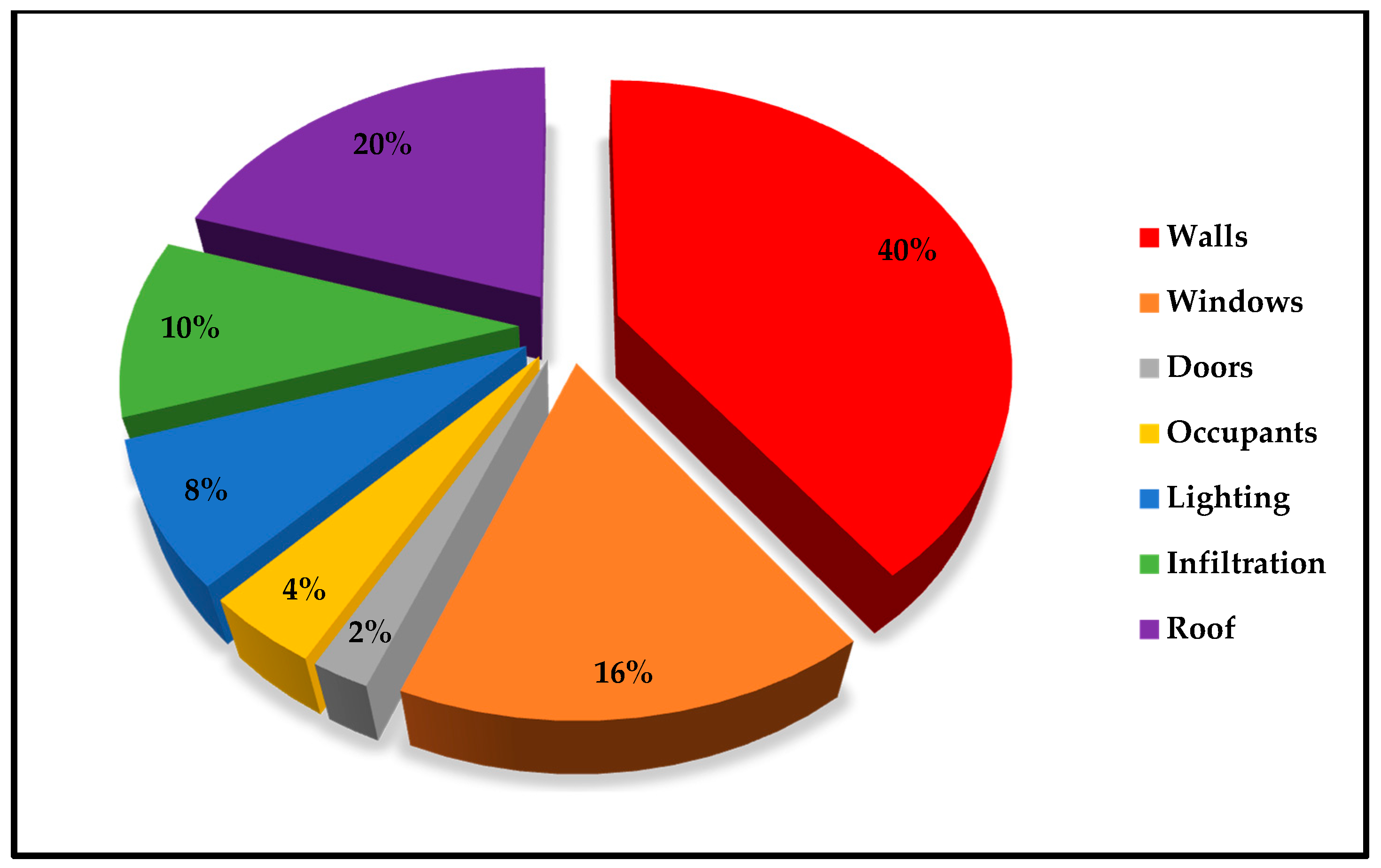
Figure 5.
Diagram of the TRNSYS model of the solar absorption cooling system (SACS).
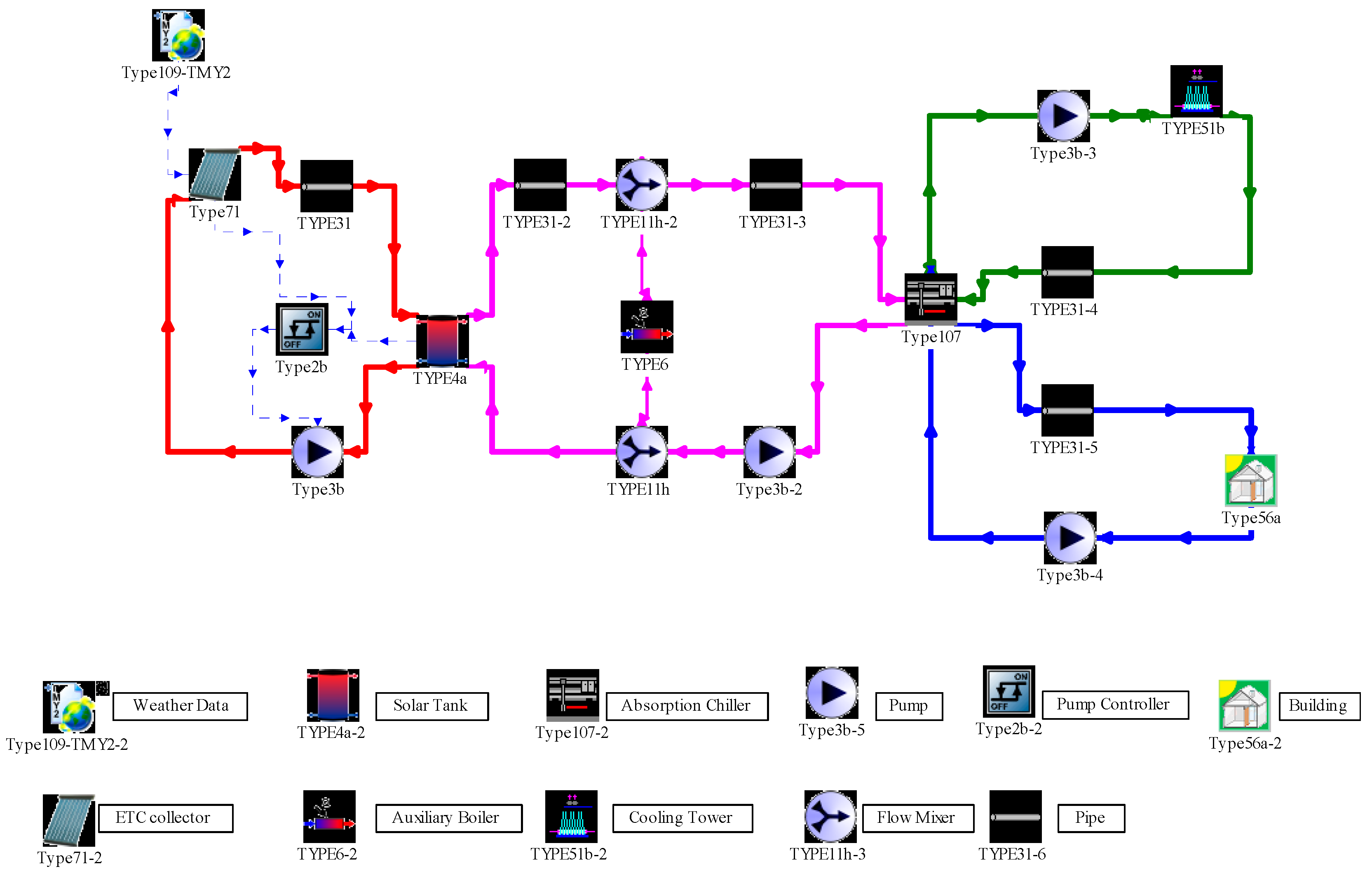
Figure 6.
Energy contribution of integration gas boiler and solar field.

Figure 7.
Solar coverage during cooling season.
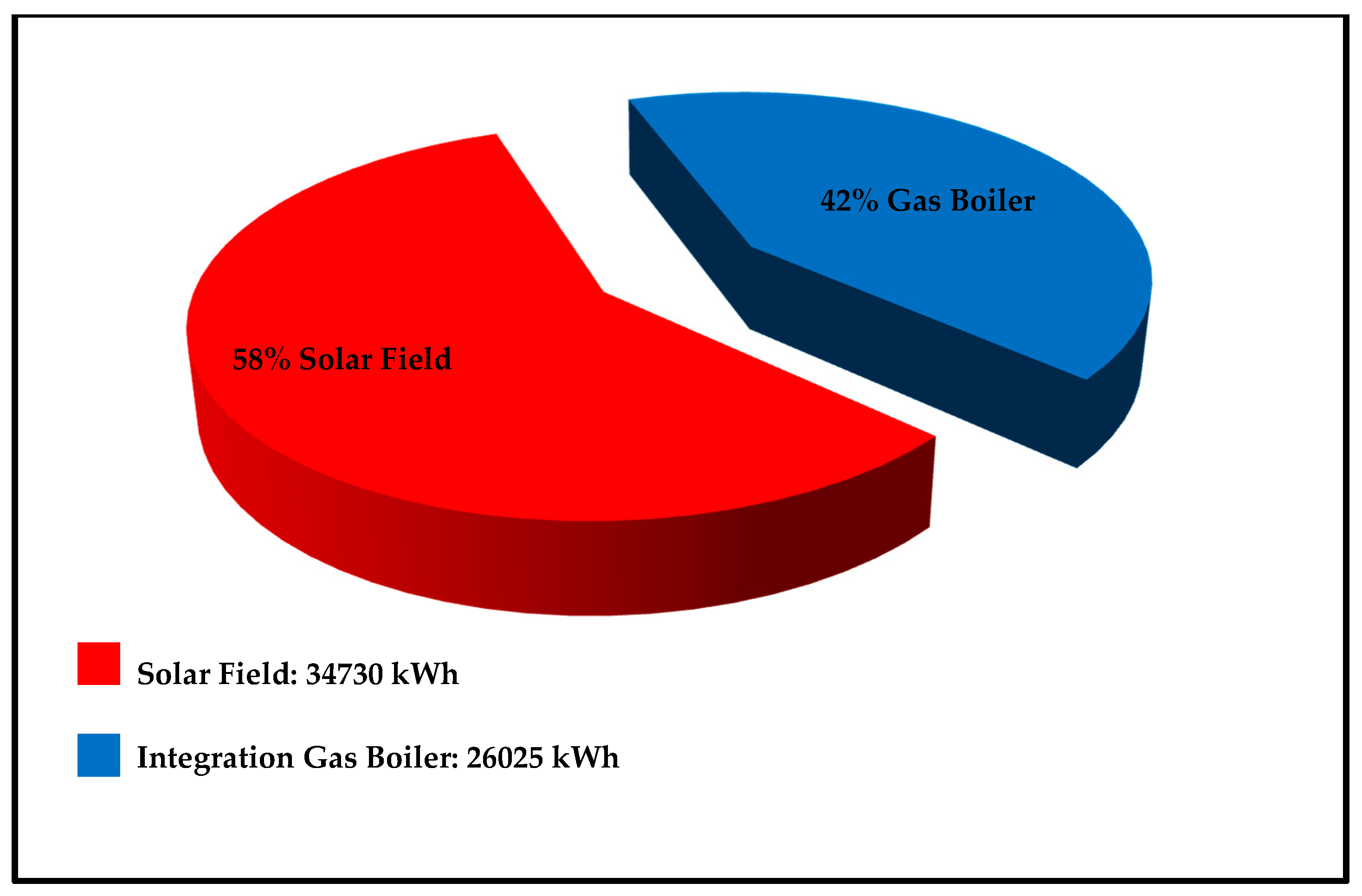
Figure 8.
Energy contribution of solar field and solar tank.

Figure 9.
Solar coverage variation with the solar collector tilt.

Figure 10.
Variation of the solar fraction with the flow of water circulating through the collector.
Figure 10.
Variation of the solar fraction with the flow of water circulating through the collector.

Figure 11.
Solar coverage as a function of the number of collectors.

Figure 12.
Solar coverage as a function of storage tank volume.
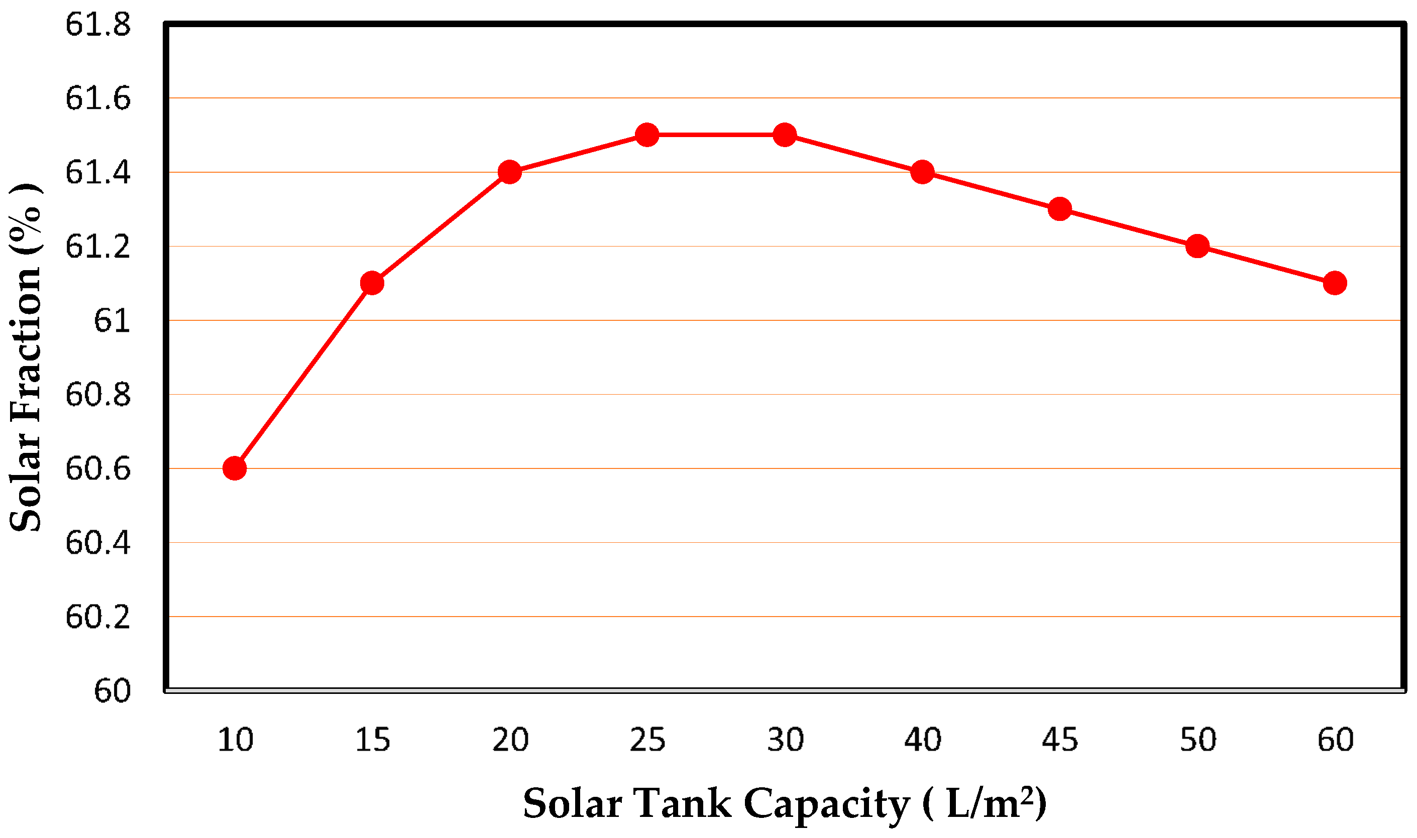
Table 1.
Technical specifications of the Apricus evacuated tube collector (ETC)-30 solar collector [29].
Table 1.
Technical specifications of the Apricus evacuated tube collector (ETC)-30 solar collector [29].
| Variable | Units | Value |
|---|---|---|
| Absorber area | m2 | 2.4 |
| Optical performance () | - | 0.845 |
| Loss coefficient () | W/(m2·K) | 1.47 |
| Loss coefficient () | W/(m2·K) | 0.01 |
Table 2.
Technical characteristics of the FXT-26 cooling tower [32].
Table 2.
Technical characteristics of the FXT-26 cooling tower [32].
| Characteristics | Value | Units |
|---|---|---|
| Cooling tower capacity | 105 | kW |
| Wet temperature | 25 | °C |
| Cooling water temperature | 35-30 | °C |
| Airflow rate | 16 | m3/h |
| Electrical power | 0.75 | kW |
Table 3.
Specifications of the YAZAKI WFC-SC10 absorption chiller [34].
Table 3.
Specifications of the YAZAKI WFC-SC10 absorption chiller [34].
| Characteristic | Unit | Value |
|---|---|---|
| Cooling capacity | kW | 35 |
| Chilled water outlet /inlet temp. | °C | 7/12.5 |
| Cooling water outlet /inlet temp. | °C | 35/31 |
| Heating water outlet /inlet temp. | °C | 88/83 |
| Chilled water flowrate | m3/h | 11 |
| Cooling water flow rate | m3/h | 36.7 |
| Heating water flow rate | m3/h | 17.3 |
| Electric power consumption | kW | 0.21 |
Table 4.
List of the most important components of the TRNSYS model.
| Component | Type TRNSYS | Parameters (Base Design Values) |
|---|---|---|
| Solar Collector | TYPE 71a | Apricus ETC-30 (Table 3) Number of collectors (12) Inclination (30°) |
| Hot water tank | TYPE 4a | Volume (50 L/m2 collector) |
| Auxiliary boiler | TYPE 6 | Efficiency (90%) |
| Absorption chiller | TYPE 107 | YAZAKI WFC SC10 (Table 5) |
| Cooling tower | TYPE 51b | B.A.C. FXT-26 (Table 4) |
| Weather data | TYPE 109—TMY2 | Location: Baghdad, Iraq |
| Collector pump | TYPE 3b | Flow rate 50 (L/h)/m2 of collector |
| Collector pump control | TYPE 2b | Maximum accumulator temperature (90 °C) Minimum collector gain (5 °C) |
| Pipe | TYPE 31 | |
| Flow mixer | TYPE 11h | |
| Building | TYPE 56a |
Table 5.
Most relevant data and results for the cooling season operation (kWh).
| Month | Incident Energy | Collected Energy | Solar Tank Energy | Aux. Boiler Energy | Load Energy | Collector Efficiency (%) | COP | Solar Fraction (%) |
|---|---|---|---|---|---|---|---|---|
| April | 17,329 | 9489 | 2350 | 1760 | 4110 | 54.75 | 0.39 | 57.17 |
| May | 19,624 | 11,346 | 3642 | 1954 | 5596 | 57.81 | 0.41 | 65.08 |
| June | 30,632 | 16,358 | 6243 | 4720 | 10,963 | 53.40 | 0.45 | 56.94 |
| July | 33,685 | 18,509 | 7496 | 5153 | 12,649 | 54.94 | 0.51 | 59.26 |
| August | 35,173 | 19,245 | 7889 | 5391 | 13,280 | 54.71 | 0.52 | 59.40 |
| September | 29,627 | 15,296 | 4948 | 4430 | 9378 | 51.62 | 0.40 | 52.76 |
| Oct. | 11,953 | 5830 | 2162 | 2617 | 4779 | 48.77 | 0.40 | 45.23 |
| Total | 178,023 | 96,073 | 34,730 | 26,025 | 60,755 | 53.96 | 0.44 | 57.16 |
Table 6.
Primary energy performance for various collector areas and solar tank volume.
| Number of Collectors | Solar Tank Volume L | ||||||
|---|---|---|---|---|---|---|---|
| 10 (25 m2) | 12 (30 m2) | 14(35 m2) | 1000 | 1500 | 2000 | ||
| Solar Fraction% | 53.1 | 62.3 | 70.2 | 61.5 | 62.3 | 63.9 | |
| ηele,total | 11.2 | 11.5 | 11.9 | 11.6 | 11.9 | 12.1 | |
| PE save | PEsave kWhPE | 1361 | 3759 | 5661 | 4669 | 5761 | 6342 |
| PEref (Primary Energy References) kWhPE | 15,469 | 15,545 | 15,666 | 15,628 | 15,666 | 15,306 | |
| Relative % | 8.8 | 24.8 | 36.8 | 29.9 | 36.8 | 40.6 | |
Table 7.
Variation of the solar coverage with the lower temperature of the solar tank.
| Temperature °C | 70 | 72.5 | 75 | 77.5 | 80 |
|---|---|---|---|---|---|
| Solar Fraction% | 63.1 | 62.2 | 61.2 | 59.9 | 57.9 |
Table 8.
Variation of solar coverage with an upper temperature of the solar tank.
| Temperature °C | 85 | 87.5 | 90 | 92.5 | 95 |
|---|---|---|---|---|---|
| Solar Fraction% | 60.7 | 61.0 | 61.2 | 61.3 | 60.6 |
© 2020 by the authors. Licensee MDPI, Basel, Switzerland. This article is an open access article distributed under the terms and conditions of the Creative Commons Attribution (CC BY) license (http://creativecommons.org/licenses/by/4.0/).
Share and Cite
MDPI and ACS Style
Al-Falahi, A.; Alobaid, F.; Epple, B. A New Design of an Integrated Solar Absorption Cooling System Driven by an Evacuated Tube Collector: A Case Study for Baghdad, Iraq. Appl. Sci. 2020, 10, 3622. https://doi.org/10.3390/app10103622
AMA Style
Al-Falahi A, Alobaid F, Epple B. A New Design of an Integrated Solar Absorption Cooling System Driven by an Evacuated Tube Collector: A Case Study for Baghdad, Iraq. Applied Sciences. 2020; 10(10):3622. https://doi.org/10.3390/app10103622
Chicago/Turabian StyleAl-Falahi, Adil, Falah Alobaid, and Bernd Epple. 2020. "A New Design of an Integrated Solar Absorption Cooling System Driven by an Evacuated Tube Collector: A Case Study for Baghdad, Iraq" Applied Sciences 10, no. 10: 3622. https://doi.org/10.3390/app10103622
Note that from the first issue of 2016, this journal uses article numbers instead of page numbers. See further details here.