The Levenberg–Marquardt Method for Acousto-Electric Tomography on Different Conductivity Contrast

Abstract

The stability and convergence performance of Levenberg–Marquardt method for acousto-electric tomography (AET) applied to different levels of conductivity contrast is studied in this paper. As a multi-physical imaging modality, acousto-electric tomography (AET) provides high spatial imaging resolution while also conserving the high contrast property of electrical impedance tomography. The Levenberg–Marquardt method is a well known iteration scheme which can be applied for the nonlinear problem of AET. However, the influence of the conductivity contrast on the stability and convergence performances of this conductivity reconstruction method is rarely discussed in the literature. In this paper, the performance of the Tikhonov regularization-based Levenberg–Marquardt method is applied to reconstruct conductivity map with different conductivity contrast between different regions of the domain of interest (DOI). Numerical investigations are carried out for phantoms with different conductivity contrast. Reconstructed results with different levels of noise are presented and discussed in detail.

1. Introduction

Electrical Impedance Tomography (EIT) is a noninvasive technique for reconstructing the conductivity distribution from the measured potential on the electrodes that are attached to the surface of the domain of interest (DOI), and current is injected through the same electrodes into DOI [1]. As the total number of measurements is much smaller than the total number of points to be reconstructed, the EIT problem is severely ill-posed. Acousto-electric tomography [2,3,4,5] is developed to improve the ill-posedness and spatial imaging resolution of electrical impedance tomography (EIT) while conserving the high contrast property of EIT. Other methods, e.g., learning structural sparsity via a Bayesian approach [6,7], and some based on multi-physics models [8,9], exist as well for the same purpose. AET is applied to determine the internal conductivity of a physical body with better stability and resolution compared to the ill-posed EIT. The main idea is to carry out a classical EIT measurement while a known focused ultrasonic wave travels through the DOI. The high intensity of the pressure produced by the acoustic wave creates a small local deformation within the DOI, and this deformation changes the electrical conductivity locally, and therefore the electrical current distribution, which further changes the electric voltages measured on the electrodes. The higher the electrical conductivity in the acoustic wave focal zone, the greater the change. This deformation also influences the resolution of the imaging [2]. The resulting changes of the boundary potential can be recorded with EIT measurements [10], which are then used to compute the power density [2,11] for reconstructing the distribution of conductivity in the DOI. This method also has the potential applications in the materials damage detection [12,13].

The conductivity reconstruction from the power density is an ill-posed nonlinear inverse problem. Many works have been reported for solving it in the existing literature, and many for improving the performance of these algorithms [14,15]. The Levenberg–Marquardt method is a nonlinear optimization method well known for its convergence and stability, and it has been applied to solve the nonlinear problem of AET [14,16,17]. A Tikhonov regularization is used in the computation for better computation performance on stability, noise tolerance and accuracy. The adjoint operators required in the method are computed via constructing several PDEs for reconstructing the conductivity distribution iteratively.

Numerical results presented in [14,16,17] show a good performance of the Levenberg–Marquardt method to different numerical phantoms, but the algorithm has several theoretical requirements to be meet for a stable computational performance, these include a well-chosen regularization parameter, the continuity requirements on the power density, and the existence of the second-order derivative of the conductivity distribution for the computation of the adjoint operator of power density. However, all the above requirements can be coupled together to give a synthesized influence on the performance of the algorithm, and neither the influence of each parameter nor the synthesized influence of all the parameters are discussed in the literature. Especially the contrast of the conductivity between regions of the whole DOI, which can render both conductivity and power density discontinue to violate the continuity requirements on the algorithm, which in turn requires the regularization parameter to be properly chosen. The focus of the present contribution is on the stability of the Levenberg–Marquardt method with respect to the above factors when it is applied to solve the nonlinear AET problem with multi-domain and different levels of conductivity contrasts. Numerical results of the computed power density, convergence performance, and the reconstructed conductivity distribution are presented and investigated in detail based on a simple phantom with two circular domain and more complicated heart–lung model including multiple domains inside.

2. The Reconstruction Algorithm Based on Levenberg–Marquardt Method

2.1. The Inverse Problem and Forward Model

A physical body imaged by EIT is modeled as a bounded Lipschitz domain $\Omega \subset {\mathbb{R}}^n$ for $n\ge 2$. The changes caused by the acoustic wave can be recorded with EIT measurements on boundary $\partial \Omega$ [18,19,20]. The power density in $\Omega$ is defined as

$$\mathcal{E}\left(\sigma \right)={\sigma |\nabla u\left(\sigma \right)|}^2,\Omega \subset {\mathbb{R}}^n.$$

(1)

where $\sigma$ is the conductivity map in domain $\Omega$. $u\left(\sigma \right)$ is the electrical potential produced by applying either voltage or electric current on $\partial \Omega$. Given noisy measurements ${\mathcal{E}}^{\delta }\left(\sigma \right)$ of the true power density $\mathcal{E}\left(\sigma \right)$, the problem is to reconstruct conductivity map $\sigma$ via minimizing the following functional,

$$\underset{\sigma }{min}\left|\right|{\mathcal{E}}^{\delta }\left(\sigma \right)-\mathcal{E}\left(\sigma \right){\left|\right|}_{L^2(\Omega )}.$$

(2)

The power density $\mathcal{E}\left(\sigma \right)$ can be reconstructed from the boundary measurements [2,21]. The nonlinear relationship between $\mathcal{E}\left(\sigma \right)$ and $\sigma$ renders this problem nonlinear [22]. To develop the methods for reconstructing $\sigma$ from $\mathcal{E}\left(\sigma \right)$, the continuum model with Dirichlet condition is used here

$$\begin{array}{cc}\hfill \nabla ·\sigma \nabla u& =0,\mathrm{in}\Omega \hfill \end{array}$$

(3a)

$$\begin{array}{cc}\hfill u& =f,\mathrm{on}\partial \Omega .\hfill \end{array}$$

(3b)

f is the boundary potential, $f\in H^{1/2}(\Omega )$. The present work assumes $\sigma$ is positive. With the assumption that measurements are carried out in the low frequency domain without any interior sources or charges in $\Omega$, Equation (3a) is obtained by simplifying time-harmonic Maxwell’s equation with low-frequency approximation [17].

2.2. The Reconstruction Algorithm

The Levenberg–Marquardt algorithm (LMA) locates the minimum of a function expressed as the sum of squares of errors between function and measured data through iterative updating. For a general operator equation $F\left(\sigma \right)=\mathcal{E}{\left(\sigma \right)}^{\delta }$, where $F:X\to Y$ and X, Y are Hilbert spaces [23]. $\mathcal{E}{\left(\sigma \right)}^{\delta }$ is the measured noisy data of $\mathcal{E}\left(\sigma \right)$. More practically, one could instead minimize [24,25]

$${\sigma }_{k+1}=\underset{\sigma }{min}{∥\mathcal{E}{\left(\sigma \right)}^{\delta }-F\left({\sigma }_k\right)-F^{\prime }\left({\sigma }_k\right)\delta \sigma ∥}_Y^2+{\alpha }_k{∥\delta \sigma ∥}_X^2,$$

(4)

letting ${\alpha }_k$ the Tikhonov regularization parameter, and $\delta \sigma =\sigma -{\sigma }_k$. This minimization problem regarding to (4) is equivalent to the linearized one

$${\sigma }_{k+1}={\sigma }_k+{(F^{\prime }{\left({\sigma }_k\right)}^{*}{F}^{\prime }\left({\sigma }_k\right)+{\alpha }_k)}^{-1}{F}^{\prime }{\left({\sigma }_k\right)}^{*}(\mathcal{E}{\left(\sigma \right)}^{\delta }-F\left({\sigma }_k\right)),$$

(5)

letting $F^{\prime }{\left({\sigma }_k\right)}^{*}$ the adjoint of $F^{\prime }\left({\sigma }_k\right)$. It has been proven in [17,26,27,28,29], with a properly chosen parameter ${\alpha }_k$ and an initial guess ${\sigma }_0$ sufficiently close to the desired solution, that the LMA converges to a solution ${\sigma }^{\delta }$ of $F\left({\sigma }^{\delta }\right)=\mathcal{E}{\left(\sigma \right)}^{\delta }$.

The LMA based on Equation (5) can be thought of as a combination of steepest descent and Gauss–Newton method. When the current solution is far from the correct one, a large value is given to ${\alpha }_k$, and LMA behaves like a steepest-descent method, which converges slowly but well. When the current solution is close to the correct solution, a small ${\alpha }_k$ is used, and LMA behaves like a Gauss–Newton method which is known as a faster iterative method than the steepest descent. The Fréchet derivative and adjoint operator needed in (5) are computed with a method proposed in [17], as follows. It is assumed that $\sigma$ is positive, and $\sigma \in {\mathcal{H}}^l(\Omega )$ for $l>n/2$. For $f\in {\mathcal{H}}^{l+\frac{1}{2}}(\Omega )$, then the forward model has a unique solution $u\left(\sigma \right)\in {\mathcal{H}}^{l+1}(\Omega )$, which indicates the operators $\mathcal{E}\left(\sigma \right)$, ${\mathcal{E}}^{\prime }\left(\sigma \right)$, and ${\mathcal{E}}^{\prime }{\left(\sigma \right)}^{*}$ are all maps from ${\mathcal{H}}^s(\Omega )$ to ${\mathcal{H}}^s(\Omega )$ [17].

If $u^{\prime }\left(\sigma \right)$ is the Fréchet derivative of $u\left(\sigma \right)$ in $\Omega$,

$$u(\sigma +\tau )=u\left(\sigma \right)+u^{\prime }\left(\sigma \right)\tau +o\left(\tau \right)$$

(6)

is established for $\tau \to 0$. $o\left(\tau \right)$ is the remainder. Define $L_{\sigma }\left(u\right)=u\to \nabla ·(\sigma \nabla u)$. According to Equations (3a) and (6),

$$L_{\sigma }{u}^{\prime }\left(\sigma \right)\tau +\nabla ·(\tau \nabla u\left(\sigma \right))=0.$$

(7)

The boundary conditions for $u^{\prime }\left(\sigma \right)\tau$ can also be derived from Equation (6). If $\xi =u^{\prime }\left(\sigma \right)\tau$, then $\xi$ satisfies

$$\begin{array}{cc}\hfill \nabla ·\sigma \nabla \xi +\nabla ·(\tau \nabla u(\sigma \left)\right)& =0,\mathrm{in}\Omega ,\hfill \end{array}$$

(8a)

$$\begin{array}{cc}\hfill \xi & =0,\mathrm{on}{e}_l.\hfill \end{array}$$

(8b)

Here, it is assumed that $\tau$ vanishes in a domain ${\Omega }_{ϵ}=\{x\in \overline{\Omega }|d(x,\partial \Omega )<ϵ\}$ for a sufficiently small $ϵ$. Therefore, all terms regarding to $\tau$ in the boundary conditions disappear. It is well known that the solution of Equations (8) uniquely exists in a weak sense. $u^{\prime }\left(\sigma \right)$ as defined in (8) is the Fréchet derivative of $u\left(\sigma \right)$.

The directional derivative of $\mathcal{E}\left(\sigma \right)$ is given as

$${\mathcal{E}}^{\prime }\left(\sigma \right)\tau \approx \mathcal{E}(\sigma +\tau )-\mathcal{E}\left(\sigma \right)\approx \tau {|\nabla u\left(\sigma \right)|}^2+2\sigma \nabla u\left(\sigma \right)\nabla \xi$$

(9)

with terms of the order of ${\parallel \tau \parallel }^2$ neglected. ${\mathcal{E}}^{\prime }\left(\sigma \right)\tau$ is actually the Fréchet derivative of $\mathcal{E}\left(\sigma \right)$.

Let us assume $\Omega \subset {\mathbb{R}}^2$ for simplicity, and consider the effect of noise. The latter cannot be assumed to be differentiable, then $\mathcal{E}\left(\sigma \right):{\mathcal{H}}^2(\Omega )\to {\mathcal{L}}^2(\Omega )$. As ${\mathcal{E}}^{\prime }\left(\sigma \right):{\mathcal{H}}^2(\Omega )\to {\mathcal{L}}^2(\Omega )$ is a bounded operator, its Hilbert adjoint ${\mathcal{E}}^{\prime }{\left(\sigma \right)}^{*}:{\mathcal{L}}^2(\Omega )\to {\mathcal{H}}^2(\Omega )$ is bounded as well [30]. With embedding operator $B:{\mathcal{H}}^2(\Omega )\to {\mathcal{L}}^2(\Omega )$, ${\mathcal{E}}^{\prime }{\left(\sigma \right)}^{*}$ can be written as

$$\begin{array}{cc}\hfill & {\mathcal{E}}^{\prime }{\left(\sigma \right)}^{*}:{\mathcal{L}}^2(\Omega )\to {\mathcal{H}}^2(\Omega ),\hfill \end{array}$$

(10)

$$\begin{array}{cc}\hfill & {\mathcal{E}}^{\prime }{\left(\sigma \right)}^{*}z=B^{*}{\tilde{\mathcal{E}}}^{\prime }{\left(\sigma \right)}^{*}z.\hfill \end{array}$$

(11)

${\tilde{\mathcal{E}}}^{\prime }{\left(\sigma \right)}^{*}$ is the ${\mathcal{L}}^2(\Omega )$-adjoint of ${\mathcal{E}}^{\prime }\left(\sigma \right)$. $z\in {\mathcal{L}}^2(\Omega )$, and ${\tilde{\mathcal{E}}}^{\prime }{\left(\sigma \right)}^{*}z={|\nabla u\left(\sigma \right)|}^{2}z+2\nabla u\nabla Vz$. The map $V:{\mathcal{H}}^2(\Omega )\to {\mathcal{H}}^2(\Omega )$ is linear and defined by

$$\begin{array}{cc}\hfill L_{\sigma }Vz& =-\nabla ·(z\sigma \nabla u(\sigma \left)\right)\mathrm{in}\Omega ,\hfill \end{array}$$

(12a)

$$\begin{array}{cc}\hfill Vz& =0\mathrm{on}\partial \Omega .\hfill \end{array}$$

(12b)

If multiple measurements are considered, ${\tilde{\mathcal{E}}}_H^{\prime }{\left(\sigma \right)}^{*}z$ in Equation (11) is replaced with ${\tilde{\mathcal{E}}}^{\prime }\left(\sigma \right)$ defined as

$${\tilde{\mathcal{E}}}^{\prime }{\left(\sigma \right)}^{*}z=B^{*}\sum _{i=1}^M\left(\right|\nabla u_i\left(\sigma \right){|}^2{z}_i+2\nabla u_i\nabla V{z}_i)$$

(13)

To calculate $B^{*}:{\mathcal{L}}^2(\Omega )\to {\mathcal{H}}^2(\Omega )$, we allow

$$\sigma \in H_0^2(\Omega )=\left\{x\in {\mathcal{H}}^2(\Omega ):\frac{\partial x}{\partial \nu }=0\right\}$$

(14)

with its inner product given as

$${\langle x,y\rangle }_{{\mathcal{H}}^2(\Omega )}={\langle x,y\rangle }_{{\mathcal{L}}^2(\Omega )}+{\beta }^2{\langle \Delta x,\Delta y\rangle }_{{\mathcal{L}}^2(\Omega )}.$$

(15)

$\beta$ is a regularization parameter, which enforces a second-order weak derivative. Upon integration by parts, $B^{*}\zeta$ is the solution of the Neumann problem

$$\begin{array}{cc}\hfill (Id+{\beta }^2\Delta \Delta )B^{*}\varsigma & =\varsigma ,\hfill \end{array}$$

(16a)

$$\begin{array}{cc}\hfill \frac{\partial \Delta B^{*}\varsigma }{\partial \nu }& =0,\mathrm{on}\partial \Omega \hfill \end{array}$$

(16b)

$$\begin{array}{cc}\hfill \frac{\partial B^{*}\varsigma }{\partial \nu }& =0,\mathrm{on}\partial \Omega \hfill \end{array}$$

(16c)

with $\varsigma \in {\mathcal{L}}^2(\Omega )$. Refer to the work in [17] for more detail. This fourth-order partial differential equation is not practical, but it can be written into an equivalent form

$$\begin{array}{cc}\hfill B^{*}\varsigma +{\beta }^2\Delta \chi & =\varsigma ,\hfill \end{array}$$

(17a)

$$\begin{array}{cc}\hfill \chi -\Delta B^{*}\varsigma & =0,\hfill \end{array}$$

(17b)

$$\begin{array}{cc}\hfill \frac{\partial \chi }{\partial \nu }& =0,\mathrm{on}\partial \Omega \hfill \end{array}$$

(17c)

$$\begin{array}{cc}\hfill \frac{\partial B^{*}\varsigma }{\partial \nu }& =0,\mathrm{on}\partial \Omega \hfill \end{array}$$

(17d)

According to the Levenberg–Marquardt iteration in Equation (5), the formula for calculating the k-th updating step ${\tau }_k$ for the problem at hand is given as

$$({\mathcal{E}}^{\prime }{\left({\sigma }_k\right)}^{*}{\mathcal{E}}^{\prime }\left({\sigma }_k\right)+{\alpha }_{k}Id){\tau }_k={\mathcal{E}}^{\prime }{\left({\sigma }_k\right)}^{*}({\mathcal{E}}^{\delta }-\mathcal{E}\left({\sigma }_k\right)),$$

(18)

where ${\mathcal{E}}^{\delta }$ represents the measured power density derived from $u_b$ and $u_{b,ϵ}$ in the last section. For the left hand side of (18), ${\mathcal{E}}^{\prime }{\left({\sigma }_k\right)}^{*}{\mathcal{E}}^{\prime }\left({\sigma }_k\right)\tau =B^{*}M\tau$ with

$$\begin{array}{cc}\hfill M\tau =& {|\nabla u|}^2{(\tau |\nabla u|}^2+2\sigma \nabla u\nabla u^{\prime }{(\sigma )\tau )+2\nabla u\nabla V(\tau |\nabla u|}^2)\hfill \\ \hfill & +4\nabla u\nabla V(\sigma \nabla u\nabla u^{\prime }\left(\sigma \right)\tau ).\hfill \end{array}$$

(19)

Here, $M\tau$ is easily obtained with Equations (9) and (11). After computing ${\tau }_k$ from (18), the conductivity map ${\sigma }_k$ obtained at the k-th iteration is updated by ${\sigma }_{k+1}={\sigma }_k+{\tau }_k$ for a new iteration. To calculate $B^{*}M\tau$, Equation (17) needs to be solved with $\varsigma =M\tau$, which requires first solving Equations (8) and (12). As all these PDE systems are coupled to each other via $\tau$, they need to be collected into one PDE system and solved in one variational form.

It yields the following system,

$$\begin{array}{cc}\hfill \varphi +{\alpha }_k{\tau }_k=y,& \mathrm{in}\Omega ,\hfill \end{array}$$

(20a)

$$\begin{array}{cc}\hfill \Delta \varphi -\chi =0,& \mathrm{on}\partial \Omega ,\hfill \end{array}$$

(20b)

$$\begin{array}{cc}\hfill {\beta }^2\Delta \chi +\varphi -\gamma =0,& \mathrm{on}\partial \Omega ,\hfill \end{array}$$

(20c)

$$\begin{array}{cc}\hfill \partial \varphi /\partial \nu =0,& \mathrm{on}\partial \Omega \hfill \end{array}$$

(20d)

$$\begin{array}{cc}\hfill \partial \chi /\partial \nu =0,& \mathrm{on}\partial \Omega \hfill \end{array}$$

(20e)

$$\begin{array}{cc}\hfill \gamma -M\tau =0,& \mathrm{in}\Omega ,\hfill \end{array}$$

(20f)

$$\begin{array}{cc}\hfill \nabla ·(\sigma +\tau )\nabla \xi +\nabla ·(\tau \nabla u(\sigma \left)\right)=0,& \mathrm{in}\Omega ,\hfill \end{array}$$

(20g)

$$\begin{array}{cc}\hfill \xi =0,& \mathrm{on}\partial \Omega ,\hfill \end{array}$$

(20h)

$$\begin{array}{cc}\hfill L_{\sigma }\rho +\nabla ·({\mathsf{\Phi }}_{ϵ}{\left(\tau \right|\nabla u|}^2)\sigma \nabla u\left(\sigma \right))=0,& \mathrm{in}\Omega ,\hfill \end{array}$$

(20i)

$$\begin{array}{cc}\hfill \rho =0,& \mathrm{on}\partial \Omega \hfill \end{array}$$

(20j)

$$\begin{array}{cc}\hfill L_{\sigma }\kappa +\nabla ·({\mathsf{\Phi }}_{ϵ}(\sigma \nabla u\nabla \xi )\sigma \nabla u\left(\sigma \right))=0,& \mathrm{in}\Omega ,\hfill \end{array}$$

(20k)

$$\begin{array}{cc}\hfill \kappa =0,& \mathrm{on}\partial \Omega .\hfill \end{array}$$

(20l)

with $y={\mathcal{E}}^{\prime }{\left({\sigma }_k\right)}^{*}({\mathcal{E}}^{\delta }-\mathcal{E}\left({\sigma }_k\right))$, $\varphi =B^{*}M\tau$, $\rho =V\left(\tau \right|\nabla u{|}^2)$, and $\kappa =V(\sigma \nabla u\nabla u^{\prime }\left(\sigma \right)\tau )$. If the number of measurements $N>1$, $y=\mathcal{E}{\left({\sigma }_k\right)}^{*}({\mathcal{E}}^{\delta }-\mathcal{E}\left({\sigma }_k\right))$ and $\gamma ={\sum }_n^N{M}_n\tau$ with

$$\begin{array}{cc}\hfill M_n\tau =& |\nabla u_n{|}^2\left(\tau \right|\nabla u_n{|}^2+2\sigma \nabla u_n\nabla {\xi }_n)\hfill \\ \hfill & +2\nabla u_n\nabla {\zeta }_n+4\nabla u_n\nabla {\kappa }_n\hfill \end{array}$$

(21)

Equations (20g)–(20l) must be solved for each measurement, so one additional measurement will require to solve in addition three partial differential equations. The smoothness requirement on $\sigma$ can be achieved by a so-called mollification operation. To solve the above system, ${\mathcal{E}}^{\prime }{\left({\sigma }_k\right)}^{*}({\mathcal{E}}^{\delta }-\mathcal{E}\left({\sigma }_k\right))$ is needed first. Let $g={\mathcal{E}}^{\delta }-\mathcal{E}\left({\sigma }_k\right)$, then ${\mathcal{E}}^{\prime }{\left({\sigma }_k\right)}^{*}g=B^{*}z$ with $z={|\nabla u|}^2{\mathsf{\Phi }}_{ϵ}g+2\nabla u\nabla w$ and $h=V{\mathsf{\Phi }}_{ϵ}g$. Thus, w can be calculated with (12), and $x=B^{*}z$ is the solution of (17).

The iterative construction method based on the above system is named as LM-CM, referring to Algorithm 1 for a single measurement. As $\nu \left(x\right)$ is not known for the current numerical study, the data of ${\mathcal{E}}^{\delta }$ are simulated by solving (3a) with a Dirichlet boundary condition $u=u_b$ in the present contribution. The relative error $\eta$ is defined as $\eta =\parallel {\sigma }_t-{\sigma }_r{\parallel }_{L_2}/{\parallel {\sigma }_t\parallel }_{L_2}$. Index t indicates the true value, and r means retrieved value. The parameter ${\alpha }_k$ should be updated according to the value of ${\tau }_k$. If ${\sigma }_k+{\tau }_k$ leads to a reduction of the relative error in ${\sigma }_k$, ${\alpha }_k$ is decreased and ${\tau }_k$ is accepted. Otherwise, ${\tau }_k$ is discarded and ${\alpha }_k$ is increased. As $\eta$ cannot be determined in practice, a relatively large value can be given to ${\alpha }_0$, and ${\alpha }_k$ is slowly decreased to ensure convergence. The iteration is stopped when ${∥{\tau }_k∥}_{L_2}$ is smaller than the expected error or the maximum number of iterations is reached.

Algorithm 1 LM-CM algorithm for retrieving the conductivity map of a domain $\Omega$ from a single measurement of power density.

Data: Measured power density ${\mathcal{E}}^{\delta }$ and initial guess ${\sigma }_0$ Result: Retrieved conductivity map ${\sigma }_r$ with relative error $\eta$ 1  N: maximum number of iterations; 2  ${\sigma }_k\leftarrow {\sigma }_0$; 3  ${\alpha }_k\leftarrow {\alpha }_0$; 4  $num\leftarrow 1$; 5  $norm\leftarrow 1$;

3. Numerical Investigations

The conductivity distribution can be obtained from the power density $\mathcal{E}\left(\sigma \right)$ with Algorithm 1 based on the Levenberg–Marquardt method. In the following computation, $\mathcal{E}\left(\sigma \right)$ is computed directly from its definition ${\sigma |\nabla u|}^2$, where u is obtained with the forward model introduced in Section 2.

Different phantoms with different contrast between the inclusion and the background are studied here. The weak forms of the equations in (20) can be easily obtained by applying integration by parts, and the equations are solved with finite element method implemented by using the open-source finite element library FEniCS [31]. Two boundary conditions with $f_1(x,y)=x$ and $f_2(x,y)=y$ are given to Equation (3a) for a reconstruction with multiple measurements. A relative error $\eta$ is defined as $\eta =\parallel {\sigma }_t-{\sigma }_r{\parallel }_{L_2}/{\parallel {\sigma }_t\parallel }_{L_2}$ to indicate the convergence of the Levenberg–Marquardt iteration. Index t indicates the true value, and index r means retrieved value.

Practical measurements are always affected by various noises introduced by the devices or during the measurement process. Here the performance of the algorithm to different levels of contrast is investigated with different levels of noise. The noise level is measured with signal-to-noise ratio (SNR), which is defined as

$$\mathrm{SNR}=20{log}_{10}\frac{\parallel {\mathcal{E}}_p{\parallel }_{L_2}}{{\parallel \mathcal{N}\parallel }_{L_2}},$$

(22)

where $\mathcal{N}$ satisfies Gaussian white noise distribution. The noise is added to the data of $\mathcal{E}\left(\sigma \right)$ for numerical examples with SNR = ∞, 40 dB, and 20 dB. SNR = ∞ for noise free.

3.1. Numerical Study with a Simple Phantom

A phantom with a smaller circular inclusion included in a circular domain is used here for numerically studying the performance of the Levenberg–Marquardt method to various conductivity contrast. The radius of the circular DOI is $1.0 \mathrm{m}$. The circular inclusion with its center located at (−0.3, 0.3) has a radius of $0.2 \mathrm{m}$. The conductivities of the background and the inclusion are denoted as ${\sigma }_b$ and ${\sigma }_i$, respectively. The contrast of the conductivity is defined as ${\sigma }_i/{\sigma }_b$. ${\alpha }_k$ for the k-th iteration is set as ${\alpha }_k={\alpha }_0/a^k$ with ${\alpha }_0=1.0$, $a=2.0$, and ${\beta }_k$ set as constant ${\beta }_0=1\times {10}^{-3}$.

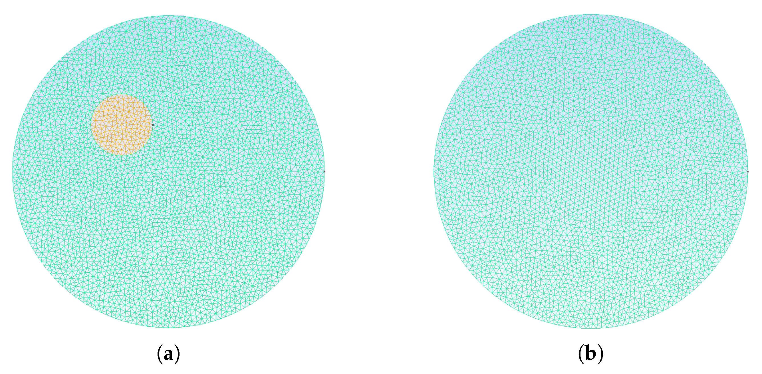
The mesh for the forward model is shown in Figure 1a which has 3854 vertices and 7522 cells. A different mesh, as shown in Figure 1b, with 3671 vertices and 7156 cells is used to avoid inverse crime. The background conductivity is set to $2.0 \mathrm{S}/\mathrm{m}$, and the one for the inclusion is set to a series of values listed as $4.0 \mathrm{S}/\mathrm{m}$, $6.0 \mathrm{S}/\mathrm{m}$, $8.0 \mathrm{S}/\mathrm{m}$, $10.0 \mathrm{S}/\mathrm{m}$, $12.0 \mathrm{S}/\mathrm{m}$, $14.0 \mathrm{S}/\mathrm{m}$, $16.0 \mathrm{S}/\mathrm{m}$, and $18.0 \mathrm{S}/\mathrm{m}$. Therefore, the contrast varies from $2.0$ to $9.0$.

3.2. The Influences of ${\alpha }_k$ and ${\beta }_k$

The different value of ${\alpha }_k$ and ${\beta }_k$ may provide a better contrast of the Levenberg–Marquardt method. Here, the parameters ${\alpha }_0$ and ${\beta }_0$ will be discussed. The conductivity of background is set as $2.0 \mathrm{S}/\mathrm{m}$. The conductivity of interior domain is set as $10.0 \mathrm{S}/\mathrm{m}$, $12.0 \mathrm{S}/\mathrm{m}$, and $14.0 \mathrm{S}/\mathrm{m}$. Two noise levels (SNR = 40 dB, 20 dB) are considered.

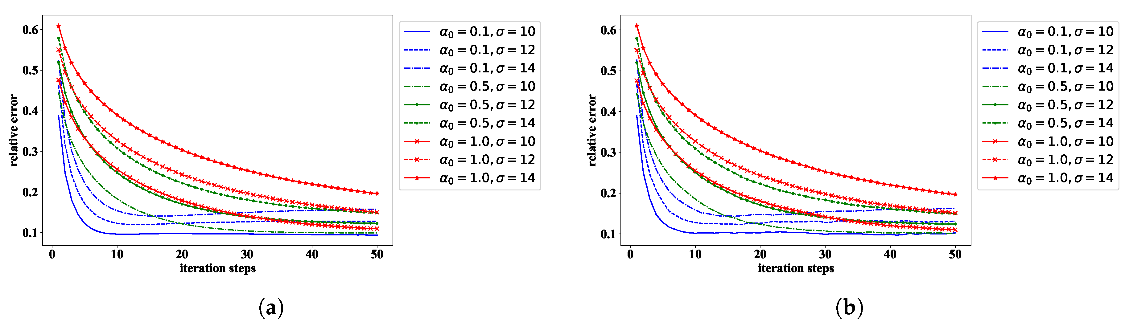
The parameter ${\alpha }_0$ is first set as a constant with 0.1, 0.5, 1.0 while ${\beta }_k=1\times {10}^{-3}$. The variation of the relative error with the iteration for different values of ${\alpha }_0$ is given in Figure 2. In the computation, each iteration takes ~5 s, the whole 50 iterations can be finished in about 5 min.

When ${\alpha }_0=0.1$, the results given in Figure 2a show that the method can converge fast for both low and high contrast cases. However, the relative errors for the high contrast cases, e.g., $\sigma =12.0 \mathrm{S}/\mathrm{m}$, $14.0 \mathrm{S}/\mathrm{m}$, start to diverge after achieving to the minimum relative error. This divergence becomes severe when the noise level is increased, as shown in Figure 2b. When the value of ${\alpha }_0$ is increased, the divergence phenomenon disappear for both lower and higher noisy cases, but the speed of convergence slows down, and it takes much more iteration steps for the computations to achieve a similar level of relative error as ${\alpha }_0=0.1$. A direct comparison of the results is given in Figure 2a,b. A larger value of ${\alpha }_0$ brings higher stability even with higher noise. Therefore, a smaller ${\alpha }_0$ will accelerate the convergence of the computation, and a larger ${\alpha }_0$ will improve the noise tolerance and the performance of the method for high contrast conductivity distribution. To accelerate the convergence without losing the stability of the computation, ${\alpha }_k$ for the k-th iteration is set as ${\alpha }_k={\alpha }_0/a^k$ with ${\alpha }_0=1.0$, $a=2.0$.

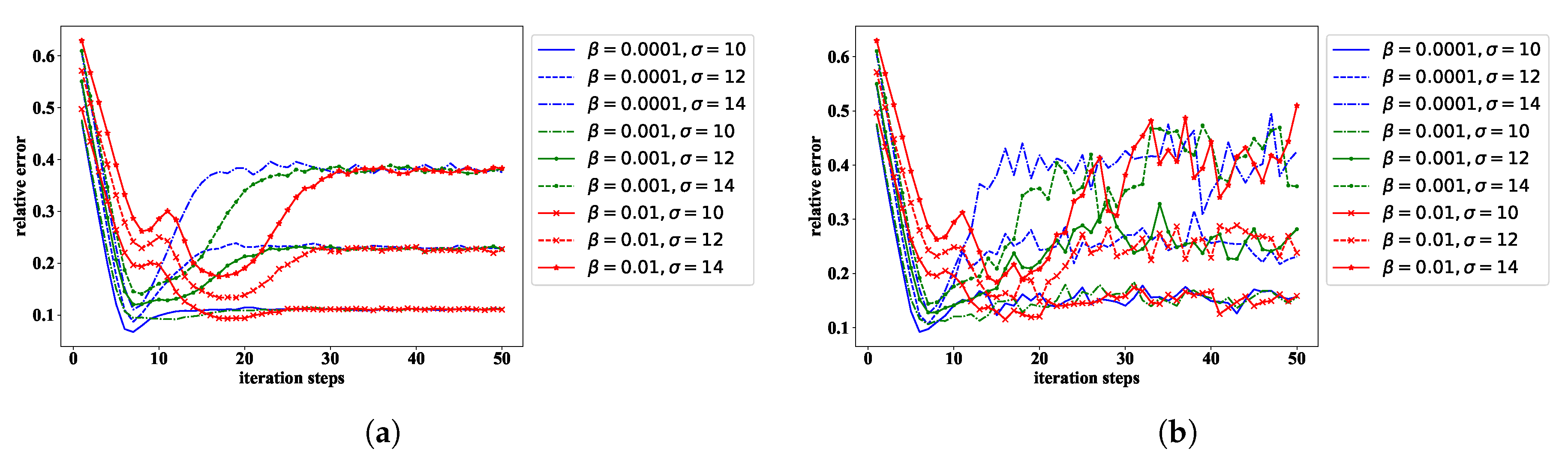
The values of ${\beta }_k={\beta }_0$ are fixed in the following computations. However, a different value of ${\beta }_0$ is possible to provide different performance of the Levenberg–Marquardt method for high contrast cases. The model with two different levels of noise (SNR = 40 dB, 20 dB) will be considered when conductivity is $10.0 \mathrm{S}/\mathrm{m}$, $12.0 \mathrm{S}/\mathrm{m}$, and $14.0 \mathrm{S}/\mathrm{m}$. The ${\beta }_0$ is set as 0.0001, 0.001, and 0.01. The results are shown in Figure 3a,b. When the value of $\beta$ is increased from $0.0001$ to $0.001$, the speed of convergence is similar, this indicates the convergence is mainly dominated by the value of ${\alpha }_k$. However, the minimum relative error achieved during the iteration process is decreased. For the high contrast case, the instability is also influenced by the value of the ${\beta }_k$, a larger ${\beta }_k$ with a better stability, and this becomes more obvious when more noise is introduced into the measured data, as shown in Figure 3b. Therefore, a smaller ${\beta }_0$ will make the minimum relative error smaller during computation, however it decreases the noise tolerance. Therefore, the value of ${\beta }_k$ is set to ${\beta }_0=1\times {10}^{-3}$ in the following computations. The values of ${\beta }_0$ and ${\alpha }_0$ could be greater or smaller whether needed. Another phenomenon observed in Figure 3a,b is that when ${\alpha }_k$ becomes very small, the relative error for the high contrast cases starts to increase, and it stops at certain level. This is the instability caused by the high contrast of the conductivity. Therefore, the value of ${\alpha }_k$ can not be too small. In what follows, the variation of ${\alpha }_k$ follows ${\alpha }_k={\alpha }_0/a^k$ at the beginning of the iteration, but it is fixed to the value where the minimum relative error is achieved.

3.2.1. Numerical results with SNR = ∞

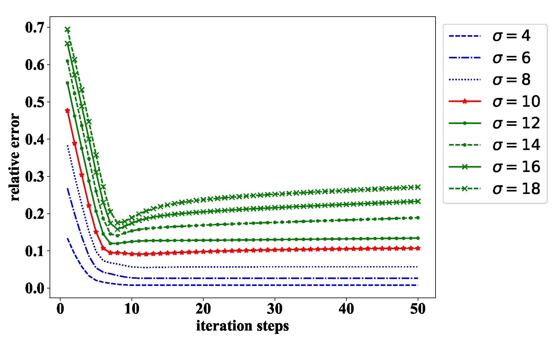
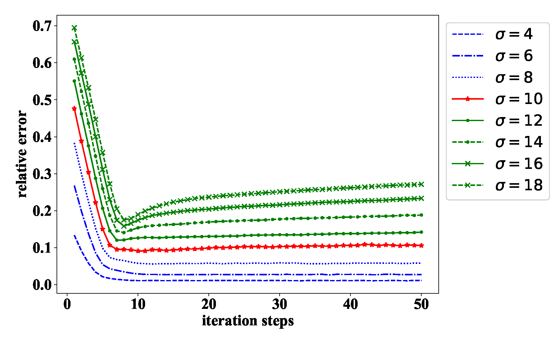
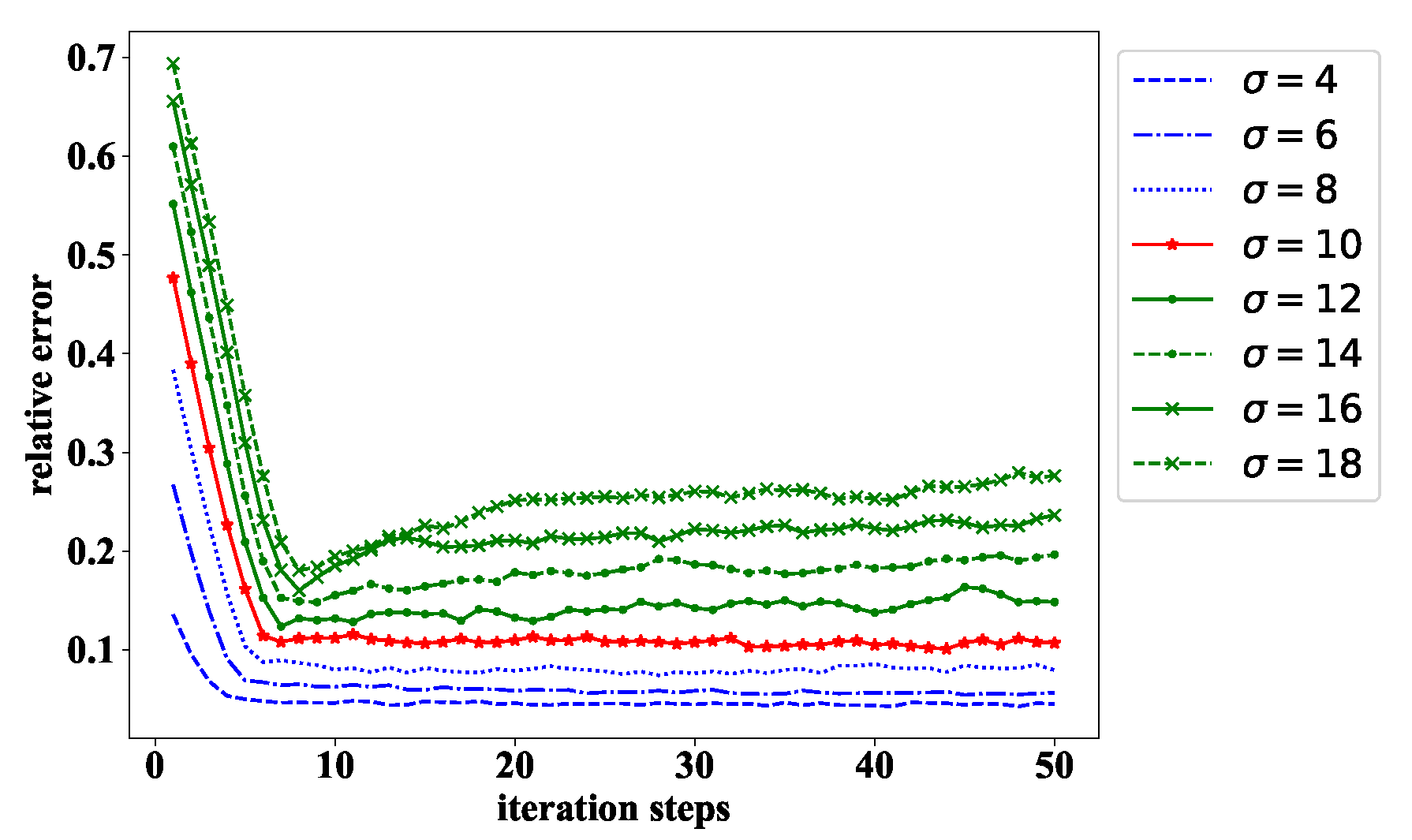
When SNR = ∞, the relative error corresponding to each conductivity is shown in Figure 4. Here, ${\alpha }_k$ for the k-th iteration is set as ${\alpha }_k={\alpha }_0/a^k$ with ${\alpha }_0=1.0$ and $a=2.0$, and ${\beta }_k$ is set as constant ${\beta }_0=1\times {10}^{-3}$. The figure shows that the algorithm works stably with good convergence when the conductivity ${\sigma }_i$ is less than $10.0 \mathrm{S}/\mathrm{m}$, where the contrast is 5. When the contrast is more than 5, the algorithm converges to certain level, and then it starts to diverge. The curve of the relative error varying with iteration steps becomes a “V-shape”. The minimum relative error becomes larger as the contrast increases, as obviously seen in Figure 4. This phenomenon is also observed in Figure 3a for high contrast cases and Figure 3b for almost all the noisy cases. Theoretically, the conductivity distribution should be in the $H^2(\Omega )$ space, and the value of ${\beta }_k$ is closely related to the second order derivative of the conductivity distribution as shown in Equation (15). When the contrast is too high, this continuity requirement can not be satisfied, this “V-shape” curve of the relative error appears.

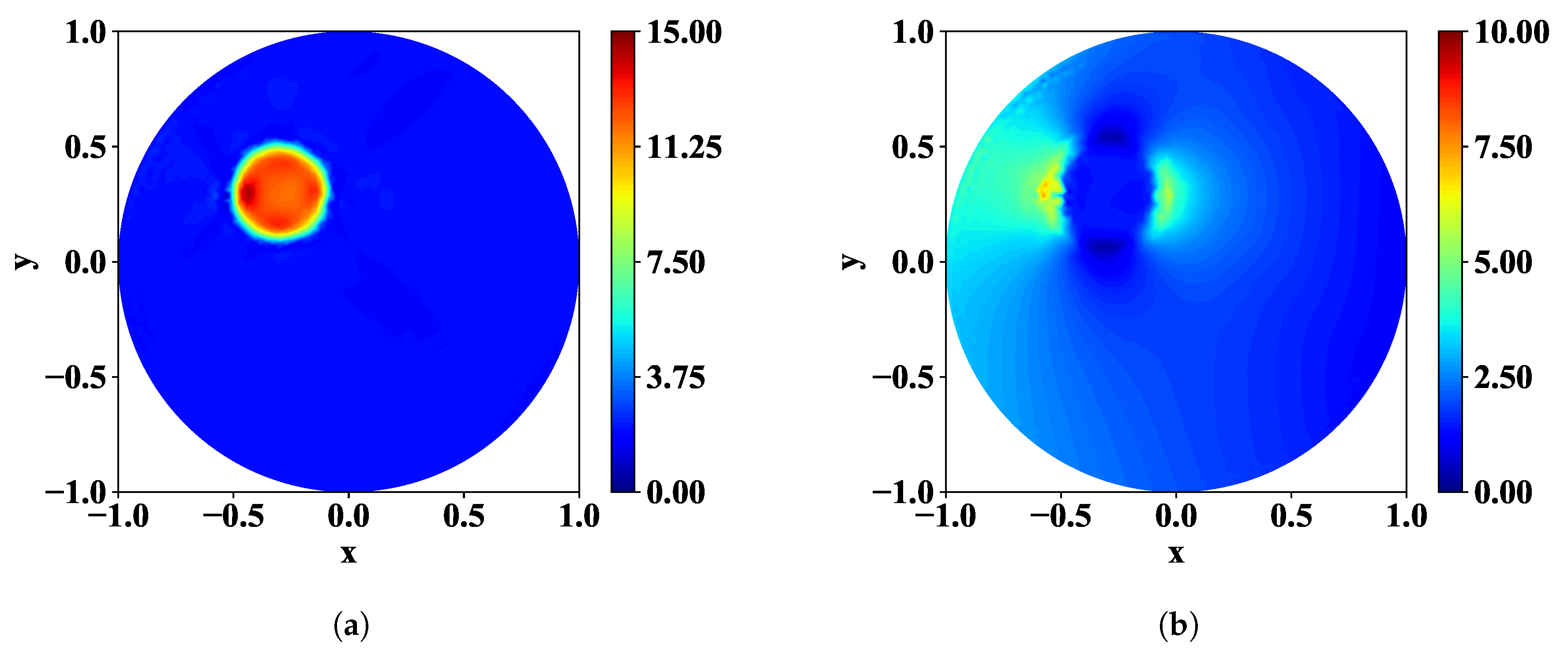
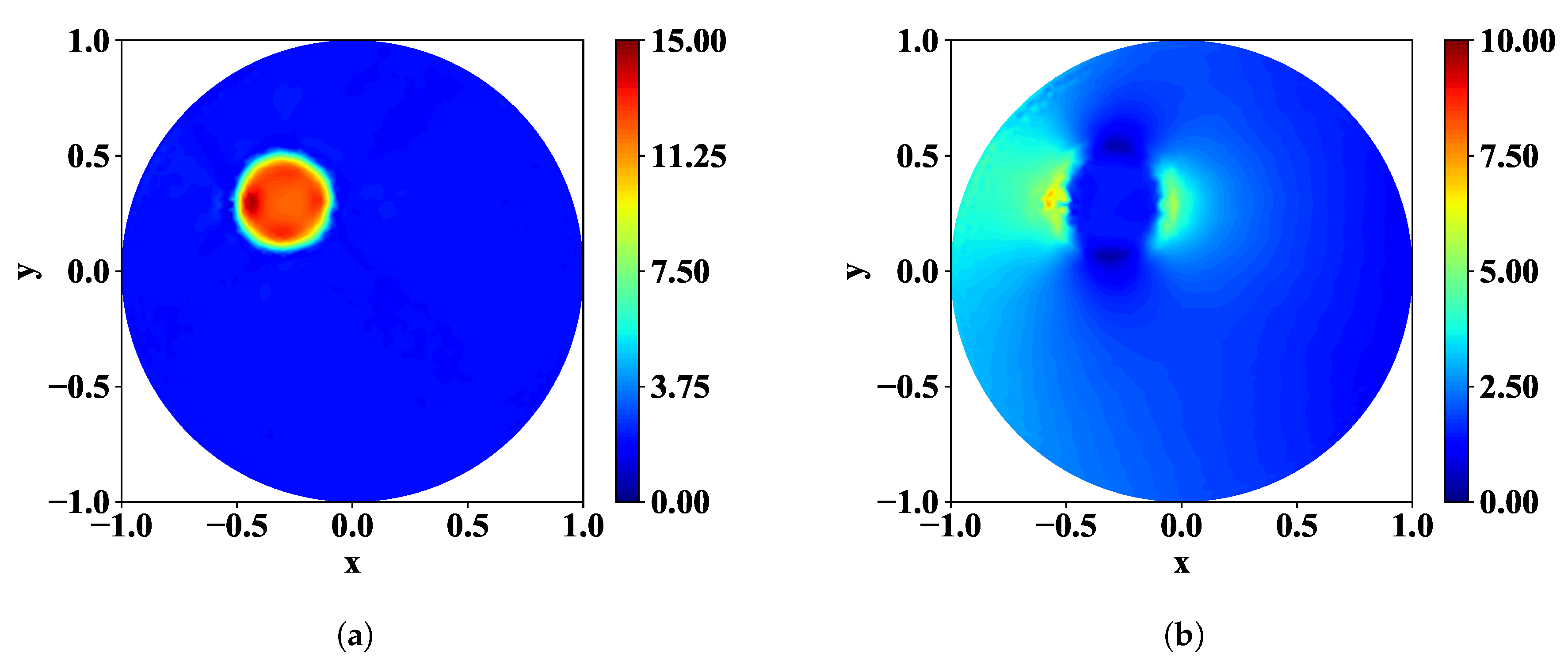
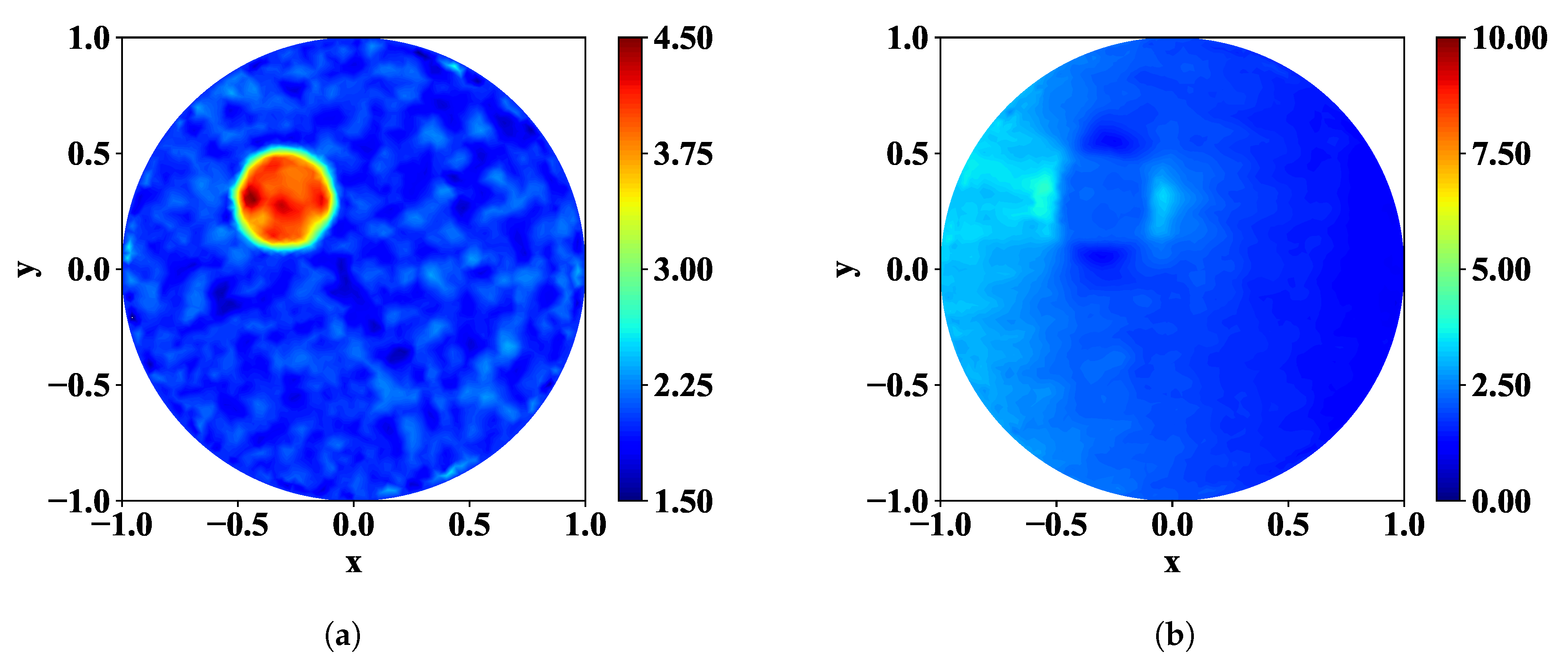
When the conductivity of the inclusion is ${\sigma }_i=4.0 \mathrm{S}/\mathrm{m}$, the minimum value of the relative error $\eta =0.8\%$, and this value is achieved at the 12th iteration step. The reconstructed conductivity and the power density are shown in Figure 5a,b, respectively. A very good level of reconstruction is achieved. The change of the power density across the boundary between the inclusion and the background is not large. When ${\sigma }_i$ is further increased to ${\sigma }_i=12.0 \mathrm{S}/\mathrm{m}$, the minimum relative error is achieved at the 7th iteration step and $\eta =0.120$. The reconstructed conductivity is given in Figure 6a. However, $\eta$ starts to increase as the iteration proceeding. The reason of the increased error can be explored from power density, and the one at the 7th step is given in Figure 6b. Comparing to Figure 5b, there is a larger jump of the power density across the boundary between the inclusion and the background. This may cause the relative error increase and make the algorithm become unstable and poorly convergent.

3.2.2. Numerical Results with Noise

When SNR = 40 dB, 1% of noise is added to the computed power density for the reconstruction. Here, ${\alpha }_k$ for the k-th iteration is set as ${\alpha }_k={\alpha }_0/a^k$ with ${\alpha }_0=1.0$ and $a=2.0$, and ${\beta }_k$ is set as constant ${\beta }_0=1\times {10}^{-3}$. The variation of the relative errors of reconstruction corresponding to different conductivities is shown in Figure 7. The algorithm works fine with ${\sigma }_i<10 \mathrm{S}/\mathrm{m}$ though the relative error increases even with such a low level noise. If the contrast is continuously increased, the instability of the algorithm becomes severe, and the minimum relative error also becomes larger.

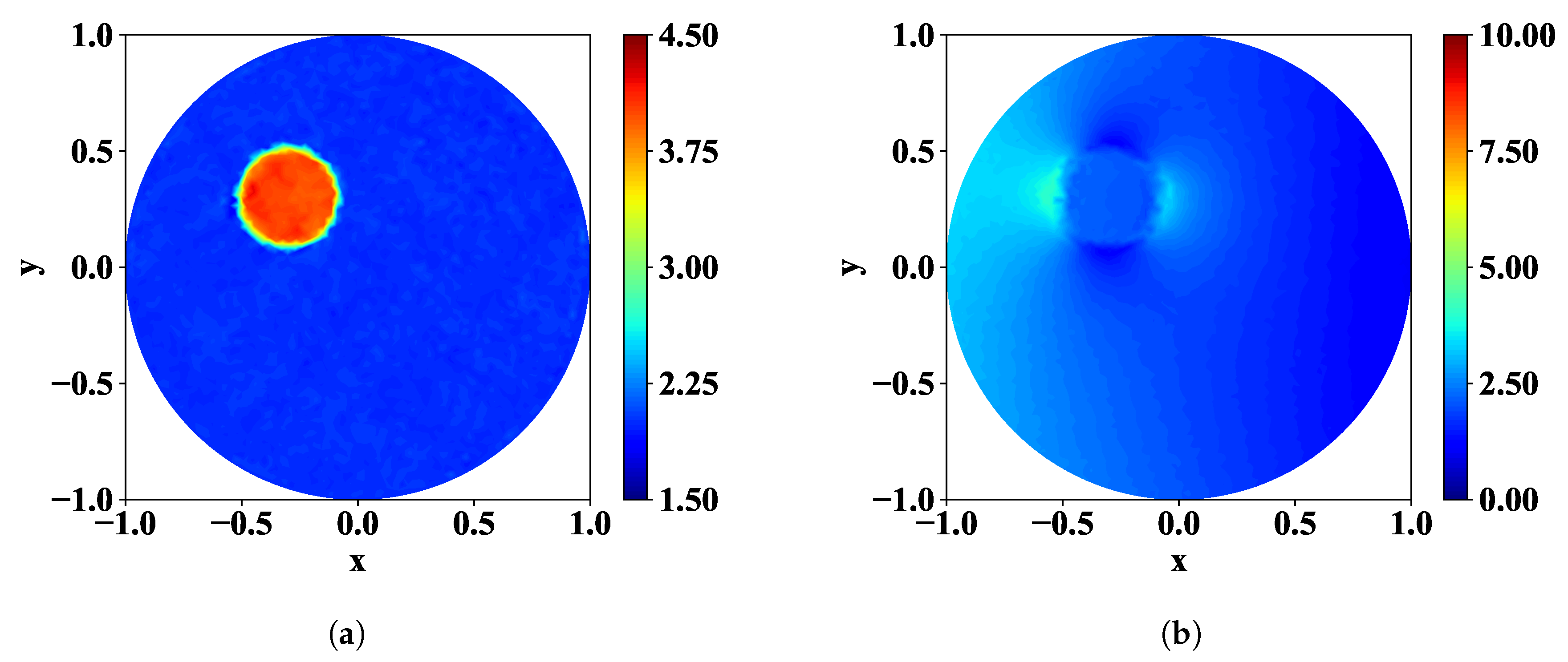
The minimum relative error $\eta =0.011$ is achieved at the 11th step when the conductivity of the interior circular domain is ${\sigma }_i=4.0 \mathrm{S}/\mathrm{m}$. The reconstructed conductivity distribution is shown in Figure 8a, and the corresponding power density is shown in Figure 8b. The reconstructed conductivity map is attractive although noise exists in the DOI, and the change of the power density across the boundary is not much. When the conductivity is further increased to ${\sigma }_i=12.0 \mathrm{S}/\mathrm{m}$, the computation starts to diverge after the 7th step, and the relative error begins to increase until to $\eta =0.142$. The reconstructed conductivity map and the power density of the 7th step are given in Figure 9a,b, and a larger change on the boundary of the interior domain is still observed, but the influence of the noise is not obvious.

However, when the noise level is further increased to SNR = 20 dB, the performance of the algorithm becomes more sensitive to the contrast. The variation of the relative errors corresponding to different conductivities is shown in Figure 10. The convergence of the computation is poor even for ${\sigma }_i=8 \mathrm{S}/\mathrm{m}$. For higher contrast, the computation converges well in the first several steps, but it starts to diverge afterwards. The minimum relative error $\eta =0.050 \mathrm{S}/\mathrm{m}$ is achieved at the 5th step when the conductivity of interior domain is $4.0 \mathrm{S}/\mathrm{m}$. The reconstructed conductivity map is shown in Figure 11a, and the corresponding power density is shown in Figure 11b. The results are obviously contaminated by noise, and fluctuation is observed in the DOI. This is caused by the large noise introduced into the power density as shown in Figure 11b.

To conclude, the performance of the introduced Levenberg–Marquardt method for acousto-electric tomography has a close relation with the contrast of the conductivity. It works adequately for a problem with low contrast and low noise level. This is observed when the contrast is smaller than 5. Then, the performance becomes worse with the increase of the contrast, and the minimum relative error also increases. However, higher noise will increase the sensitivity of the method to the contrast, and therefore decrease the stability of the algorithm and the quality of the reconstruction. These performances are also closely related to the smoothness of the distribution of power density in the domain of interest. However, it should not be neglected that the parameters ${\alpha }_k$ and ${\beta }_k$ introduced in (20) also play an important role.

3.3. Heart Lung Model

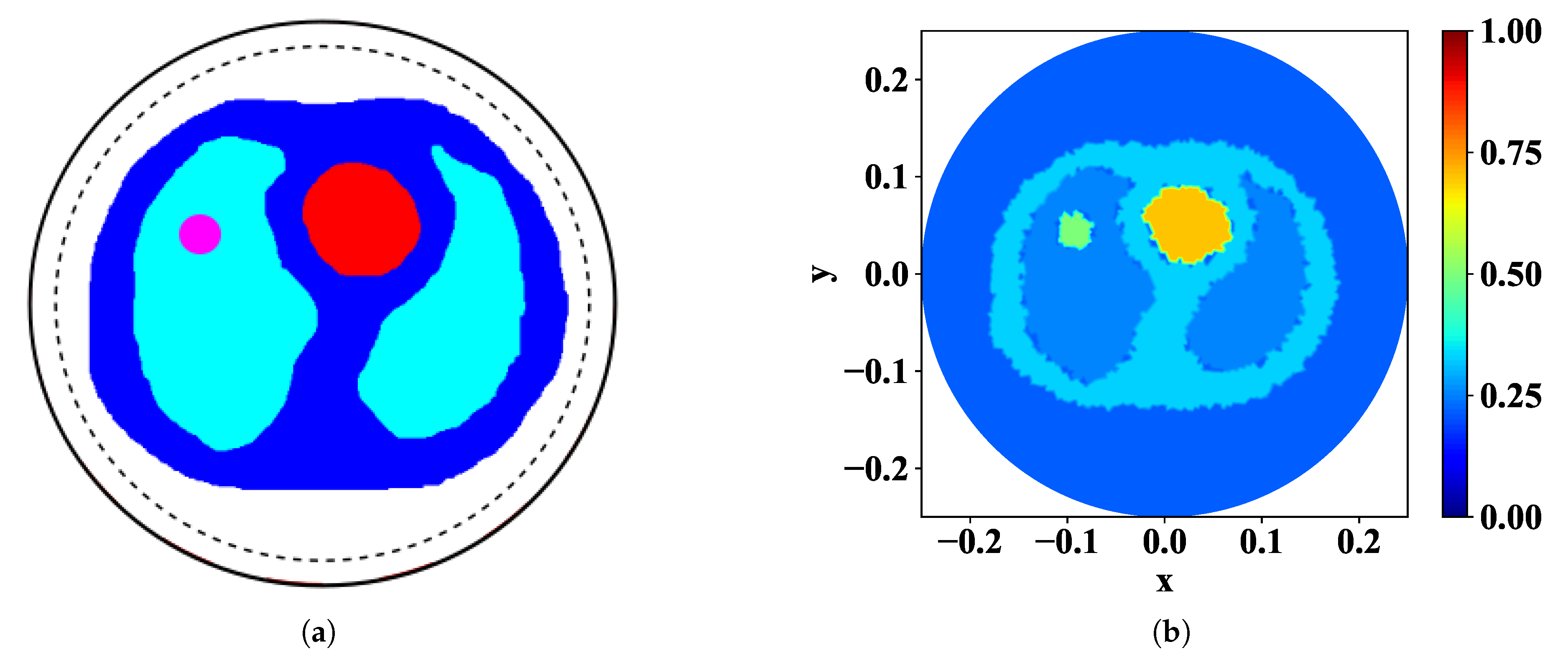
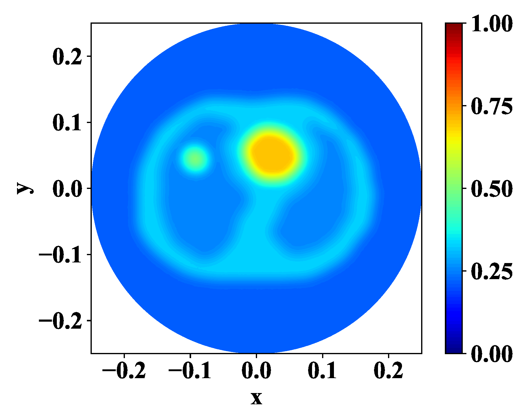
To further investigate the performance of the algorithm, a heart–lung model is created and used here, which is shown in Figure 12a. The considered tissues are heart (red, $\sigma$ = $0.7 \mathrm{S}/\mathrm{m}$), lung (cyan, $\sigma$ = $0.26 \mathrm{S}/\mathrm{m}$), and soft tissues (blue, $\sigma$ = $0.33 \mathrm{S}/\mathrm{m}$). Refer to the work in [16] for conductivities of different tissues. An additional circular domain is added to the left lung to simulate a lung cancer, and the tissue is in purple color. The conductivity of lung cancer tissue is generally 1.6 to 3.3 times larger than the normal tissues; here, it is set to $\sigma$ = $0.50\mathrm{S}/\mathrm{m}$, which is ~1.92 times of the lung tissue. The model is placed into a circular region with a background material $\sigma$ = $0.22 \mathrm{S}/\mathrm{m}$ and the radius is $0.25\mathrm{m}$. The true conductivity distributions are shown in Figure 12b. The inverse mesh consists of 12,539 vertices and 24,730 cells.The initial guess for the interaction is set to $0.22 \mathrm{S}/\mathrm{m}$ for the whole DOI. Here, ${\alpha }_k$ for the k-th iteration is set as ${\alpha }_k={\alpha }_0/a^k$ with ${\alpha }_0=1.0$, $a=2.0$, and ${\beta }_k$ is set as constant ${\beta }_0=1\times {10}^{-3}$.

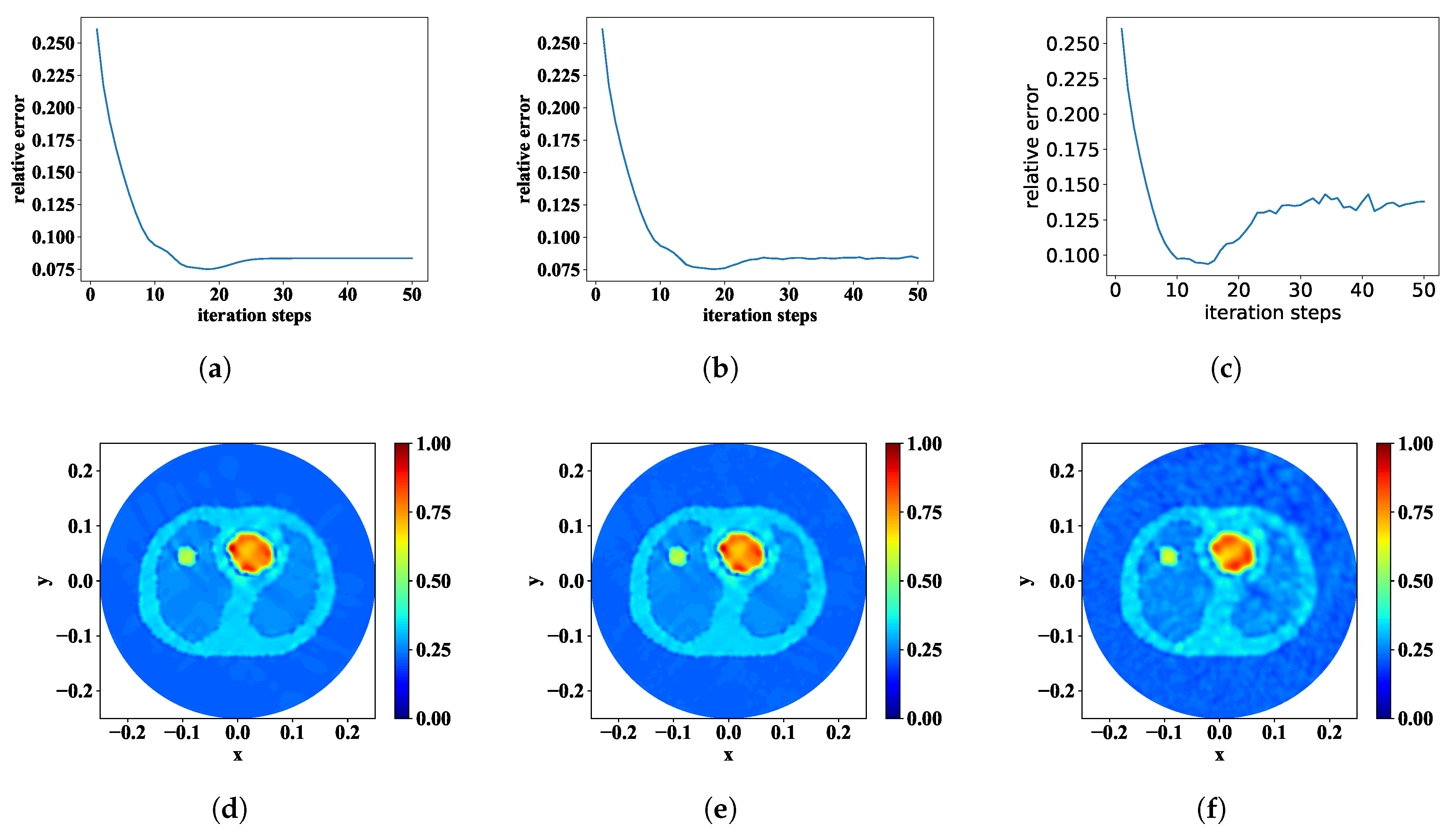
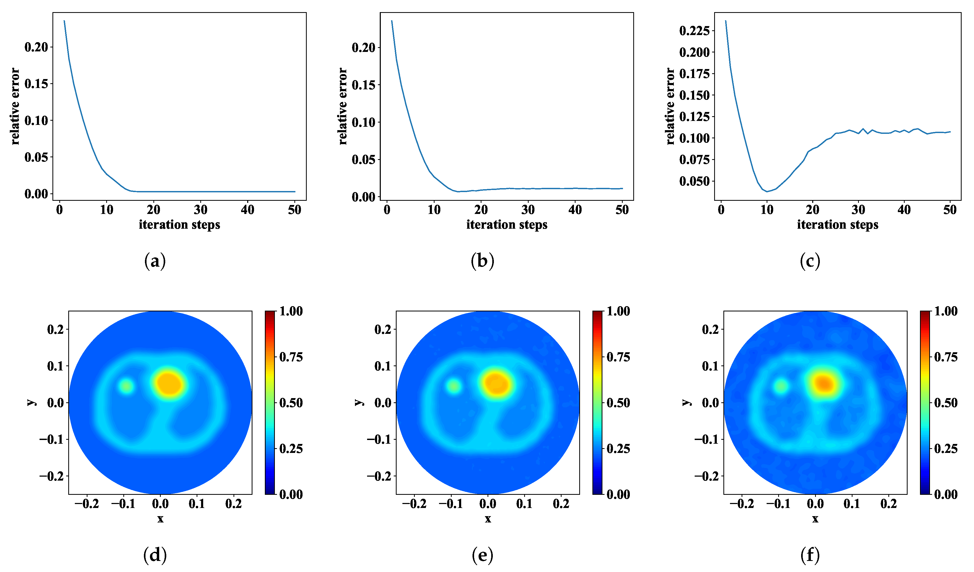
The conductivity is reconstructed with the method introduced in this paper. The relative error and reconstructed conductivity map with SNR = ∞, 40 dB, and 20 dB are shown in Figure 13a–c, respectively. In the computation, each iteration takes about 16 s and the total 50 iterations takes about 13 min. For the noise free case and the case with very low noise level as SNR = $40 \mathrm{dB}$, the minimum relative error is ~$0.074$. The convergence of the computation is fast, but the reconstructed results are not good, as can be seen in Figure 13a,b. When higher noise level is considered, the convergence of the computation becomes worse, and the reconstructed results are also not good. As seen in Figure 13c for SNR = $20 \mathrm{dB}$, although the general conductivity contribution is observed, and a minimum relative error $0.094$ is achieved, a lot of noise-like areas appear in the whole DOI. However, different tissues can still be clearly located in the reconstructed conductivity distribution, although their shapes are not so clear.

To investigate the influences of the conductivity jump on the boundaries of two subdomains in the DOI, a smooth–heart–lung model is obtained with a mollification operation. The piece-wised conductivity distribution is mollified with

$${\eta }_{ϵ}(x,y)=Cexp\left(\frac{{ϵ}^2}{(x^2+y^2)-{ϵ}^2}\right)$$

(23)

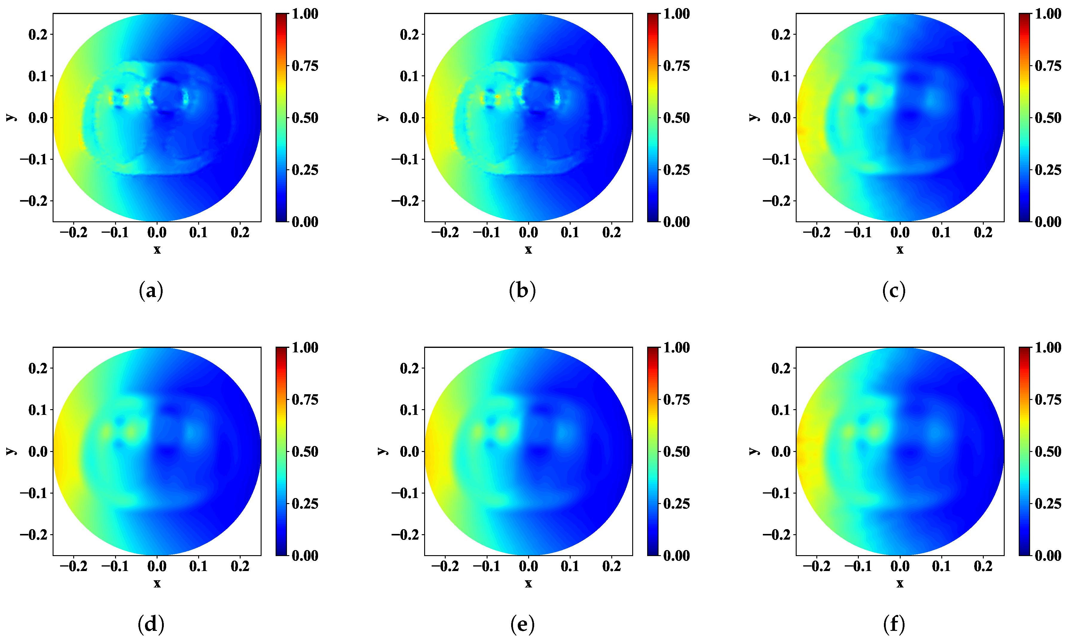
to produce $\sigma \in {\mathcal{H}}^s(\Omega )$ with $s=2$ for 2D problem. The constant $C>0$ is selected so that ${\int }_{R^2}{\eta }_{ϵ}=1$. The value of $ϵ$ is 1 cm for heart–lung model. The true smoothed distribution of $\sigma$ for the heart–lung model is shown in Figure 14. The numerical setup for the reconstruction of smoothed heart–lung model is kept. The relative error and reconstructed conductivity map of smooth–heart–lung model with SNR = ∞, 40 dB, 20 dB are shown in Figure 15. The minimum relative errors are ~$0.002$ when SNR = ∞ and $0.007$ when SNR = 40 dB, which is much smaller than the case with a piece-wised conductivity distribution. Even for the more noisy case with SNR = 20 dB, the minimum relative error is about $0.037$, which is also much smaller. The convergence of the computation also performs much better. This significant decrease of relative error and increase of convergence speed are mainly caused by the smoothness of the power density which is further resulted from the smoothed conductivity distribution. The power density of corresponding to the minimum relative errors for SNR = ∞, 40 dB, 20 dB are given in Figure 16 for both piece-wised and smoothed conductivity distributions of heart–lung model, respectively. A comparison shows that the power density for the smoothed conductivity is smoother, and there is no obvious discontinuity across the boundary of different subdomains. Therefore, a rather smooth distribution of the conductivity can lead to a smoothed power density distribution, and this can well improve the stability of the algorithm and accelerate the convergence as well.

4. Conclusions

The Levenberg–Marquardt method for the acousto-electric tomography is applied to reconstruct the conductivity distribution in the DOI from voltages measured on its boundary. The main focus has been on the influence of the contrast on the stability and convergence performance of the Levenberg–Marquardt method. It also discussed the influences of the regularization parameters. Several numerical investigations have been carried out for the illustration. The work herein, on the one hand, focuses on the higher contrast potential reconstruction method, and on the other hand, on validations of its practicability on detecting lung cancer.

It has been discovered that the algorithm becomes unstable when the contrast is approximately beyond 5. A contrast beyond this level will bring larger minimum relative error and a divergence after several iterations. The regularization parameter ${\alpha }_k$ plays an important role in the computation. A larger value of the ${\alpha }_k$ can make the computation converge better, but it will also render the convergence slower. A smaller ${\alpha }_k$ will bring a faster convergence as long as the solution is not too far from the true value, otherwise the algorithm will be unstable. Therefore, a strategy of decreasing ${\alpha }_k$ with the progress of the iteration can accelerate the convergence and keep the computation stable.

Theoretically, the conductivity distribution should be in the $H^2(\Omega )$ space, and the value of ${\beta }_k$ is closely related to the second order derivative of the conductivity distribution. When the contrast is too high, this continuity requirement can not be satisfied, a “V-shape” curve of the relative error appears. Therefore, the value of ${\beta }_k$ is also important for the stability and accuracy of the reconstruction. A large ${\beta }_k$ will enforce strong continuity requirement on the conductivity distribution, which will render the computation unstable. A small ${\beta }_k$ releases the continuity requirement, which will produce a poor reconstructed results. Therefore, the value of ${\beta }_k$ needs to be properly chosen. It is well known that the Tikhonov regularization can smooth the reconstructed conductivity, therefore a large ${\alpha }_k$ will balance the influence of a small ${\beta }_k$.

Besides the above parameters, a high contrast between the conductivity of different regions will cause a discontinuity of power density across the boundaries; this will not meet the continuity requirement in the reconstruction algorithm, which will also bring the instability and poor convergence, as demonstrated by the numerical results of the high noisy and high contrast cases.

The reconstructed results of a heart–lung model and a smooth–heart–lung model are compared to support the above conclusions, and a much better convergence and stability are observed with this smoothed heart–lung model.

However, it has been shown that the Levenberg–Marquardt method works quite well in general, and performs much better in low contrast case. The instability caused by the conductivity contrast can be improved with a proper Tikhonov regularization parameter. A simple dynamic strategy is used in this paper for choosing the proper value of Tikhonove regularization parameter ${\alpha }_k$, which requires the ground truth of the conductivity distribution. Although it works quite well in all the numerical results presented in the paper, it is not practical, as the ground truth is generally unknown in most cases. However, one can use the Morozov’s discrepancy principle for choosing this proper value, which should work better in theory.

References

- Martins, T.D.C.; Sato, A.K.; de Moura, F.S.; Camargo, E.D.L.B.d.; Silva, O.L.; Santos, T.B.R.; Zhao, Z.; Möeller, K.; Amato, M.B.P.; Mueller, J.L.; et al. A review of electrical impedance tomography in lung applications: Theory and algorithms for absolute images. Annu. Rev. Control. 2019, 48, 442–471. [Google Scholar] [CrossRef] [PubMed]
- Ammari, H.; Bonnetier, E.; Capdeboscq, Y.; Tanter, M.; Fink, M. Electrical impedance tomography by elastic deformation. SIAM J. Appl. Math. 2008, 68, 1557–1573. [Google Scholar] [CrossRef] [Green Version]
- Grasland-Mongrain, P.; Lafon, C. Review on biomedical techniques for imaging electrical impedance. IRBM 2018, 39, 243–250. [Google Scholar] [CrossRef]
- Roy, S.; Borzì, A. A new optimization approach to sparse reconstruction of log-conductivity in acousto-electric tomography. SIAM J. Imaging Sci. 2018, 11, 1759–1784. [Google Scholar] [CrossRef] [Green Version]
- Capdeboscq, Y.; Fehrenbach, J.; de Gournay, F.; Kavian, O. Imaging by modification: Numerical reconstruction of local conductivities from corresponding power density measurements. SIAM J. Imaging Sci. 2009, 2, 1003–1030. [Google Scholar] [CrossRef] [Green Version]
- Liu, S.; Jia, J.; Zhang, Y.D.; Yang, Y. Image reconstruction in electrical impedance tomography based on structure-aware sparse Bayesian learning. IEEE Trans. Med. Imaging 2018, 37, 2090–2102. [Google Scholar] [CrossRef] [Green Version]
- Liu, S.; Wu, H.; Huang, Y.; Yang, Y.; Jia, J. Accelerated structure-aware sparse Bayesian learning for three-dimensional electrical impedance tomography. IEEE Trans. Ind. Inform. 2019, 15, 5033–5041. [Google Scholar] [CrossRef]
- Dai, M.; Chen, X.; Chen, M.; Zeng, X.; Chen, S.; Sun, T.; Yu, L.; Hao, P.; Yan, J. A B-Scan imaging method of conductivity variation detection for magneto–acousto–electrical tomography. IEEE Access 2019, 7, 26881–26891. [Google Scholar] [CrossRef]
- Duan, X.; Koulountzios, P.; Soleimani, M. Dual modality EIT-UTT for water dominate three-phase material imaging. IEEE Access 2020, 8, 14523–14530. [Google Scholar] [CrossRef]
- Ammari, H.; Grasland-Mongrain, P.; Millien, P.; Seppecher, L.; Seo, J.-K. A mathematical and numerical framework for ultrasonically-induced Lorentz force electrical impedance tomography. J. Math. Pures Appl. 2015, 103, 1390–1409. [Google Scholar] [CrossRef]
- Hyvönen, N.; Mustonen, L. Smoothened complete electrode model. SIAM J. Appl. Math. 2017, 77, 2250–2271. [Google Scholar] [CrossRef] [Green Version]
- Hassan, H.; Semperlotti, F.; Wang, K.-W.; Tallman, T.N. Enhanced imaging of piezoresistive nanocomposites through the incorporation of nonlocal conductivity changes in electrical impedance tomography. J. Intell. Mater. Syst. Struct. 2018, 29, 1850–1861. [Google Scholar] [CrossRef]
- Zhao, L.; Yang, J.; Wang, K.; Semperlotti, F. An application of impediography to the high sensitivity and high resolution identification of structural damage. Smart Mater. Struct. 2015, 24, 065044. [Google Scholar] [CrossRef] [Green Version]
- Hubmer, S.; Knudsen, K.; Li, C.Y.; Sherina, E. Limited-angle acousto-electrical tomography. Inverse Probl. Sci. Eng. 2018, 27, 1298–1317. [Google Scholar] [CrossRef] [Green Version]
- Adesokan, B.J.; Jensen, B.; Jin, B.; Knudsen, K. Acousto-electric tomography with total variation regularization. Inverse Probl. 2019, 35, 035008. [Google Scholar] [CrossRef] [Green Version]
- Li, C.Y.; Karamehmedovic, M.; Sherinac, E.; Knudsen, K. Levenberg–Marquardt algorithm for acousto-electric tomography based on the complete electrode model. arXiv 2019, arXiv:1912.08085. [Google Scholar]
- Bal, G.; Naetar, W.; Scherzer, O.; Schotland, J. The Levenberg–Marquardt iteration for numerical inversion of the power density operator. J. Inverse Ill Posed Probl. 2013, 21, 265–280. [Google Scholar] [CrossRef] [Green Version]
- Jossinet, J.; Lavandier, B.; Cathignol, D. Impedance modulation by pulsed ultrasound. Ann. N. Y. Acad. Sci. 1999, 873, 396–407. [Google Scholar] [CrossRef]
- Somersalo, E.; Cheney, M.; Isaacson, D. Existence and uniqueness for electrode models for electric current computed tomography. SIAM J. Appl. Math. 1992, 52, 1023–1040. [Google Scholar] [CrossRef]
- Jossinet, J.; Trillaud, C.; Chesnais, S. Impedance changes in liver tissue exposed in vitro to high-energy ultrasound. Physiol. Meas. 2005, 26, S49–S58. [Google Scholar] [CrossRef]
- Kuchment, P. Mathematics of hybrid imaging: A brief review. In The Mathematical Legacy of Leon Ehrenpreis; Springer: Milano, Italy, 2012; pp. 183–208. [Google Scholar]
- Song, X.; Xu, Y.; Dong, F. Linearized image reconstruction method for ultrasound modulated electrical impedance tomography based on power density distribution. Meas. Sci. Technol. 2017, 28, 045404. [Google Scholar] [CrossRef]
- Adams, R.A. Sobolev Spaces; Academic Press: New York, NY, USA, 1975. [Google Scholar]
- Kaltenbacher, B.; Neubauer, A.; Scherzer, O. Iterative Regularization Methods for Nonlinear Ill-Posed Problems; De Gruyter: Berlin, Germany, 2008. [Google Scholar]
- Moré, J.J. The Levenberg–Marquardt algorithm: Implementation and theory. In Numerical Analysis: Proceedings of the Biennial Conference Held at Dundee; Springer: Berlin/Heidelberg, Germany, 1978; pp. 105–116. [Google Scholar]
- Lechleiter, A.; Rieder, A. Newton regularizations for impedance tomography: Convergence by local injectivity. Inverse Probl. 2008, 24, 065009. [Google Scholar] [CrossRef]
- Newton regularizations for impedance tomography: A numerical study. Inverse Probl. 2006, 22, 1967–1987. [CrossRef]
- Brusset, H.; Depeyre, D.; Petit, J.-P.; Haffner, F. On the convergence of standard and damped least squares methods. J. Comput. Phys. 1976, 22, 534–542. [Google Scholar] [CrossRef]
- Hanke, M. A regularizing Levenberg–Marquardt scheme, with applications to inverse groundwater filtration problems. Inverse Probl. 1997, 13, 79. [Google Scholar] [CrossRef]
- Kreyszig, E. Introductory Functional Analysis with Applications; John Wiley & Sons: New York, NY, USA, 1978. [Google Scholar]
- Langtangen, H.P.; Logg, A. Solving PDEs in Hours—The FEniCS Tutorial Volume II; Springer: New York, NY, USA, 2016. [Google Scholar]
Figure 1.
The mesh used in numerical examples: (a) the mesh of forward model and (b) the mesh of inverse problem.
Figure 2.
The variation of relative error of different with various conductivities: (a) when SNR = 40 dB and (b) when SNR = 20 dB.
Figure 3.
The relative error of different with different conductivities: (a) when SNR = 40 dB and (b) when SNR = 20 dB.
Figure 4.
The relative error of each conductivity when SNR = ∞.
Figure 5.
When SNR = ∞, and the step is 12: (a) the reconstructed image and (b) the power density.
Figure 6.
When SNR = ∞, and the step is 7: (a) the reconstructed image and (b) the power density.
Figure 7.
The relative error of each conductivity when SNR = 40 dB.
Figure 8.
When SNR = 40 dB, and the step is 11: (a) the reconstructed image and (b) the power density.
Figure 9.
When SNR = 40 dB, and the step is 7: (a) the reconstructed image and (b) the power density.
Figure 10.
The relative error of each conductivity when SNR = 20 dB.
Figure 11.
When SNR = 20 dB, and the step is 5: (a) the reconstructed image and (b) the power density.
Figure 12.
The heart–lung model: (a) the region of different organs and (b) true conductivity distributions.
Figure 13.
The variation of the relative error for (a) SNR = ∞, (b) SNR = 40 dB, and (c) SNR = 20 dB. The reconstructed conductivity distribution for (d) SNR = ∞, (e) SNR = 40 dB, (f) SNR = 20 dB.
Figure 14.
The true conductivity distributions of smooth–heart–lung model.
Figure 15.
The relative error and reconstructed conductivity map of smooth-heart–lung model with (a,d) for SNR = ∞, (b,e) for SNR = 40 dB, (c,f) for SNR = 20 dB.
Figure 16.
The power density corresponding to heart–lung model (top row) and smooth–heart–lung model (bottom row) at the iteration step where the minimum relative error achieved. (a,d) for SNR = ∞, (b,e) for SNR = 40 dB, (c,f) for SNR = 20 dB.
© 2020 by the authors. Licensee MDPI, Basel, Switzerland. This article is an open access article distributed under the terms and conditions of the Creative Commons Attribution (CC BY) license (http://creativecommons.org/licenses/by/4.0/).
Share and Cite
MDPI and ACS Style
Li, C.; An, K.; Zheng, K. The Levenberg–Marquardt Method for Acousto-Electric Tomography on Different Conductivity Contrast. Appl. Sci. 2020, 10, 3482. https://doi.org/10.3390/app10103482
AMA Style
Li C, An K, Zheng K. The Levenberg–Marquardt Method for Acousto-Electric Tomography on Different Conductivity Contrast. Applied Sciences. 2020; 10(10):3482. https://doi.org/10.3390/app10103482
Chicago/Turabian StyleLi, Changyou, Kang An, and Kuisong Zheng. 2020. "The Levenberg–Marquardt Method for Acousto-Electric Tomography on Different Conductivity Contrast" Applied Sciences 10, no. 10: 3482. https://doi.org/10.3390/app10103482
Note that from the first issue of 2016, this journal uses article numbers instead of page numbers. See further details here.