Limitations of Boulder Detection in Shallow Water Habitats Using High-Resolution Sidescan Sonar Images


1
Institute of Geosciences, Coastal Geology and Sedimentology, Kiel University, 24118 Kiel, Germany
2
State Agency for Agriculture, Environment and Rural Areas (LLUR), 24220 Flintbek, Germany
*
Author to whom correspondence should be addressed.
Geosciences 2019, 9(9), 390; https://doi.org/10.3390/geosciences9090390
Submission received: 30 July 2019
/
Revised: 30 August 2019
/
Accepted: 4 September 2019
/
Published: 6 September 2019
(This article belongs to the Special Issue Geological Seafloor Mapping)
Abstract
:Stones and boulders in shallow waters (0–10 m water depth) form complex geo-habitats, serving as a hardground for many benthic species, and are important contributors to coastal biodiversity and high benthic production. This study focuses on limitations in stone and boulder detection using high-resolution sidescan sonar images in shallow water environments of the southwestern Baltic Sea. Observations were carried out using sidescan sonars operating with frequencies from 450 kHz up to 1 MHz to identify individual stones and boulders within different levels of resolution. In addition, sidescan sonar images were generated using varying survey directions for an assessment of range effects. The comparison of images of different resolutions reveals considerable discrepancies in the numbers of detectable stones and boulders, and in their distribution patterns. Results on the detection of individual stones and boulders at approximately 0.04 m/pixel resolution were compared to common discretizations: it was shown that image resolutions of 0.2 m/pixel may underestimate available hard-ground settlement space by up to 42%. If methodological constraints are known and considered, detailed information about individual stones and boulders, and potential settlement space for marine organisms, can be derived.
1. Introduction
Stones and boulders in shallow waters form important geo-habitats in which many species coexist. Consequently, they are important contributors to coastal biodiversity and high benthic production. These habitats provide valuable feeding areas, and spawning and nursing grounds for fish [1,2,3]. Human impact on coastal habitats is increasing and benthic communities living in these environments are particularly affected [4,5,6,7]. Hard-bottom substrates occurring in the Baltic Sea are generally stones (θ 6.3–20 cm) and boulders (θ 20–630 cm) [8]. The need for mapping and understanding small-scale seabed features like stone and boulder assemblages, combined with habitat assessment, is growing significantly, as European legislations and directives are demanding the documentation and monitoring of environmental states [9]. Due to their valuable characteristics, hard-bottom substrates (e.g., stones and boulders) are protected in the Baltic Sea by the European Habitats Directive (HD 92/43/EEC annex 1 1170–reefs) [10].
From about, 1800–1976, stones and boulders were commercially extracted from shallow submarine areas of the southwestern Baltic Sea [11]. These “stone fishing” activities have changed the sedimentological structure and ecological conditions of the coastal waters, as stones and boulders form an important environment for marine organisms [12]. Approximately 3.5 × 10⁶ tons of boulders ranging from 60 to 150 cm in diameter have been extracted, equivalent to a surface area of hard bottom substrate of about 5.6 km2 [11]. However, there are still boulders present despite the previous removal, and their number is increasing over the course of decades due to abrasion processes exposing new stones and boulders from glacial till forming the seafloor [13].
The difference in spatial scale between individual stones and the large extents of boulder assemblages, their spatial heterogeneity and their temporal development require remote sensing observation techniques. Whereas airborne techniques and satellite remote sensing may be limited by resolution, vegetation and water turbidity, ship based hydro-acoustic techniques, such as sidescan sonar (SSS hereafter) or multibeam echosounder (MBES), allow the investigation of the seafloor in high-resolution and at turbid water conditions [14,15,16,17,18]. In coastal waters of the Baltic Sea, a great variety of sediment types and geomorphological features characterize the seafloor. Many shallow water seafloor features are only visible at high-resolution, thus require the use of higher acoustic frequencies [14]. SSSs with high frequencies allow the generation of high-resolution images but also inherit acoustic challenges. Due to absorption loss, higher frequencies are not able to propagate very far and the operating range decreases, resulting in more time consuming surveys [14,15,19].
Many surveys have been carried out to localize ecologically important marine habitats (>10 m water depth) using SSS [13,16,18,20] and have successfully demonstrated the suitability of SSS to map and identify areas with stone and boulder occurrence. Various authors used a wide range of instruments, with different characteristics and survey settings, resulting in quantitative assessments of habitats [16,21,22,23,24,25]. The identification of objects using multibeam echo sounders (MBES) has been shown for, e.g., mine detection [20,26]. Area-wide habitat mapping is often performed by using acoustic frequencies ranging from 300 to 500 kHz, survey speeds vary between 2–4 m/s and across-track ranges between 50 m and 180 m [13,16,18,27]. Those survey setups generate SSS image resolutions ranging from 0.25 m/pixel to 1 m/pixel, thus are insufficient to identify individual stones or boulders, especially in areas with coarse, mixed sediments [16]. Despite recent advances in methods for the automated detection of individual stones and boulders [27,28] methodological constraints of survey settings (acoustic frequencies, horizontal resolution and range, survey speeds, etc.) remain undiscussed.
In this study, we show the limitations using high-resolution SSS data to identify individual stones and boulders in shallow water, in order to contribute to the discussion on:
- (a)
- What SSS image resolution is required to quantify stones and boulders in shallow water areas?
- (b)
- How do range settings influence the detection quality of individual stones and boulders in high-resolution SSS images?
Regional Setting
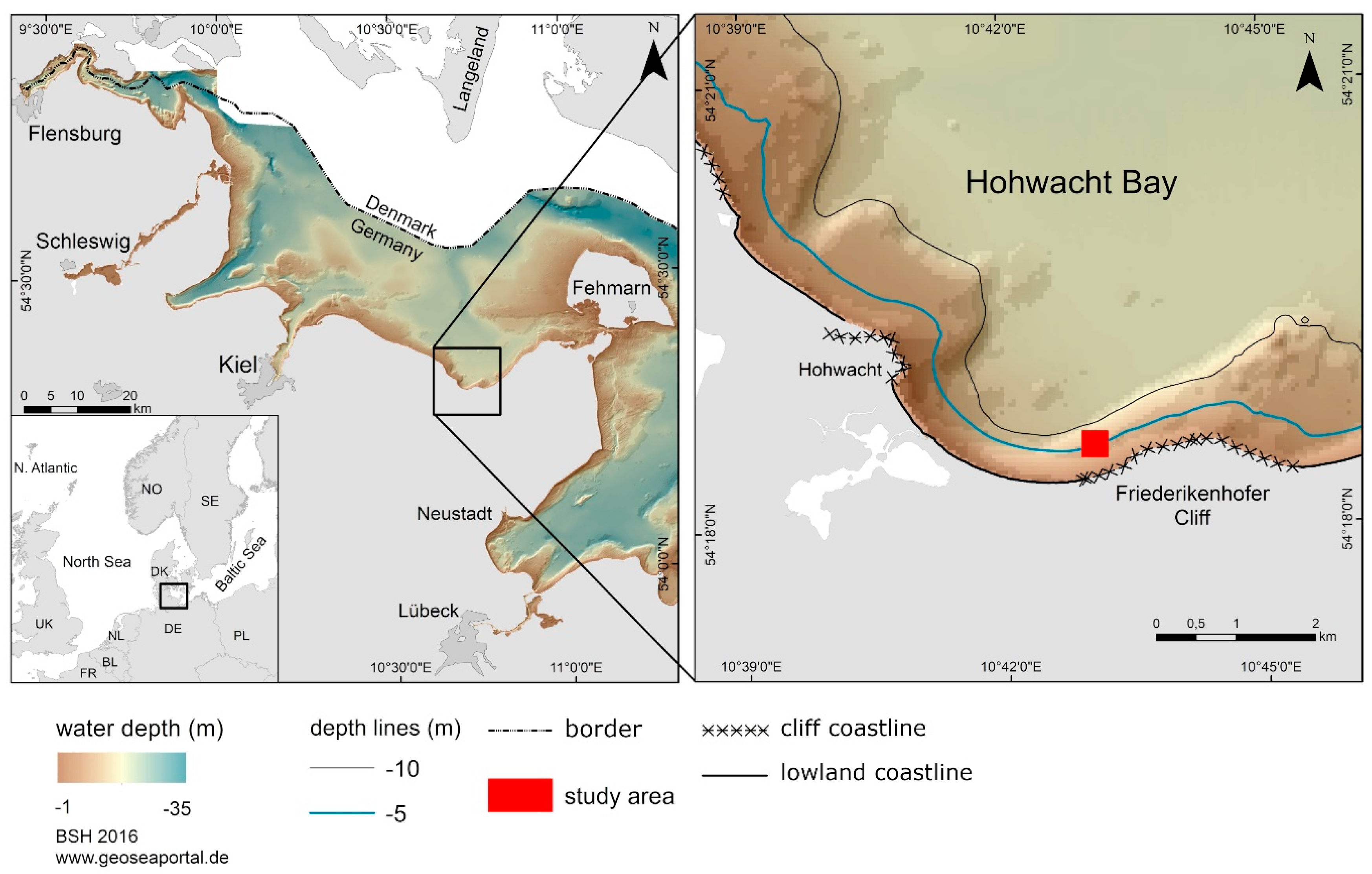
The seabed of Hohwacht Bay, located in the southwestern Baltic Sea (Figure 1), is mainly built of glacial till deposits with grain sizes ranging from clay to boulders [29]. Stones and boulders are distributed randomly within these deposits [13]. The evolution of the Baltic Sea is characterized by postglacial sea level fluctuations. The Littorina transgression started at about 8000 years BP and ceased at about 5000 years BP [30,31]. That sea level rise flooded the postglacial landscape. During phases of slower rising or even stagnation of water levels, erosion supported the evolution of abrasion platforms [32]. Those are common features in the southwestern Baltic Sea, especially in front of active cliffs [32,33,34]. As these shallow water environments (0–10 m depth) are strongly influenced by waves and currents, the platforms are abrading, with fine material being eroded and transported offshore and alongshore, while coarser material like stones and boulders are left behind on the platform. Thus, the sedimentological composition of the shallow water Baltic seafloor is of high spatial and temporal heterogeneity.
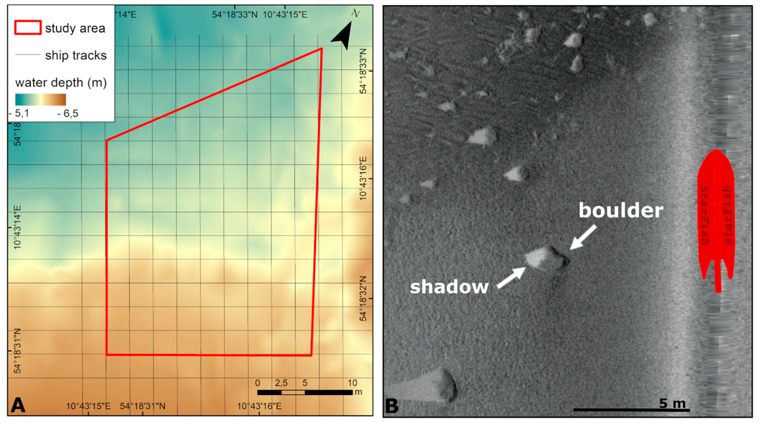
This study is based on hydro-acoustic data of a small observation area with a size of approximately 25 × 25 m, within the inner Hohwacht Bay. It is located 300 m offshore of the Friederikenhofer Cliff (Figure 1). Water depths range from 5.50 to 6.30 m and the investigation site is exposed to wind and waves from the northwest via north to northeast.
2. Methods
High-resolution seafloor mapping techniques with SSS are frequently used to investigate the seafloor in coastal waters. However, most of these surveys are carried out in areas of >10 m water depth. To assess the applicability of SSS for the investigation of individual stones and boulders in very shallow waters, we deployed different small-scale SSSs (StarFish 452F and StarFish 990F (Tritech)) to a small rubber boat. They were deployed to detect, measure and compare individual stones and boulders and their spatial distribution. To exclude distortions by boat movement or noise due to bad weather conditions, which may affect the quality of SSS images, a day with ideal survey conditions was selected for measurements, containing very low wind speeds of 2 m/s from the southeastern direction, and no waves. Therefore, influences of pitch, roll, yaw and heave do not need to be considered for this dataset.
The StarFish SSS uses a compressed high-intensity radiated pulse (chirp) transmission as the frequency changes through the duration of the transmission (e.g., StarFish 452 F operates between 430 kHz and 470 kHz). Two transducers operate in separate channels for port and starboard sidescan intensities (Table 1). The two SSS devices were applied to generate images with resolutions ranging from 0.2 m/pixel to 0.04 m/pixel. In addition, measurements were executed from the four borders of the study area. The surveys were executed with varying headings and survey speeds to compare resolution and range impacts from the four different sides of the study area (Table 1, Figure 2).
We classified the SSS images into three levels: low, medium and high resolution (Table 1). The low-resolution SSS image was generated with a range of 50 m, a survey speed of 2.3 m/s and a frequency of 450 kHz to achieve a resolution of 0.2 m/pixel (Table 1). One low-resolution SSS image measured along the southeastern border was used for resolution and range analysis. The medium-resolution was generated with a range of 35 m, 1.0 m/s survey speed and a frequency of 1 MHz, to create SSS images with a resolution of 0.1 m/pixel (Table 1). Four SSS images were generated from the outer edges of the study area (Figure 2, red lines) for resolution and range analysis. The high-resolution SSS images were generated with a range of 10 m, a survey speed of 1.0 m/s and a frequency of 1 MHz, achieving a resolution of 0.04 m/pixel (Table 1). Ship tracks crossing the study area are spaced at 2.5 m increments to generate SSS images with the highest resolution. To obtain the highest resolution of 0.04 m/pixel, and therefore the best image data quality, we selected high quality mid-range sections of five SSS images. These sections were merged to cover the study area (Table 1). It is noted that, compared to SSS image resolutions commonly used to detect stone and boulder assemblages; the resolution of 0.2 m/pixel (low resolution), is still relatively high. For accurate positioning, we used a DGPS (GNSS 1200+; Leica) with RTK accuracy, combined with a heading sensor (Garmin Airmar). A single-beam echo sounder with an integrated DGPS was utilized to map the water depth within the study area.
Post-processing of the SSS images involved standard geometric and radiometric corrections [14,15] done with the software SonarWiz 7.03 (Chesapeake Technology Inc.) [36]. In order to correct for transmission losses, a time varying gain (TVG) was applied after slant-range correction to all datasets. Areas with high backscatter intensities are displayed in darker grey-levels than low backscatter areas. Detailed explanation about the SSS technique is given in the literature [14,15,37,38,39]. Stones and boulders, like any three-dimensional objects, can be detected by local high backscatter intensities (dark areas) combined with their characteristic (bright) shadow [14,15,37] (Figure 2). All stones and boulders were counted manually in the waterfall mode of SonarWiz. ArcMap 10.6 (Esri) was used for gridding and map creation.
The scientific diving group of Kiel University did a ground-truthing within the study area. This included underwater video observations and sediment sampling to generate a sediment distribution map. Grain size distributions of sediment samples were obtained by mechanical sieving, using ¼ PHI intervals according to the ASTM mesh standard. Statistical parameters from the grain size distribution were gained using the software GRADISTAT [40]. Grainsize classification was executed using the Kolp classification scheme (e.g., fine sand (0.1–0.2 mm), medium sand (0.2–0.63 mm), stones (6.3–20 cm) and boulders (20–630 cm)) [8]. Stones and boulders will not explicitly be differentiated by their size; hereafter both will be named “boulders.”
High, medium and low-resolution SSS images measured from the southeastern border of the study area were used to analyze how the SSS image resolution affects the detection quality of individual stones and boulders. Detected numbers of boulders are compared from each SSS image. Boulder counts derived from medium and high-resolution SSS images (from the four borders) are each subdivided in one-meter steps along the range. These subdivided boulder counts are displayed in dependency to their occurring distance to the transducer to identify the range settings influence on the detection quality of individual stones and boulders.
Boulder surface calculations are used to assess the approximate amount of settlement space within the study area. For simplicity, a calculation of hemisphere surfaces for the detected boulders in each level of SSS image resolution was done. The number of detected boulders was derived from manual counting of features within the SSS images. The approximate diameter of the identified boulders was estimated using the minimum detection size for each level of resolution. For the low resolution (0.2 m/pixel), that is a value of 0.4 m. The minimum detection diameter for the medium resolution (0.1 m/pixel) is 0.2 m and for the high resolution (0.04 m/pixel) 0.08 m. The boulder counts of each SSS image were subdivided using the minimum detection size as a proxy for the diameter. For example, the boulder count derived from the high-resolution SSS image is divided into the three minimum detection sizes. The calculated surface area indicates an estimation of the “potential settlement space” for marine organisms to settle on.
3. Results
3.1. Study Area
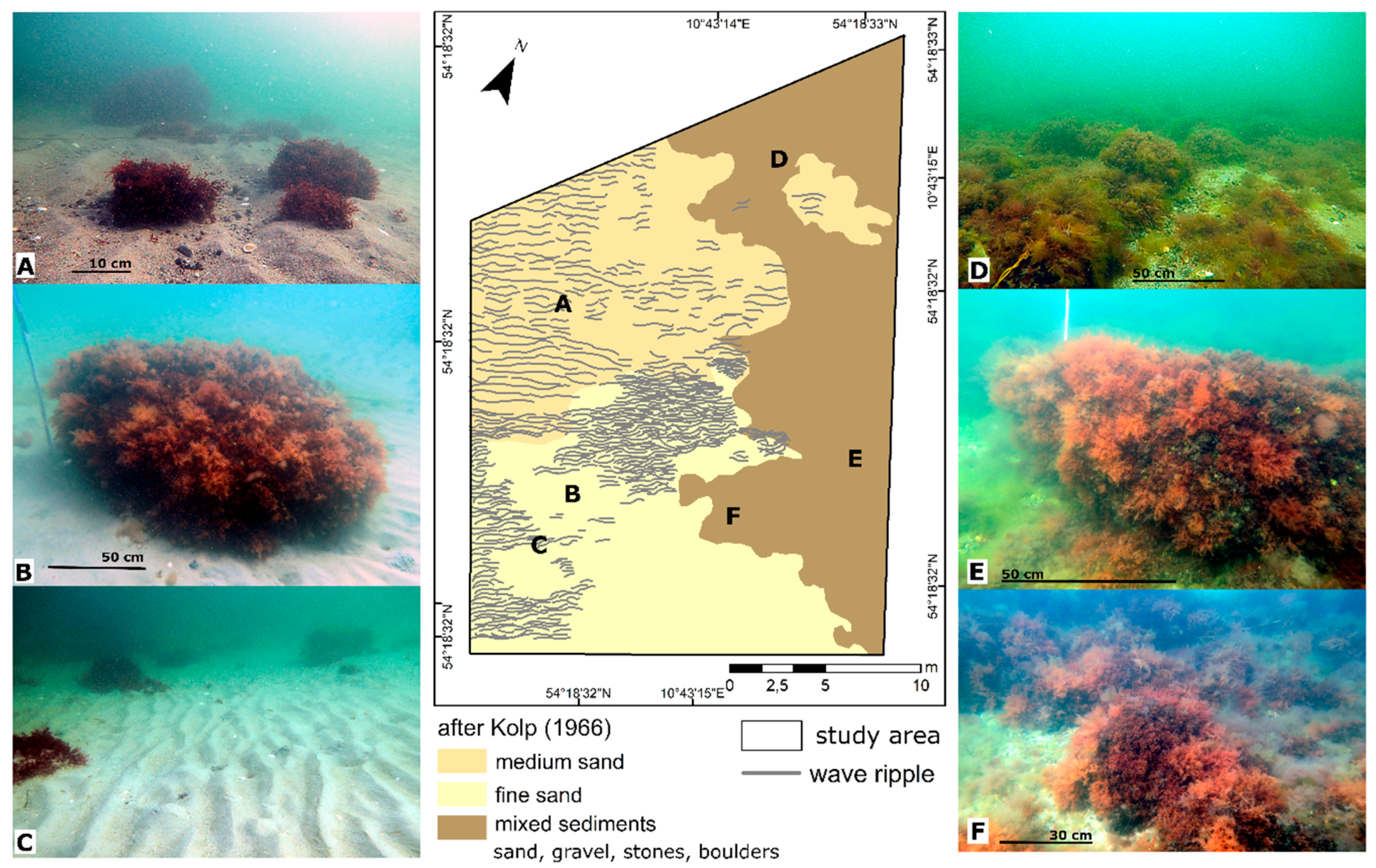
The observed area covers approximately 625 m2. The backscatter mosaic of the study area combined with the ground truthing and sediment analysis indicates two sedimentological zones. The southern zone is dominated by sandy sediment (fine to medium sands (Ø 0.1–0.63 mm)) (Figure 3). Wave ripples are frequently observed within these areas, particularly in its southwestern part (Figure 3A–C). Gravel and shells appear within the ripple valleys (Figure 3A). Isolated boulders or small boulder assemblages are observed within the sandy sediment (Figure 3A–C). In contrast, mixed sediment characterizes the northern zone, where grainsizes range from sand to gravel (Figure 3D,E). Stones and boulders occur throughout the complete northern zone in higher numbers than in the southern zone (Figure 3D–F). Stones and boulders within the whole study area are typically vegetated (e.g., algae, sponges). The study area shows a seaward sloping relief. Water depth in the study area ranges from 5.50 m in the southern part to 6.30 m in the northern part (Figure 3).
3.2. Effect of Resolution
All SSS images of different resolution can be used to distinguish between single boulders and the surrounding sediment matrix. However, comparing SSS images with different resolutions revealed considerable discrepancies in individual boulder detection and distribution patterns (Figure 4A–C).
In the low-resolution SSS image, 109 individual boulders were identified (Figure 4A). The southern zone is characterized by medium backscatter intensities and contains the highest amount of boulders. The northern part of the study area displays the highest backscatter. Disturbances are observed in the northeastern part of the SSS image and make boulder detection almost impossible in this region (Figure 4A, Table 2).
Figure 4B shows the medium resolution SSS image, where in total 384 boulders were identified. Again, the southern zone displays medium backscatter intensities and the highest boulder count is found in the east of this zone. A homogeneous and blurry area, indicating a lack of data points or image distortion, dominates the northern zone of this medium-resolution SSS image. Therefore, identification of boulders or other seafloor features is difficult (Figure 4B, Table 2).
The highest resolution SSS image results from a merged dataset and is considered closest to the true state (Figure 4C). Again, homogeneous medium backscatter intensities dominate the southern area. The highest number of boulders is also found on the eastern side of this zone. In contrast to the low and medium-resolution image, here the northern zone displays high backscatter intensities with wave ripples in the northwest, and the highest boulder accumulations in the northeastern area (Figure 4C, Table 2). The different settings result in different boulder counts. At a resolution of 0.2 m/pixel, which compares well to common habitat mapping resolutions, 83% less boulders are identified compared to the highest resolution image (Table 1).
Figure 4D displays the number of boulders detected in dependency of the SSS range. Compared to the high resolution, the medium resolution image displays similar minima and maxima of boulder counts up to a range of 12 to 15 m. Between 12 and 20 m, the medium resolution also depicts peaks, but the number of boulders decreases by 60%. From a distance of 20 m from the southeastern border, boulder counts decrease to zero, whereas the data of the high-resolution still depicts boulders. When considering the low-resolution image, a peak at around 10 m from the southeastern border can still be identified; however, the total count of boulders is far less (Figure 4D).
Surface estimations were done for the boulders identified at each resolution level. The approximate diameters of the boulders were estimated using the minimum detection sizes (Table 2). To simplify the boulder surface calculations, all boulders are assumed hemispheres. Comparing these potential settlement spaces, differences are observable between the images with different resolutions (Table 3). The image with the low resolution reveals 109 boulders with a minimum diameter of 0.4 m, resulting in a potential settlement space of 41 m2. The image with the medium resolution includes 384 boulders, 109 with a diameter of 0.4 m and 275 boulders with a diameter of 0.2 m. Thus, a potential settlement space of 67 m2 is calculated. 649 boulders are identified within the high-resolution SSS image, of which the surface is calculated: 109 boulders were present with diameters of 0.4 m, 275 boulders had a diameter of 0.2 m and 265 boulders had a diameter of 0.08 m. A total potential settlement space of 71 m2 was calculated. Compared to the high-resolution image, the low-resolution image indicates only 58% of settlement space provided by all identified boulders.
3.3. Effect of the Range
The dependency of the detection quality on range settings was further explored by SSS images generated from different sides of the survey area (Figure 5 and Figure 6). Counting individual boulders from different images resulted in differences in counts and distribution patterns (Figure 5). At appropriate angles, wave ripples are detected (Figure 5 and Figure 6). SSS images of the study site reveal a range effect, as dissimilar numbers of boulders within the same level of resolution are detected.
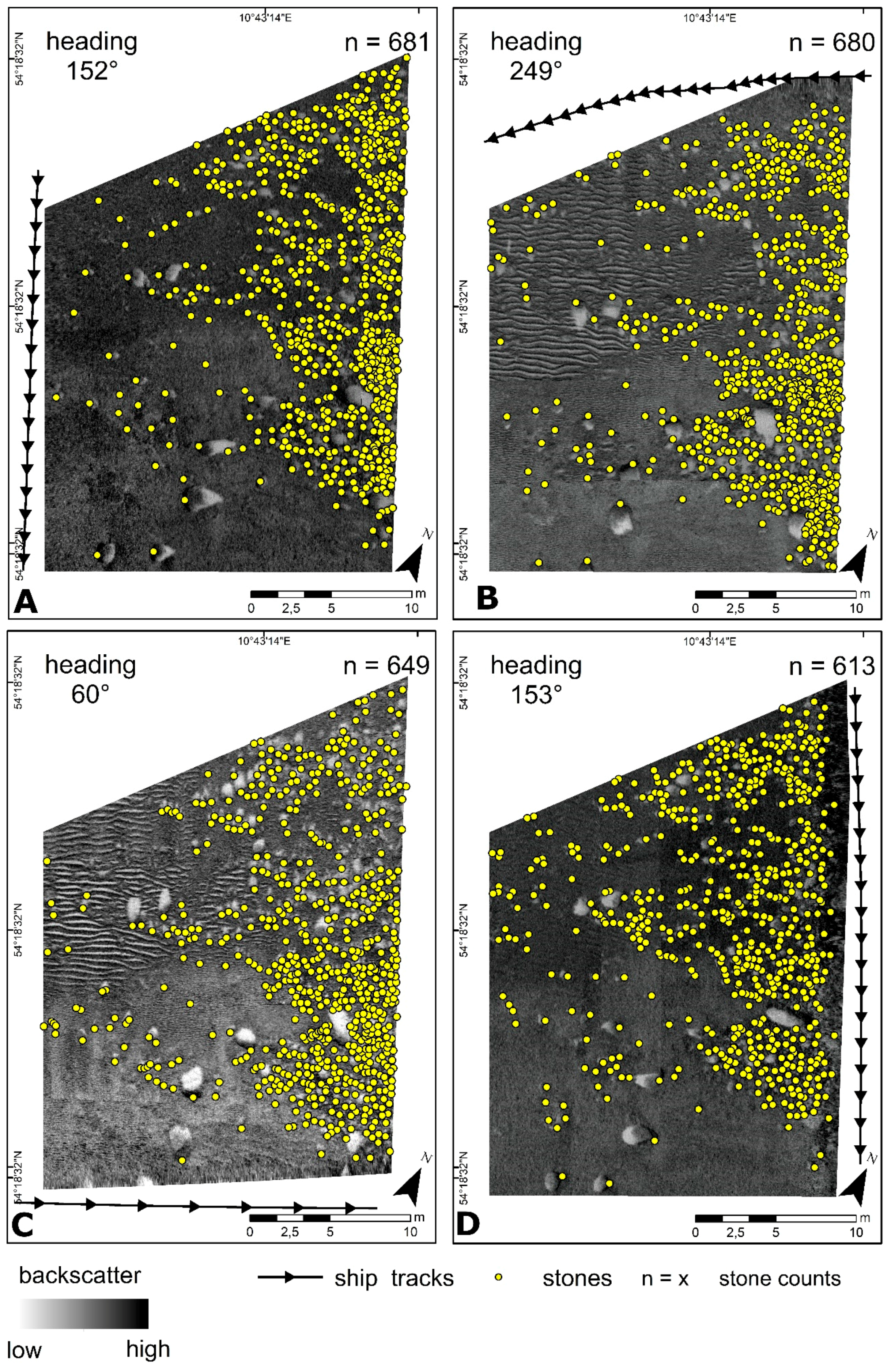
Comparing medium resolution SSS images generated from the four different sides of the study area, numbers of detected boulders range from 339 to 540 for the study area—a difference of 37%. The outer areas of the SSS images display a diffuse backscatter where the detection of boulders is difficult or impossible (Figure 5). A range dependency is observable in all images, regardless of the approach position. In order to determine whether the discrepancies in boulder counting decrease with higher resolution, we compared SSS images from the four outer edges on high-resolution data sets (Figure 6). A minimum boulder count of 613 and a maximum of 681 was found—a divergence of 10%.
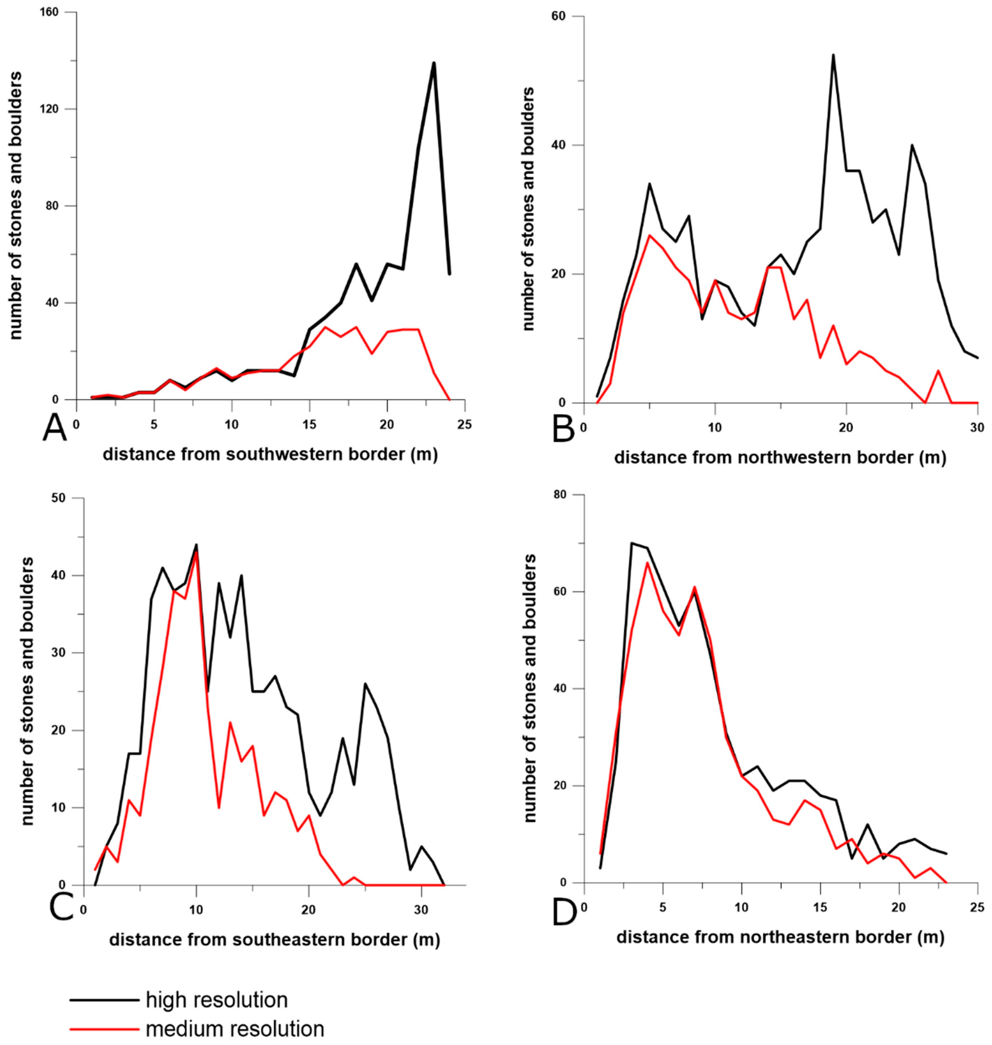
We plotted the abundance of boulders of both resolutions in relation to distance to the transducer (Figure 7A–D). The boulder distribution extracted from the high-resolution SSS images reveal a number of peaks along the whole range. Comparing numbers of boulders collected from the medium-resolution SSS images, a similar distribution pattern was observed up to mid-range distances of 10–15 m (Figure 7A–D). Then, a strong reduction in the medium-resolution boulder count with increasing range occurs, regardless of the approach position. Peaks in high-resolution numbers of boulders are significantly smaller or non-existent in medium-resolution boulder counts, with differences between 48% and 100% (Figure 7A–D).
4. Discussion
Stone and boulder assemblages enhance small-scale spatial habitat variability. Their distribution and the potential settlement space they create is not quantitatively known [27]. The resolution of SSS images strongly affects the quantitative identification of stones and boulders. In this study, the comparison of three SSS images of different resolutions reveals differences in the identification of stones and boulders. In the study area, their general abundance is observed at all levels of resolution, but the number of detected boulders depends on SSS image resolution. We find a maximum difference of 83% between detection numbers for the low SSS images (0.2 m/pixel) and the highest resolution images (0.04 m/pixel), which is assumed to be close to the true state. For this example, it was estimated that SSS surveys collecting low-resolution data would underestimate hard ground settlement space for marine organisms by up to 42%. This is in accordance to similar investigations on man-made objects (e.g., mines) which have revealed that correct target identification of 95% may only be reached at an image pixel size of 5 cm [41]. For a complete picture SSS images with high resolutions are required so that smaller stones can be identified [14,15]. Additionally, there are commonly more cobbles and stones than bigger stones and boulders within abrasion platforms—another factor that supports the value of small-scale, high-resolution habitat mapping. In the North Sea, Michaelis et al. [42] found 25 times more small stones (θ 6.3–20 cm) than bigger stones and boulders (θ 20–63 cm) in their study based on camera observations. This study shows that the resolution is even more important for the assessment of geo-habitats consisting of stones and boulders than had been shown by other habitat mapping studies before [23,43]. We find that the use of different resolutions leads to a variation in the amount of settlement space ranging from 41 m2 to 71 m2 for the same area. This should be taken into account in the interpretation of hydroacoustic habitat mapping surveys of low SSS image resolutions (e.g., 0.25 m/pixel, 1 m/pixel) [16].
This study highlights the limitations of stone and boulder detection at an increasing range, starting at a range of 15 m. That range dependency was observed for all low and medium-resolution images. That leads to a significant variation within the medium-resolution SSS images, with amounts of stones and boulders varying by up to 38%. Individual stones and boulders close to the transducer are more likely to be correctly identified compared to stones and boulders that are further away. It is reduced only for the highest resolution images due to a smaller range and the exclusion of the last 5 m of range. Acoustic distortion is greatest and illumination lowest at the edges of images [14,15,39], which can have an impact, despite the post-processing corrections applied (e.g., automatic gain correction and time-variable gain correction). For the used instruments, findings determine an adequate operating range of less than 15 m for each transducer, when used for the detection of individual boulders in shallow waters. Comparing the range dependency to findings reported by Greene et al. [23], similar distortions at long horizontal ranges (>19m) were determined, whereas reduced distortions were observed at mid-range distances of 10–15 m [44].
The accuracy of stone and boulder detection depends on the SSS image quality. Distortions due to boat movement, high survey speeds or noise created by bad weather conditions can lead to misinterpretation and underestimation of boulder assemblages [24,44]. The survey speed used for the high-resolution SSS images of this study is at 1.0 m/s, avoiding gaps in SSS coverage. Similar velocity values at approximately 1.0 m/s have been reported for gap-free SSS image acquisition in shallow waters before [23,24]. Since ideal survey conditions are low wind speeds, small to no waves and constant, slow survey speeds in a straight line [24], SSS images of this study have been collected during equivalent conditions. However, surveys with low survey speeds and small ranges are significantly more time consuming and not adequate to cover large areas. Cost-effective ratios implicated for rapid, wide-area SSS mappings [16] do not apply for small-scale habitat mapping. Depending on the specific task and aim, time-consuming surveys are necessary to generate the required SSS image resolutions, as described, to provide detailed information about individual boulders and potential settlement spaces.
Identification and characterization of individual stones and boulders is critical in order to assess hard ground settlement space for marine organisms. This study demonstrates the practical application of SSS in identifying vegetated stones and boulders in very shallow waters. The suitability of high-resolution acoustic imaging techniques has previously been reported in areas with water depths >10 m [13,16,18,27]. Satellite remote sensing and aerial photographs offer another possibility for characterizing shallow water habitats, but high costs and limited resolutions are disadvantages for these methods [23]. Especially in very shallow waters, these optical techniques are limited by water column turbidity, surface reflectance and cloud cover or in highly vegetated areas [23].
Providing high-resolution information on the distribution of stones and boulders is one of the most pressing tasks in marine habitat mapping requirements by German and European directives [45]. In Germany, the federal and state working group for the North and Baltic Sea (BLANO: www.meeresschutz.info) coordinates the marine habitat monitoring. Based on the “Interpretation Manual of the Habitat Directive” [10], detailed mapping instructions had been developed (e.g., mapping guideline for “reefs” within the EEZ) [46]. Different needs of hydroacoustic surveys settings (e.g., different resolutions and ranges) for the several mapping zones of the North and Baltic Sea have been taken into account. Based on the findings gained in this study, the general procedure is currently being discussed again and the corresponding mapping instructions are under revision. Thus, coastal areas with stones and boulders need to be analyzed in a smaller scale. Results from previous area-wide habitat mappings can be used to locate boulder occurrences for further high-resolution mapping [47]. Corresponding to the spatial levels, the use of different devices, acoustic frequencies, selected ranges and processing resolutions need to be adapted to the required needs.
5. Conclusions
Surveys of a shallow coastal study site in the southwestern Baltic Sea with different acquisition parameters demonstrate the limits of the practical application of SSS for the assessment of individual stones and boulders. It is shown, how the detection of stones and boulders depends on the resolution and range of the devices. When methodological constraints are known and considered, detailed information about individual stones and boulders, and potential settlement space for marine organisms, can be derived. The data acquisition, processing and evaluation of efficient high-resolution SSS data is time consuming but crucial in order to properly assess submarine stone and boulder assemblages as a habitat.
Author Contributions
Conceptualization, K.S. and H.-C.R.; formal analysis, G.A.v.R. and C.W.; funding acquisition, K.S.; investigation, G.A.v.R.; methodology, G.A.v.R. and K.S., project administration, K.S.; data acquisition, G.A.v.R.; writing—original draft, G.A.v.R.; writing—review and editing, G.A.v.R., C.W., K.S. and H.-C.R.
Funding
This research resulted from the project Geo-Habitats Baltic Sea Germany Schleswig-Holstein (GeoHab BALDESH), a research and development cooperation between the Kiel University and the State Agency for Agriculture, Environment and Rural Areas—Schleswig-Holstein (LLUR). The project is financed by the State Agency for Agriculture, Environment and Rural Areas—Schleswig-Holstein (LLUR).
Acknowledgments
We thank Daniel Unverricht and Christoph Heinrich for their help and advice. We thank the two anonymous reviewers for their helpful and constructive comments, which improved the manuscript. We also would like to thank Eric Steen for the configuration of the survey equipment and Nils Steinfeld for his support during our research surveys. We would also like to thank Rachel Barrett for proofreading and language correction.
Conflicts of Interest
The authors declare no conflict of interest.
References
- Le Hir, M.; Hily, C. Macrofaunal diversity and habitat structure in intertidal boulder fields. Biodivers. Conserv. 2005, 14, 233–250. [Google Scholar] [CrossRef]
- Boedeker, D.; Krause, J.C.; von Nordheim, H. Interpretation, identification and ecological assessment of the NATURA 2000 habitats “sandbank” and “reef.”. In Progress in Marine Conservation in Europe; Springer: Berlin, Germany, 2006; pp. 47–64. [Google Scholar]
- Liversage, K.; Kotta, J. Disturbance-related patterns in unstable rocky benthic habitats of the north-eastern Baltic coast. Proc. Est. Acad. Sci. 2015, 64, 53–61. [Google Scholar] [CrossRef]
- Bundesministerium für Umwelt: Naturschutz Zustand der deutschen Ostseegewässer 2018. Umsetzung der Meeresstrategie-Rahmenrichtlinie 2018; Bundesminist. für Umw., Nat. und nukl; (BMU): Bonn, Germany, 2018; p. 191.
- Brown, E.J.; Vasconcelos, R.P.; Wennhage, H.; Bergström, U.; Støttrup, J.G.; van de Wolfshaar, K.; Millisenda, G.; Colloca, F.; Le Pape, O. Conflicts in the coastal zone: human impacts on commercially important fish species utilizing coastal habitat. ICES J. Mar. Sci. 2018, 75, 1203–1213. [Google Scholar] [CrossRef] [Green Version]
- Bertocci, I.; Dell’Anno, A.; Musco, L.; Gambi, C.; Saggiomo, V.; Cannavacciuolo, M.; Martire, M.L.; Passarelli, A.; Zazo, G.; Danovaro, R. Multiple human pressures in coastal habitats: variation of meiofaunal assemblages associated with sewage discharge in a post-industrial area. Sci. Total Environ. 2019, 655, 1218–1231. [Google Scholar] [CrossRef] [PubMed]
- Menza, C.; Kendall, M.S. Ecological Assessment of Wisconsin—Lake Michigan; NOS NCCOS 257; NOAA NOS National Centers for Coastal Ocean Science, Marine Spatial Ecology Division: Silver Spring, MD, USA, 2019; p. 106.
- Kolp, O. Die Sedimente der westlichen und südlichen Ostsee und ihre Darstellung. Beitr. Zur Meereskd. 1966, 17–18, 9–60. [Google Scholar]
- Winter, C. Monitoring concepts for an evaluation of marine environmental states in the German Bight. Geo-Mar. Lett. 2017, 37, 75–78. [Google Scholar] [CrossRef] [Green Version]
- Council Directive 92/43/EEC of 21 May 1992 on the Conservation of Natural Habitats and of Wild Fauna and Flora. 1992, p. 44. Available online: https://eur-lex.europa.eu/eli/dir/1992/43/oj (accessed on 20 August 2019).
- Bock, G.; Thiermann, F.; Rumohr, H.; Karez, R. Ausmaß der Steinfischerei an der schleswig-holsteinischen Ostseeküste. Jahresber. Landesamt Für Nat. Umw. Landes Schlesw.-Holst. 2003, 2003, 111–116. [Google Scholar]
- Karez, R.; Schories, D. Die Steinfischerei und ihre Bedeutung für die Wiederansiedlung von Fucus vesiculosus in der Tiefe. Rostock. Meeresbiol. Beitr. 2005, 14, 95–107. [Google Scholar]
- Schwarzer, K.; Bohling, B.; Heinrich, C. Submarine hard-bottom substrates in the western Baltic Sea – human impact versus natural development. J. Coast. Res. 2014, 6, 145–150. [Google Scholar] [CrossRef]
- Blondel, P.; Murton, B.J. Handbook of Seafloor Sonar Imagery; Wiley Chichester: New Jersey, NJ, USA, 1997; p. 314. ISBN 0-471-96217-1. [Google Scholar]
- Lurton, X. An Introduction to Underwater Acoustics: Principles and Applications; Springer: London, UK, 2002; p. 347. ISBN 978-3-540-42967-8. [Google Scholar]
- Papenmeier, S.; Hass, H.; Papenmeier, S.; Hass, H.C. Detection of Stones in Marine Habitats Combining Simultaneous Hydroacoustic Surveys. Geosciences 2018, 8, 279. [Google Scholar] [CrossRef]
- Ierodiaconou, D.; Schimel, A.C.G.; Kennedy, D.; Monk, J.; Gaylard, G.; Young, M.; Diesing, M.; Rattray, A. Combining pixel and object based image analysis of ultra-high resolution multibeam bathymetry and backscatter for habitat mapping in shallow marine waters. Mar. Geophys. Res. 2018, 39, 271–288. [Google Scholar] [CrossRef]
- Diesing, M.; Schwarzer, K. Identification of submarine hard-bottom substrates in the German North Sea and Baltic Sea EEZ with high-resolution acoustic seafloor imaging. In Progress in Marine Conservation in Europe; Boedeker, D., Krause, J.C., von Nordheim, H., Eds.; Springer: Berlin, Germany, 2006; pp. 111–125. [Google Scholar]
- Katsnelson, B.; Petnikov, V.; Lynch, J. Fundamentals of Shallow Water Acoustics; Springer US: Boston, MA, USA, 2012; p. 437. ISBN 978-1-4419-9776-0. [Google Scholar]
- Brissette, M.B.; Clarke, J.E. Side scan versus multibeam echo sounder object detection: Comparative analysis. Int. Hydrogr. Rev. 1999, 76, 21–34. [Google Scholar]
- Snellen, M.; Simons, D.G.; Riethmueller, R. High frequency scattering measurements for mussel bed characterisation. J. Acoust. Soc. Am. 2008, 123, 3627. [Google Scholar] [CrossRef]
- Greene, H.G.; Williams, T.; Edwards, B.; Dieter, B.; Endris, C.; Ryan, H.; Niven, E.; Phillips, E.; Barnard, P.; Harmsen, F. Marine Benthic Habitat Mapping in the Golden Gate National Recreational Area. In Final Report to the National Park Service’s Golden Gate National Recreational Area, San Francisco, CA; 2010; p. 64, Unpublished. Available online: https://irma.nps.gov/DataStore/DownloadFile/419512 (accessed on 12 June 2019).
- Greene, A.; Rahman, A.F.; Kline, R.; Rahman, M.S. Side scan sonar: A cost-efficient alternative method for measuring seagrass cover in shallow environments. Estuar. Coast. Shelf Sci. 2018, 207, 250–258. [Google Scholar] [CrossRef]
- Buscombe, D. Shallow water benthic imaging and substrate characterization using recreational-grade sidescan-sonar. Environ. Model. Softw. 2017, 89, 1–18. [Google Scholar] [CrossRef] [Green Version]
- Held, P.; Schneider von Deimling, J. New Feature Classes for Acoustic Habitat Mapping—A Multibeam Echosounder Point Cloud Analysis for Mapping Submerged Aquatic Vegetation (SAV). Geosciences 2019, 9, 235. [Google Scholar] [CrossRef]
- Brissette, M.B.; Hughes-Clarke, J.E.; Bradford, J.; MacGowan, B. Detecting small seabed targets using a high frequency multibeam sonar: geometric models and test results. In Proceedings of the Oceans ’97. MTS/IEEE Conference Proceedings; Institute of Electrical and Electronics Engineers: Piscataway, NJ, USA, 1997; Volume 2, pp. 815–819. [Google Scholar]
- Feldens, P.; Darr, A.; Feldens, A.; Tauber, F. Detection of Boulders in Side Scan Sonar Mosaics by a Neural Network. Geosciences 2019, 9, 159. [Google Scholar] [CrossRef]
- Michaelis, R.; Hass, H.C.; Papenmeier, S.; Wiltshire, K.H. Automated Stone Detection on Side-Scan Sonar Mosaics Using Haar-Like Features. Geosciences 2019, 9, 216. [Google Scholar] [CrossRef]
- Niedermeyer, R.-O.; Lampe, R.; Jahnke, W.; Schwarzer, K.; Duphorn, K.; Kliewe, H.; Werner, F. Die deutsche Ostseeküste; Schweizerbart and Borntraeger science publishers: Stuttgart, Germany, 2011; p. 360. [Google Scholar]
- Björck, S. The late Quaternary development of the Baltic Sea basin. Assess. Clim. Chang. Balt. Sea Basin 2008, 398–407. [Google Scholar]
- Harff, J.; Meyer, M. Coastlines of the Baltic—Zones of Competition Between Geological Processes and a Changing Climate: Examples from the Southern Baltic. In The Baltic Sea Basin; Central and Eastern European Development Studies (CEEDES); Springer: Berlin/Heidelberg, Germany, 2011; pp. 149–164. ISBN 978-3-642-17219-9. [Google Scholar]
- Healy, T.; Wefer, G. The efficacy of submarine abrasion vs. cliff retreat as a supplier of marine sediment in the Kieler Bucht, Western Baltic. Meyniana 1980, 32, 89–96. [Google Scholar]
- Seibold, E.; Exon, N.; Hartmann, M.; Kögler, F.; Krumm, H.; Lutze, G.F.; Newton, R.S.; Werner, F. Marine Geology of Kiel Bay. In Sedimentology of Parts of Central Europe: Guidebook, 8th International Sedimentology Congress, Heidelberg, Germany, August 31–September 3 1971; Müller, G., Ed.; W. Kramer: Heidelberg, Germany, 1971; pp. 209–235. [Google Scholar]
- Schrottke, K.; Schwarzer, K.; Fröhle, P. Mobility and Transport Directions of Residual Sediments on Abrasion Platforms in Front of Active Cliffs (Southwestern Baltic Sea). J. Coast. Res. 2006, 6, 459–464. [Google Scholar]
- GeoSeaPortal, 2019. Bathymetrische BSH Datensätze. Available online: ftp://ftp.bsh.de/outgoing/gdibsh/public-/N/N1/N12/DGM/utm32-550-6050-50.zip (accessed on 17 July 2019).
- Chesapeak Technology SonarWiz 7.3 User Guide. Available online: www.cheasapeaketech.com/index.htm (accessed on 20 August 2019).
- Mazel, C. Side Scan Sonar Record Interpretation; Klein Associates: Salem, NH, USA, 1985; p. 152. [Google Scholar]
- Fish, J.P.; Carr, H.A. Sound underwater images: A guide to the generation and interpretation of side scan sonar data; Cape Cod Publishing Company: Yarmouth Port, MA, USA, 1990; p. 189. ISBN 13: 978-0936972145. [Google Scholar]
- Klaucke, I. Sidescan Sonar. In Submarine Geomorphology; Micallef, A., Krastel, S., Savini, A., Eds.; Springer International Publishing: Cham, Switzerland, 2018; pp. 13–24. ISBN 978-3-319-57852-1. [Google Scholar]
- Blott, S.J.; Pye, K. GRADISTAT: A grain size distribution and statistics package for the analysis of unconsolidated sediments. Earth Surf. Process. Landf. 2001, 26, 1237–1248. [Google Scholar] [CrossRef]
- Pailhas, Y.; Petillot, Y.; Capus, C. High-Resolution Sonars: What Resolution Do We Need for Target Recognition? EURASIP J. Adv. Signal Process. 2010, 205095. [Google Scholar] [CrossRef]
- Michaelis, R.; Hass, H.C.; Mielck, F.; Papenmeier, S.; Sander, L.; Gutow, L.; Wiltshire, K.H. Epibenthic assemblages of hard-substrate habitats in the German Bight (south-eastern North Sea) described using drift videos. Cont. Shelf Res. 2019, 175, 30–41. [Google Scholar] [CrossRef]
- Powers, J.; Brewer, S.K.; Long, J.M.; Campbell, T. Evaluating the use of side-scan sonar for detecting freshwater mussel beds in turbid river environments. Hydrobiol. 2015, 743, 127–137. [Google Scholar] [CrossRef]
- Greene, H.; O’Connell, V.; Brylinsky, C.; Reynolds, J. Marine Benthic Habitat Classification: What’s Best for Alaska. In Marine Habitat Mapping Technology for Alaska; Reynolds, J., Greene, H., Eds.; Alaska Sea Grant, University of Alaska Fairbanks: Fairbanks, AK, USA, 2008; pp. 169–187. [Google Scholar]
- Directive 2008/56/EC of the European Parliament and of the Council of 17 June 2008 establishing a framework for community action in the field of marine environmental policy (Marine Strategy Framework Directive). 2008, p. 22. Available online: https://eur-lex.europa.eu/legal-content/EN/TXT/?uri=CELEX%3A32008L0056 (accessed on 20 August 2019).
- Boedeker, D.; Heinicke, K. BfN-Kartieranleitung für „Riffe“ in der deutschen ausschließlichen Wirtschaftszone (AWZ). 2018, p. 70. Available online: https://www.bfn.de/fileadmin/BfN/meeresundkuestenschutz/Dokumente/BfN-Kartieranleitungen/BfN-Kartieranleitung-Riffe-in-der-deutschen-AWZ.pdf (accessed on 20 August 2019).
- Schwarzer, K.; Themann, S.; Krause, R. Zusammenstellung der marinen Lebensraumtypen nach FFH. Abschlussbericht Univ Kiel Inst F Geowiss Sedimentol. Küsten- Schelfgeologie 2008, 22 S, (unveröff.). Available online: https://www.researchgate.net/publication/272237166_Zusammenstellung_der_marinen_Lebensraumtypen_nach_FFH (accessed on 27 August 2019).
Figure 1.
Bathymetric map of the southwestern Baltic Sea including the study area [35]. The black dotted line between Germany and Denmark marks the border.
Figure 1.
Bathymetric map of the southwestern Baltic Sea including the study area [35]. The black dotted line between Germany and Denmark marks the border.

Figure 2.
(A): Grid of the executed ship tracks along the study area. Red lines enclose the study area. Along the red lines, SSS images were generated with a range of 35 m. The black lines display the ship tracks, along which the surveying was done with a range of 10 m and spacing between the track lines of 2.5 m. (B): Individual boulders can be clearly identified by their high backscatter intensities combined with their characteristic shadows.

Figure 3.
Sediment types in the study area classified after Kolp (1966) [8]; (A–F) Stones and boulders. (A–C) Sandy sediment with wave ripples and boulders. (D–F) Northern zone with higher numbers of boulders within coarser sediment.
Figure 3.
Sediment types in the study area classified after Kolp (1966) [8]; (A–F) Stones and boulders. (A–C) Sandy sediment with wave ripples and boulders. (D–F) Northern zone with higher numbers of boulders within coarser sediment.

Figure 4.
(A–C) SSS images and detected boulders marked with a yellow dot. The black arrow line displays the orientation of the ship tracks. (A) Low-resolution SSS image (0.2 m/pixel). (B) Medium-resolution (0.1 m/pixel). (C) High-resolution (0.04 m/pixel). (D) Number of detected boulders depending on range.
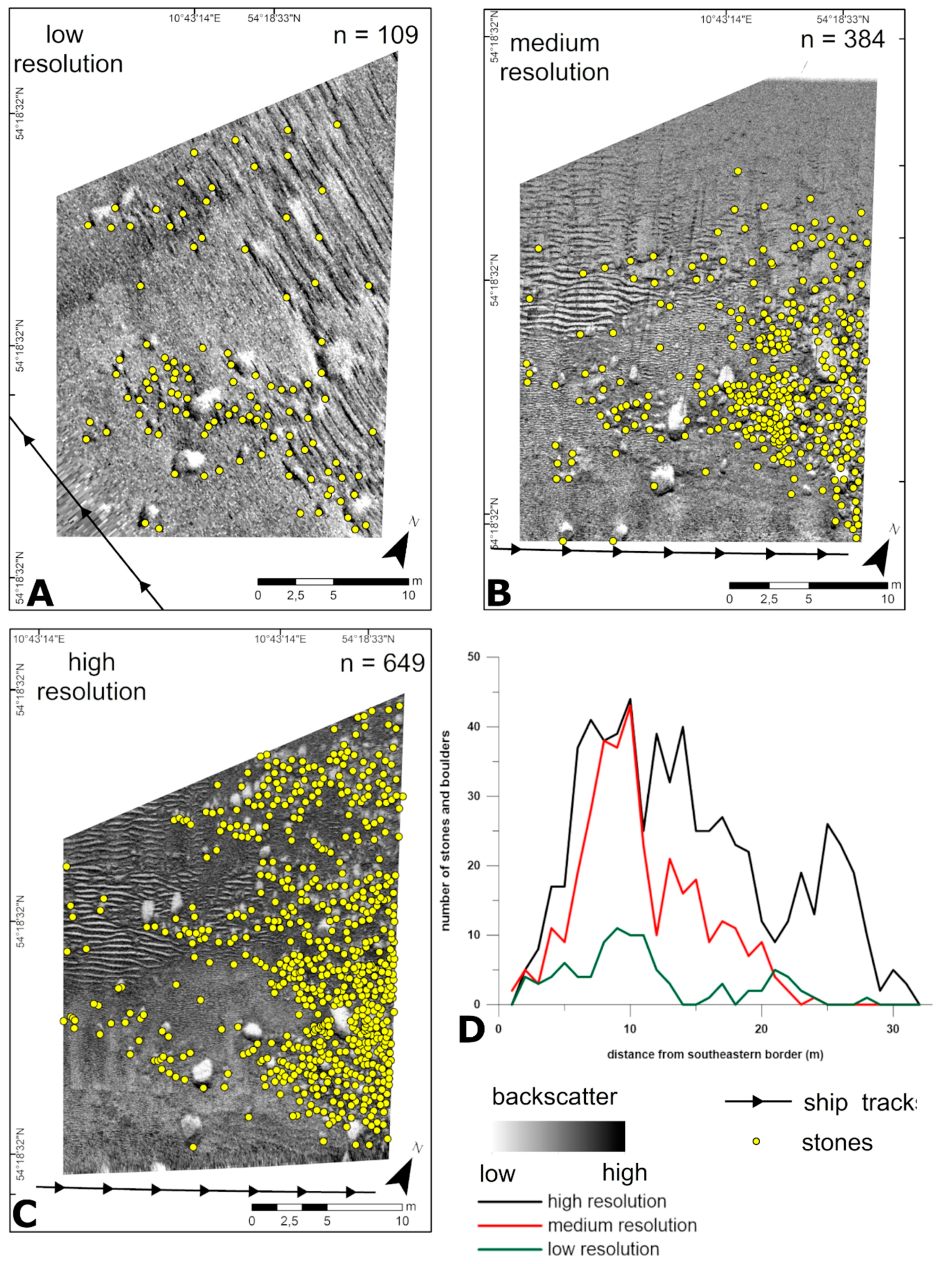
Figure 5.
Medium-resolution SSS images of the study area. Yellow dots represent detected boulders. (A–D) The four images are generated with four different approach positions and angles.
Figure 5.
Medium-resolution SSS images of the study area. Yellow dots represent detected boulders. (A–D) The four images are generated with four different approach positions and angles.
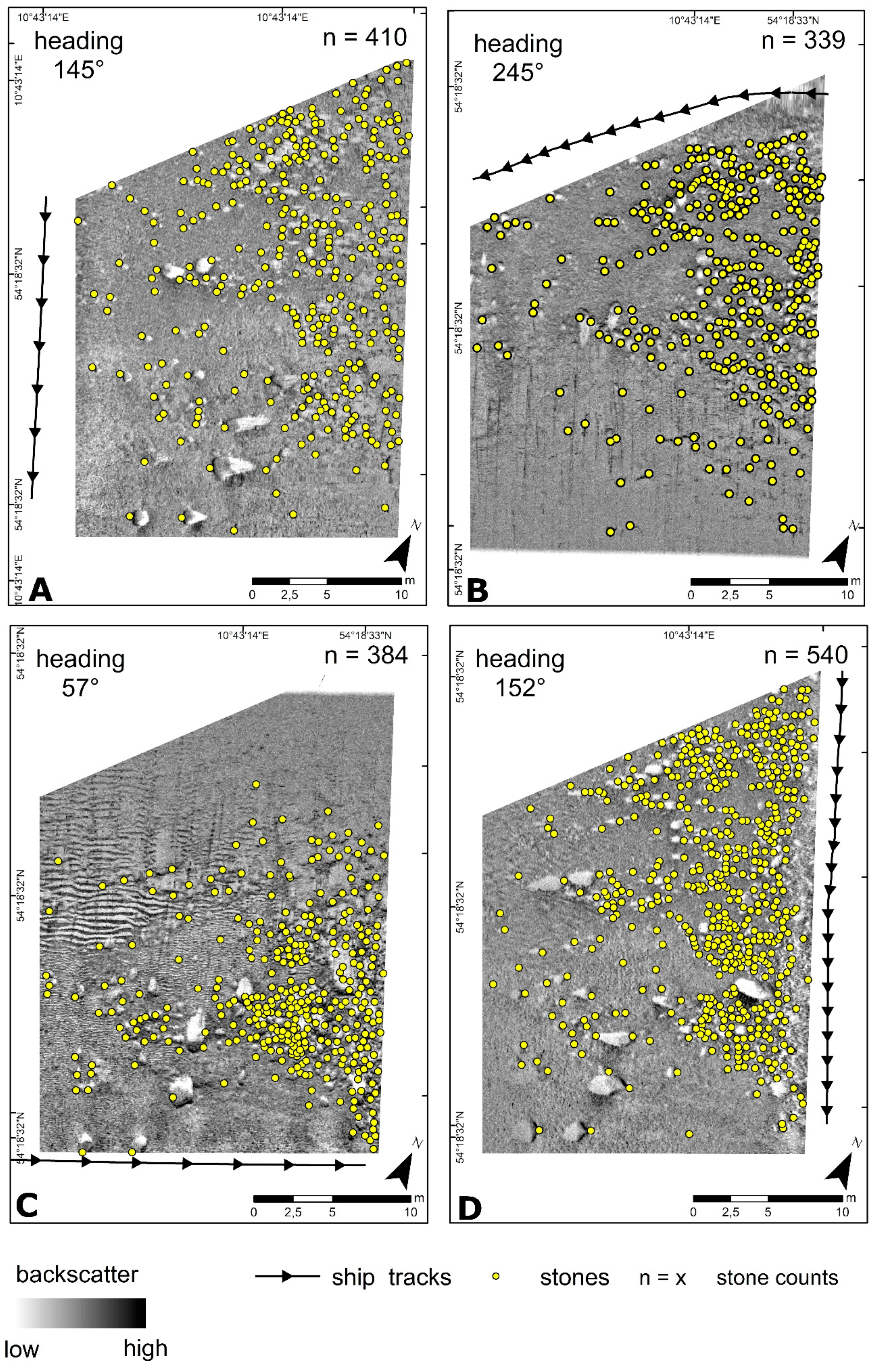
Figure 6.
High-resolution SSS images of the study area. Dots represent detected boulders. The images A–D are generated with different headings and indicate different numbers of boulders.
Figure 6.
High-resolution SSS images of the study area. Dots represent detected boulders. The images A–D are generated with different headings and indicate different numbers of boulders.

Figure 7.
Numbers of boulders: for the high and medium resolution data related to the range distance from different directions. Black lines display the numbers of boulders collected from the high-resolution data and red lines display values derived from the medium resolution data.
Figure 7.
Numbers of boulders: for the high and medium resolution data related to the range distance from different directions. Black lines display the numbers of boulders collected from the high-resolution data and red lines display values derived from the medium resolution data.

Table 1.
Three sidescan sonar (SSS) resolution classes; acoustic parameters of the sidescan transducer and selected survey parameters.
Table 1.
Three sidescan sonar (SSS) resolution classes; acoustic parameters of the sidescan transducer and selected survey parameters.
| Parameters/Classes | Low-Resolution | Medium-Resolution | High-Resolution |
|---|---|---|---|
| transmit power | 210 dB re 1μPa @ 1m | 210 dB re 1μPa @ 1m | 210 dB re 1μPa @ 1m |
| frequency | 450 kHz chirp | 1 MHz chirp | 1 MHz chirp |
| pulse length | 400 μs | 100 μs | 100 μs |
| ping rate | 14 Hz | 23 Hz | 43 Hz |
| horizontal beam width | 0.8° | 0.3° | 0.3° |
| vertical beam width | 60° | 60° | 60° |
| selected range | 50 m | 35 m | 10 m |
| average survey speed | 2.3 m/s | 1.0 m/s | 1.0 m/s |
| heading | 294° | 058° | 060° |
| average resolution | 0.2 m/pixel | 0.1 m/pixel | 0.04 m/pixel |
| merged images | - | - | 5 images merged |
Table 2.
Minimum sizes for detection and counts of boulders for the different levels of SSS resolutions.
Table 2.
Minimum sizes for detection and counts of boulders for the different levels of SSS resolutions.
| SSS Class | Frequency | Resolution | Minimum Detection Size | Detection Numbers |
|---|---|---|---|---|
| Low resolution | 450 kHz | 0.2 m/pixel | 0.4 m | 109 |
| Medium resolution | 1 MHz | 0.1 m/pixel | 0.2 m | 384 |
| High resolution | 1 MHz | 0.04 m/pixel | 0.08 m | 649 |
Table 3.
Surface areas were calculated assuming hemispheres and average diameters are estimated using minimum detection sizes.
Table 3.
Surface areas were calculated assuming hemispheres and average diameters are estimated using minimum detection sizes.
| Numbers of Boulders for Each Minimum Detection Size | |||||
|---|---|---|---|---|---|
| 0.4 m | 0.2 m | 0.08 m | Boulder Counts | Calculated Surface Area | |
| low resolution | 109 | - | - | 109 | 41 m2 |
| medium resolution | 109 | 275 | - | 384 | 67 m2 |
| high resolution | 109 | 275 | 265 | 649 | 71 m2 |
© 2019 by the authors. Licensee MDPI, Basel, Switzerland. This article is an open access article distributed under the terms and conditions of the Creative Commons Attribution (CC BY) license (http://creativecommons.org/licenses/by/4.0/).
Share and Cite
MDPI and ACS Style
von Rönn, G.A.; Schwarzer, K.; Reimers, H.-C.; Winter, C. Limitations of Boulder Detection in Shallow Water Habitats Using High-Resolution Sidescan Sonar Images. Geosciences 2019, 9, 390. https://doi.org/10.3390/geosciences9090390
AMA Style
von Rönn GA, Schwarzer K, Reimers H-C, Winter C. Limitations of Boulder Detection in Shallow Water Habitats Using High-Resolution Sidescan Sonar Images. Geosciences. 2019; 9(9):390. https://doi.org/10.3390/geosciences9090390
Chicago/Turabian Stylevon Rönn, Gitta Ann, Klaus Schwarzer, Hans-Christian Reimers, and Christian Winter. 2019. "Limitations of Boulder Detection in Shallow Water Habitats Using High-Resolution Sidescan Sonar Images" Geosciences 9, no. 9: 390. https://doi.org/10.3390/geosciences9090390
Note that from the first issue of 2016, this journal uses article numbers instead of page numbers. See further details here.