Cryomorphological Topographies in the Study of Ice Caves


1
GIR-PANGEA-Department of Geography, University of Valladolid, 47011 Valladolid, Spain
2
Department of Expresión gráfica. Escuela Politécnica, University of Extremadura, 06071 Badajoz, Spain
*
Author to whom correspondence should be addressed.
Geosciences 2018, 8(8), 274; https://doi.org/10.3390/geosciences8080274
Submission received: 30 May 2018
/
Revised: 17 June 2018
/
Accepted: 21 June 2018
/
Published: 26 July 2018
(This article belongs to the Special Issue Glacial and Geomorphological Cartography)
Abstract
:The current interest in ice caves requires that their varied manifestations be known as accurately as possible in view of their responses to a global change and also to their great potential as paleoenvironmental witnesses. This phenomenon has been known about for a long time but is still scarcely studied from the point of view of its cryological values and the evolution and distribution of many of their morphologies. For this, the development of cryomorphological topographies from traditional techniques to geodetic surveys with different tools, including terrestrial laser scanning, is one of the most current ways to characterize and quantify this type of cryospheric phenomena. It represents a new kind of periglacial cartography whose use is feasible in spite of the difficulties these environments present.
1. Introduction
In recent years the process of mapping morphologies and geomorphological processes has allowed researchers to perform detailed analyses of the origin and possible evolution of these formations. Numerous studies detail the methodologies used in periodic data collection, which evolved as new technologies developed. In the 90s the Total Station (TS) was the foremost tool used in cartographic surveys, but at the beginning of the 2000s the use of Global Navigation Satellite System (GNSS) sensors appeared, allowing the extracted cartography to be georeferenced with greater ease. The results from both techniques are the same, the information of the terrain from the survey of single points taken in the field. Although there are differences in accuracy and operability, their results can be considered to be of equal value. In the mid-2000s two new technologies emerged, terrestrial laser scanning (TLS) and photogrammetry, which radically changed both the methodologies followed and the results obtained. The final result of both is a high density point cloud that expresses the geometry of the object analyzed in very great detail. Likewise, these new procedures allow cartographies to be performed in places where it had previously been either very expensive or physically impossible.
TLS is now used for the study of caves and galleries in order to obtain a metric cartography and to produce detailed tourist information of the site. In several studies [1,2,3] the methodology used to obtain the 3D geometry of cavities has been described in detail. The results obtained are used to map, perform 3D reconstructions and create videos and 3D models for use in tourism. Idrees and Pradhan [4] detail the history of the TLS technique, the media used up until 2011 and the implementation of these in the cartographic survey of caves. The authors describe the instruments in use from the first scanner in 1998 to the equipment in use in 2011, and from that year to 2017 the technology continued to evolve with equipment of greater power and of smaller size and weight.
In spite of these developments, photogrammetry applied to the topography of caves is a difficult task, one of the main problems encountered being the need for adequate and uniform illumination throughout the cave. The metric property of the technique depends mainly on three factors: the photographic device used and the calibration of the lens, the geometry of the photographic shot and the topographic support necessary for scaling and, where appropriate, georeferencing the 3D model obtained. In three caves in Bizkaia (Spain) [5] the difficulty arose at the time of taking the photographs with the required illumination. In these surveys the geometry of the caves could be reproduced with millimetric errors and a high resolution. The technique of terrestrial photogrammetry is easier to carry out for data acquisition of small elements than large volumes. Moreau et al. [6] applied terrestrial photogrammetry inside caves in order to generate 3D reproductions of small sections of cave walls that contained traces of dinosaur tracks from the Jurassic. In some cases, it is useful to combine photogrammetry and TLS, thus allowing the documentation of a cave with difficult access and full lighting with detailed color and texture [7].
In cave topography, though on a different scale of detail, the classic survey with the disto has also now evolved. Paperless cave surveying is an example of this, a DistoX being used with the compass module and a clino (and bluetooth), pairing it with a phone, table, pda etc. and a compatible application (e.g., TopoDroid) [8].
Nevertheless, the application of these technologies to the study of endokarst cryomorphologies within ice caves has changed in recent years, and over the last decade surveys of these extreme environments have become much more scarce in comparison with those studying archaeological sites.
Although the importance of ice caves has been pointed out by many authors and its study addressed since the XVIIIth century (e.g., [9,10,11,12,13,14]), epistemological location in cryosphere sciences is still diffuse. Nowadays, there are still some research problems related to terminology (some authors refer to ice caves, glacier caves, glacières, cuevas heladas, frozen or freezing caves, ice-filled caves) regarding glacial or periglacial environment consideration and their inclusion (underground or subterranean glacier/periglacial phenomena (permafrost environment) and even some confusion regading the definition of the essential nature of the internal ice mass (stratified or not, resulting from snow, water percolation or both). Research difficulties resulting from difficult field explorations and the fact that the phenomenon is not obvious, are other important factors in this study and it is therefore also a reflection of the scarcity of TLS or photogrammetric surveys.
Also, ice caves represent the smallest ice mass in the cryosphere (ice glacier comparison mainly). Such problems make ice caves the lesser known element of the Cryosphere [15], and they are sometimes conceived as belonging to the glacial disciplines and at others periglacial, even without perennial ice masses. This obviously means that the cartography of the phenomenon is very scarce and without any consensus in the representation of its topographies and main and secondary cryological elements (both ice blocks and cryospeleothems), which are basic and essential features to establishing a common understanding.
Cartography is very useful for understanding special phenomena such as ice caves, considered to be a feature that presents huge difficulties to precise quantification due to the problems presented by cave environments. Some ice blocks cannot be seen in their entirety and others are problematic due to theie great verticality, as in the case of those located in Picos de Europa (northern Spain).
2. Study Area and Studied Topic
In this and previous studies (e.g., [16] based on previous studies mainly [12,17]) in the mountains of northern Spain, an ice cave is understood as being a cavity in which mean annual temperatures are below 0 °C with ice accumulations permanently forming stratified masses, and accompanied or not by seasonal or perennial cryospeleothems. In the cases presented in this study, these are specifically high mountain ice caves in which the accumulation of ice is mainly due to the direct input of snow under the conditions of the Atlantic humid climate characteristics of the Picos de Europa high mountain (Northern Spain) [18].
In these caves, the mean temperatures below 0 °C for more than two consecutive years lead to consider this type of cavities as periglacial representation of sporadic permafrost (already understood as such by several researchers [19,20,21] and recently noted in Picos de Europa [22,23]; and based, particularly in the last five years, on cryogenic cave carbonates as an important dating tool [24,25,26,27,28,29,30,31,32], some of them focussed on Pyrennean ice caves [33]) and even seen as a specific type of permafrost: endokarstic permafrost high mountain environment as has been considered for the Picos de Europa caves [34,35]. They are thus considered for Spanish ice caves included in endokarstic periglacial phenomena when there are at least perennial ice block, as they fulfill the thermal parameters that defines them [36], confirming the existence of permafrost high mountain environment in the calcareous mountains of the north of the Iberian Peninsula.
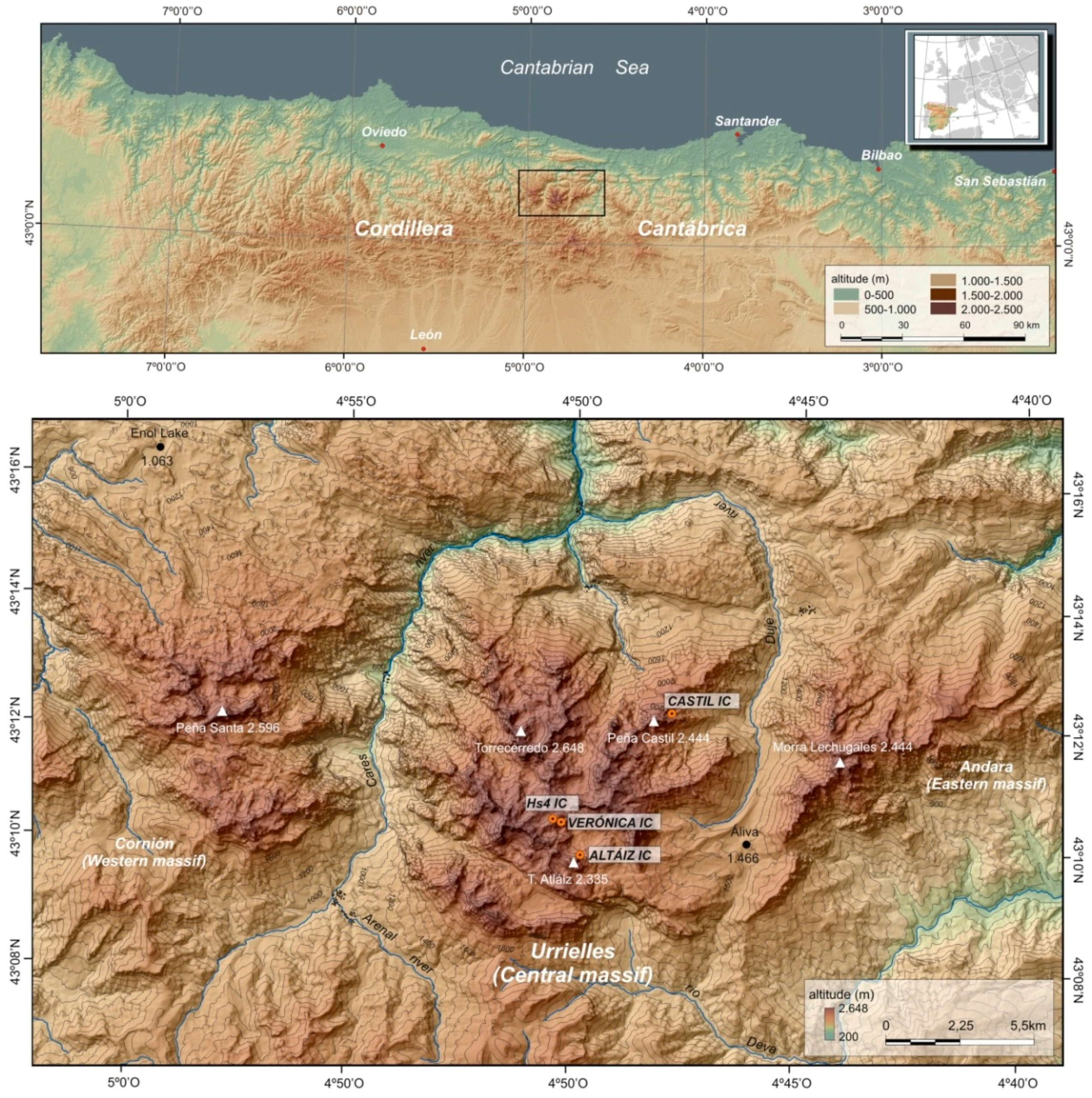
The ice caves studied here are situated in the high periglacial mountain environment of the Picos de Europa, an example of the Atlantic glaciokarst high mountain located in the north of the Cantabrian Range (northern Spain) with a maximum altitude of 2648 m.a.s.l. (Torrecerredo) (Figure 1). The current morphodynamic of this landscape (above 1800 m.a.s.l.) is dominated by snow, cold and slope dynamics. It is a marginal periglacial and totally deglaciated landscape in which the entire perennial ice body has great relevance both at the surface (perennial snow and ice patches from the glaciers of the Little Ice Age) and below it (ice caves, also from the LIA).
Picos de Europa is one of the calcareous massifs with the highest concentration of vertical caves in the world. The geostructural arrangement of large accumulations of carboniferous limestones, together with the aforementioned Atlantic climate, also means that 14 of them have been documented to date as cavities of over a thousand meters depth from an approximate total of 3300 caves documented throughout Picos de Europa, which has become an attraction for many cavers from all over the world since the last quarter of the 20th century [22]. This gives an idea of the endokarst importance of these mountains and the difficulty facing their study and geodetic surveys. Of the total, approximately 125 are ice caves according to a preliminary inventory currently being carried out [37]. These caves, in conjunction with some sporadic ones located in the rest of the Cantabrian Mountains (such as Grajera, Espigüete and others) and another broad representation in the Pyrenees high mountain [38,39], are the only representatives, sensu stricto, of ice caves in Spain.
In spite of this, the studies available for the Picos de Europa, on ice caves researched in this work, are very current [40], and focus nowadays on different topics by means of the continuous monitoring of five experimental caves of the Central Massif: Peña Castil, Verónica, Hs4, Altaiz, Torca de la Nieve ice caves. Three of them are presented here: Peña Castil ice cave, Altaiz ice cave and Verónica ice cave.
3. State of the Art in Ice Caves
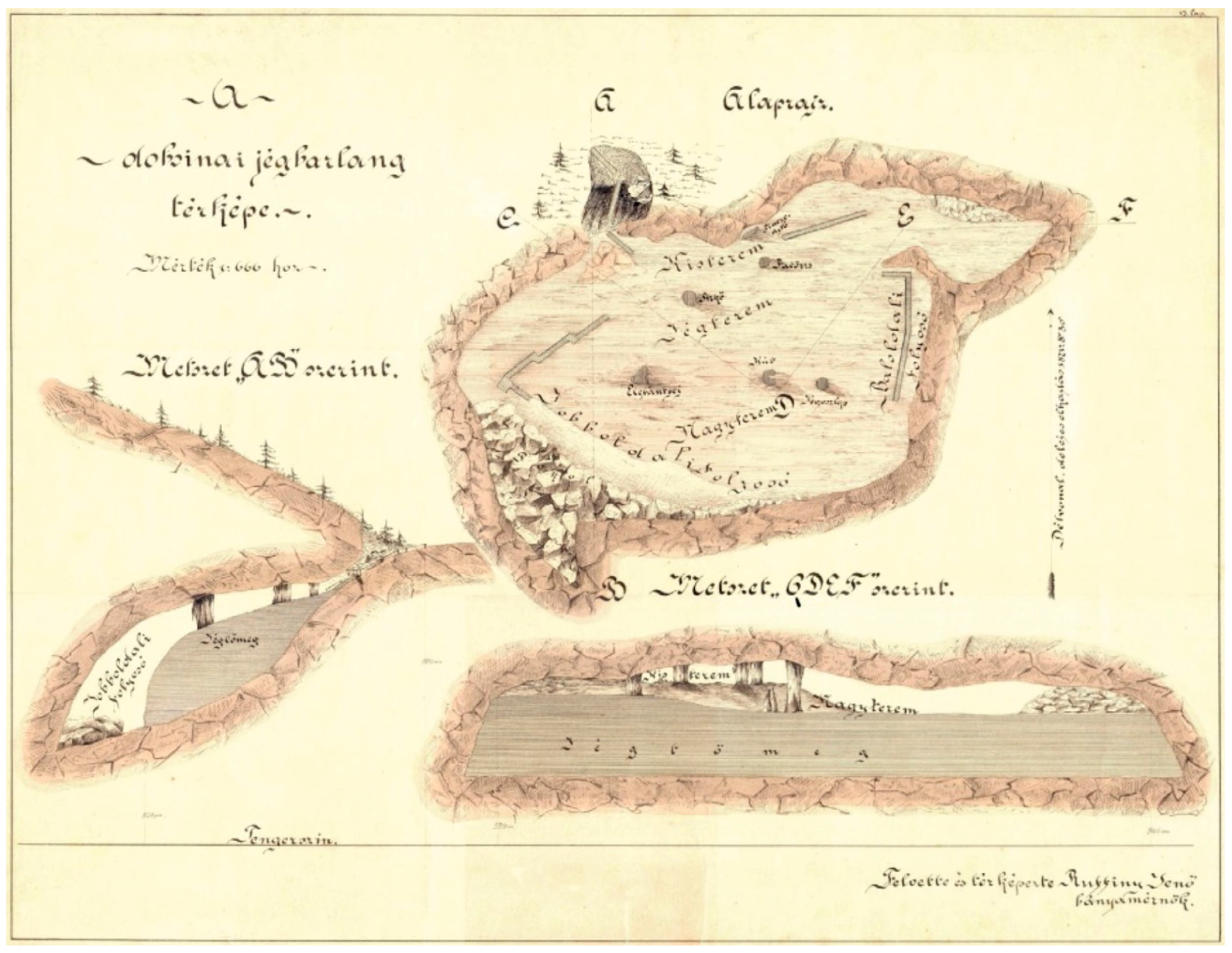
Manual and visually interpretive drawing has traditionally been used to implement topographies and cartographies of ice caves, as it has in many geomorphological, glacial and periglacial studies on the surface. Historical sources reveal topographies of caves with internal ice drawn and colored, in some cases masterfully, and in which only occasionally, for specific renowned caves (e.g., Scărişoara or the Besançon famous ice caves since XIX), certain types of ice morphologies were differentiated. They were topographies in which some manually measured data (often temperature, humidity or atmospheric pressure) were also recorded (Figure 2, Figure 3, Figure 4 and Figure 5).
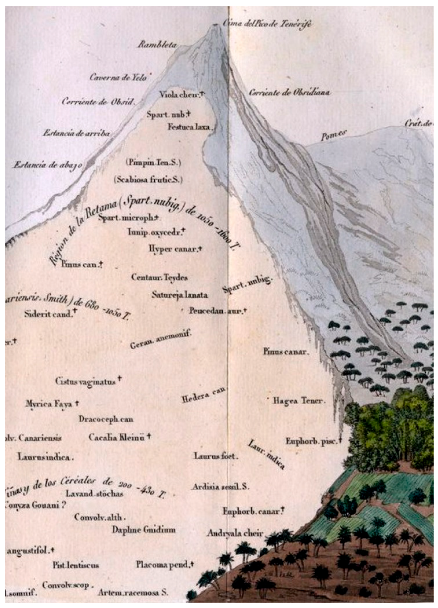
At the end of the 19th century, some qualitative advances were made regarding the equipment when making topographies, but usually they represent very specific cases, in which the ice caves are represented with very novel techniques, even if only at their mouths. For example, the astronomer Smith for the Altavista ice cave (Teide-Spain) collected the entrance mouth by means of stereoscopic photographs as early as 1865 (Figure 5), a cave previously studied by Humboldt [44] when he climbed the volcano (Figure 6).
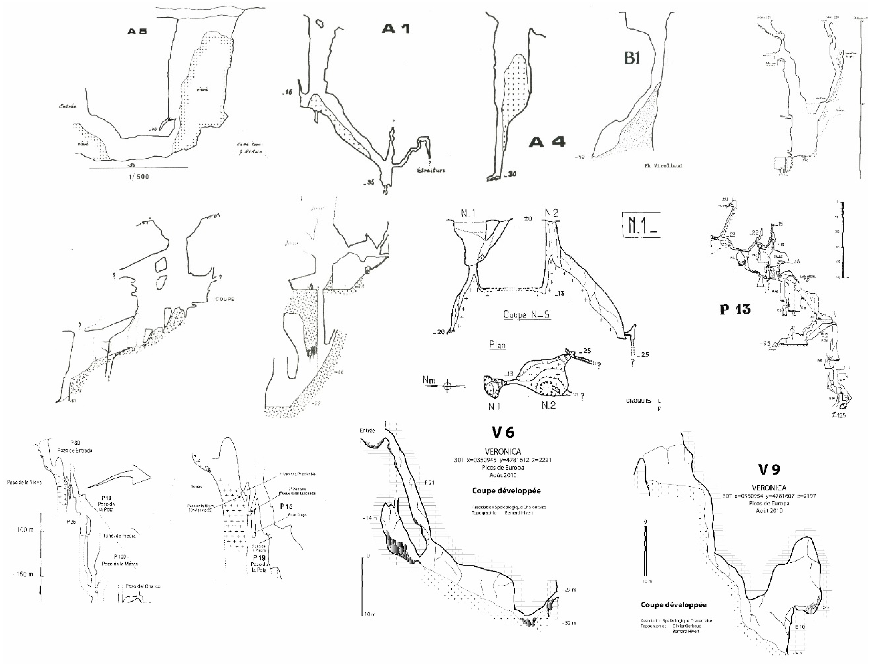
Advances in speleology and instruments have also provided improvements and made it easier to conduct topographic surveys, which has resulted in greater precision in measurements and a progressive distinction of cryomorphologies within the cavities. In the case of ice caves, however, a phenomenon that attracted little interest until the last decades of the 21st century, ice blocks (and even more so the more minor cryomorphologies such as ice stalagmites, ice stalactites, ice columns, ablation morphologies, etc.) were always represented as an undifferentiated mass of snow or ice without distinguishing what it actually was. Nor was there any interest in the vast majority of the topographies in which specific quantitative measurements were made of ice volumes and their mass balances. This makes it, nowadays (at least in Picos of Europe significantly), despite being an international, important and recognized speleological activity from the 1960’s, detailed topographies made from a cryomorphological point of view were practically nonexistent (Figure 7).
The use of equipment and methods in traditional speleotopographies (often carried out with disto laser, plumb lines, spikes) was the most habitual and continues to be so in the case of many cavities difficult to access. More recently, the introduction of new software for the digital representation of topographies, together with new tools already commonly in use in other areas of geomorphology, are beginning to be used in the study of ice caves. In this way, progressively better, more complete and more detailed topographies are being obtained of caves in general, including ice caves. Studies have already been made in which Ground Penetrating Radar (GPR) has been used to obtain ice block volumes [46,47,48,49,50,51,52,53,54,55,56,57,58,59]. In [34] have applied it for the study of the internal structure of an ice block in Picos de Europa.
Terrestrial Laser Scanner (TLS) has been used in some cases to create realistic 3D models for use in tourism, some of them for ice caves, though it has been used rather less (e.g., Eisenreiswell [60,61]; in others, it has been used for the purpose of quantitative controls to know the evolution of mass balances or mapping thermal maps [39,62] or for monitoring some ice blocks and necessary parameters of interpolation for spatial information collection with TLS [63].
Most of the focus on cartographic and topographic representation is now on ice blocks, often ignoring the existence of other minor cryomorphologies (either permanent or seasonal, pure ice or Cryogenic Cave Carbonates-CCC). Even so, these latter are very interesting and are used today as indicators for the reconstruction of paleoenvironments. And some others authors that, although more useless in this sense, are good proxies to specify and adjust thermal maps of this kind of cavities mainly following the topoclimatic bases presented by Racoviţă [64] (Figure 8).
The lack of a large consolidated corpus in these issues of ice caves also leads to many difficulties in the nomenclatures of cryomorphologies and therefore also in the semiotics that must be used for their representation. There is currently no standard classification or way in which the ice manifests itself, or how to represent or denominate it. Frequently they are conceived under general names and representations of “ice formations” to distinguish them simply from the ice blocks. However, current books such as Ice Caves [66] contribute decisively to standardize knowledge and ways of representing morphologies. In Picos de Europa, there were only elementary topographies of some ice caves (Figure 9, Figure 10 and Figure 11).
4. Materials and Methods
In the preparation of the cryomorphologial topographies of the Picos de Europa ice caves different TLS were used over the ten years. In addition to the disto and traditional drawing, the TLS technique is now used for monitoring mass balance, especially in those cavities in which the topographic survey can be carried out, though this is not usually the case. The following TLS were used:
The Leica 3D ScanStation C10 was used in the first years. It measures distances within a range of 1.5 to 300 m with nominal precision of +/− 6 mm at a distance of 50 m with normal illumination and under conditions of reflectivity. The vertical field of vision has a range of 270° sexagesimal and 360° in the horizontal. The software used for recording, alignment of clouds of points and data treatment was Leica Cyclone 7.3 ©. For the measurement of ice caves, several scans were made from each of the walls of the ice cave, which required prior planning. The placements were usually at medium resolution with a full field of vision (360° in the horizontal and 270° in the vertical), all of which lasted 7.5 min. This type of TLS wasalso used in mass balance monitoring by Gašinec et al. in the Dobšinská ice cave [63].
In later years a more modern, lighter, more precise and faster laser was used. It is a Faro Focus 3D X330, with a range of 330 m, a measuring speed of up to 1,000,000 points/second and a precision of <1 mm at distances of less than 25 m. This TLS also has a 70 MPix camera that allows 3D color modelling. In the caves, this equipment provides agility in measurement given its 5.3 kg weight and 1 kg carbon fiber tripod. From the acquisition of one or several 3D scenarios, the point cloud models obtained are useful for monitoring variations and changes in the ice mass. The software used for the recording, alignment of clouds of points and data treatment was SCENE.
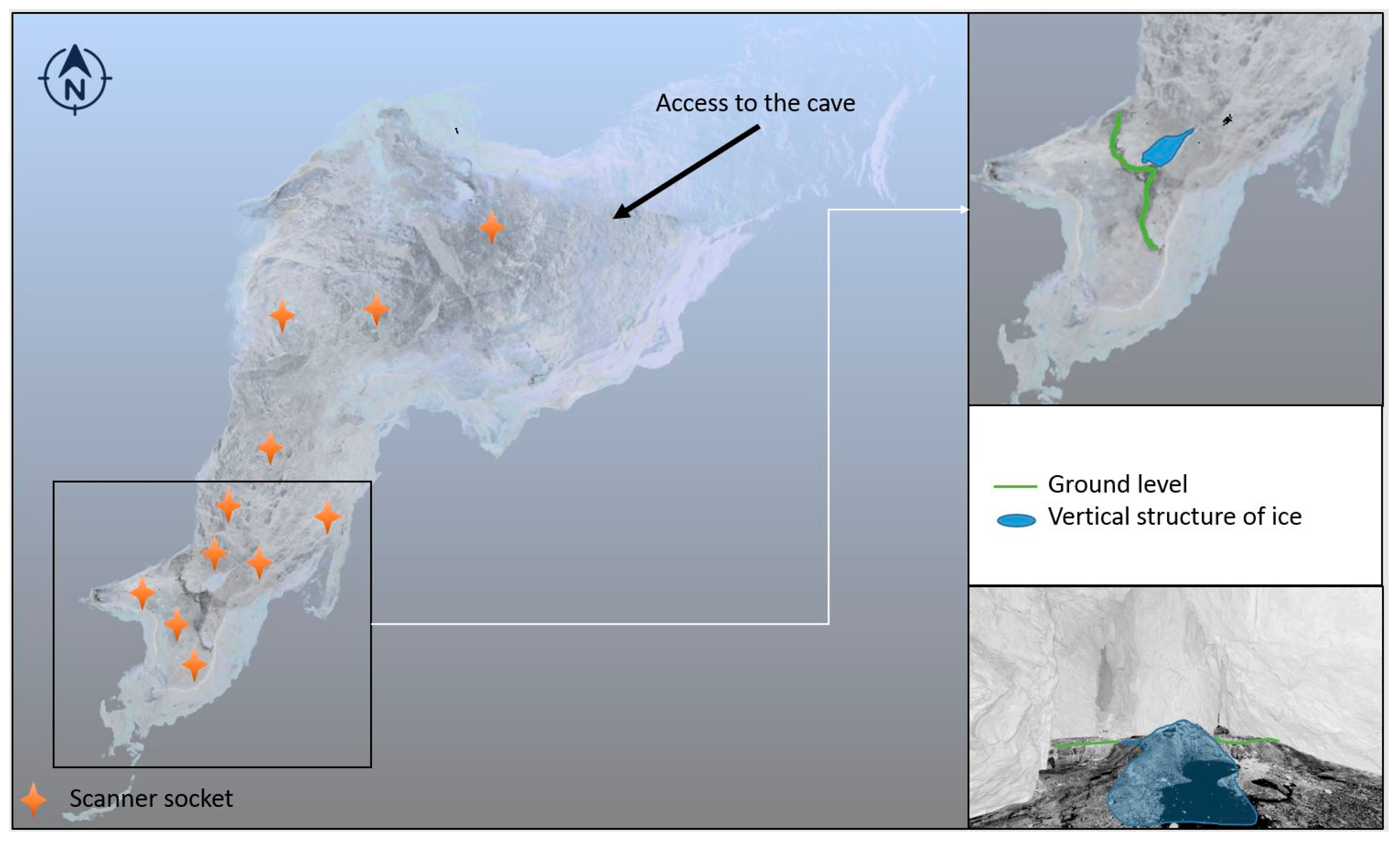
In recent years, due to the difficulty of access to the entrance of the cavity and the lower weight of the TLS, scans are being made with this latter equipment. For the complete survey of the cave, 11 outlets are made on the floor, distributed as shown in Figure 12. The aim was to connect the scans taken using the “cloud to cloud” procedure, for which sufficient coverage between shots must be considered in order for the software to be able to join them. At the time of collecting the data in the cave two geometric barriers were found in the south-western area that necessitated a greater number of shots (Figure 12). These were a vertical slope on ice ground and a small ice column in the middle of a slope.
The parameters to take into account in the Faro survey were resolution and quality. Resolution is a parameter expressed according to the distribution of points arranged in a quadrangular grid perpendicular to the scanner located at 10 m. Accuracy is an internal parameter of the equipment expressed from 1X to 8X. The manufacturer recommends a pressure of 3X for scanning interiors whose walls are >20 m. Scan timing depends directly on the parameters used. Table 1 describes the combination of parameters and times used in data collection. The resolution ranges that facilitated the most productive work were those set to 1/5 and 1/4. The equipment was configured at 1/4 resolution and 3X accuracy, thus ensuring a high level of detail, which is necessary if the automatic connection is not made and sufficient precision is to be achieved.
The shots were joined using the SCENE software. In this case partial joints were made from nearby shots and the different groups of shots were later joined together, firstly joining groups of independent clusters and then joining the clusters together.
4.1. Automatic Cameras
Cameras traps mod. Bushnell Trophy Cam XLT installed in the cavities enabled the distinction of some seasonal cryomorphologies that are difficult to discern in volume and evolution during certain seasons of the year (in winter mainly due to the dangerous access to some cavities). From these cameras a photograph is obtained every four hours and can keep a temporary record of some very specific forms. It is even able to work in conditions of total darkness. These images complement the cartography of the cavities when field work cannotbe done.
4.2. Cryomorphological Topographies Legend
In conjunction with the geodesic survey, modelling and differentiation in the field of the different types of cryomorphologies and their subsequent expression in the cryomorphological topographies of the ice caves, a classification of morphologies was established according to different criteria. This is an essential task requiring prior planning of the terminology and semiotic to be used together with a search of the scientific literature and research in order to adjust to and maintain coherence with the few studies that have been previously made (mainly [67,68,69,70]).
In this way, colors and graphics were adapted to the different cryospeleothems identified in different caves and at different times of the year (up to 30 different morphologies in classifications present in previous studies of the ice caves of Picos de Europa [71]).
A first primary classification was established, which distinguished between ice blocks (with a fairly standardized symbology of representation and also widely used in classic cave topographies), understood as stratified ice masses of fundamentally snowy origin and metamorphic nature (firn), and other morphologies of non-stratified and usually smaller ice, denominated cryospeleothems.
Likewise, these cryospeleothems were differentiated in three large groups: accumulation morphologies, ablation morphologies and mixed genesis morphologies, and within each depending on the intensity and type of process that gave rise to them: ice recongelation, drip, flows, laminar flows, hoarfrost, air flows, standing water, etc. All ice morphologies were represented in blue tones (following shades and colors habitually used in cartographic representations of glacial geomorphology, especially periglacial), while those related to snow were represented in purple tones. In both cases, both in nival and ice forms, the topographic curves obtained in direct field surveys or through the models obtained with TLS were represented (e.g., ice block flow waves obtained in the Peña Castil ice cave by the TLS survey, which were impossible to distinguish by field inspections). Another type of morphology, indirectly related to the cold processes inside these cavities, is represented in brown tones (debris or clast accumulation, etc.). The dark lines (black and gray) were used mainly for the traditional topography representation of the caves (Figure 13).
5. Results and Discussion
5.1. Tridimensional Models Derived from TLS Surveys
The models from the TLS surveys have high resolution and are highly versatile since they are practically full spheres (the only areas unscanned are the scanner sockets). Minimal details are collected of the evolution of both the ice block and the cryospeleothems. In addition to collecting all the possible information of the volumetry of each of the scanned rooms including the walls of the ceiling, of which topographies are usually impossible to get using traditional procedures.
As a result of the methodology used, all the shots made in the field can be joined to obtain 3D models of millions of points (375 million points in the case of the last scans made using the TLS Faro). When the “cloud to cloud” method is used for this task, the precision of the join is expressed as a percentage of the coverage, a percentage of the points in the bonded coverage with an accuracy <4 mm and an average of all the points computed to make the joint. The error of the joint of the cave as a whole was 6.77 mm on average with an overlap of 34.9% between clusters, whose accuracy is <4 mm in 30.8% of the joint (Table 2).
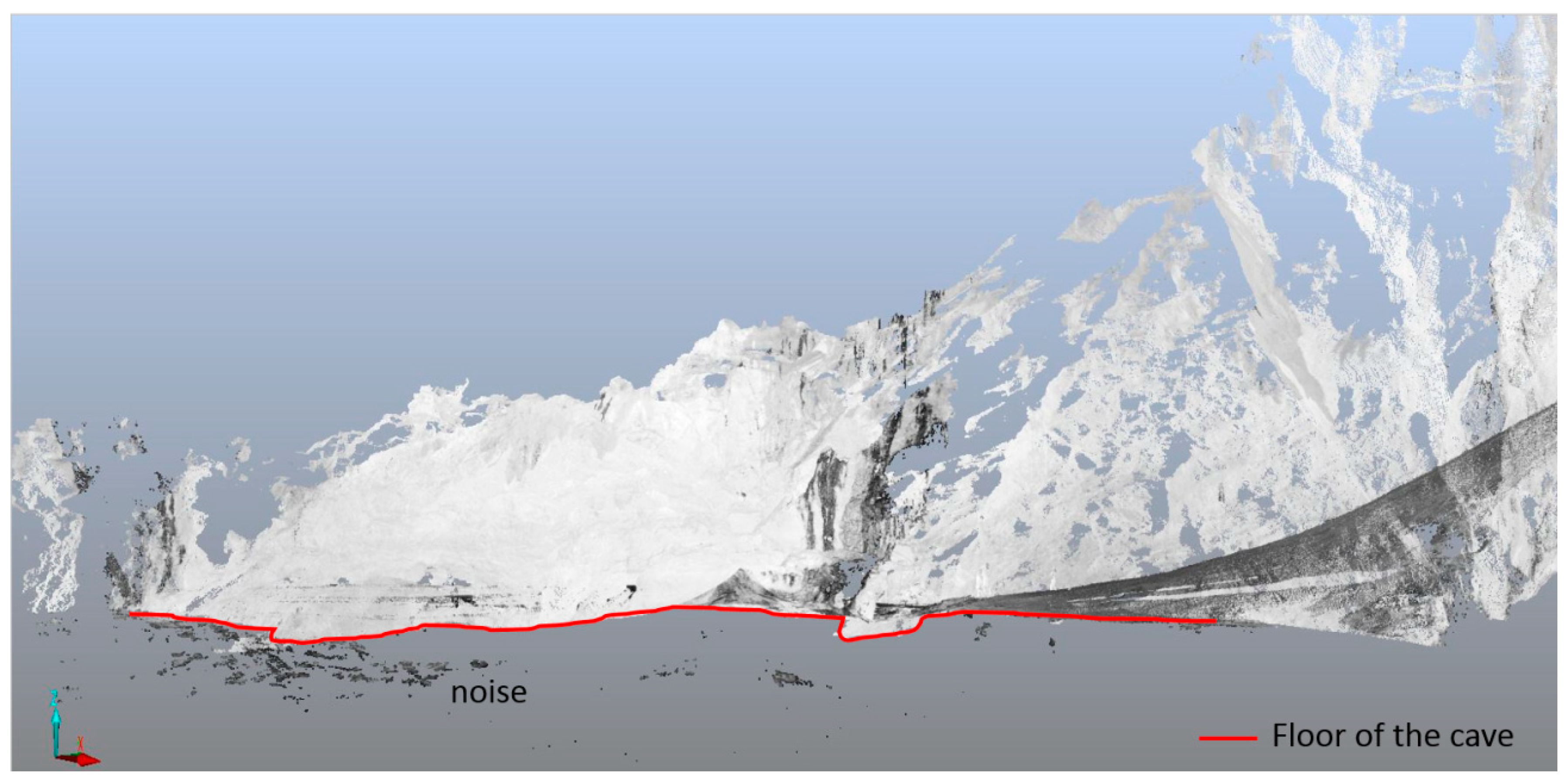
A controversial feature of this type of cave is the ice floor. At the time of the laser scan, the possibility of noise around the ice is known, so the error in the points that define the geometry of the ice is greater than the rest. Figure 14 shows a side view of the cave in which the noise appearing on the Peña Castil ice cave floor, due to the mirror effect of ice, can be seen. The scanner calculates the point cloud from three data: the horizontal angle, the vertical angle and the distance. The error appearsbecause the mirror effect of the ice means that the laser beam emitted by the team bounced off the ice, travels to the opposite wall of the cave and returns to the equipment by the same route. The resulting distance reading will be greater than the real one and therefore generates points according to the reading of the direction, equipment—floor, but below the latter. A similar effect also occurs in the calculation of the distance when it encounters water, in this case due to the change in the propagation medium of the beam, from air to water and back to air. This effect can appear in ice caves or ice in areas where there are puddles due to thawing. These errors are easier to detect with photogrammetry, although the mirror effect is still present.
There are two ways of obtaining a 3D model without noise errors of this type. The first is the application of filters to eliminate the points considered erroneous according to the “intensity” parameter of the point cloud. The second is the manual elimination of the noise considered erroneous from each of the independent takes. The option of using automatic filters does not work well since the “intensity” value is similar for the points considered noise and those of the ice floor, and so it is difficult to establish the limit for not removing soil and leaving no noise present in the model.
The “intensity” value of the point cloud is a factor that depends mainly on the wavelength on which the laser beam is generated and emitted. The scanner emits a pulse with one intensity value and receives a pulse of a different one. The difference between the intensity value of the pulse emitted and that received depends on two factors; the distance of the object (the energy it uses depends on the distance it covers to return to the scanner) and the substance of the object (the energy absorbed depends on the type of substance encountered). In the case of the Faro Focus 3D X330 scanner the pulse is emitted at a wavelength of 1550 nm.
Two important aims are achieved by using this type of three-dimensional model; on one hand, obtaining approximate volumes of air masses is useful for the study of air flow, and thus of thermal circulations, which are important factors for the study of the thermal evolution of the cavity and monitoring the evolution of cryomorphologies; and on the other, approximations can be made of ice volumes, since in most ice caves it is impossible to see the ice blocks in their entirety (all sides).
The amount of information obtained has also enabled us to generate a digital elevation model for the cryological studies of cryomorphologies and ice blocks (Figure 15). This is a methodology that allows the different surveys to be linked, thus offering the possibility of studying the extent to which the geometry of the cave is affected by any possible melting, as well as the establishment of a cryomorphological topography in three-dimensional millimetric detail.
The great difficulty arising in this kind of survey is the characteristics of the cavity itself since some chambers are inaccessible to TLS, mainly to the Leica TLS due to its size and weight. The much smaller and lighter Faro Focus TLS opens up many possibilities for use in more complex cavities and narrower passages.
5.2. Extraction of Partial Views and Orthoimages
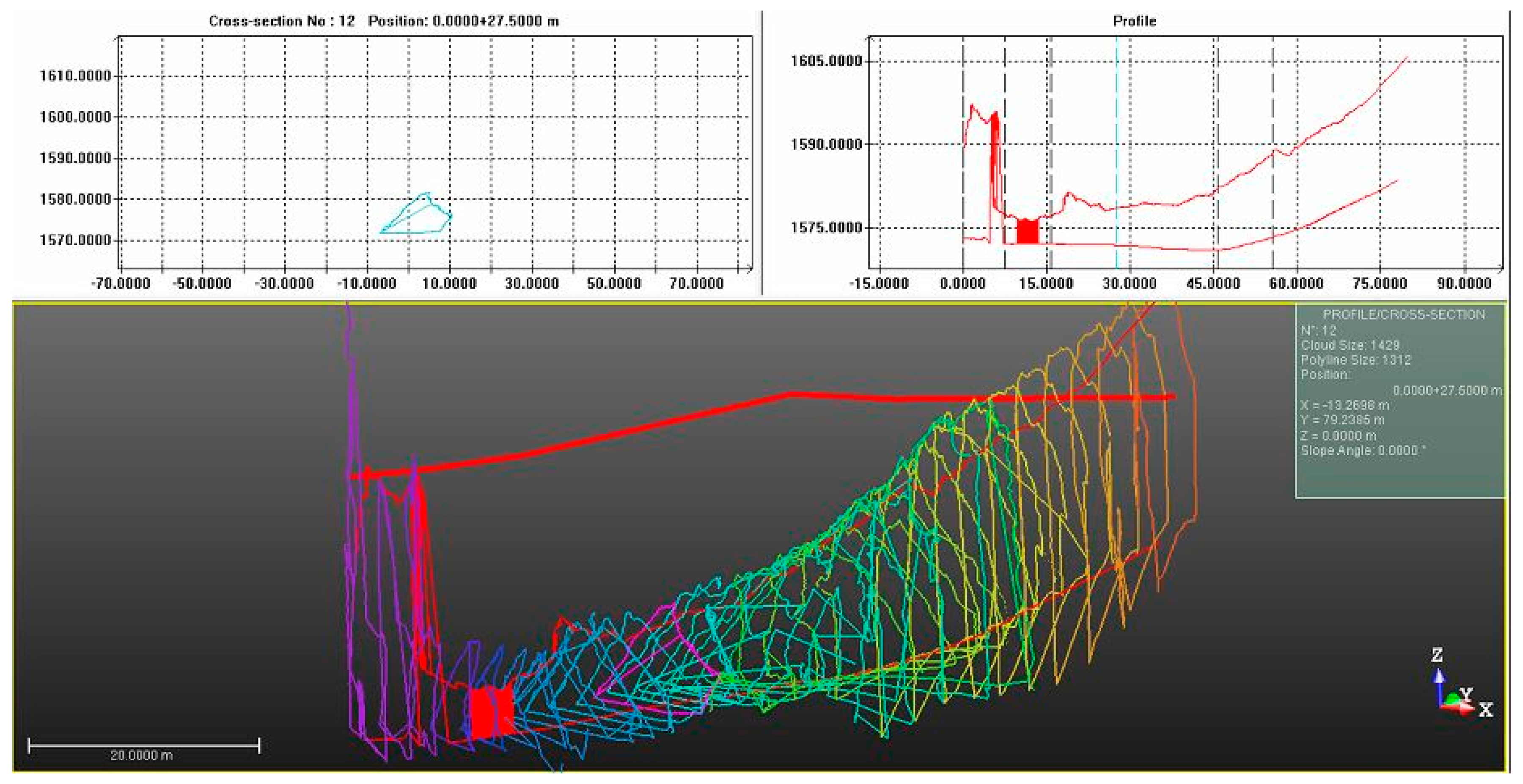
Full geometrical studies of the cavities can be extracted by 3D modelling. Transversal sections and longitudinal profiles such as those in Figure 16 have been made by means of sectioning by Real Works software.
Desired partial views are also extracted and rectified to convert them into orthoimages on which direct measurements can be made. The quantification and monitoring of almost any form within the cavity, whether an ice cave or not, is assured. There is also a great advantage in the measurement and monitoring of those more inaccessible sites such as roofs or hanging features. In some cases, scanning is combined with thermographic surveys performed with thermal cameras and more complex results are obtained in the form of orthothermographies (previously mentioned: [63]. The detection and study of air currents becomes easier with results of this nature obtained from a combination of TLS and thermographic surveys (Figure 17).
5.3. Thematic Cartographies: Temperature Maps
The results obtained with this methodology (three-dimensional models, orthoimages, thermographies or orthotermographies) facilitate the characterization of the cavities as regards the spatial temperature distribution, not only horizontally but also, and most importantly, vertically. Air pockets are sometimes detected in the roof of the cavities, which helps the vertical gradation studies. The interpolation of thermal data obtained using dataloggers permanently located in cavities is combined with the results of thermographic surveys using GIS software to obtain a continuous distribution of temperatures, the result of which is high-precision thermal maps (Figure 18).
5.4. Cryomorphological Topographies
All of these results are of importance in obtaining cryomorphological topographies. The results contain a multitude of specific details and sufficient versatility for the elaboration and rectification of cartographies with millimetric accuracy in the hostile environments posed by some ice caves (Figure 19, Figure 20 and Figure 21).
6. Conclusions
Spatial information collection and mapping of any natural element or process is now a necessary task. Virtual reality (VR) helps researchers to better understand the element studied. It provides the possibility of working on different scales and with no time limit and produces the richness of a geometric 3D model. Photogrammetry and TLS are now the techniques that enable the researcher to obtain high resolution 3D geometric models of the element surveyed. The application of these techniques requires that a series of criteria such as accessibility, dimensions and geometry, typology of the material to document and lighting be taken into account. This work presents the feasible utility of TLS in combination with other tools in the generation of precise cartographies of elements of the cryosphere, especially the most sensitive, hidden and recondite, such as ice caves.
Ice blocks cannot normally be seen on all sides, which means only estimates could previously be made of their volumes. Hence, maximum precision in the quantification of visible estimated dimensions is an important factor. Thanks to the gradual reduction of the volume of geomatic instruments, it is increasingly possible to study more complicated cavities.
Likewise, according to present global changes and the reduction of ice masses in caves worldwide, the importance of monitoring, registering and studying them from many points of view needs emphasizing in order to make reliable quantitative estimates of these ice masses and the different types of cryomorphologies that are housed within caves. Precision topography, as seen in the case presented, is of the utmost importance to this task, not only for the implementation of precise cryomorphological topographies, but also to get a standardized and usable record in combination with other methodologies for multiple objectives, such as the generation of orthoimages, orthothermographies, photorealistic models, touristic recreations, cryomorphologies classifications, etc.
Accordingly, attention must also be drawn to the need for a consensus and the standardization of the semiotics and representation symbolism of the different forms of representation of all the ice morphologies that can be found in this type of cavities, mainly due to the lack of a previous corpus in such a topic. Previous steps are needed to gain more accurate estimates and mapping of this globally distributed periglacial phenomenon with such high sensitivity and hence indicativeness to climate changes.
Author Contributions
This study was carried out by the two authors throughout different field campaigns. Subsequently, the information obtained in the field were analyzed and the TLS models and the final cartography and topographies was carried out jointly.
Funding
This research received no external funding.
Acknowledgments
Part of this research was funded by I+D+I Programme of the Ministry of Economy and Competitiviness (CGL2015-68144-R) (Spanish government). Special thanks to speleological clubs: CES-Alfa (Spain) and ASC (France).
Conflicts of Interest
The authors declare no conflicts of interest.
References
- De Sanjosé, J.; Berenguer, F.; Atkinson, A.; De Matías, J.; Serrano, E.; Gómez-Ortiz, A.; González-García, M.; Rico, I. Geomatics techniques applied to glaciers, rock glaciers, and ice patches in Spain (1991–2012). Geogr. Ann. Ser. A Phys. Geogr. 2014, 96, 307–321. [Google Scholar] [CrossRef]
- Gómez-Gutiérrez, Á.; de Sanjosé-Blasco, J.; de Matías-Bejarano, J.; Berenguer-Sempere, F. Comparing two photo-reconstruction methods to produce high density point clouds and dems in the Corral del Veleta rock glacier (Sierra Nevada, Spain). Remote Sens. 2014, 6, 5407–5427. [Google Scholar] [CrossRef]
- Gómez-Ortiz, A.; Oliva, M.; Salvador-Franch, F.; Salvà-Catarineu, M.; Palacios, D.; de Sanjosé-Blasco, J.; Tanarro-García, L.M.; Galindo-Zaldívar, J.; de Galdeano, C.S. Degradation of buried ice and permafrost in the Veleta cirque (Sierra Nevada, Spain) from 2006 to 2013 as a response to recent climate trends. Solid Earth 2014, 5, 979–993. [Google Scholar] [CrossRef] [Green Version]
- Avian, M.; Kellerer-Pirklbauer, A.; Lieb, G. Geomorphic consequences of rapid deglaciation at Pasterze glacier, Hohe Tauern range, Austria, between 2010 and 2013 based on repeated terrestrial laser scanning data. Geomorphology 2018, 310, 1–14. [Google Scholar] [CrossRef]
- Basantes, J.; Godoy, L.; Carvajal, T.; Castro, R.; Toulkeridis, T.; Fuertes, W.; Aguilar, W.; Tierra, A.; Padilla, O.; Mato, F.; et al. Capture and processing of geospatial data with laser scanner system for 3D modeling and virtual reality of amazonian caves. In Proceedings of the 2017 IEEE Second Ecuador Technical Chapters Meeting (ETCM), Salinas, Ecuador, 16–20 October 2017; pp. 1–5. [Google Scholar]
- Obradovic, M.; Abu Zeid, N.; Bignardi, S.; Bolognesi, M.; Peresani, M.; Russo, P.; Santarato, G. High resolution geophysical and topographical surveys for the characterisation of fumane cave prehistoric site, Italy. In Proceedings of the Near Surface Geoscience 2015—21st European Meeting of Environmental and Engineering Geophysics, Turin, Italy, 6–10 September 2015. [Google Scholar]
- Cosso, T.; Ferrando, I.; Orlando, A. High-precision laser scanning for cave tourism 3D reconstruction of the Pollera cave, Italy. Gim Int. Worldw. Mag. Geomat. 2015, 29, 23–25. [Google Scholar]
- Iturbe, A.; Cachero, R.; Cañal, D.; Martos, A. Virtual digitization of caves with parietal paleolithic art from Bizkaia. Scientific analysis and dissemination through new visualization techniques. Virtual Archaeol. Rev. 2018, 9, 57–65. [Google Scholar] [CrossRef]
- Balch, E.S. Glacieres, or Freezing Caverns; Allen Lane & Scott: Philadelphia, PA, USA, 1900. [Google Scholar]
- Girardot, A.; Trouillet, L. La Glacière de Chaux-Les-Passavant. Mem. Soc. Emul. Doubs 1885, 5, 449–524. [Google Scholar]
- Browne, G.F. Ice-Caves of France and Switzerland: A Narrative of Subterranean Exploration; Longmans, Green and Company: London, UK, 1865. [Google Scholar]
- Thuri, H. Etude Des Glacières Naturelles; Archives des sciences de la bibliothèque universelle: Geneve, Switzerland, 1861. [Google Scholar]
- Girod-Chantrans, J. Sur la Glacière Naturelle de Chaux, a 6 Lieues de Besançon; Journal des Mines, Prairial: Paris, France, 1796; Volume 19, pp. 65–72. [Google Scholar]
- Billerez, M. Description de la Glacière Naturelle du Comté de Bourgogne; Histoire de l’Académie Royale des Sciences: Paris, France, 1712; Volume 23, pp. 21–24. [Google Scholar]
- Kern, Z.; Perşoiu, A. Cave ice–the imminent loss of untapped mid-latitude cryospheric palaeoenvironmental archives. Quat. Sci. Rev. 2013, 67, 1–7. [Google Scholar] [CrossRef] [Green Version]
- Luetscher, M.; Jeannin, P.-Y. A process-based classification of alpine ice caves. Theor. Appl. Karstol. 2004, 17, 5–10. [Google Scholar]
- Maire, R. La Haute Montagne Calcaire: Karsts, Cavités, Remplissages, Quaternaire, Paléoclimats; Editions Gap: Challes-Les-Eaux, France, 1990. [Google Scholar]
- Gómez-Lende, M.; Serrano, E. Morfologías, tipos de hielo y regímenes térmicos. Primeros estudios en la cueva helada de Peña Castil (Picos de Europa, Cordillera Cantábrica). Av. Geomorfol. España 2010, 2012, 613–616. [Google Scholar]
- Urdea, P. Permafrost and Periglacial Forms in the Romanian Carpathians. In Proceedings of the 6th International Conference on Permafrost, South China University of Technology, Beijing, China, 5–9 July 1993; pp. 631–637. [Google Scholar]
- Ford, D.C.; Williams, P.W. Karst Geomorphology and Hydrology; Unwin Hyman: London, UK, 1989; Volume 601. [Google Scholar]
- Harris, S.A. Ice caves and permafrost zones in southwest Alberta (Eishöhlen und permafrost in Südwest-Alberta). Erdkunde 1979, 33, 61–70. [Google Scholar] [CrossRef]
- Ballantyne, C.K. Periglacial Geomorphology, 1st ed.; Wiley-Blackwell: Hoboken, NJ, USA, 2018. [Google Scholar]
- Serrano, E.; Gómez Lende, M. Underground permafrost conditions in Picos de Europa high mountain: The ice caves. In Proceedings of the 4th European Conference on Permafrost, Universidad de Lisboa-Universidad de Évora, Évora, Portugal, 18–21 June 2014. [Google Scholar]
- Žák, K.; Onac, B.P.; Kadebskaya, O.I.; Filippi, M.; Dublyansky, Y.; Luetscher, M. Cryogenic mineral formation in ice caves. In Ice Caves; Persoiu, A., Lauritzen, S.E., Eds.; Elsevier: Oxford, UK, 2018; pp. 123–162. [Google Scholar]
- Obu, J.; Košutnik, J.; Overduin, P.; Boike, J.; Zwieback, S. Subterranean periglacial landforms in ledena jama pod hrušico cave, slovenia. In Proceedings of the XI International Conference on Permafrost, Universitat Postdam-Alfred Weneger Institut, Postdam, Germany, 20–24 June 2016; Universitat Postdam-Alfred Weneger Institut: Postdam, Germany, 2016; p. 77. [Google Scholar]
- Milovský, R.; Orvošová, M.; Milovská, S.; Surka, J.; Herich, P.; Biron, A.; Mikus, T. Heterochronous populations of cryogenic cave calcite may reflect depth of permafrost thawing events. In Proceedings of the XI International Conference on Permafrost, Universitat Postdam-Alfred Weneger Institut, Postdam, Germany, 20–24 June 2016; p. 331. [Google Scholar]
- Luhová, L.; Milovský, R.; Orvošová, M.; Milovská, S.; Surka, J.; Herich, P.; Chou, C.Y.; Shen, C.C. Broken stalagmites may be an indicator of permafrost thawing. In Proceedings of the XI International Conference on Permafrost, Universitat Postdam-Alfred Weneger Institut, Postdam, Germany, 20–24 June 2016. Volume Book of abstracts. [Google Scholar]
- Luetscher, M.; Hoffmann, D.; Frisia, S.; Sattler, B.; Spötl, C. Reconstructing permafrost thaw events from alpine cave systems. In Proceedings of the XI International Conference on Permafrost, Universitat Postdam-Alfred Weneger Institut, Postdam, Germany, 20–24 June 2016. Volume Book of abstracts. [Google Scholar]
- Dublyansky, Y.; Kadebskaya, O.; Luetscher, M.; Cheng, H.; Kolta, G.; Spötl, C. Tracking the southern boundary of the late pleistocene permafrost in the Ural mountains using cryogenic cave carbonates: A feasibility study. In Proceedings of the XI International Conference on Permafrost, Universitat Postdam-Alfred Weneger Institut, Postdam, Germany, 20–24 June 2016; Volume Book of abstracts. p. 319. [Google Scholar]
- Spötl, C.; Cheng, H. Holocene climate change, permafrost and cryogenic carbonate formation: Insights from a recently deglaciated, high-elevation cave in the Austrian Alps. Clim. Past 2014, 10, 1349. [Google Scholar] [CrossRef] [Green Version]
- Žák, K.; Onac, B.P.; Perşoiu, A. Cryogenic carbonates in cave environments: A review. Quat. Int. 2008, 187, 84–96. [Google Scholar] [CrossRef]
- Žák, K.; Urban, J.; Cılek, V.; Hercman, H. Cryogenic cave calcite from several central european caves: Age, carbon and oxygen isotopes and a genetic model. Chem. Geol. 2004, 206, 119–136. [Google Scholar] [CrossRef]
- Bartolomé, M.; Sancho, C.; Osácar, M.C.; Moreno Caballud, A.; Leunda, M.; Spötl, C.; Luetscher, M.; López Martínez, J.; Belmonte, A. Characteristics of cryogenic carbonates in a pyrenean ice cave (northern Spain). Geogaceta 2015, 58, 107–110. [Google Scholar]
- Gómez-Lende, M.; Serrano, E.; Jordá, L.; Sandoval, S. The role of gpr techniques in determining ice cave properties: Peña castil ice cave, Picos de Europa. Earth Surf. Process. Landf. 2016, 41, 2177–2190. [Google Scholar] [CrossRef]
- Gomez Lende, M.; Berenguer, F.; Serrano, E. Morphology, ice types and thermal regime in a high mountain ice cave. First studies applying terrestrial laser scanner in the Peña Castil ice cave (Picos de Europa, northern Spain). Geogr. Fis. Din. Quat. 2014, 37, 141–150. [Google Scholar]
- French, H. The Periglacial Environment; Wiley: Hoboken, NJ, USA, 2007. [Google Scholar]
- Gómez-Lende, M.; Serrano, E.; Sánchez Benitez, J.; Hivert, B. El hielo en el endokarst: Cuevas heladas en la cordillera cantábrica. In Ambientes Periglaciares: Avances en su Estudio, Valoración Patrimonial y Riesgos Asociados; Ruiz-Fernández, J., García-Fernández, C., Oliva, M., Rodríguez-Pérez, C., Gallinar, D., Eds.; Servicio de Publicaciones de la Universidad de Oviedo: Oviedo, Spain, 2017. [Google Scholar]
- Serrano, E.; Gómez Lende, M.; Belmonte, A.; Sancho, C.; Sánchez-Benítez, J.; Bartolomé, M.; Leunda, M.; Moreno, A.; Hivert, B. Ice caves in Spain. In Ice Caves; Persoiu, A., Lauritzen, S.E., Eds.; Elsevier: Oxford, UK, 2018; pp. 625–655. [Google Scholar]
- Gómez Lende, M. Cuevas heladas en Picos de Europa: Clima, morfologías y dinámicas. Available online: http://uvadoc.uva.es/handle/10324/16520 (accessed on 23 July 2018).
- Gómez-Lende, M.; Serrano, E.; Sempere, F. Cuevas heladas en Picos de Europa. Primeros estudios en Verónica, Altáiz y Peña Castil. Karaitza 2011, 19, 56–61. [Google Scholar]
- Cossigny, M. Suite des Observations de m. Cossigny, sur la Glacière de Besançon, Extraites d’Une Autre Leerte Écrite à m. De Reaumur le 28 Juin 1745; Memoires de mathématique et de physique: Paris, France, 1750. [Google Scholar]
- Bella, P.; Zelinka, J. Ice Caves in Slovakia. In Ice Caves; Persoiu, A., Lauritzen, S.E., Eds.; Elsevier: Oxford, UK, 2018; pp. 657–689. [Google Scholar]
- Casteret, N. Un glaciar subterráneo en los pirineos. Peñalara, Revista Ilustrada de Alpinismo, Año XV 1928, 170, 25–35. [Google Scholar]
- Humboldt, A.V.; Bonpland, A. Le Voyage Aux Régions Equinoxiales du Nouveau Continent; Libraire grecque-latine-allemande: París, France, 1816; p. 440. [Google Scholar]
- Smyth, C.P. Teneriffe, an Astronomer’s Experiment; Lovell Reeve: London, UK, 1858. [Google Scholar]
- Colucci, R.R.; Fontana, D.; Forte, E.; Potleca, M.; Guglielmin, M. Response of ice caves to weather extremes in the southeastern Alps, Europe. Geomorphology 2016, 261, 1–11. [Google Scholar] [CrossRef]
- Stepanov, Y.; Mavlyudov, B.; Tainitskiy, A.; Kichigin, A.; Kadebskaya, O. Study of multiyear ice in Medeo cave (north Ural). In Proceedings of the 6th International Workshop on Ice Caves, Idaho Falls, ID, USA, 17–22 August 2014; Land, L., Kern, Z., Maggi, V., Turri, S., Eds.; National Cave and Karst Institute: Carlsbad, NM, USA, 2014; pp. 25–30. [Google Scholar]
- Garasic, M. New Research in Cave Ledenica in Bukovi Vrh on Velebit mt. in Croatian Dinaric Karst; Land, L., Kern, Z., Maggi, V., Turri, S., Eds.; National Cave and Karst Research Institute: Carlsbad, NM, USA, 2014; pp. 31–32. [Google Scholar]
- Colucci, R.R.; Fontana, D.; Forte, E. Characterization of two permanent ice cave deposits in the southeastern Alps (Italy) by means of ground penetrating radar (gpr). In Proceedings of the 6th International Workshop on Ice Caves, Idaho Falls, ID, USA, 17–22 August 2014. [Google Scholar]
- Rojšek, D. Cave ice in Velika leden jama v Paradani, Slovenija. In Proceedings of the 5th International Workshop on Ice Cave, Barzio and Milano, Italy, 16–23 September 2012; GeoSFerA; GeoSFerA.: Valsassina, Barzio, Italy, 2012. [Google Scholar]
- Colucci, R.R.; Forte, E.; Guglielmin, M. Underground Cryosphere in the Monte Canin Massif, Alpi Giulie (Itlay). In Proceedings of the 5th International Workshop on Ice Caves (IWIC-V), Barzio (LC), Italy, 16–23 September 2012. [Google Scholar]
- Kern, Z.; Fórizs, I.; Pavuza, R.; Molnár, M.; Nagy, B. Isotope hydrological studies of the perennial ice deposit of Saarhalle, Mammuthohle, Dachstein mts, Austria. Cryosphere 2011, 5, 291–298. [Google Scholar] [CrossRef]
- Hausmann, H.; Behm, M. Imaging the structure of cave ice by ground-penetrating radar. Cryosphere 2011, 5, 329. [Google Scholar] [CrossRef]
- Behm, M.; Hausmann, H.; Weghofer, C. Thickness and internal structure of underground ice in a low-elevation cave in the eastern Alps (Beilstein-Eishöhle, Hochschwab, Austria). In Proceedings of the 4th International Workshop on Ice Caves, Obertraun, Austria, 5–11 June 2010. [Google Scholar]
- Podsuhin, N.; Stepanov, Y. Measuring of the thickness of perennial ice in Kungur ice cave by georadar. In Proceedings of the 3rd International Workshop on Ice Caves, Kungur, Russia, 12–17 May 2008; Kadebskaya, O., Mavlyudov, B.R., Pyatunin, M., Eds.; pp. 52–55. [Google Scholar]
- Behm, M.; Hausmann, H. Determination of ice thicknesses in alpine caves using georadar. In Proceedings of the 3rd International Workshop on Ice Caves, Kungur, Russia, 12–17 May 2008. [Google Scholar]
- Behm, M.; Hausmann, H. Eisdickenmessungen in alpinen höhlen mit georadar. Die Höhle 2007, 58, 3–11. [Google Scholar]
- Novotny, L.; Tulis, J. Ice filling in the dobsina ice cave. Kras Jaskyne (Liptovsky Nikulas) 1995, 1, 16–17. [Google Scholar]
- Geczy, J.; Kucharovic, L. Determination of the ice filling thickness at the selected sites of the Dobsinska ice cave. Ochrana Ladovych Jaskyn Zilina 1995, 1, 17–23. [Google Scholar]
- Milius, J.; Petters, C. Eisriesenwelt—From Laser Scanning to Photo-Realistic 3D Model of the Biggest Ice Cave on Earth; GI-Forum: Washington, DC, USA, 2012; pp. 513–523. [Google Scholar]
- Petters, C.; Milius, J.; Buchroithner, M. Eisriesenwelt: Terrestrial laser scanning and 3D visualisation of the largest ice cave on earth. In Proceedings of the European LiDAR Mapping Forum, Salzburg, Austria, 29–30 November 2011. [Google Scholar]
- Berenguer-Sempere, F.; Gómez-Lende, M.; Serrano, E.; de Sanjosé-Blasco, J.J. Orthothermographies and 3D modeling as potential tools in ice caves studies: The Peña Castil ice cave (Picos de Europa, northern Spain). Int. J. Speleol. 2014, 43, 35–43. [Google Scholar] [CrossRef]
- Gašinec, J.; Gašincová, S.; Černota, P.; Staňková, H. Uses of terrestrial laser scanning in monitoring of ground ice within Dobšinská ice cave. J. Pol. Miner. Eng. Soc. 2012, 30, 31–42. [Google Scholar]
- Racoviţă, G. La classification topoclimatique des cavités souterraines. Trav. Inst. Spéol. Emile Racovitza 1975, 14, 197–216. [Google Scholar]
- Perşoiu, A. Ice caves climate. In Ice Caves; Persoiu, A., Lauritzen, S.E., Eds.; Elsevier: Oxford, UK, 2018; pp. 21–32. [Google Scholar]
- Perşoiu, A.; Lauritzen, S.T. Ice Caves; Elsevier: Amsterdam, The Netherlands, 2018; p. 729. [Google Scholar]
- Bella, P. Glacial ablation forms in the Dobšiná ice cave (in Slovak, englishsummary). Aragonit 2003, 8, 3–7. [Google Scholar]
- Bella, P. Glaciation ablation forms in the dobšiná ice cave. In Proceedings of the 1st International Workshop on Ice Cave, Căpuş and Scărişoara, Romania, 29 Febraury–3 March 2004; Citterio, M., Turri, S., Eds.; Universitară Clujeană: Cluj-Napoca, Romania; Volume 39.
- Bella, P. Flat floor ice surfaces in ice-filled caves (dobšinská ice cave, scărişoara cave). Aragonit 2005, 10, 12–16. [Google Scholar]
- Bella, P. Morphology of ice surface in the Dobšiná ice cave. In Proceedings of the 2nd International Workshop on Ice Caves, Liptovský Mikuláš, Slovak Republic, 8–12 May 2006; Zelinka, J., Ed.; [Google Scholar]
- Gómez-Lende, M. Cuevas Heladas en el Parque Nacional Picos de Europa. Fronteras Subterráneas del Hielo en el Macizo Central; Ministerio de Agricultura, Alimentación y Medio Ambiente: Madrid, Spain, 2016; p. 254. [Google Scholar]
Figure 1.
Location of studied ice caves.

Figure 2.
In the first topographies of ice caves with scientific nature, there was already an interest in registering the different types of cryomorphologies. Topography in plan and elevation of one of the ice caves of Besançon (France). The distribution of the different ice morphologies (premieres morceaux de glace (A), nappe de glace (E, H), coulee de glace (F), plusieurs pyramids of glace (C)) with annotations of the month when they could be appreciated ([41]).
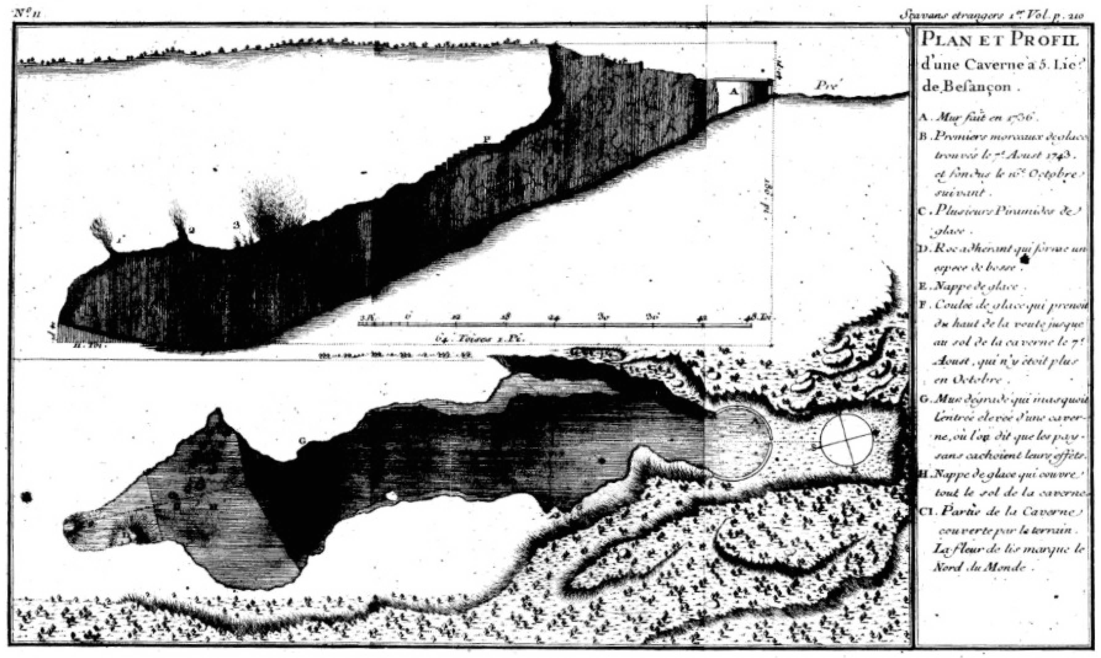
Figure 3.
Some topographies were masterfully drawn in XIX century such as Ruffíny’s map of the Dobšiná ice cave (1871) (Archive of the Slovak Museum of Nature Protection and Speleology, Liptovský Mikuláš) [42].
Figure 3.
Some topographies were masterfully drawn in XIX century such as Ruffíny’s map of the Dobšiná ice cave (1871) (Archive of the Slovak Museum of Nature Protection and Speleology, Liptovský Mikuláš) [42].

Figure 4.
One of the first topographic profiles of the Casteret ice cave (Pyrenees) [43].
Figure 4.
One of the first topographic profiles of the Casteret ice cave (Pyrenees) [43].
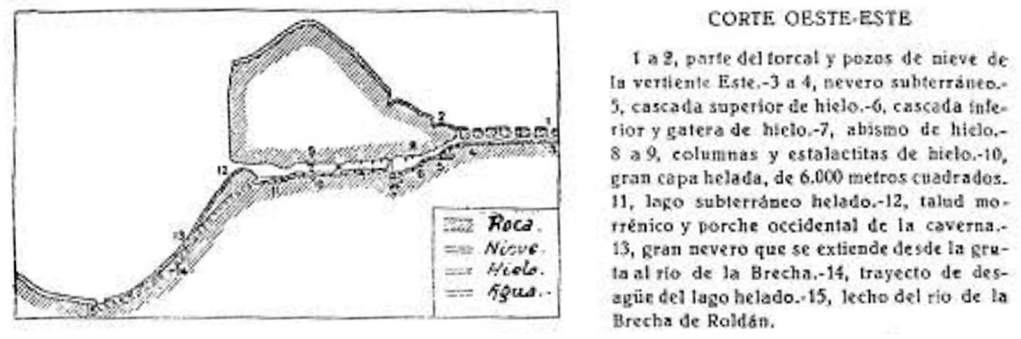
Figure 5.
Stereographic photo of the entrance and map of Teide ice cave [45].
Figure 5.
Stereographic photo of the entrance and map of Teide ice cave [45].
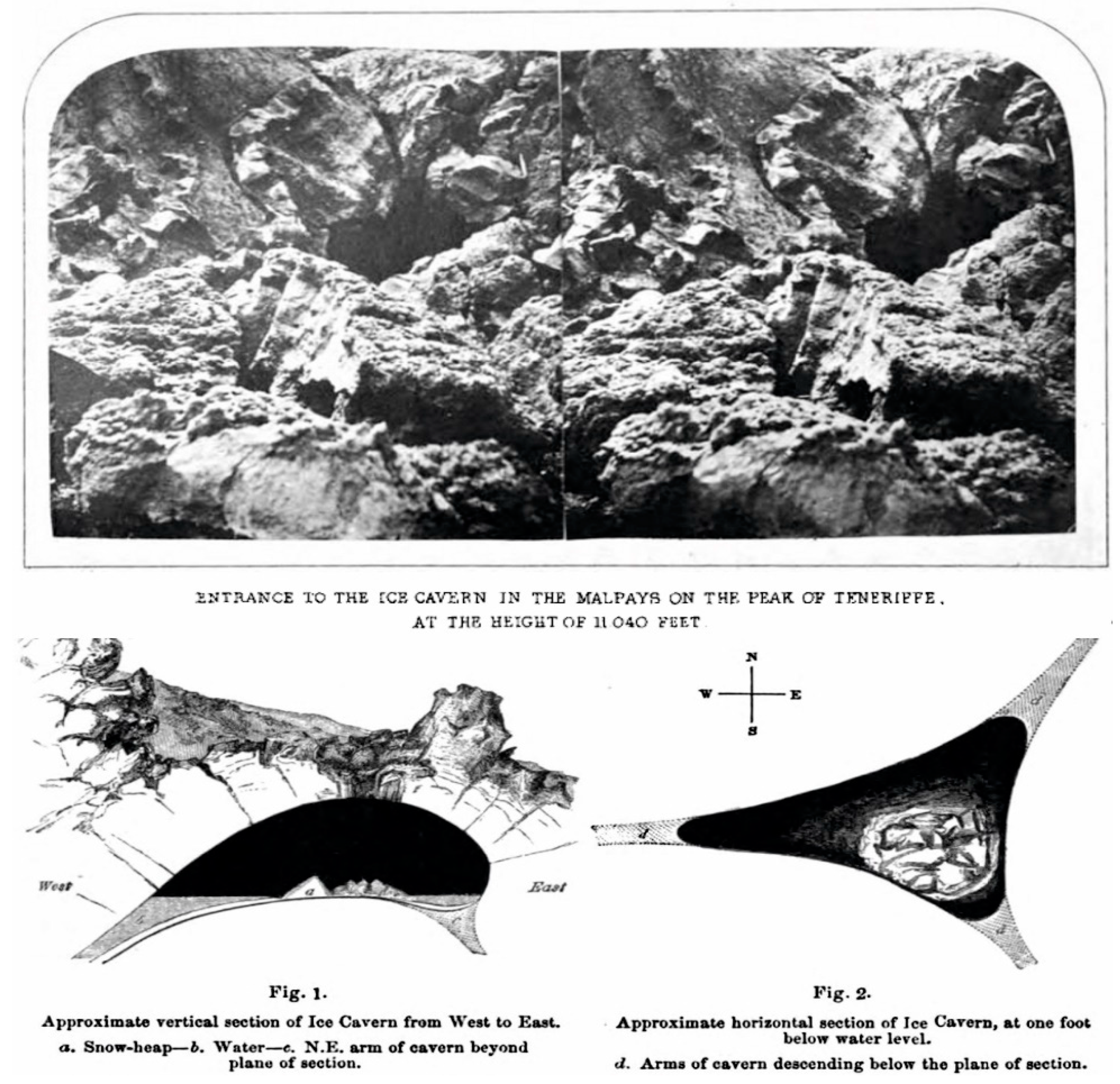
Figure 6.
The Teide ice cave represented as “Caverne du Glace” (Caverna de Xelo in the Spanish edition) in the “Tableau Physique des Isles canaries” [44].
Figure 6.
The Teide ice cave represented as “Caverne du Glace” (Caverna de Xelo in the Spanish edition) in the “Tableau Physique des Isles canaries” [44].

Figure 7.
First topographies of some of Picos de Europa ice caves (taken from ASC 1976, 1982, 2011).
Figure 7.
First topographies of some of Picos de Europa ice caves (taken from ASC 1976, 1982, 2011).

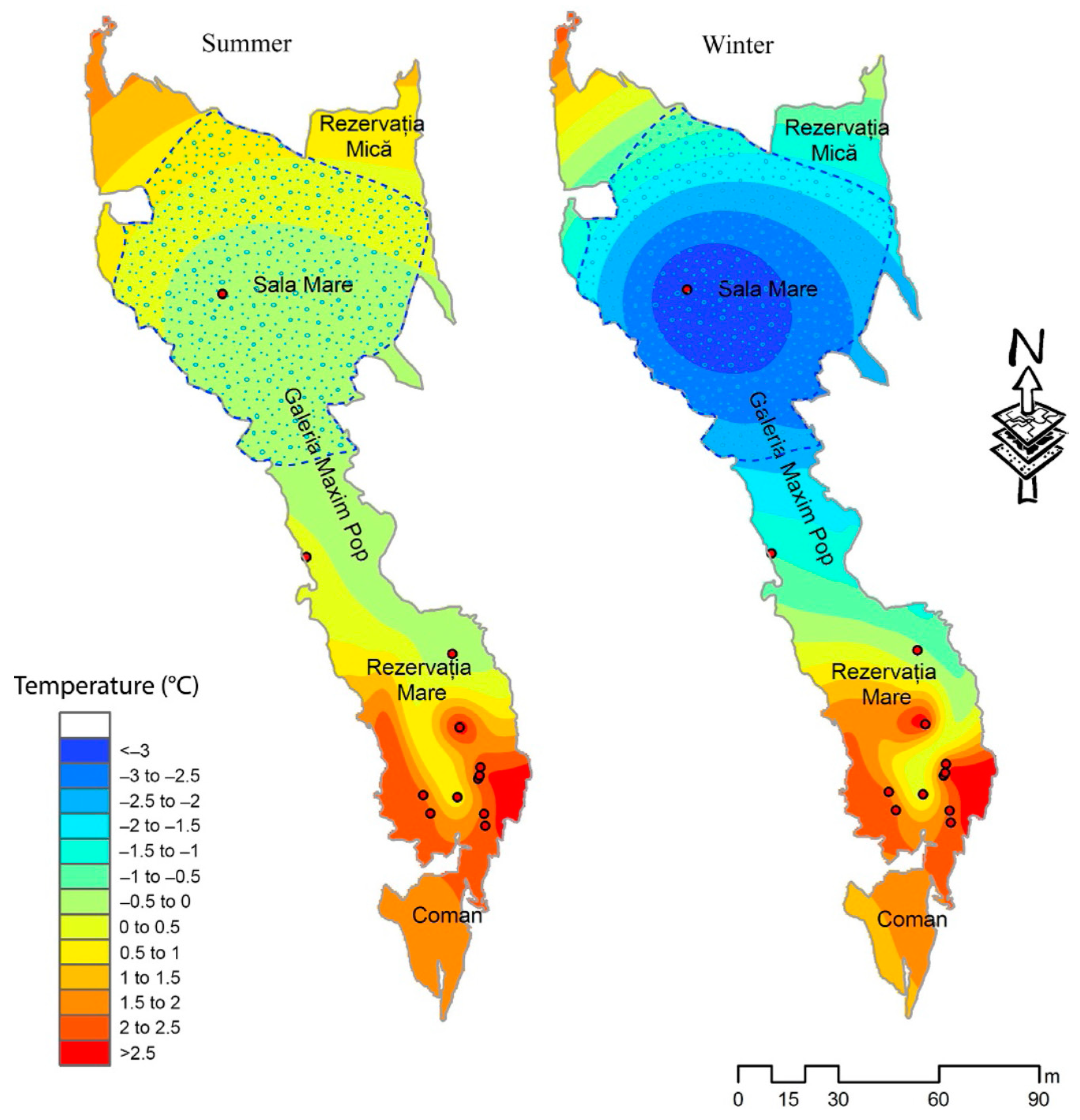
Figure 8.
Example of air temperature mapping of Scărişoara ice cave. Taken from Perşoiu [65]. The red dots are position of dataloggers (hourly air temperatures register) Map courtesy of Carmen Bădăluta.
Figure 8.
Example of air temperature mapping of Scărişoara ice cave. Taken from Perşoiu [65]. The red dots are position of dataloggers (hourly air temperatures register) Map courtesy of Carmen Bădăluta.

Figure 9.
First topographies of Peña Castil ice cave: (1) topography in 1964 (from Liautaud, 1985); (2) topographies of the GELL (1995).
Figure 9.
First topographies of Peña Castil ice cave: (1) topography in 1964 (from Liautaud, 1985); (2) topographies of the GELL (1995).
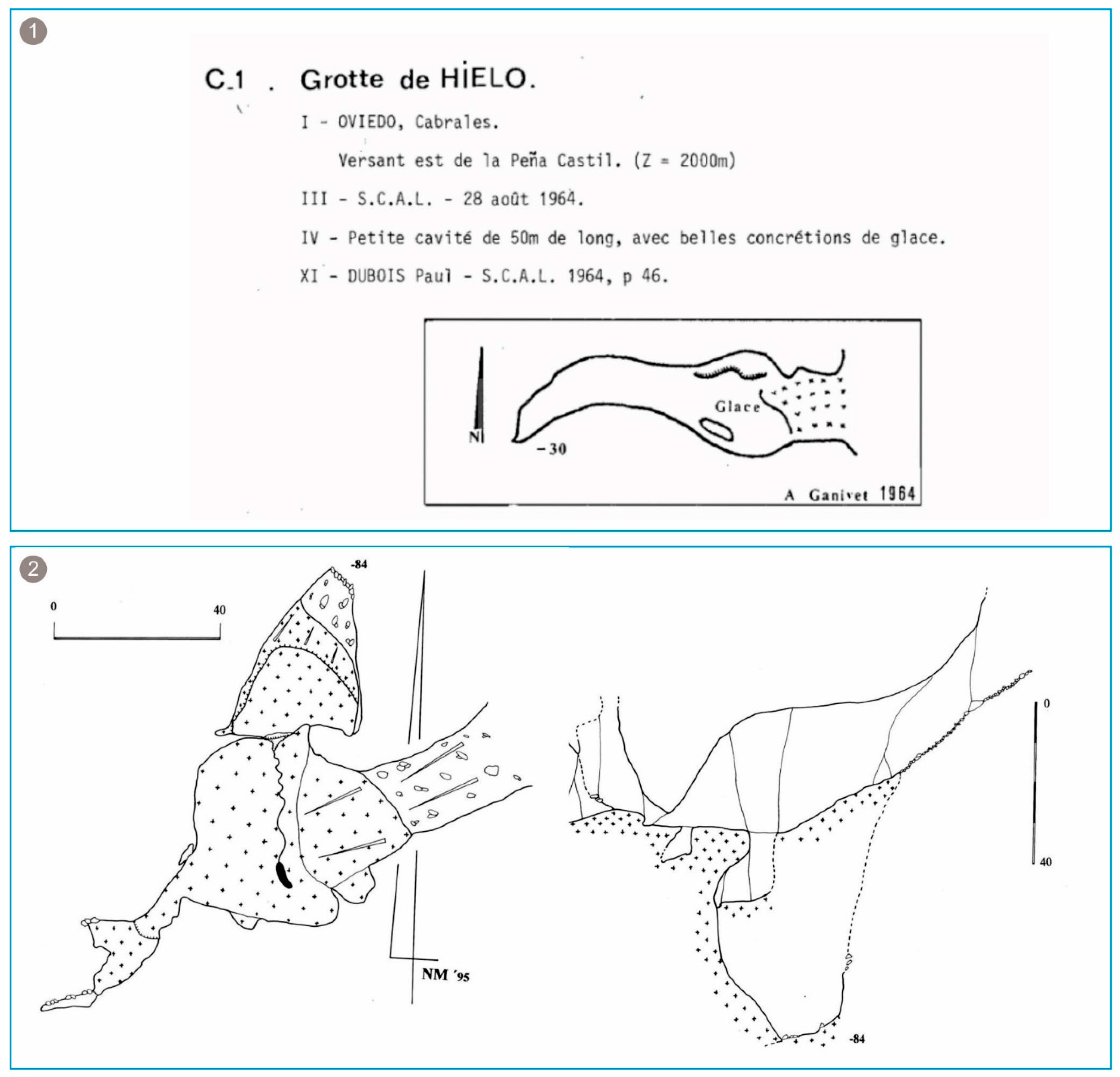
Figure 10.
First topographies of Altáiz ice cave (ASC, 1976).
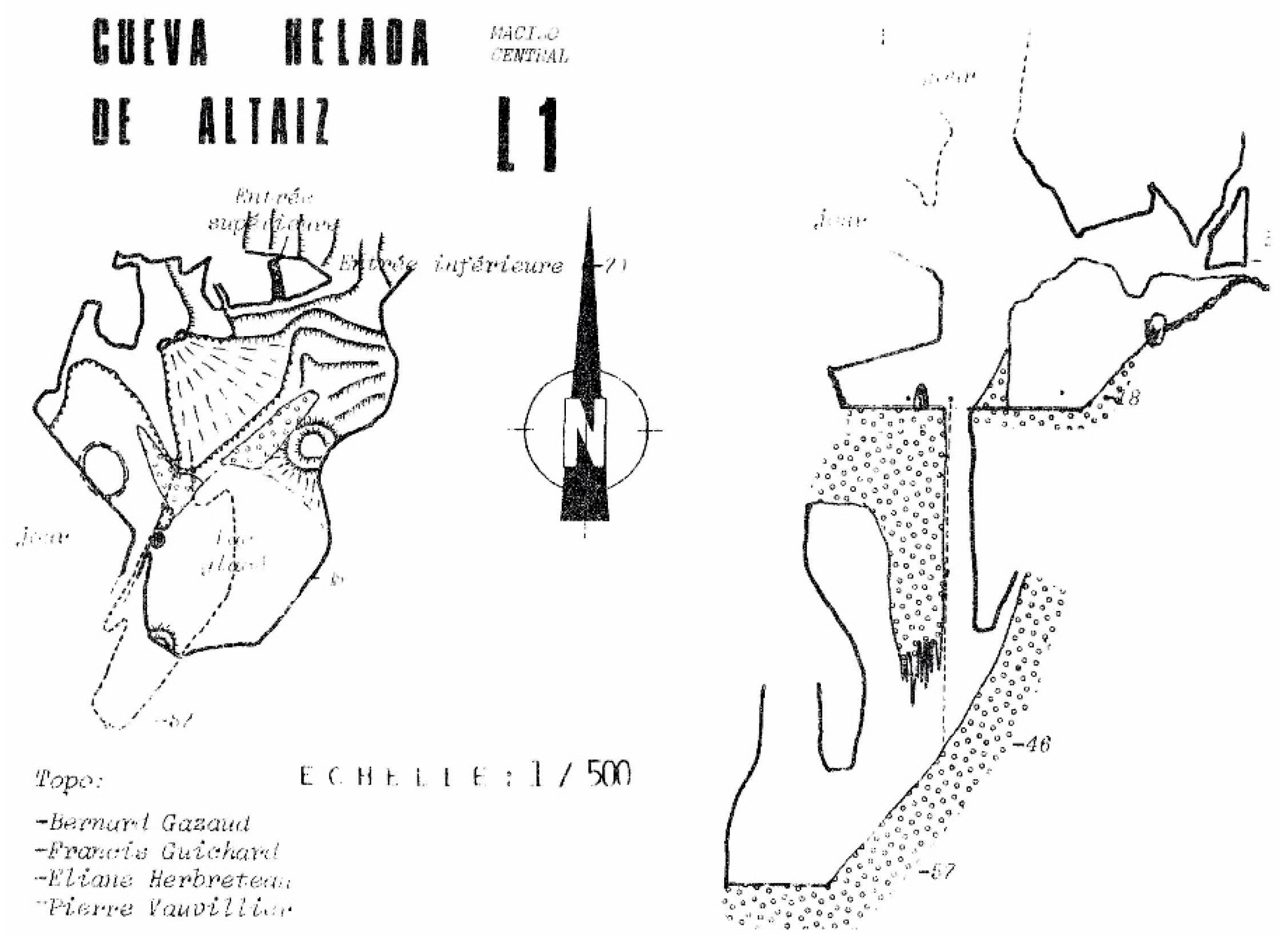
Figure 11.
Veronica ice cave topography (ASC, 2006). An improvement in the collection of cryological information is appreciated.
Figure 11.
Veronica ice cave topography (ASC, 2006). An improvement in the collection of cryological information is appreciated.
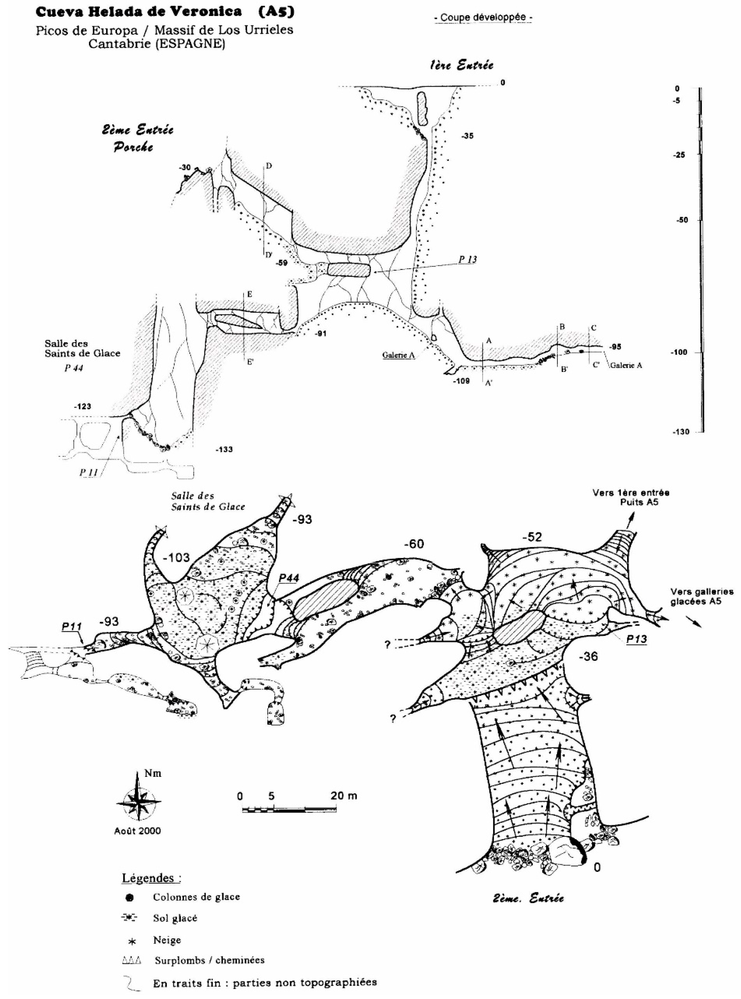
Figure 12.
Shots with TLS made in the cave and existing geometric barriers.

Figure 13.
Legend used for proposed cryomorphological topographies.
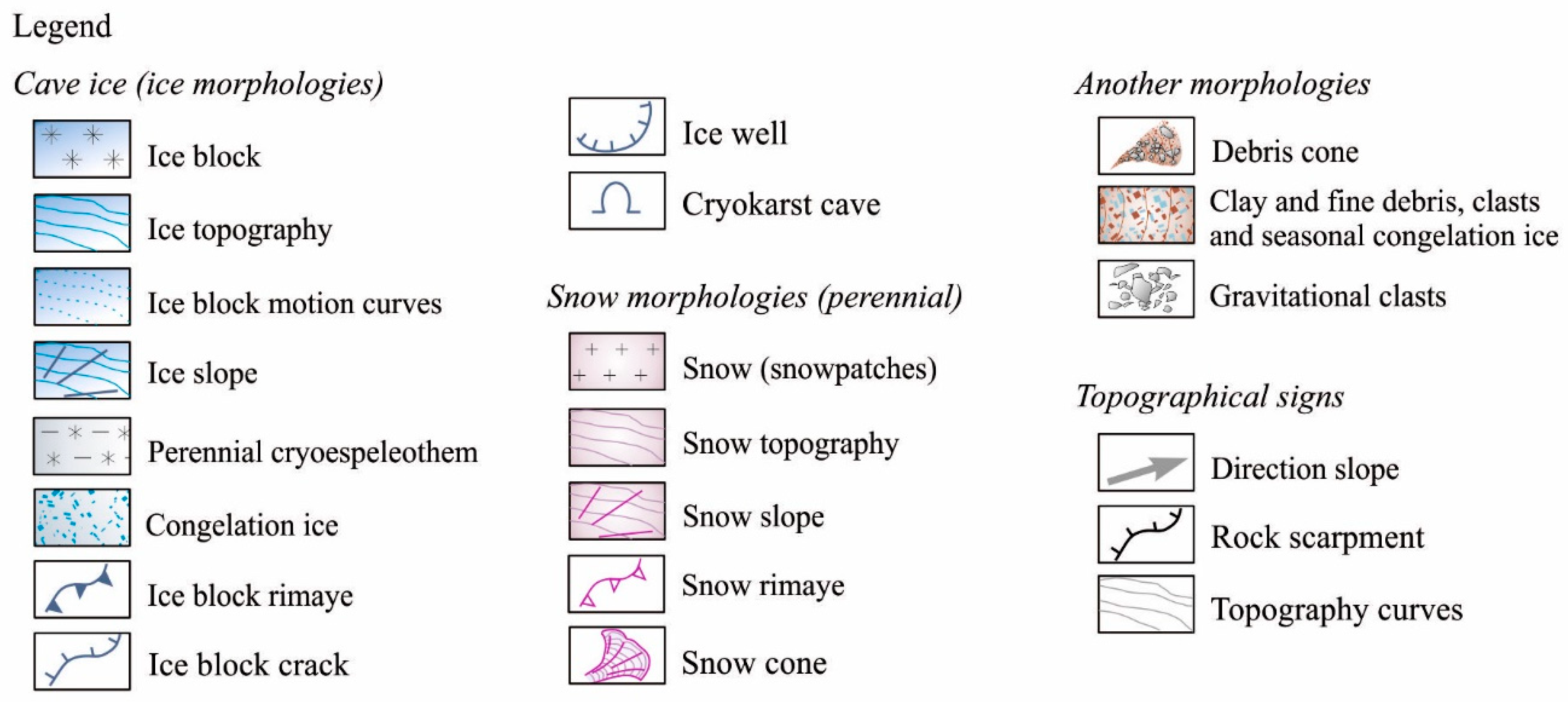
Figure 14.
Noise generated in the measurement due to the mirror effect of the ice floor.

Figure 15.
Ice block surface surveyed. Color ramp shows height from highest to lowest, yellow to dark blue respectively.
Figure 15.
Ice block surface surveyed. Color ramp shows height from highest to lowest, yellow to dark blue respectively.
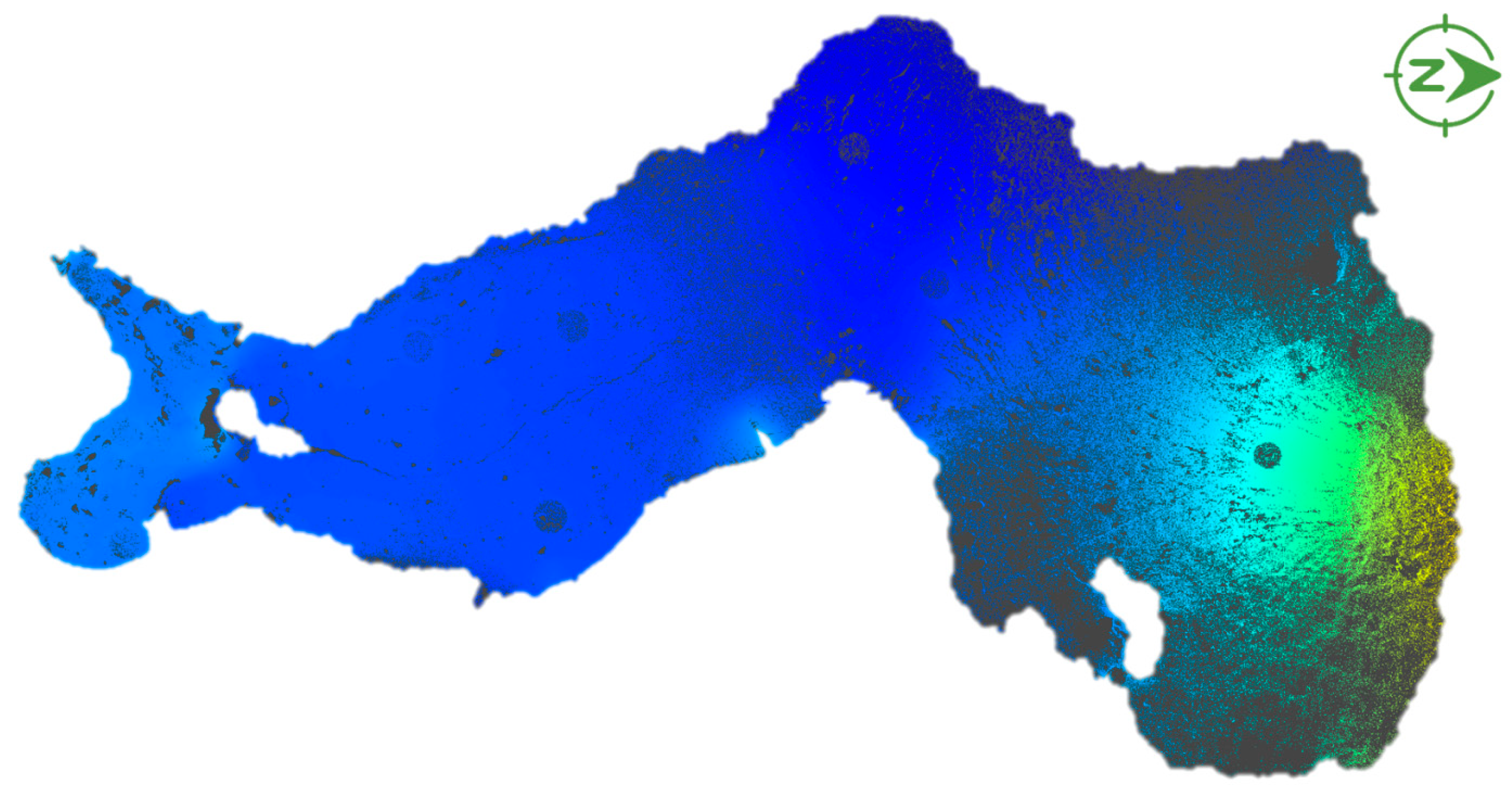
Figure 16.
Transverse and longitudinal sections of the Peña Castil ice cave.

Figure 17.
Orthothermography of one of the walls of the main ice room of Peña Castil ice cave. b, possible termperature influence of the ice block (cold halo). In yellow the targets of geodetic work.
Figure 17.
Orthothermography of one of the walls of the main ice room of Peña Castil ice cave. b, possible termperature influence of the ice block (cold halo). In yellow the targets of geodetic work.
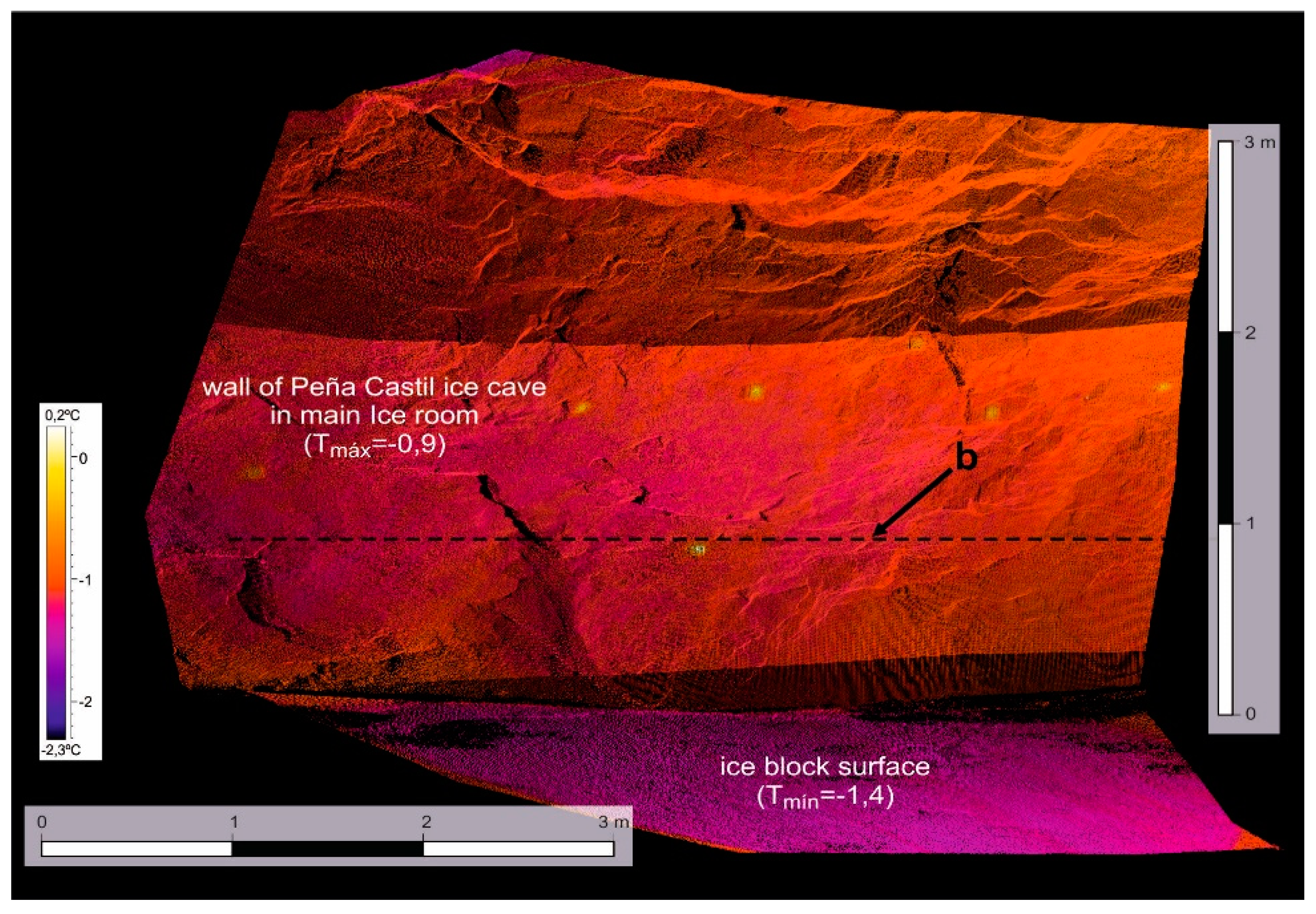
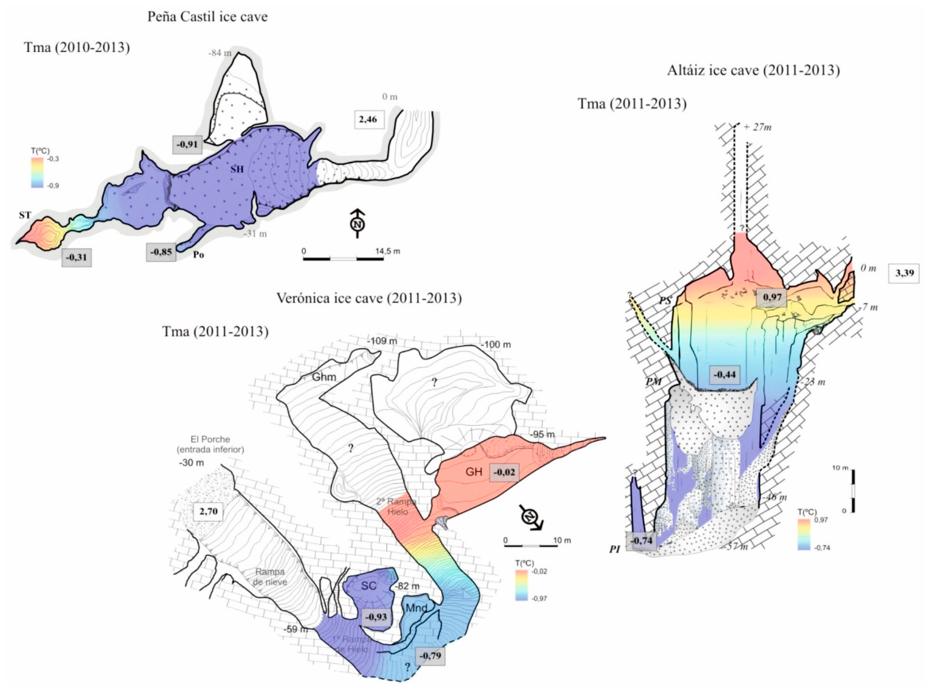
Figure 18.
Some Mean Annual Air Temperatures maps in Picos de Europa ice caves obtained by combining different method presented.
Figure 18.
Some Mean Annual Air Temperatures maps in Picos de Europa ice caves obtained by combining different method presented.

Figure 19.
Cryomporphological topography of Peña Castil ice cave.
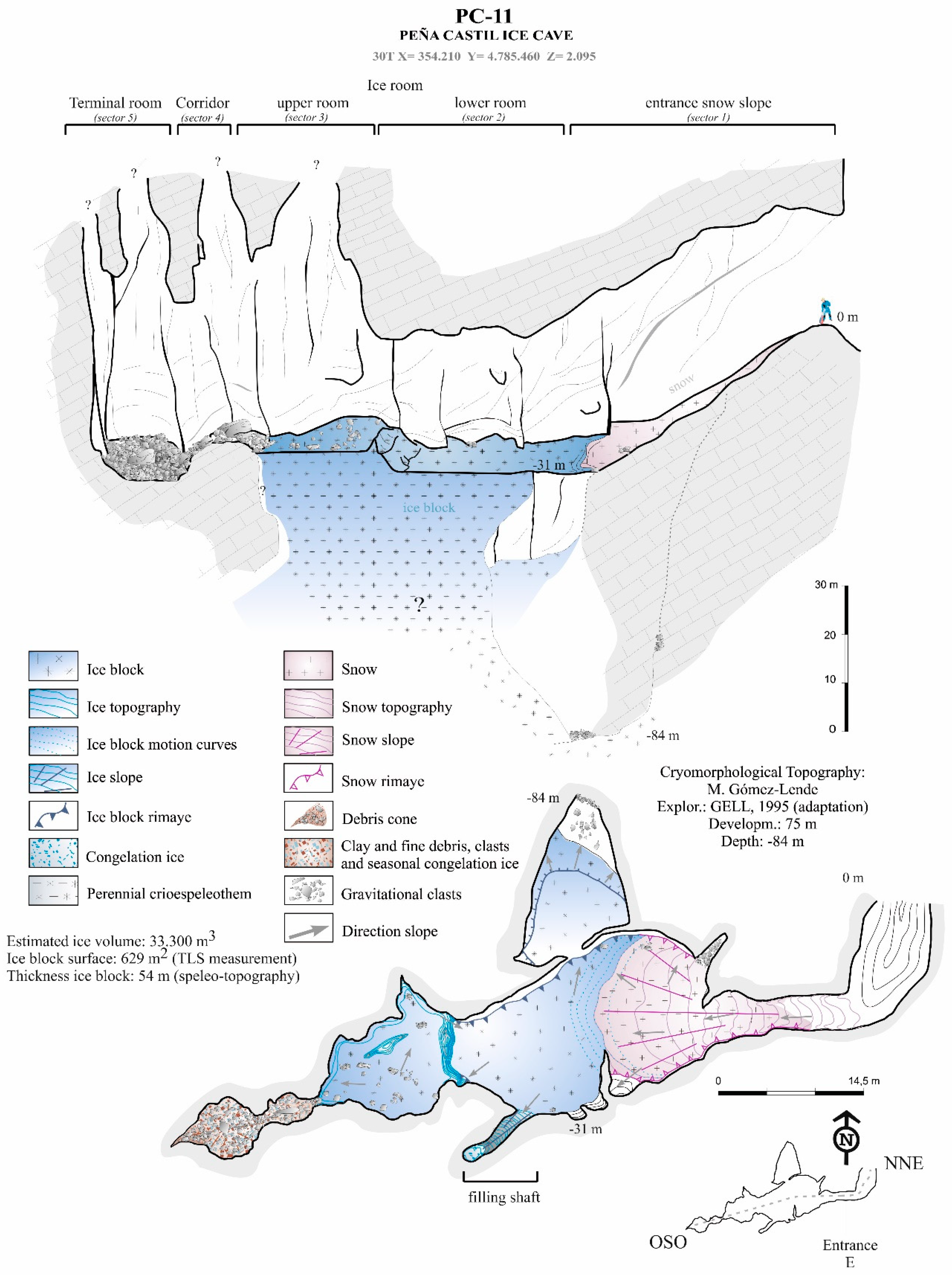
Figure 20.
Cryomporphological topography of Altáiz ice cave.
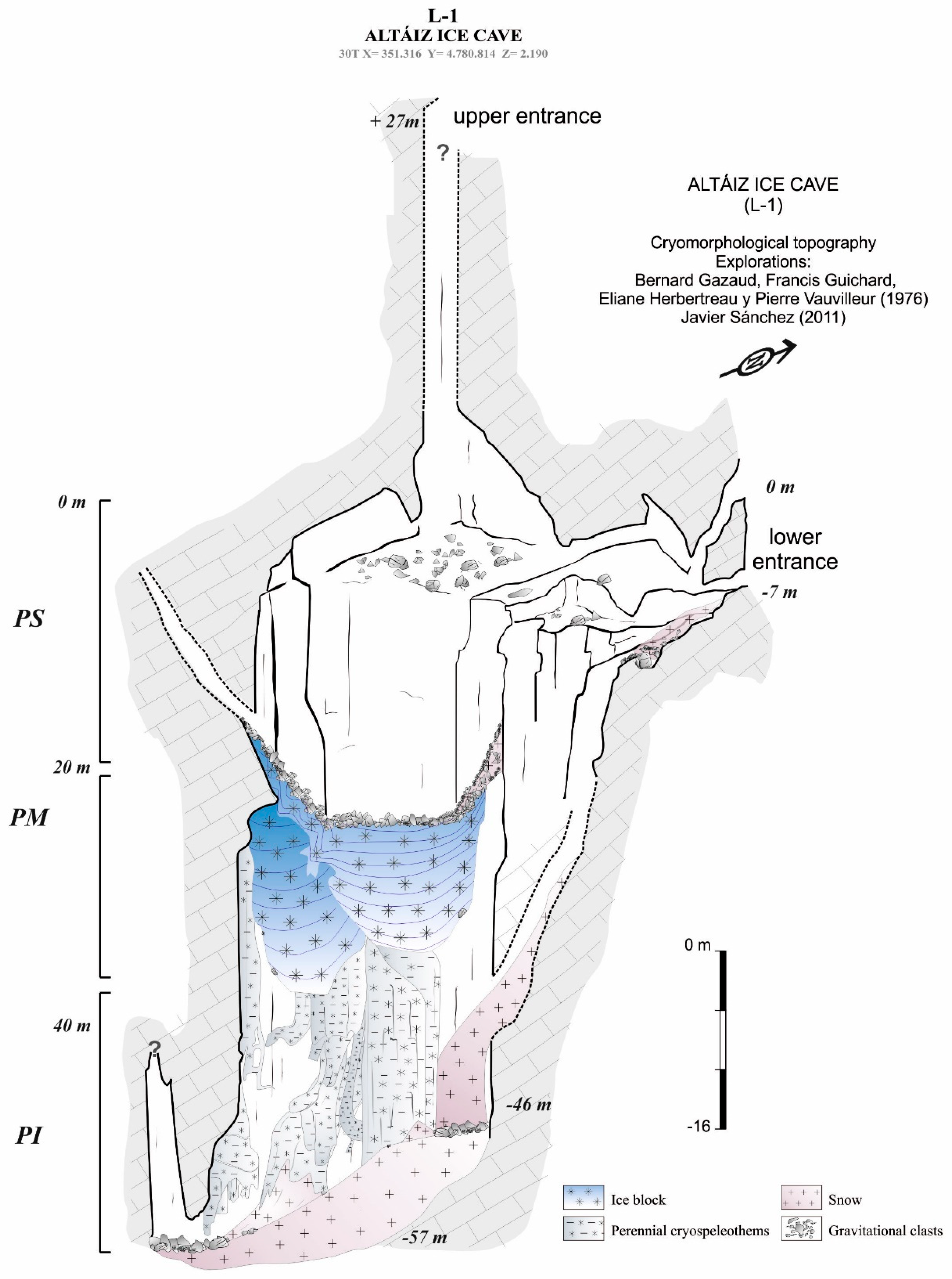
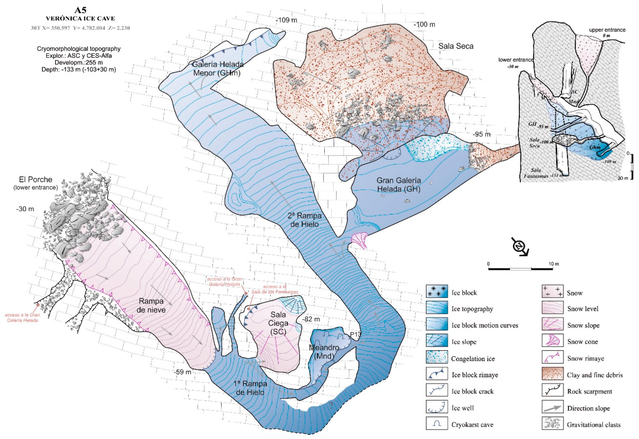
Figure 21.
Cryomporphological topography of Verónica ice cave.

Table 1.
Configuration parameters for the FARO equipment. In the case of reading with an image to take color at the time expressed, it would be necessary to add 3 more minutes in all cases.
Table 1.
Configuration parameters for the FARO equipment. In the case of reading with an image to take color at the time expressed, it would be necessary to add 3 more minutes in all cases.
| Resolution | Points Distance (mm/10 m) | Quality | Timing Scan (mm:ss) |
|---|---|---|---|
| 1/20 | 30.68 | 4x | 1:17 |
| 1/16 | 24.54 | 4x | 1:26 |
| 1/10 | 15.34 | 4x | 2:08 |
| 1/8 | 12.27 | 4x | 2:47 |
| 1/5 | 7.67 | 4x | 3:17 |
| 1/4 | 6.163 | 3x | 4:34 |
| 1/4 | 6.163 | 4x | 8:09 |
| 1/2 | 3.06 | 4x | 29:37 |
| 1/1 | 1.53 | 4x | 1 h 55 min |
Table 2.
Example of results of the point clouds union obtained with the FARO TLS.
| Cluster | Overlap (%) | Mean Precision (mm) | N Used Ptos. | % Ptos with <4 mm Precision |
|---|---|---|---|---|
| 3 northern takes | 76.3 | 2.15 | 237.487 | 72.6 |
| 2 central takes | 73.4 | 6.03 | 65.785 | 62.2 |
| 6 southern takes | 67.3 | 4.22 | 487.248 | 59.5 |
| Ice cave | 34.9 | 6.77 | 36.805 | 30.8 |
© 2018 by the authors. Licensee MDPI, Basel, Switzerland. This article is an open access article distributed under the terms and conditions of the Creative Commons Attribution (CC BY) license (http://creativecommons.org/licenses/by/4.0/).
Share and Cite
MDPI and ACS Style
Gómez-Lende, M.; Sánchez-Fernández, M. Cryomorphological Topographies in the Study of Ice Caves. Geosciences 2018, 8, 274. https://doi.org/10.3390/geosciences8080274
AMA Style
Gómez-Lende M, Sánchez-Fernández M. Cryomorphological Topographies in the Study of Ice Caves. Geosciences. 2018; 8(8):274. https://doi.org/10.3390/geosciences8080274
Chicago/Turabian StyleGómez-Lende, Manuel, and Manuel Sánchez-Fernández. 2018. "Cryomorphological Topographies in the Study of Ice Caves" Geosciences 8, no. 8: 274. https://doi.org/10.3390/geosciences8080274
Note that from the first issue of 2016, this journal uses article numbers instead of page numbers. See further details here.