Lithosphere–Atmosphere–Ionosphere Coupling Effects Based on Multiparameter Precursor Observations for February–March 2021 Earthquakes (M~7) in the Offshore of Tohoku Area of Japan

Abstract

The purpose of this paper is to discuss the lithosphere–atmosphere–ionosphere coupling (LAIC) effects with the use of multiparameter precursor observations for two successive Japanese earthquakes (EQs) (with a magnitude of around 7) in February and March 2021, respectively, considering a seemingly significant difference in seismological and geological hypocenter conditions for those EQs. The second March EQ is very similar to the famous 2011 Tohoku EQ in the sense that those EQs took place at the seabed of the subducting plate, while the first February EQ happened within the subducting plate, not at the seabed. Multiparameter observation is a powerful tool for the study of the LAIC process, and we studied the following observables over a 3-month period (January to March): (i) ULF data (lithospheric radiation and ULF depression phenomenon); (ii) ULF/ELF atmospheric electromagnetic radiation; (iii) atmospheric gravity wave (AGW) activity in the stratosphere, extracted from satellite temperature data; (iv) subionospheric VLF/LF propagation data; and (v) GPS TECs (total electron contents). In contrast to our initial expectation of different responses of anomalies to the two EQs, we found no such conspicuous differences of electromagnetic anomalies between the two EQs, but showed quite similar anomaly responses for the two EQs. It is definite that atmospheric ULF/ELF radiation and ULF depression as lower ionospheric perturbation are most likely signatures of precursors to both EQs, and most importantly, all electromagnetic anomalies are concentrated in the period of about 1 week–9 days before the EQ to the EQ day. There seems to exist a chain of LAIC process (cause-and-effect relationship) for the first EQ, while all of the observed anomalies seem to occur nearly synchronously in time for the send EQ. Even though we tried to discuss possible LAIC channels, we cannot come to any definite conclusion about which coupling channel is plausible for each EQ.

1. Introduction

Short-term earthquake (EQ) prediction is of vital importance for human beings to mitigate natural disasters [1]. During the last few decades, precursory phenomena of EQs have been extensively investigated for EQ prediction, and many papers have been published on various kinds of nonseismic, especially electromagnetic, precursors. Among many precursors, we can list some early days’ convincing case studies on ULF (ultralow frequency) lithospheric radiation for huge EQs, including the 1988 Spitak EQ [2,3], the 1989 Loma Prieta EQ [4], and the 1993 Guam EQ [5], and also on the ionospheric perturbations for the 1995 Kobe EQ with the use of subionospheric VLF (very low frequency)/LF (low frequency) waves [6]. Then, accumulation of a lot of case studies for huge EQs, such as the 1999 Chi-Chi EQ, the 2004 Sumatra EQ, the 2008 Wenchuan EQ, and the 2011 Japan EQ, led us to believe that there appear definitely electromagnetic precursors as possible candidates for short-term EQ prediction (e.g., [1,7,8,9,10,11]). This conclusion has been recently well evidenced by further statistical studies for various precursors in different regions of the earth, for example, DC and ULF lithospheric radiation (e.g., [12,13]), different atmospheric parameters as mainly observed from space (e.g., [14,15]), and ionospheric perturbations both in the lower part [16,17,18] and in the upper F region (e.g., [19,20]). These papers succeeded in showing the significant correlation of each effect with EQs, but it is needless to say that further studies are highly required for other phenomena based on long-term observational data. Moreover, it has been established by a huge amount of subionospheric VLF/LF observation (e.g., [16,17,21,22,23,24,25]), ionosonde observation, satellite-based GPS (global positioning system) TEC (total electron content) observation (e.g., [26,27]), and in situ satellite plasma and wave observations [10,28] that the ionosphere is extremely sensitive to preseismic lithospheric activity, and it is suggested as the most promising candidate for short-term EQ prediction (e.g., [29,30]), even though the mechanism of why and how the ionosphere is perturbed as the influence of lithospheric activity is controversial. Therefore, the recent greatest concern of our seismo-electromagnetic studies is elucidation of the mechanism of lithosphere–atmosphere–ionosphere coupling (LAIC) (e.g., [7,8,10,11,31,32,33,34,35]). For the study of the LAIC process, the multiparameter observation is highly recommended (e.g., [11]), that is, a combined study of different parameters of lithospheric, atmospheric, and ionospheric perturbations with the full use of ground- and satellite-based observational data (see, e.g., [36,37]). In addition to those short-term precursors, there have been observed a few imminent (lead time of less than 1 day) precursors [8], including the recent GPS TEC ionospheric perturbation [38].

Another important direction we are pursuing in recent years is the application of critical analysis of various seismo-electromagnetic phenomena in order to understand what is happening in each region of the LAIC process (e.g., [39,40,41,42,43,44,45]); that is, we can study the nonlinear self-organized criticality process especially in the lithosphere and the neighboring regions. This study will surely reinforce the above statistical analyses in the sense that we can understand whether an anomaly is at the critical stage of pre-EQ lithosphere or not. However, no such critical analysis is treated in this paper.

Here, the mechanism of the LAIC process has been studied extensively for the last 10 years, and a few hypotheses have already been proposed (e.g., [7,8,10,31,32,35]). As is given in Hayakawa et al. (2004) [32], the first is so-called chemical channel, in which emanation of radioactive radon and/or gases is considered to play the main player, leading to the modification of atmospheric conductivity and generation of electric field, thereby driving a variation in the ionospheric plasma density [7,28,35,46,47,48,49]. The second is acoustic channel, in which atmospheric oscillations, including atmospheric gravity waves (AGWs) and acoustic wave, are excited by the precursory deformation of ground motion and/or gas emanation [8,33,50,51,52,53], propagating upwards to the lower and upper ionosphere and leading to a perturbation in the ionosphere [54,55,56,57]. The third is electromagnetic channel [32], where electromagnetic waves generated in any frequency range propagate upwards into the ionosphere and magnetosphere, inducing the particle precipitation into the upper atmosphere due to wave–particle interactions in the magnetosphere (e.g., [58,59,60,61]). Finally, a fourth electrostatic channel is proposed based on the laboratory experiments, in which positive holes are generated when the ground of our interest is stressed by the accumulated pressure [62]. These processes have been discussed extensively by different authors (e.g., [11]), but any of the above hypotheses has not been evidenced by any observational data, requiring further studies until the process of LAIC is well understood. In [62], they tried to interpret various observables in the context of positive hole hypothesis. Many papers using subionospheric sounding with the VLF/LF technique have been published, providing a lot of indirect evidence on the AGW hypothesis [21,22,51,52,63,64,65,66,67], but recent studies on the AGW activity in the stratosphere have given convincing direct support to this AGW hypothesis [53,54,55,56,57].

The purpose of this paper is to try to have a better understanding of the LAIC mechanism by dealing with two successive major EQs with different seismological hypocenter conditions that happened recently in Japan in February and March 2021 in the offshore of the Tohoku area of Japan island. Those EQs had a nearly equal magnitude of M~7 and happened nearly at similar epicenters, but we feel that the hypocenter conditions are significantly different from each other in the sense that the first EQ happened within the subducting plate, while the second EQ happened at the seabed of the subducting plate just like the disastrous 2011 Tohoku EQ. Therefore, by considering this geological and seismological difference between these EQs, we expect significant morphological differences in the LAIC process for those two EQs, such as the emanation of radioactive radon and/or gases, excitation of AGWs, and so on. With this expectation, we will attempt to perform multiparameter analyses to compare the characteristics of different seismogenic precursors of the atmospheric and ionospheric perturbations for these EQs in order to find out whether there exists any significant difference between these EQs or not. The data used are ULF magnetic fields observed at Kakioka (KAK), Japan, in order to study the lithospheric radiation and lower ionospheric perturbations; ULF/ELF electromagnetic data from the network observation of Chubu University to study the atmospheric ULF/ELF radiation; stratospheric AGW activity data from the temperature data from a satellite; subionospheric VLF/LF propagation data observed in Kamchatka, Russia; and GIM (global ionosphere map) TEC (total electron contents) ionospheric data for the upper ionospheric perturbations. The period of analysis of all observables is 3 months from the beginning of January to the end of March (sometimes several days in April). The main results of this paper based on the analyses over the whole period are that all of the electromagnetic anomalies in different regions of the lithosphere, atmosphere, and ionosphere appeared only in a period from about 1 week to the EQ days (but sometimes even after the EQ day), and we try to interpret those anomalies in the context of the LAIC process.

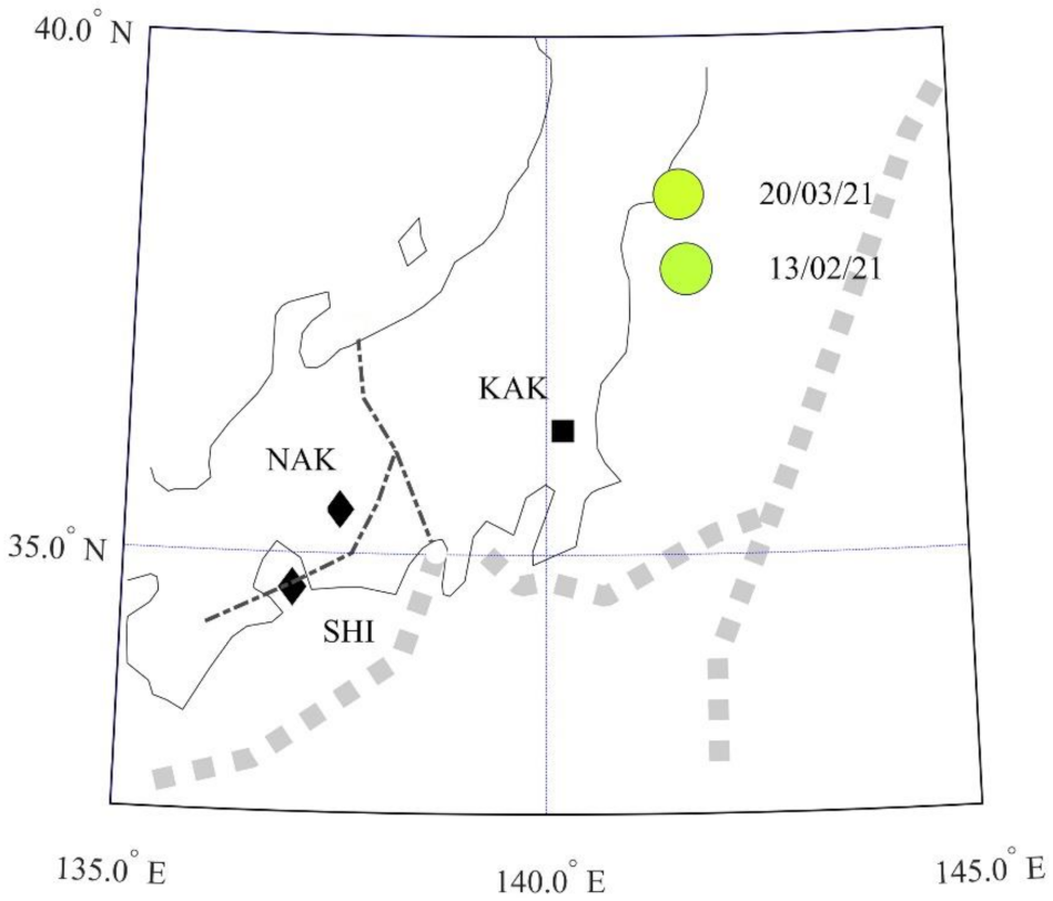
2. Two EQs Used in This Paper

It seems that this year we noticed a significant enhancement of seismic activity especially in the Pacific Ocean side of Japan island, probably as aftershocks of the disastrous 2011 Tohoku EQ in the seismological sense. There happened two successive huge EQs in the Tohoku offshore area in February and March 2021, which will be our target.

The first EQ (called Fukushima-ken-oki EQ) took place at 23 h 7 min on 13 February 2021 (LT) (or UT = 14 h 7 min on 13 February) with a magnitude of M = 7.3 and with a depth of 55 km. Its epicenter is at the geographic coordinates of 37.7° N, 141.7° E. The second EQ (called Miyagi-ken-oki EQ) happened at 18 h 9 min on 20 March 2021(LT) (UT = 9 h 9 min on 20 March) at its epicenter located at 38.5° N, 141.6° E with a magnitude of M = 6.9 and a depth of 59 km. These EQs are plotted in Figure 1, together with the Kakioka (KAK) ULF station and two stations (Nakatsugawa (NAK) and Shinojima (SHI)) of the Chubu University ULF/ELF network.

These doublet EQs are quite similar to each other because of a nearly equal magnitude of around 7, a depth of about 60 km, and being in close vicinity (with the separation of about 100 km), but we want to emphasize a significant difference in the geological and seismological conditions of these EQ hypocenters with special reference to the LAIC process. The second EQ is found to be quite similar to the famous disastrous 2011 Tohoku EQ in the seismological sense that this EQ happened at the seabed or the upper surface of the subducting Pacific Ocean plate and at the border between the Pacific Ocean plate and the land plate, leading to a possibility of inducing a tsunami. On the other hand, the first EQ took place as a rupture within the subducting Pacific Ocean plate (or within the slab), not at the seabed. This may look just a minor effect, but we want to pay great attention to this difference in EQ hypocenter condition with respect to the plate, and we would like to try to look into whether there is any remarkable difference in the morphological characteristics of observed precursory atmospheric and ionospheric perturbations, leading to better understanding of the LAIC mechanism.

We use the local seismicity at an observing station by an index K_LS:

$$K_{LS}=\frac{{10}^{0.75M}}{10(R+100)}$$

(1)

where R is the distance from the observation station to the EQ epicenter (in km) and M is the local EQ magnitude. Molchanov and Hayakawa (2008) [8] introduced a similar index to study seismoacoustic emissions. In this index, they took into account the attenuation of seismic waves in the earth’s crust, even though low frequency waves propagate in the earth–ionosphere waveguide with very small damping.

According to the formulas [68,69], the size (or radius) of the EQ preparation zone is estimated to be about 1000 km so that the observatory of KAK and also the two stations of NAK and SHI are well within the radius of this EQ preparation zone.

Further, it is very important to note whether any anomaly is related to any space weather perturbations (solar activity, geomagnetic activity, and so forth), so we used the conventional geomagnetic activity index, Dst, and Kp index taken from World Data Center at Kyoto. Sometimes we use the solar activity expressed by F10.7.

3. Multiparameter Observational Data and Analysis Methodology

3.1. ULF/ELF Data

We use the ULF magnetic field data observed at the Kakioka Magnetic Observatory belonging to Japan Meteorological Agency (JMA) (geographic coordinates: 36.23° N, 140.18° E). One-second sampling ULF data observed by a fluxgate magnetometer are available for our study, and two magnetic field components (H and Z) are analyzed.

Then we use the ULF/ELF electromagnetic field data observed by the network of Chubu University, which is composed of three observing stations: Nakatsugawa (NAK, 35.42° N, 137.55° E), Shinojima (SHI, 34.67° N, 137.01° E), and Izu (IZU, 34.64° N, 138.85° E). Unfortunately, the equipment at IZU was not working during our period, and so the data only from two stations of NAK and SHI plotted in Figure 1 are utilized. At each station, we measure the magnetic field changes (H, D, and Z) by means of three orthogonal magnetometers with 100 Hz sampling. The magnetometer is an induction coil sensor, and the details of the equipment are given in Ohta et al. (2013) [70]. The observed data are regularly transferred to the master station in Kasugai (Chubu University).

3.2. Analysis Methodology of ULF Data

3.2.1. Lithospheric ULF Radiation

With the use of ULF magnetic field data, we can study initially the well-known electromagnetic radiation from the lithosphere as mentioned before (e.g., [2,3,4,5]), which has been extensively investigated recently all over the globe with a lot of attention [13,71,72].

After the FFT analysis of 1 s sampling ULF data at Kakioka, we estimate the power spectral densities of two magnetic field components, Fh, and Fz and also the polarization Pz/h [5] at different frequencies. The polarization is defined as the ratio of the power spectral densities of the vertical component to the horizontal component, and this parameter is found to effectively detect seismogenic ULF radiation [73,74].

3.2.2. ULF Magnetic Field Depression

Even with using the same ULF data, we can study a rather new topic of depression of ULF horizontal magnetic field initially discovered by Molchanov et al. (2014) [75,76,77,78,79], which is the depletion in the intensity of nighttime irregular pulsations from the magnetosphere. This effect is not so popular even in the academic society, but it is suggested by them that this effect is attributed to the lower ionospheric turbulences [76,77] just like the subionospheric VLF/LF perturbation [16,30]. We have to show the analysis method of ULF depression here. The value of absolute depression $De{p}_h$ in the horizontal component H of ULF magnetic field variations is calculated as:

$$De{p}_h=\frac{1}{{〈F_h{}^2〉}_{\Delta T}}$$

(2)

where in the denominator we have the squared output signal $F_h$ observed by the sensor in the frequency band of $\Delta$F = 0.01–0.02 Hz averaged over the local night interval $\Delta T$ = 01-05 JST(LT). As a measure of relative depression for the i-th date $\delta De{p}_{hi}$, we adopt the following value.

$$\delta De{p}_{hi}=\frac{De{p}_{hi}-\frac{1}{N}{\displaystyle \sum _{j=i-N}^{j=i-1}De{p}_{hj}}}{\frac{1}{N}{\displaystyle \sum _{j=i-N}^{j=i-1}De{p}_{hj}}}$$

(3)

Here, $De{p}_{hi}$ is the depression for the i-th date. N is the filter parameter equal to the number of preceding days for averaging, and in the present study, N = 7 is taken to reduce the effect of 1–few days’ changes in the variations of the magnetic field. Processing parameters (ΔF, ΔT and N) are determined experimentally from the properties of local interference and depression.

3.3. Analysis Method of ULF/ELF Electromagnetic Radiation

On the other hand, ULF/ELF electromagnetic radiation in the frequency range from 1 Hz to about 50 Hz is found to be an atmospheric phenomenon associated with EQs [78], whose possible mechanism is suggested to be due to the gas ejection from the lithosphere [80]. Even though a statistical study on this phenomenon was first published by Schekotov et al. (2007) [78], this effect is not so popular either in the academic society. However, recently, Fidani et al. (2020) [81] confirmed the presence of this ULF/ELF impulsive radiation with their Italian network and suggested it as a short-term EQ predictor, but unfortunately, they have not yet provided any statistical study as in [78,80,82,83].

Because this atmospheric ULF/ELF impulsive radiation is again not well known in the society, we will repeat the analysis (or detection) methodology here. The detection of atmospheric ULF/ELF electromagnetic radiation is composed of two processes, as shown below. The first is direction finding, and the second is the detection of ULF/ELF radiation.

3.3.1. Direction Finding

We determine the direction of the source of seismo-atmospheric ULF/ELF radiation as being perpendicular to the main axis of the polarization ellipse. We denote by θ the angle between the main axis of the polarization axis and the D (EW) component axis, and its tangent is given by the following equation [84].

$$\tan (2\theta )=\frac{2A_h{A}_d}{A_d^2-A_h^2}\cos \left({\varphi }_h-{\varphi }_d\right)$$

(4)

Here, $A_h$, $A_d$ and ${\varphi }_h$, ${\varphi }_d$ are instantaneous amplitudes and phases of the field component signals. h refers to the NS component of magnetic field, while d, the EW component. They are computed from appropriate complex signals, which are, in turn, obtained from the real signals (U_h and U_d) by means of the Hilbert transform. The last ones are extracted from the recorded signals with filtration in the band 10–12 Hz due to industrial noise at frequencies below the first Schumann resonance mode and thunderstorm interferences at Schumann resonance frequencies.

The angle θ in an interval (−π/2, π/2) is totally determined by Equation (4) and by the signs of the numerator and denominator of the right-hand side of Equation (4). This angle is connected with the azimuth angle (α) of the radiation source.

α = π − θ

(5)

It is determined in the interval of (3π/2, π/2). These same data α were added in the interval (π/2, 3π/2) to provide the determination of α in the whole interval of (0, 2π). The value of α(i) for i satisfied the following conditions:

$$\sqrt{\left(U_h^2(i)+U_d^2(i)\right)}>K\sqrt{〈U_h^2+U_d^2〉}$$

(6)

which were used to obtain the azimuth distribution. The notation < > on the right-hand side of Equation (6) means the average value of horizontal magnetic field. Here, i is an index of discrete values of the signal that obey Equation (6). Additionally, we adopt K = 3, which determines the maximal signal-to-noise ratio. The last condition of sufficient signal-to-noise ratio is of essential importance to provide the required accuracy of a direction finding.

Azimuthal distribution is laid over the map of the region shown in equidistant azimuthal projection. The distribution of α is represented by an angle histogram, which is a polar plot showing the distribution of α values. Each group in each polar plot is shown as one bin, and each polar plot shows α(i) in 72 angle bins, providing a resolution of 5°. The length of each lobe in the histogram and its degree of darkness are proportional to the number of elements in α(i) that fall within a bin. On the edge of the round panel, we have a ring on which the degree of blackness reflects the total azimuthal distribution of the last 6 days of observations. This “search light” indicates the most probable azimuths of ULF/ELF radiation and the corresponding plausible azimuths of a forthcoming EQ. They correspond to the darkest sectors of the ring.

3.3.2. Detection of the Radiation

In our previous paper by Schekotov et al. (2007) [78], we proposed a new parameter ∆S in order to detect seismo-atmospheric ULF/ELF radiation, which is given by:

$$\Delta S=\frac{\frac{P_{hh}}{P_{dd}}-1}{rms(\tan \beta )}$$

(7)

The numerator contains the ratio of two horizontal spectral components, P_hh (NS component of magnetic field) (corresponding to Ph in the ULF analysis) and P_dd (EW component) (Pd in the ULF analysis). The denominator is the root mean square (rms) of the deviation of the signal ellipticity. The expression of β is given by the following equation.

$$\beta =\frac{1}{2}\arcsin \left\{\frac{\mathrm{Im}(P_{dh}-P_{hd})}{{\left[{\left(P_{hh}-P_{dd}\right)}^2+4P_{hh}{P}_{dd}\right]}^{1/2}}\right\}$$

(8)

Here, Im means imaginary part. Schekotov et al. (2007) [78] compared different parameters and found an enhancement in the spectral ratio of P_hh/P_dd and a reduction in the polarization ellipticity before an EQ, and the parameter introduced by Equation (7) is proved to be most sensitive and reproducible to seismic shock [78,82,83]. The ellipticity or the ratio of minor axis to major axis is defined by tan β. The sense of polarization is characterized by the sign of β; when β > 0, the polarization is right-hand (RH), and β < 0 means left-hand (LH) polarization. The linear polarization is expressed by β = 0 [84].

The field component power spectral densities, P_hh and P_dd, and their cross-power spectral densities, P_hd and P_dh, were calculated by using Fourier transforms with a frequency resolution of about 0.1 Hz. Spectral components at a frequency range of 0.1 to 30 Hz were taken into account in this paper. They were averaged over 1 Hz intervals, such as 0.1–1, 1.1–2, …, 29.1–30 Hz, so that we have 30 spectral components in the present analysis.

The success in the application of this parameter ∆S was partly due to a random fact that a majority of nearby EQs took place east of Karymshiro, Kamchatka, Russia [78]. In a more general case with the rotation of axes by some angle $\phi$, we can find a maximum of ∆S ($\phi$_i). Its radial component will be directed to the source of radiation. The radial P_rr and tangential P_tt field components should be taken instead of P_dd and P_hh.

$$\Delta S=\max {\left.\left\{\frac{\frac{P_{tt}\left({\phi }_i,f,t\right)}{P_{rr}\left({\phi }_i,f,t\right)}}{rms\left(\tan \beta \left(f,t\right)\right)}\right.\right\}}_{t,\phi ,f}$$

(9)

$${\phi }_i=0:\Delta \phi :\left(\pi -\Delta \phi \right)$$

where $\phi$_i is the angle of rotation, ∆$\phi$ is a step of rotation angle (10° in our case), and P_tt and P_rr are the tangential and radial component power spectral densities of the field, calculated from the elements of a coherency matrix by means of the following transformation.

$$\begin{array}{l}{P}_{tt}=P_{hh}{\cos }^2\phi +P_{dd}{\sin }^2\phi +\mathrm{Re}(P_{hd})\sin 2\phi \\ P_{rr}=P_{hh}{\sin }^2\phi +P_{dd}{\cos }^2\phi -\mathrm{Re}(P_{hd})\sin 2\phi \end{array}$$

(10)

Here, we repeat the physical significance of Equations (7) and (8), which consists in using two characteristics of the signal to improve the detection of seismogenic ULF/ELF radio emissions. The meaning of the numerator in Equation (9) consists in obtaining the maximum ratio of signal components for a given direction of the source. A small deviation of the signal ellipticity results in a decrease in the denominator in the presence of the signal. Both of these factors might lead to a growth of ∆S in the presence of the signal and consequently facilitate its detection. Next, we find the frequency and time interval where ∆S has maximal value.

3.4. AGW Activity Data

AGW activity in the stratosphere possibly triggered by EQs has been studied in our previous papers [53,54], in which ERA5 reanalysis data have been used to investigate the vertical (altitudinal) perturbations of temperature vertical (height) profiles for the study of AGW activities. In this paper, we use the same dataset and method, as used in our previous papers [53,54], to evaluate AGW activities around the EQ epicenters to see whether the stratosphere was perturbed or not before these two huge EQs in 2021.

ERA5 is a reanalysis dataset produced by the European Centre for Medium-Range Weather Forecasts (ECMWF), providing numerous atmospheric, land, and oceanic variables. Many kinds of observations include satellites, radiosondes, radars, and air-based and ground-based in situ measurements, which are assimilated into ECMWF’s meteorological forecast model [85]. ERA5 provides hourly temperature profiles covering the globe with ~31 km horizontal resolution from January 1950 to the present. ERA5 data are available from near the surface to 0.01 hPa (~80 km altitude) with 137 model levels in the vertical direction. However, we only focus on the stratosphere (around 15–50 km altitude) in this paper because evident anomalies on AGW activity were found in the stratosphere in our previous EQs [53,54]. On the other hand, ERA5 provides global temperature profiles, and so the data not only at the two EQ epicenters but also in the neighborhood of Japan are taken to investigate AGW activity in this paper. The particular region being taken is longitude from 110° E to 160° E and latitude from 20° N to 60° N.

Here, we have to describe the potential energy Ep as a representative of AGW activity in the stratosphere ([53,54] and references therein).

$$\mathit{Ep}=(1/2) (g/N{)}^2 (T/\overline{T}{)}^2$$

(11)

where g is the gravitational acceleration, N is the Brunt–Vaisala frequency that can be derived from atmospheric temperature T, and T′ is the fluctuation in temperature with respect to the background temperature $\overline{T}$. Both T and Ep are functions of latitude, longitude, altitude, and time. AGW activity is presumed to be triggered around the ground surface or lower atmosphere and further propagate into the upper atmosphere in the vertical direction. For evaluating AGW activity at the EQ epicenter, the vertical temperature profile there at a specific time is retrieved from ERA5, and a 2–10 km band-stop filter is used to filter out the wave components from T to establish $\overline{T}$. T′ is the difference between T and $\overline{T}$ (i.e., T′ = T − $\overline{T}$). The variance term (T′/$\overline{T})$², acting as the moving average of Ep, is calculated within a 2 km layer. A vertical profile of Ep is so evaluated. The same procedure is repeated numerous times until all the Ep values in the region of 110–160° E and 20–60° N are evaluated.

3.5. Subionospheric VLF/LF Propagation Data and Analysis

The lower ionosphere can be effectively monitored by subionospheric VLF/LF propagation, in which signals from VLF/LF transmitters propagate in the earth–ionosphere waveguide. Therefore, any space weather perturbations, such as the effects of geomagnetic storms, can be detected as a perturbation in VLF/LF data [86,87], and Hayakawa et al. (1996) [6] found convincing evidence of ionospheric perturbations prior to the 1995 Kobe EQ. Since then, a lot of attention has been paid to the use of subionospheric VLF/LF signals for seismo-ionospheric disturbance studies [18,21,22,23,24,25].

Russian colleagues [88] have established an observing station at Petropavlovsk (PTK), Kamchatka, Russia (53.09° N, 158.55° E), where the electric field of subionospheric VLF/LF signals in the frequency range of 10 to 50 kHz is detected by a VLF/LF receiver and the associated software, and both the amplitude and phase of transmitter signals are measured. The target transmitters treated in this paper are (1) JJY (Fukushima. f = 40 kHz), (2) JJI (Miyazaki in Kyushu, f = 22.2 kHz), and if necessary, (3) NWC (Australia, f = 19.8 kHz). Figure 2 illustrates the locations of the observing station, PTK, Russia, and two Japanese transmitters, JJY and JJI, as red triangles, together with their wave sensitive (or Fresnel) zones for each propagation path. Unfortunately, the transmitter of NWC is well outside of the figure, but you can find its Fresnel zone.

3.6. GIM TEC Data

Finally, we move on to the behavior at a higher altitude of the ionospheric F region. As introduced in Section 1, precursory perturbations have been found in the upper F region before many EQs (e.g., [19,20]). Those anomalies usually exist on the maximum electron density in the F2 layer (NmF2, or its corresponding plasma frequency, foF2), which is observed using ionosondes. However, an ionosonde can only observe the ionosphere above it, so not much spatial (horizontal) information is available using this kind of observation.

In the last two decades, scientists tried to use GPS/GNSS (global navigation satellite system) signals to derive TEC, which is highly correlated with the electron density in the F region. With the dense network of GPS/GNSS receivers around the globe, nowadays, it is possible to obtain a global view of TEC, and these TEC data are reliable and easy to obtain from a public dataset. In this study, we use TEC data from the GIM produced by CODE (Center for Orbit Determination in Europe, Bern, Switzerland). CODE GIM is constructed from GNSS signals observed by receivers around the world (see detailed information on this dataset in [89]). Its spatial resolution is 5 degrees in longitude and 2.5 degrees in latitude, and its temporal resolution is 1 h.

The TEC time series at the two EQ epicenters are retrieved from CODE GIM. Then we further compare the TEC values with their moving averages, which are constructed using the past 15-day values of the relevant day, to see whether the upper ionosphere was anomalously deviated or not before the two EQs.

4. Observational Results

4.1. ULF Magnetic Field (Lithospheric Radiation, ULF Depression)

Figure 3 illustrates the plots of ULF analysis results during 3 months from the beginning of January to the end of March 2021. The top panel shows the evolutions of geomagnetic activity of Kp (in blue) and local seismicity at Kakioka (Kls) (in yellow star). The second and third panels refer to Fh and Fz, respectively, and the fourth panel refers to the polarization Pz/h. The bottom two panels are the results of magnetic field depression, Dep and ΔDep, respectively. Vertical red broken lines indicate the occurrence times of two EQs. First of all, this figure suggests that there is a peak 4–5 days before the second EQ for both h and z components, which may be lithospheric radiation, but the polarization Pz/h is not significant on this day. Therefore, we have to say that the presence of ULF radiation is not so convincing. No clear ULF radiation is detected before the first EQ. Former works based on many case studies indicate that epicentral distances of 250–300 km are too far to observe such lithospheric radiation [5,72].

On the other hand, two peaks of ULF depression (i.e., variations in the bottom two panels and the corresponding peak in Pz/h) are very visible prior to two most powerful EQs. The dates of ULF depression are 11 February, 2 days before the first EQ, and 11 March, 9 days before the second EQ. The latter is also caused by the depression of the horizontal magnetic field component. The ULF depression is known to exhibit high sensitivity even for farther EQs, as is shown in [82], which is indicative of the appearance of lower ionospheric perturbations for both EQs. Of course, we do not know the positions of those ionospheric perturbations, which will be studied later with the use of AGW and TEC studies.

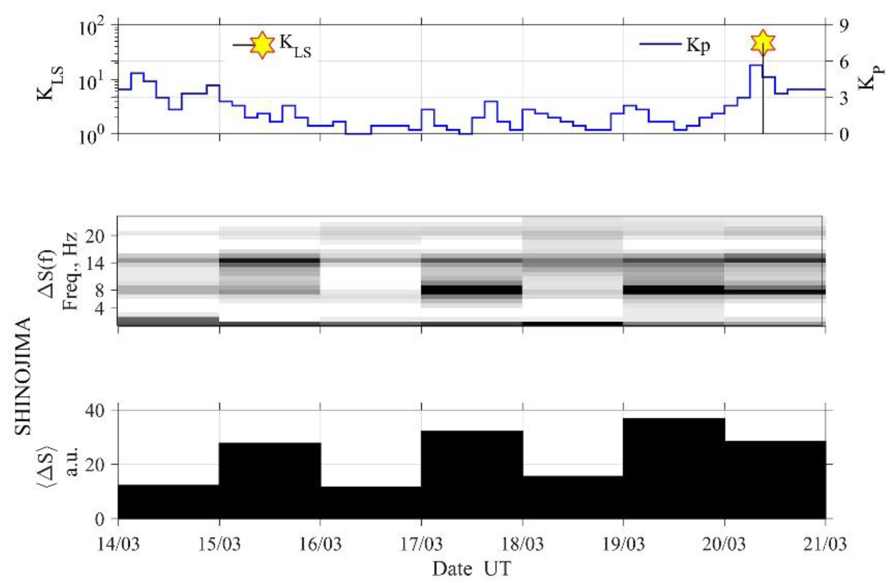
4.2. ULF/ELF Atmospheric Radiation

4.2.1. ULF/ELF Radiation Detection

We use ∆S in Equation (7) to detect ULF/ELF radiation, and Figure 4 demonstrates this radiation for the first February EQ. After having examined the data in January and February, we detected the radiation only during the period in Figure 4. The top panel as before illustrates evolutions of seismicity $K_{LS}$ and geomagnetic activity Kp. The next two panels display the spectrum of ΔS and its maximum values as observed in NAK only over the interval of 7–14 February 2021 when we observed ULF/ELF impulsive radiation. Two bottom panels display the corresponding spectrum and its maximum values observed in SHI over the same interval. The growth of the maximum values is observed at the frequencies of Schumann resonances starting 9 February to the EQ day (even after the EQ day). Perhaps this is due to the rise in the spectrum due to broadband ULF/ELF radiation as an EQ precursor.

Figure 5 illustrates the same signal characteristics as in the previous figure, but only for the interval from 14 March to 20 March 2021, as obtained in SHI for the second March EQ. Only during this interval we succeeded in detecting ULF/ELF radiation. Similar to the case of Figure 4, we can notice that this ULF/ELF radiation starts to be observed from 15 March till the occurrence of the second EQ.

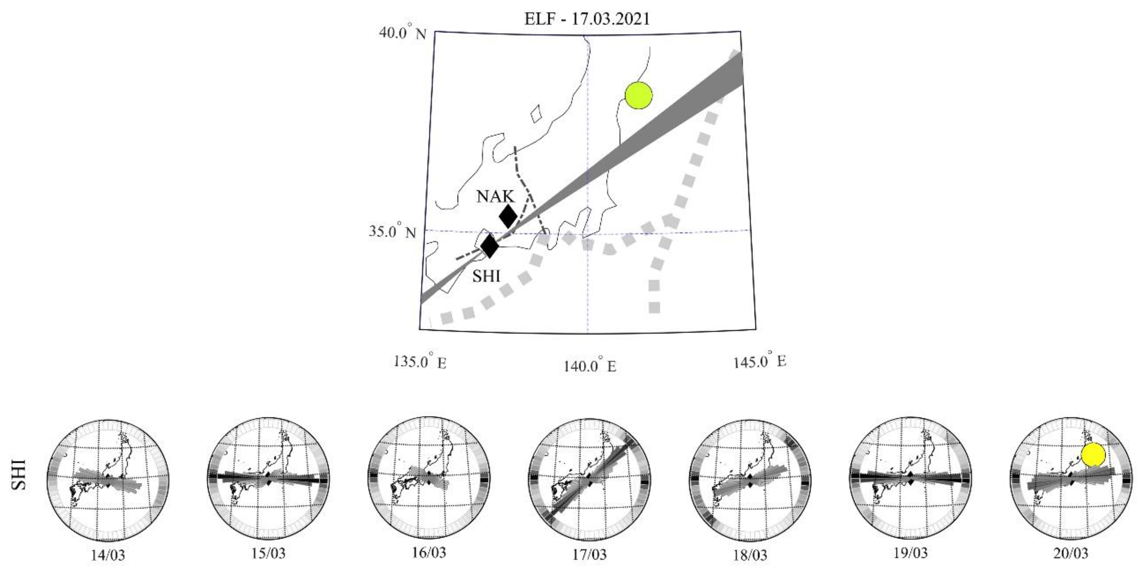
4.2.2. ULF/ELF Radiation Source Azimuth

After confirming the occurrence of seismogenic atmospheric ULF/ELF radiation, we will present the results of direction findings. Two rows of round panels of Figure 6 demonstrate the evolution of the azimuth distribution of ULF/ELF radiation for the first EQ on 7–12 February 2021 observed in NAK and SHI. At least during 3 days (9, 11, and 12 February), this radiation comes in from the upcoming EQ region. The three upper panels are found to confirm this fact. They show a map of the area, the position of the magnetometers, and the EQ that occurred on 13 February. Only the main lobes of the azimuthal distributions are illustrated here. Their cross section seems to lie anywhere between the coast and the Japan Trench.

On the other hand, seven round panels in Figure 7 illustrate the corresponding evolution of the azimuthal distribution of ULF/ELF radiation for the second EQ on 14–20 March 2021, as observed in SHI. No NAK data are available for this interval. The upper panel shows the position of the main lobe of the azimuthal distribution crossing the Japan Trench opposite to the epicenter of the upcoming EQ.

As the conclusion of the comparison of characteristics for the two EQs, we found that we could regularly observe the atmospheric ULF/ELF radiation for both EQs, suggesting no significant difference between the two EQs.

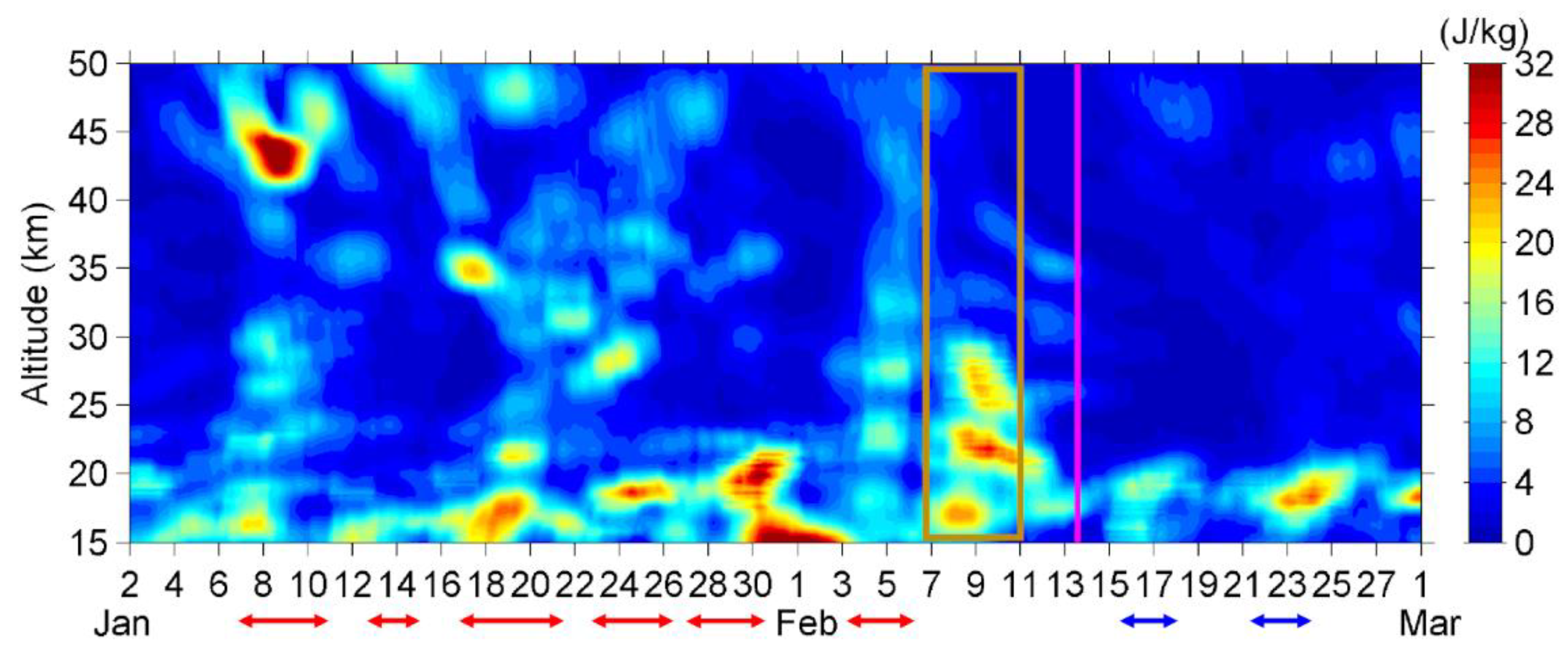
4.3. Observational Results on AGW Activity

Figure 8 illustrates the AGW activity result for the first February EQ, in which the potential energy Ep over the EQ epicenter is plotted as a function of altitude from 15 to 50 km. This figure indicates that AGW activity was very active in the stratosphere in January and early February before the first EQ. Because weather systems are the main sources of AGW activity in the stratosphere, we further check the weather maps and ground-based observations around the Tohoku region issued by JMA to eliminate the wave activities excited by weather systems. We found that most of these AGW activities in Figure 8 are likely to be attributed to winter weather systems in the relevant region. The red arrows at the bottom of the figure are due to the occurrences of some fronts and cyclones passing over the EQ epicenter after checking the weather maps. However, the AGW activity was also enhanced on 7–11 February (brown rectangle in the figure) (6 to 2 days before the first February EQ), and this enhancement was not related to any weather disturbance. Figure 9 and Figure 10 show the spatial distribution of potential energy Ep maps at the specific altitude of 21 km on 7 and 11 February, respectively. AGW was active around 40° N latitude on 7 February (Figure 9). However, a significant enhancement of wave activity was found to be located around the Tohoku offshore region, and the enhancement of Ep persisted for 5 days until 11 February (Figure 10). The enhanced area extended toward the northeast direction on 7 February, but it shrank gradually on the following days, and finally concentrated right above the EQ epicenter, covering a small part of the land. However, the enhancement always centered around the EQ epicenter on these days. Hence, these Ep enhancements of AGW activity could be a possible precursor to the first EQ on 13 February.

Besides, the AGW activity seems to be abnormal even after the EQ. There were two more frontal and cyclonic systems, as shown by the blue arrows in Figure 8, that influenced the Tohoku area around 15 February and 22–23 February based on the examination of weather maps. The one on 15 February was a very strong one. This cyclone developed quickly and experienced explosive cyclogenesis over eastern Japan, and its minimum surface pressure reached 946 hPa soon after it passed over the EQ epicenter. It is further considered as the strongest extratropical cyclone in January and February in the 2020–2021 winter that influenced Japan. In addition, thunderstorms were observed in some weather stations in Fukushima, Niigata, and Yamagata Prefectures (all are close to the EQ epicenter) when a cyclonic and frontal system passed over eastern Japan on 22–23 February, revealing that a convective weather system was active around the EQ epicenter during this period. Therefore, it is expected that AGW activity should be enhanced during the influence of these two systems. However, the AGW activity was enhanced only around the tropopause, but not propagated into the stratosphere, as seen in previous cases marked by the red arrows. This is very strange, making the AGW activity seem to be calm after the February EQ, but currently, we do not have enough evidence to identify whether this is a post-EQ or not.

How about the AGW activity for the second March EQ? Figure 11 is the corresponding result for the second March EQ. The same as in Figure 8, the red arrows in Figure 11 indicate the passing of some cyclonic and frontal systems over the EQ epicenter. Most of AGW activities during this period were excited by meteorological systems, although the Ep values during the influence of these systems are somewhat smaller than those in Figure 8. There are also two cases (blue arrows in Figure 11) regarding frontal systems that passed the EQ epicenter, but no considerable AGW activity is found in the stratosphere. It seems that no abnormal enhancement of Ep can be found in Figure 11. However, after checking all the Ep maps at each altitude, we noticed an interesting anomaly at 22 km altitude on 16–18 March, and Figure 12 and Figure 13 show the corresponding Ep maps on 16 and 17 March. A frontal system passed through the Korean Peninsula, Sea of Japan, Tohoku area, and the EQ epicenter on 16 March, and it should excite some AGW activities along its path. In Figure 11, it is seen that Ep was enhanced at an 18 km altitude on 16–17 March. From the Ep map on 16 March in Figure 12, it is also seen that AGWs were active around the area from the Korean Peninsula to Japan. The particular point we pay attention to is an enhancement of Ep, which is located around the EQ epicenter. This enhancement even intensified on 17 March in Figure 13, while the frontal system had already passed away and AGW activity became weaker in other areas. This enhancement of AGW activity decayed but still centered around the EQ epicenter on 18 March, and finally disappeared on 19 March (though figures are not shown). Although this enhancement at a 22 km altitude appearing 3–4 days before the second March EQ somewhat overlaps the influence of a frontal system, it still seems to be a possible preseismic effect, because it is located around the EQ epicenter and the Ep value there is higher than at other places where the frontal system influenced.

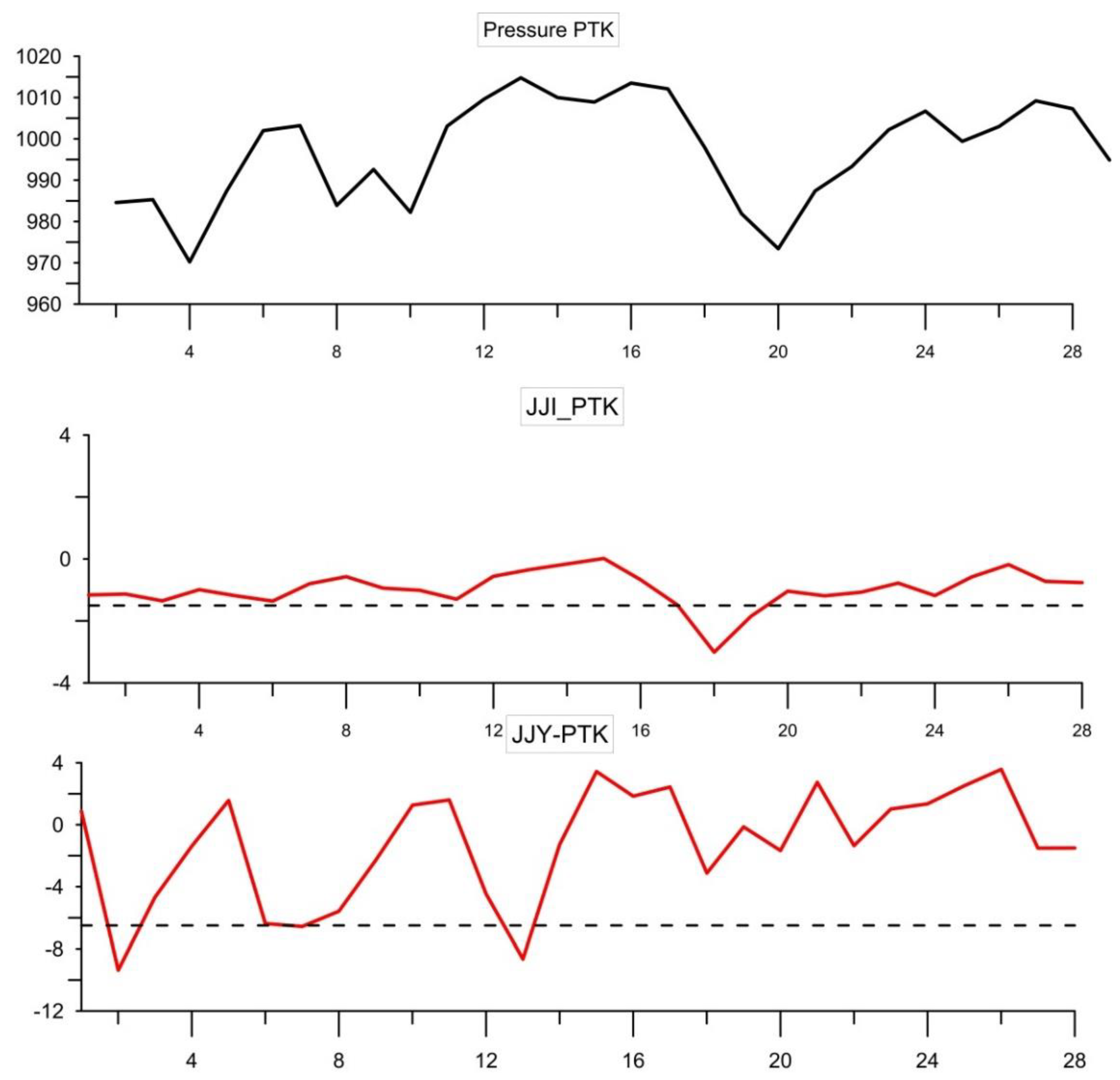
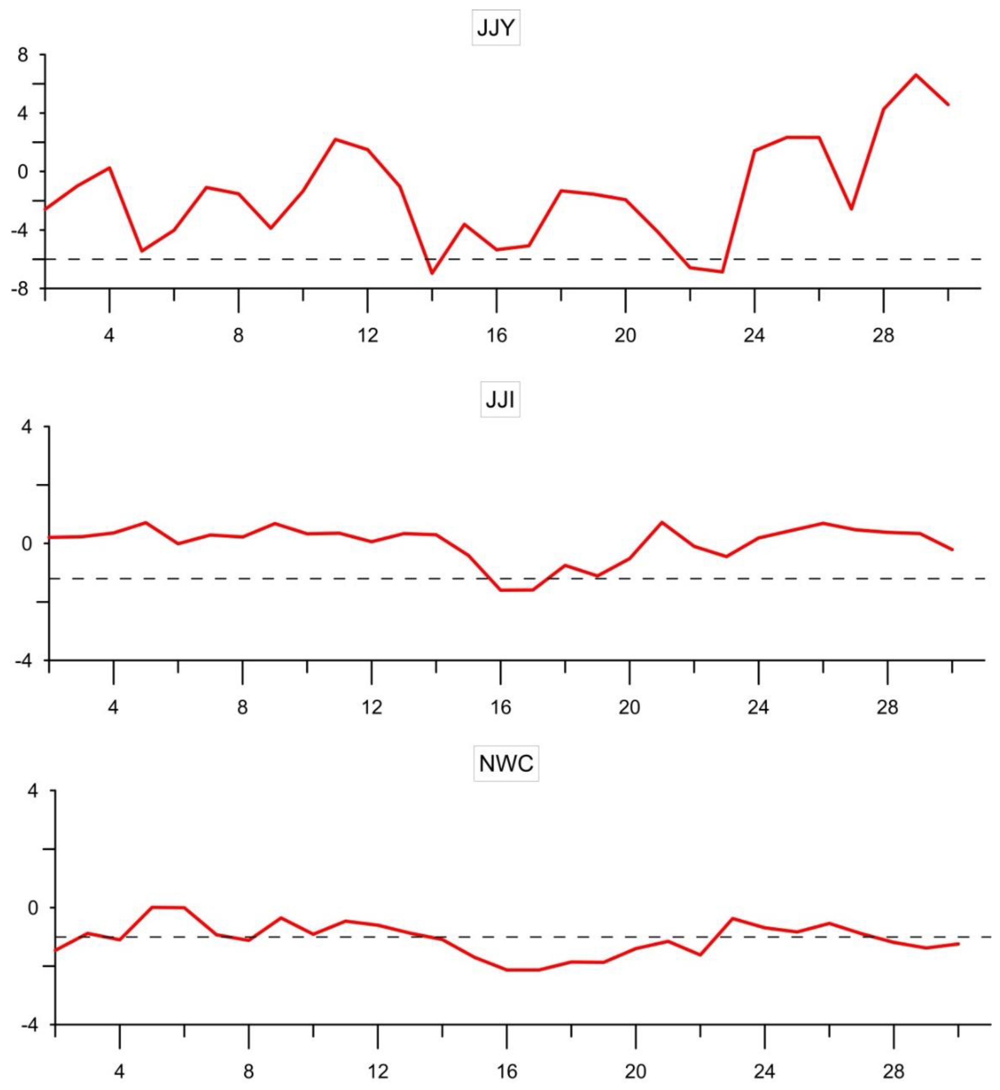
4.4. Subionospheric VLF/LF Propagation Anomalies (Lower Ionospheric Perturbations)

Subionospheric VLF/LF propagation results for the first EQ are presented in Figure 14, in which two propagation paths of JJY-PTK and JJI-PTK are shown. No anomaly was observed in January, so the result of February is shown in Figure 14. Here, we used the nighttime fluctuation method [16,21,22,23], where the abscissa indicates the day and the ordinate refers to the current nighttime amplitude (as an average of amplitude during the local night) in dB and the horizontal broken lines mean −2 sigma (sigma, standard deviation) for the detection of VLF/LF anomalies. For comparison, as the top panel we included the temporal change of atmospheric pressure at the station of PTK in order to eliminate the meteorological effects.

The temporal evolution of the nighttime amplitude of the path of JJI-PTK seems generally to be rather well correlated with the pressure variation, and a significant anomaly as depletion in nighttime amplitude is likely to be related to the pressure variation of meteorological effects.

In contrast to the path of JJI-PTK, the propagation path of JJY-PTK exhibited a rather different temporal behavior such that a significant depletion in nighttime amplitude took place on 2 February, a marginal anomaly (nearly at the level of −2 sigma) took place on 6 and 7 February, and the last anomaly took place on 13 February (the day of EQ). Especially, the last VLF/LF anomaly is likely to be a very definite imminent precursor to the EQ. As seen from the geomagnetic activity, there was a small geomagnetic storm (Dst = −30 nT) on 6 February, so the VLF anomalies on 6 and 7 February might be related to this small storm.

On the other hand, Figure 15 is the corresponding plot for the second March EQ. We look into the JJY-PTK path with the shortest propagation path of 2500 km, which exhibited a few LF anomalies on 13 March and 22 and 23 March. For JJI, the VLF anomalies took place on 16 and 17 March and 19 March (exactly at the −2 sigma level), while for NWC, VLF amplitude depletions were seen to take place during a prolonged period of 14 to 22 March. Longer propagation paths such as NWC tend to be easily perturbed by different agents. The geomagnetic activity indicates a small geomagnetic storm with Dst = −20 nT on 12–14 March. Additionally, there was a rather big (M = 6.6) EQ near Kamchatka on 16 March. Taking into consideration these facts altogether, it is not so convincing that those VLF/LF anomalies are related to the EQ.

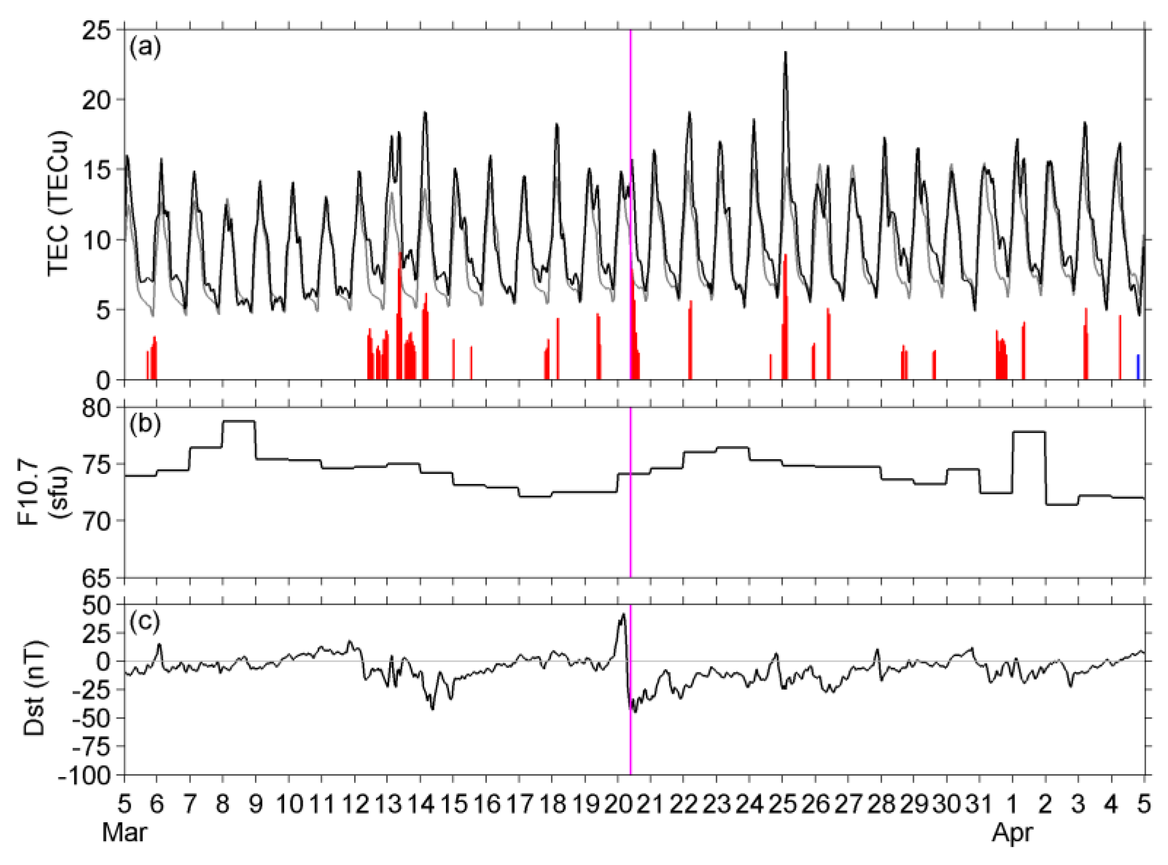
4.5. Observational Result on TEC Ionospheric Perturbations

Figure 16 illustrates the TEC analysis result for the first February EQ, together with the temporal variations of solar flux (F10.7) and the Dst index. The black curve in Figure 16 is the TEC value retrieved from CODE GIM, and the reference in the grey curve is the mean during the past 30 days. The red and blue bars in the figure display positive and negative anomalies, respectively; only the anomalies with a magnitude greater than 2 sigma are plotted here. All the major positive anomalies seem to be related to enhancements of solar and/or geomagnetic activities. Negative anomalies are weak, or persist for short periods, and only a noticeable one occurred on 4 February, but that one seems to be a conjugate of the negative anomaly in the southern hemisphere that propagated along the magnetic field line. Moreover, all of those positive and negative anomalies are global but not local ones. Hence, we think that there is no clear precursory anomaly of TEC in the upper ionosphere for this EQ.

Next, we move on to the TEC anomalies for the second March EQ. Similar to the first EQ, the TEC variation is presented in Figure 17 for the second equation. The TEC value over the EQ epicenter was again significantly affected by geomagnetic activities and showed positive anomalies before the second EQ. A considerable one among those anomalies was on 13 March (a week before the EQ). The accumulated hours of positive anomalies (i.e., how many hours the TEC is anomalous) peak around Japan, as in Figure 16 on 13 March. However, this TEC anomaly is probably not so convincing to be a pre-EQ effect, because the time series of the TEC value and Dst index show a high negative correlation in the daytime of 13 March.

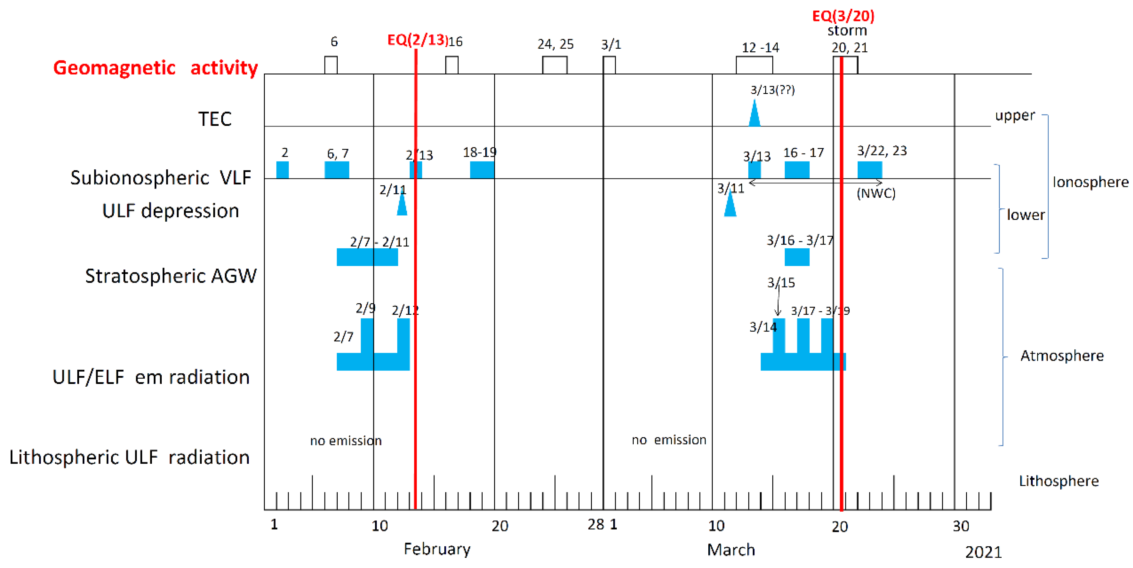
5. Summary and Discussion

In order to investigate the influence of lithospheric seismic activity on the upper regions, such as the atmosphere, stratosphere, and finally ionosphere (lowest part and upper F region), we summarize the observational facts revealed in each region but starting from the bottom source (or lithosphere). Figure 18 is the summary of observational results, paying the greatest attention to the temporal evolutions of different kinds of seismogenic phenomena, starting from the lowest region of the lithosphere up to the upper regions (atmosphere, stratosphere, lower ionosphere, and upper ionosphere of the F region). Since there were no significant precursors in January, we plotted different precursors only in February and March in Figure 18.

5.1. Lithospheric Effects

Lithospheric ULF radiation is a signature of lithospheric pre-EQ seismic activities or the generation of electric currents in the lithosphere [90,91,92]. As seen from Figure 2, there is just one possibility that ULF radiation might be observed at Kakioka only on 13 March during the whole period of January to March as an enhancement in the power spectra of Ph and Pz, about 1 week before the second March EQ. No ULF radiation signature was detected before the first EQ.

The detection of ULF radiation is known to be strongly dependent on the EQ magnitude and epicentral distance, and the possible detection range is about 100 km for M = 7 [72]. Therefore, the distances of the Kakioka observatory from those two EQs are 250–350 km, which might suggest that the geomagnetic observatory is located too far to find such ULF radiation. Nonetheless, we could detect ULF radiation for the 2011 Tohoku EQ [90], which was similar to the second EQ in this paper in the hypocenter condition, because the rupture area of the 2011 EQ was largely expanded down to the area close to the Kakioka station, enabling us to detect ULF radiation due to smaller distances between the ULF source and the station.

5.2. Atmospheric Effects

Atmospheric effects can be studied with the information of atmospheric ULF/ELF electromagnetic radiation. As seen from Figure 4 for the first EQ, the atmospheric ULF/ELF detected at NAK and SHI tends to appear from around 7 February until just after the EQ occurrence, but the most significant ULF/ELF emissions occur on 9 and 12 February. Further, the source regions of these ULF/ELF electromagnetic waves were estimated by the direction finding (Figure 6) to be close to the EQ epicenter, validating the seismogenic nature of those ULF/ELF waves.

On the other hand, as seen from Figure 5, similar ULF/ELF radiation was found to be detected at the same stations by enhancing the propagation parameter of delta S, confirming the nature of the seismogenic source. These electromagnetic emissions were again estimated to be located towards the direction of the EQ epicenter, as in Figure 7. These emissions were found to be observed continuously starting 14 March until the EQ occurrence, but the most conspicuous dates of these emissions were 15, 17, and 19 March.

Even though we try to pay our greatest attention to different hypocenter conditions of these EQs, we observed nearly the same ULF/ELF emissions. Additionally, those two EQs exhibited quite similar lead times, starting about 1 week before the EQ to the EQ day, being indicative of no effects of the local difference in hypothetical conditions on ULF/ELF emissions. For the 2011 Tohoku EQ, which is similar to the second EQ in this paper, Ohta et al. (2013) [70] succeeded in detecting clear ULF/ELF radiation a few days before the EQ, and the general morphologies of those emissions are very consistent with the present result.

Furthermore, Schekotov et al. (2017) [93] found the same ULF/ELF emissions before the recent Kumamoto EQs as well, and it seems that these ULF/ELF emissions are likely generated for any EQs, either inland-fault-type or oceanic-sea-type EQ. Recently, Fidani et al. (2020) [81] presented further evidence of these ULF/ELF emissions in the same frequency for the EQs in Europe with the use of their Italian network. Their characteristics, such as impulsive nature, frequency range, and lead time, are very consistent with our statistical summary by Schekotov and Hayakawa (2017) [82] and Hayakawa et al. (2019) [83], but unfortunately, they did not provide any statistical study as ours. The generation mechanism of these ULF/ELF emissions is extremely poorly understood, but Schekotov et al. (2020) [94] suggested a possibility of gas emanation from the trenches, leading to the modification of the atmosphere, such as the generation of electric fields or electric discharges. Actually, in the old days Blanchard (1963) [95] proposed the electrification of the atmosphere by bubbles with positive mist coming from the seabed, and Sorokin et al. (2020) [34] paid a lot of attention to the application of this idea to the explanation of different kinds of EQ precursors. Recently, Enomoto et al. (2020) [96] verified this hypothesis by examining the change in magnetic dip angle of the earth’s magnetic field, but unfortunately for an imminent precursor (just before, a few tens of minutes before the EQ) [38]. Probably this idea will be effectively applied to our short-term EQ precursor as well. The emanation of positively charged particles from the sea surface will form the electromagnetic force (EMF), which will result in the generation of electric fields in the atmosphere and ionosphere [34]. This may explain the ULF/ELF emissions as well. However, this idea cannot be applied to the first February EQ, and so the generation of ULF/ELF emissions for land EQs, including the case of our first EQ, the 2016 Kumamoto EQs, is open for discussion.

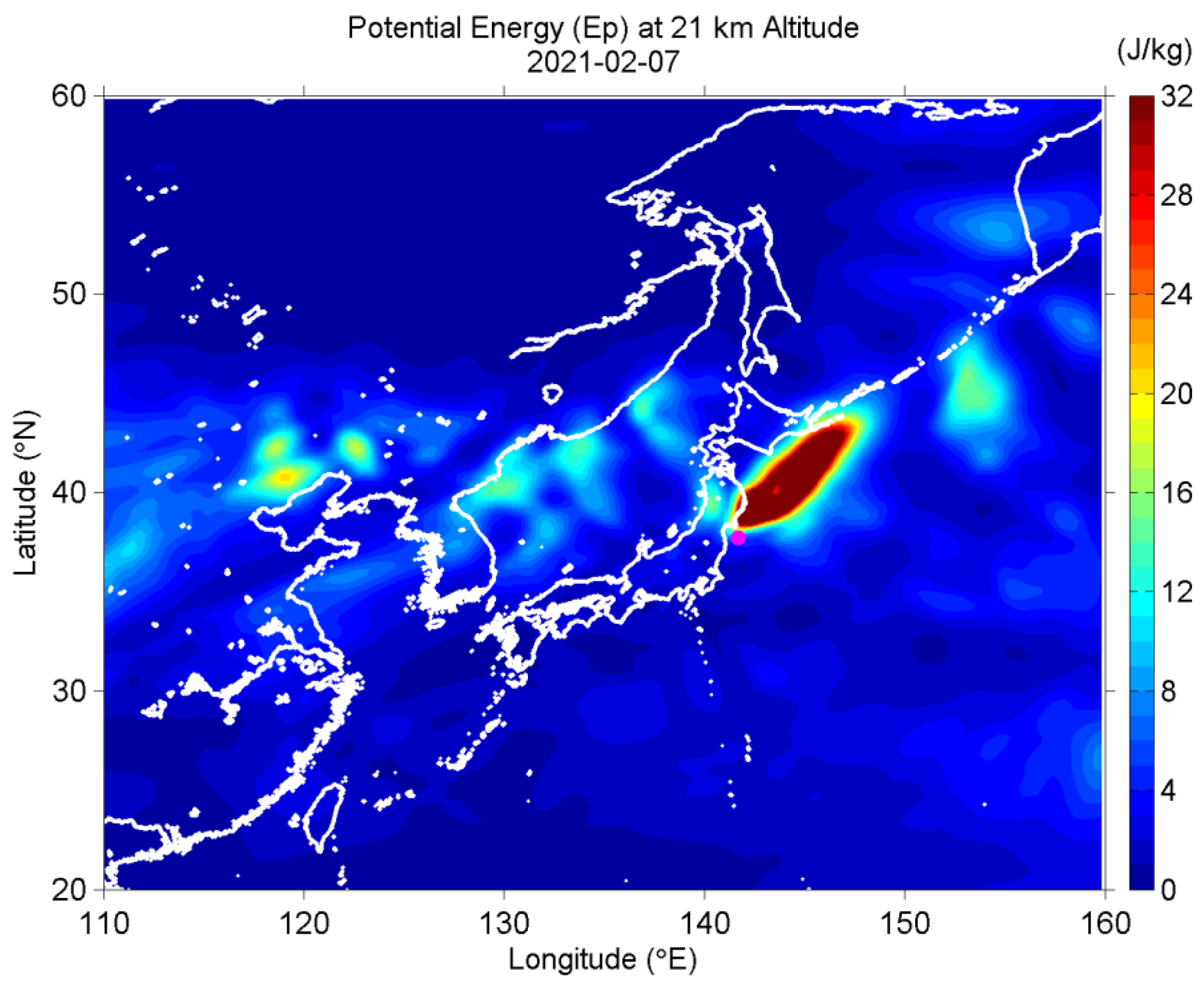
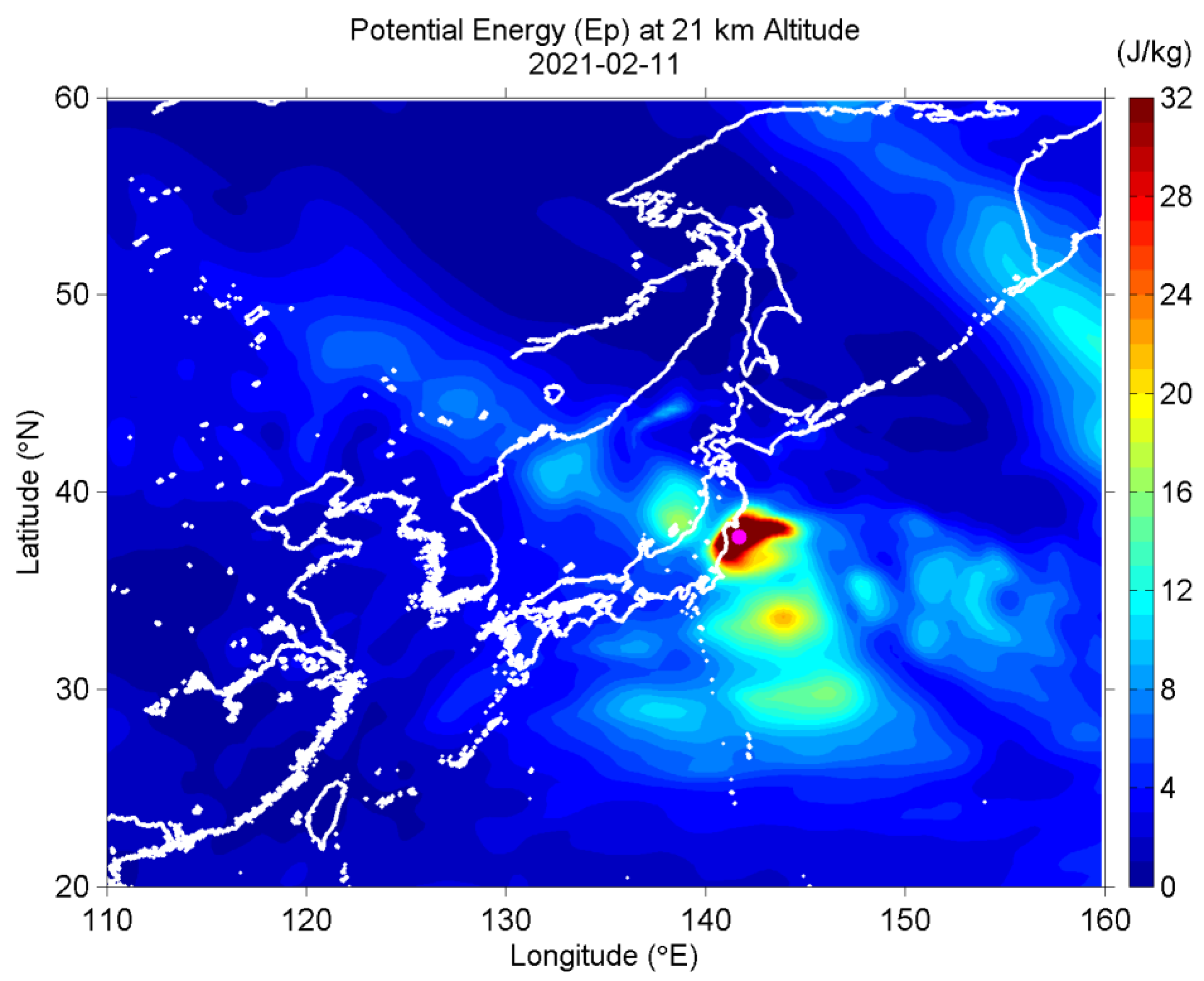
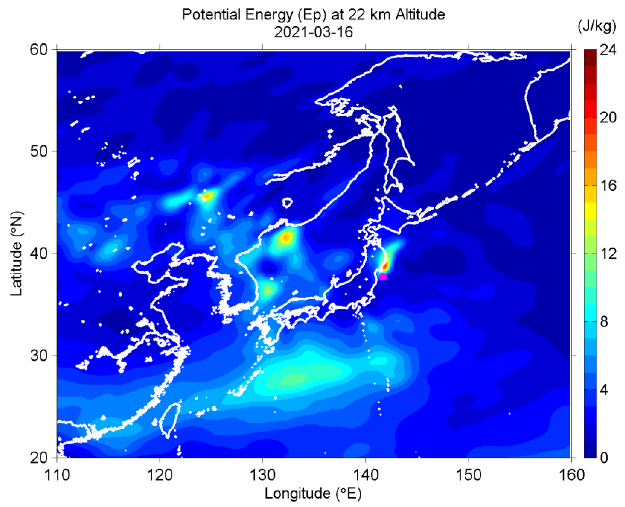
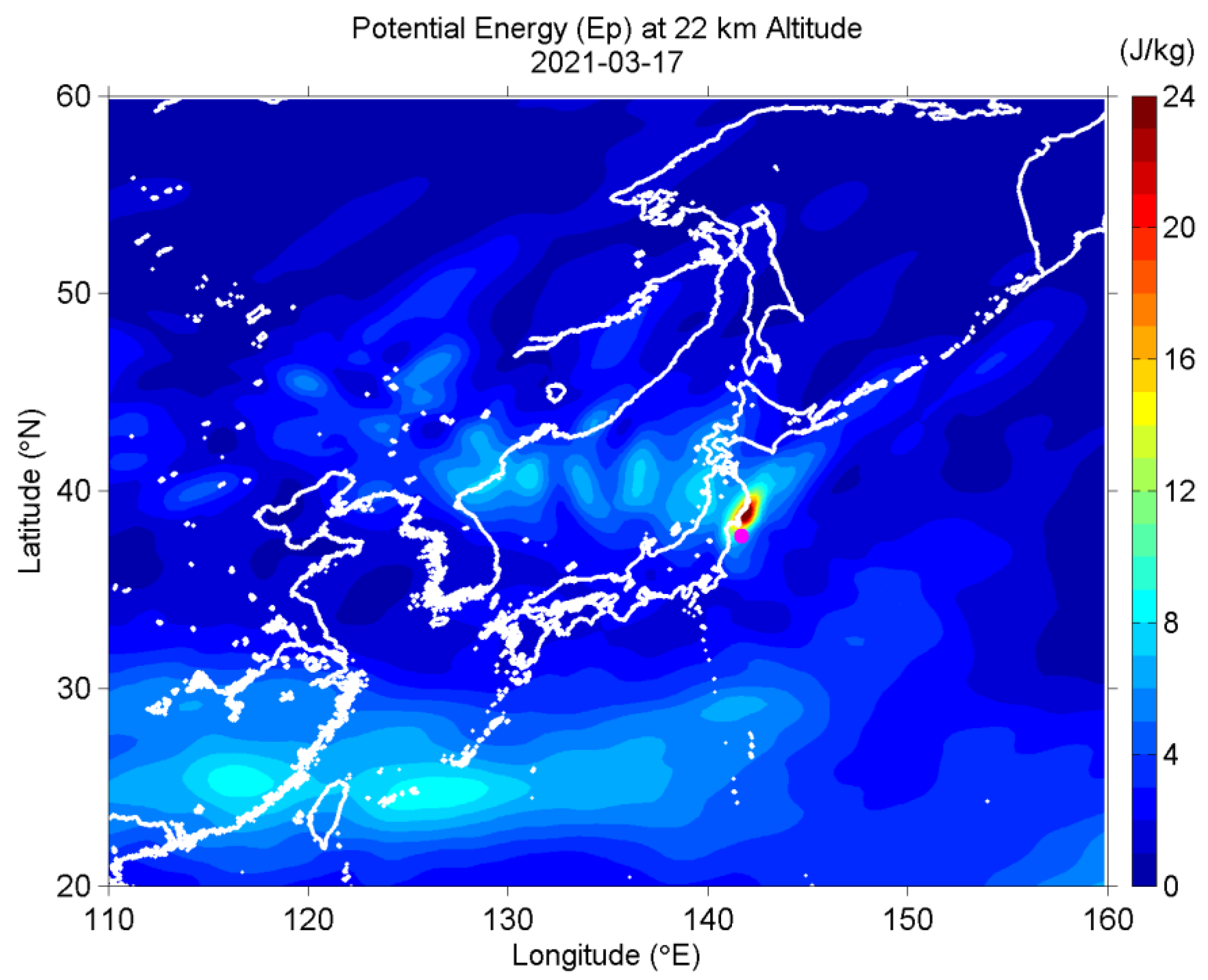
5.3. Stratospheric Effects

The study of stratospheric AGW, especially the potential energy Ep as given in Figure 8, Figure 9 and Figure 10, indicates that Ep exhibited a significant enhancement on 7–11 February, and many other AGW activities seem to be the consequence of winter weather systems. This AGW activity seemed to be detected over a large area from the EQ epicenter to the northeast direction on 7 February in the beginning, but finally, it was concentrated in a smaller mainland of Japan and in an expanded area with its center at the area right above the EQ epicenter on 11 February.

On the other hand, it seems for the second EQ (as seen from Figure 11, Figure 12 and Figure 13) that the seismogenic AGW perturbation was detected around the dates of 8 and 9 March, based on the combined consideration of weather maps over Japan. The spatial distribution of Ep at an altitude of 22 km on both days of 16 and 17 March indicates that the AGW activity is clearly distributed over the northeast of the EQ epicenter, but not right above the EQ epicenter, which is different from the case of the first EQ.

The second March EQ is very similar to the disastrous 2011 Tohoku EQ in the sense that for both EQs, rupture took place on the sea surface of the subducting plate (leading to tsunamis). Our latest work [54] indicated that AGW wave activity was generated seismogenically before the EQ, and that its spatial distribution extends northeastward and is only over the ocean side, being quite similar to that in the present paper. Furthermore, we found a very close correlation in temporal and spatial evolutions between the AGW activity and lower ionospheric perturbation as detected by VLF signals, giving a strong support to the AGW hypothesis of the LAIC process.

The difference for our two EQs is quite small in the excitation of AGW waves probably because the possible difference in the hypocenter condition does not play a significant role. Because the AGW waves for the first EQ are excited over the oceanic area, the enhancement of Ep even centered right above the EQ epicenter on 10 and 11 February. Nearly the same as the first EQ, AGWs are excited over the offshore or Pacific Ocean side of Japan for the second EQ, being consistent with the case of the 2011 Tohoku EQ [54,97] in which the temporal and spatial evolutions of AGW in the stratosphere and the lower ionospheric perturbation by subionospheric VLF/LF data are consistent with each other.

Of course, the most plausible source of the exciter of AGWs is the deformation or variation of the earth’s surface. In the old days, when we proposed the AGW hypothesis, we were always criticized that there is no evidence of surface deformation before an EQ. Recently, there have been several important published papers on the pre-EQ surface deformation based on the GPS, seismic measurements [55,98,99,100,101]. Chen et al. (2020) [99] found clear fluctuations in the frequency range in the earth’s surface deformation before large EQs, and suggested the presence of an AGW resonator in the lithosphere. Even if we accept their idea, how to relate this idea to the observational facts for our two EQs is open for discussion. An alternative source might be gas emanation from the ground, positive hole effect [62], and so forth.

5.4. Lower Ionospheric Perturbations

A lower ionospheric condition can be monitored with the use of a phenomenon of ULF depression. We try to give you a brief description of this effect. In the equatorial plane of the magnetosphere, different kinds of geomagnetic pulsations are generated due to the wave–particle interactions [9]. Especially irregular pulsations (Pis) are a popular one at nighttime; they propagate downwards along the magnetic line of forces and penetrate through the ionosphere and are received on the ground. Schekotov et al. (2006) [77] emphasized the importance of this phenomenon as a good indicator of short-term precursors to EQs.

As the mechanism of seismogenic ULF depression, the most probable mechanism is the enhanced absorption of magnetospheric pulsations when passing through the disturbed lower ionosphere [77,83] just as detected by subionospheric VLF/LF propagation data [16,21,25].

For both first and second EQs as seen from Figure 2, we observed a very clear phenomenon of ULF depression on 11 February before the first EQ and 11 March for the second EQ. The lead time of the first ULF depression was two days, and 9 days for the second EQ. As opposed to the case of lithospheric radiation, this phenomenon is generally considered to be very sensitive even for distant EQs.

Subionospheric VLF/LF data in Section 4.4 indicated that there are several detected propagation anomalies, but the one on 13 February (as an imminent precursor) is the only reliable one among several.

No information was obtained on the spatial distribution of the lower ionospheric perturbation only from the above Russian VLF/LF observation, but we can imagine based on our previous study [54] that the lower ionospheric perturbation might be elongated in the same direction as that of the AGW activity.

Additional evidence on the conductivity changes in the lower ionosphere and stratosphere was recently presented with the use of anomalous Schumann resonances for the same two EQs in this paper [102]. The anomalies of Schumann resonances near Nagoya were detected before and after each EQ (10–15 February for the first EQ and 19–24 March for the second EQ), which are characterized by enhancements in amplitudes of Schumann resonance harmonic frequencies.

5.5. Upper Ionospheric Effects

As seen from Figure 16 for the first EQ, all of the TEC anomalies (both negative and positive) seem to be related to the enhancements of solar and/or geomagnetic activities, so there seems to be no clear precursory anomaly of TEC for the first EQ.

The TEC variations for the second EQ, as seen from Figure 17, are seen to be well correlated with geomagnetic activities. Among those anomalies, a considerable one was on March 13. The accumulated hours of positive anomaly (i.e., how many hours the TEC was anomalous) were found to peak around Japan on 13 March, but this TEC anomaly was not so convincing, because the temporal variations of the TEC value and Dst seemed to indicate a high correlation in the daytime of this day, even though the geomagnetic disturbances in February and March were considered to be rather geomagnetically quiet since the maximum depression was only Dst = −50 nT (except for a 1 h spike at 00Z on 25 February).

6. Conclusions

Our initial intention of this paper was to try to find out any significant differences in the morphological characteristics of multiparameter precursors for two successive major EQs in February and March 2021 in order to have a further understanding of the LAIC process (i.e., which channel was working for each of the two EQs) because we paid attention to the significant difference in the seismological and geological conditions of the EQ hypocenters of those EQs. Figure 18 is a summary plot of various geophysical parameters as possible precursors studied in this paper as a function of day with respect to each EQ. The results in February and March are summarized because no significant anomalies were observed in January. We will list the important findings from the present study.

First of all, in sharp contrast with our initial anticipation that we might see a conspicuous difference of the occurrence of anomalies in various regions, including the lithosphere, atmosphere, and ionosphere, for the two February and March EQs with nearly the same magnitude (M~7), but with a significant difference in the seismological and geological conditions for the two EQs (e.g., an anomaly is present only for either one of the two EQs), we found in Figure 18 no such remarkable differences in the morphological occurrence of different precursors for the two EQs. This may indicate that such a local difference in hypocenter conditions for the two EQs does not play a significant role in the excitation of different precursors over a much wider area of EQ preparation.

Based on multiparameter observations, the most important finding is that all of the electromagnetic anomalies in different regions, such as atmospheric, stratospheric, and lower and upper ionospheric regions, are found to be concentrated only in a period from about 1 week before the EQ to the EQ day (or even after the EQ day). Actually, there are presently completely no anomalies in January and during the period between the two EQs. Hence, these observed anomalies are likely to be closely associated with each of the two EQs, probably as pre-EQ activity.

The most serious point when discussing the precursor studies is to pay the greatest attention to the reliability of each anomaly. Especially the effects of geomagnetic disturbances and meteorological perturbations can easily contaminate the detection of seismogenic anomalies, even though the general geomagnetic condition during our relevant period is rather geomagnetically quiet with the maximum Dst = −50 nT. However, recently some authors [103,104] have proposed an innovative hypothesis that ULF radiation thought to be an EQ precursor is triggered by solar activity just like geomagnetic storms, in which two phenomena of EQ ULF radiation and geomagnetic storms are regarded as brothers. This will be our future work to check. During the period of our interest, there exist clear and definite precursors to the EQs. Based on our previous extensive and statistical studies [8,82,83], we think that the most convincing precursor is atmospheric ULF/ELF emissions, which are identified to start about 1 week before each EQ to the EQ day. This is considered to be a very regular precursor as a promising candidate of short-term EQ prediction (see [83]), and is currently utilized in Kamchatka as a prospective EQ forecast [95]. The next reliable precursors are ionospheric perturbations as detected by ULF depression [83] on 11 February (2 days before the first EQ) and on 11 March (about 9 days before the second EQ), which means that the lower ionosphere must be perturbed around these dates. The last convincing precursor is the VLF/LF perturbation (lower ionospheric perturbation) [6,16,17,18,21,22,23,24,25,30] on the day of the first EQ as an imminent precursor.

Figure 18 may suggest that one particular anomaly of atmospheric ULF/ELF radiation seems to behave rather differently than other anomalies for the two EQs (especially the first February EQ) (i.e., being independent of other anomalies). Even though there may exist some uncertainty of the reliability of other anomalies in Figure 18, we can notice a likely chain (or cause-and-effect relationship) of the phenomena of the LAIC process for the February EQ in such a way that the effect in the lower altitude, such as AGWs, seems to propagate progressively upwards to the lower ionosphere. That is, it may be present that the lithospheric effect is propagating upwards to upper regions with some delays. On the other hand, all of the anomalies observed for the second March EQ are found to occur nearly simultaneously with each other, or in other words, different anomalies take place synchronously in time for the second March EQ. This difference in the temporal appearance of anomalies may give us some hint on the elucidation of the LAIC process with taking into account the expected temporal changes for possible LAIC hypotheses [29,34,35,51,52]. Of course, the way of excitation of AGW is still unclear, even though there are a few possible ways of AGW modulation, such as the direct deformation of the earth’s surface, the presence of an AGW resonator in the lithosphere [98,99], or local disturbances in the lithospheric conductivity by the modulation due to the emanation of charged gases in the EQ preparation phase [31,92,95]. Finally, we cannot say any definite conclusion on the LAIC mechanism.

As mentioned just above, the behavior of atmospheric ULF/ELF emission as the clearest precursor seems to be independent of other anomalies following the LAIC process, even though they are definitely the consequence of lithospheric or surface seismic activity. It seems that this phenomenon is not influencing the upper region (ionosphere), and that it is generated by the lithospheric effects including gas emanation and the associated discharges. In the future, we highly need data on the surface deformation (including GPS data, etc.) as performed by [98,99,100] as the initial agent of the LAIC process for the two EQs, especially because no lithospheric pre-EQ effect, such as lithospheric ULF radiation, was not clearly detected for the two EQs. This work is a relative multiparameter observation, but we require a much more elaborated multiparameter observation in the future.

References

1. Hayakawa, M. Earthquake Prediction with Radio Techniques; John Wiley and Sons: Singapore, 2015; 294p. [Google Scholar]
2. Kopytenko, Y.A.; Matiashvily, T.G.; Voronov, P.M.; Kopytenko, E.A.; Molchanov, O.A. Detection of ULF emissions connected with the Spitak earthquake and its aftershock activity based on geomagnetic pulsations data at Dusheti and Vardziya observatories. Phys. Earth Planet. Inter. 1990, 77, 85–95. [Google Scholar] [CrossRef]
3. Molchanov, O.A.; Kopytenko, Y.A.; Voronov, P.M.; Kopytenko, E.A.; Matiashvily, T.G.; Fraser-Smith, A.C.; Bernardi, A. Results of ULF magnetic field measurements near the epicenters of the Spitac (Ms = 6.9) and Loma Prieta (Ms = 7.1) earthquakes: Comparative analysis. Geophys. Res. Lett. 1992, 19, 1495–1498. [Google Scholar] [CrossRef]
4. Fraser-Smith, A.C.; Bernardi, A.; McGill, P.R.; Ladd, M.E.; Helliwell, R.A.; Villard, O.G., Jr. Low-frequency magnetic field measurements near the epicenter of the Ms 7.1 Loma Prieta earthquake. J. Geophys. Res. 1990, 17, 1465–1468. [Google Scholar]
5. Hayakawa, M.; Kawate, R.; Molchanov, O.A.; Yumoto, K. Results of ultra-low-frequency magnetic field measurements during the Guam earthquake of 8 August 1993. Geophys. Res. Lett. 1996, 23, 241–244. [Google Scholar] [CrossRef]
6. Hayakawa, M.; Molchanov, O.A.; Ondoh, T.; Kawai, E. The precursory signature effect of the Kobe earthquake on VLF subionospheric signals. J. Comm. Res. Lab. 1996, 43, 169–180. [Google Scholar]
7. Pulinets, S.A.; Boyarchuk, K. Ionospheric Precursors of Earthquakes; Springer: Berlin/Heidelberg, Germany, 2004; 315p. [Google Scholar]
8. Molchanov, O.A.; Hayakawa, M. Seismo Electromagnetics and Related Phenomena: History and Latest Results; TERRAPUB: Tokyo, Japan, 2008; 189p. [Google Scholar]
9. Surkov, V.; Hayakawa, M. Ultra and Extremely Low Frequency Electromagnetic Fields; Springer: Tokyo, Japan, 2014; 486p. [Google Scholar]
10. Sorokin, V.V.; Chmyrev, V.; Hayakawa, M. Electrodynamic Coupling of Lithosphere-Atmosphere-Ionosphere of the Earth; NOVA Science Pub. Inc.: New York, NY, USA, 2015; 355p. [Google Scholar]
11. Ouzounov, D.; Pulinets, S.; Hattori, K.; Taylor, P. (Eds.) Pre-Earthquake Processes: A Multidisciplinary Approach to Earthquake Prediction Studies; AGU Geophysical Monograph 234; Wiley: New York, NY, USA, 2018; 365p. [Google Scholar]
12. Varotsos, P.A. The Physics of Seismic Electric Signals; Terrapub: Tokyo, Japan, 2015; 388p. [Google Scholar]
13. Han, P.; Hattori, K.; Hirokawa, M.; Zhuang, J.; Chen, C.H.; Febriani, F.; Yamaguchi, H.; Yoshino, C.; Liu, J.Y.; Yoshida, S. Statistical analysis of ULF seismomagnetic phenomena at Kakioka, Japan, during 2001–2010. J. Geophys. Res. Space Phys. 2014, 119, 4998–5011. [Google Scholar] [CrossRef]
14. Ouzounov, D.; Pulinets, S.; Kafatos, M.C.; Taylor, P. Thermal radiation anomalies associated with major earthquakes. In Pre-Earthquakes Processes: A Multidisciplinary Approach to Earthquake Prediction Studies; AGU, Monograph; Ouzounov, D., Pulinets, S., Kafatos, M.C., Taylor, P., Eds.; Wiley: New York, NY, USA, 2018; pp. 259–277. [Google Scholar]
15. Genzano, N.; Filizzaola, C.; Hattori, K.; Pergola, N.; Tramutoli, V. Statistical correlation analysis between thermal infrared anomalies observed from MTSATs and large earthquakes occurred in Japan (2005–2015). J. Geophys. Res. Solid Earth 2021, 126, e2020JB020108. [Google Scholar] [CrossRef]
16. Hayakawa, M.; Kasahara, Y.; Nakamura, T.; Muto, F.; Horie, T.; Maekawa, S.; Hobara, Y.; Rozhnoi, A.A.; Solovieva, M.; Molchanov, O.A. A statistical study on the correlation between lower ionospheric perturbations as seen by subionospheric VLF/LF propagation and earthquakes. J. Geophys. Res. 2010, 115, A09305. [Google Scholar] [CrossRef]
17. Molchanov, O.A.; Hayakawa, M. Subionospheric VLF signal perturbations possibly related to earthquakes. J. Geophys. Res. 1998, 103, 17489–17504. [Google Scholar] [CrossRef]
18. Biagi, P.F.; Ermini, A. Geochemical and VLF-LF radio precursors of strong earthquakes. In Earthquake Prediction Studies: Seismo Electromagnetics; Hayakawa, M., Ed.; TERRAPUB: Tokyo, Japan, 2013; pp. 153–168. [Google Scholar]
19. Liu, J.Y.; Chen, Y.I.; Chuo, Y.J.; Chen, C.S. A statistical investigation of pre-earthquake ionospheric anomaly. J. Geophys. Res. 2006, 111, A05304. [Google Scholar] [CrossRef]
20. Le, H.; Liu, J.Y.; Liu, L. A statistical analysis of ionospheric anomalies before 736 M6.0+ earthquakes during 2002–2010. J. Geophys. Res. Atmos. 2011, 116, A02303. [Google Scholar] [CrossRef]
21. Rozhnoi, A.; Solovieva, M.; Molchanov, O.A.; Hayakawa, M. Middle latitude LF (40 kHz) phase variations associated with earthquakes for quiet and disturbed geomagnetic conditions. Phys. Chem. Earth 2004, 29, 589–598. [Google Scholar] [CrossRef]
22. Rozhnoi, A.; Solovieva, M.; Hayakawa, M. VLF/LF signals method for searching for electromagnetic earthquake precursors. In Earthquake Prediction Studies: Seismo Electromagnetics; Hayakawa, M., Ed.; TERRAPUB: Tokyo, Japan, 2013; pp. 31–48. ISBN 978-4-88704-163-9. [Google Scholar]
23. Maekawa, S.; Horie, T.; Yamauchi, T.; Sawaya, T.; Ishikawa, M.; Hayakawa, M.; Sasaki, H. A statistical study on the effect of earthquakes on the ionosphere, as based on the subionospheric LF of propagation data in Japan. Ann. Geophys. 2006, 24, 2219–2225. [Google Scholar] [CrossRef]
24. Chakhrabarti, S.K. (Ed.) Propagation Effects of Very Low Frequency Radio Waves; American Institute of Physics Conference Series; American Institute of Physics: College Park, MD, USA, 2010; Volume 1286. [Google Scholar]
25. Ray, S.; Chakrabarti, S.K.; Mondal, S.M.; Sasmal, S. Ionospheric anomaly due to seismic activities III: Correlation between nighttime VLF amplitude fluctuations and effective magnitudes in Indian sub-continent. Nat. Hazards Earth Syst. Sci. 2011, 11, 2699–2704. [Google Scholar] [CrossRef] [Green Version]
26. Liu, J.Y.; Chen, C.H.; Tsai, H.F. A statistical study on seismo-ionospheric precursors of the total electron content associated with 146 M 6.0 earthquakes. In Earthquake Prediction Studies: Seismo Electromagnetics; Hayakawa, M., Ed.; TERRAPUB: Tokyo, Japan, 2013; pp. 1–13. [Google Scholar]
27. Kon, S.; Nishihashi, M.; Hattori, K. Ionospheric anomalies possibly associated with M 6 earthquakes in Japan during 1998–2011: Case studies and statistical study. J. Asian Earth Sci. 2011, 41, 410–420. [Google Scholar] [CrossRef]
28. Parrot, M.; Li, M. Statistical analysis of the ionospheric density recorded by the satellite during seismic activity. In Pre-Earthquake Processes: A Multidisciplinary Approach to Earthquake Prediction Studies; AGU Monograph; Ouzounov, D., Pulinets, S., Kafatos, M.C., Taylor, P., Eds.; Wiley: New York, NY, USA, 2018; pp. 319–328. [Google Scholar]
29. Pulinets, S.; Ouzounov, D. Lithosphere-atmosphere-ionosphere coupling (LAIC) model—A unified concept for earthquake precursors validation. J. Asian Earth Sci. 2011, 41, 371–382. [Google Scholar] [CrossRef]
30. Hayakawa, M.; Asano, T.; Rozhnoi, A.; Solovieva, M. Very-low and low-frequency sounding of ionospheric perturbations and possible association with earthquakes. In Pre-Earthquake Processes: A Multidisciplinary Approach to Earthquake Prediction Studies; AGU, Monograph; Ouzounov, D., Pulinets, S., Kafatos, M.C., Taylor, P., Eds.; Wiley: New York, NY, USA, 2018; pp. 277–304. [Google Scholar]
31. Molchanov, O.; Fedorov, E.; Schekotov, A.; Gordeev, E.; Chebrov, V.; Surkov, V.; Rozhnoi, A.; Andreevsky, S.; Iudin, D.; Yunga, S.; et al. Lithosphere-atmosphere-ionosphere coupling as governing mechanism for preseismic short-term events in atmosphere and ionosphere. Nat. Hazards Earth Syst. Sci. 2004, 4, 757–767. [Google Scholar] [CrossRef] [Green Version]
32. Hayakawa, M.; Molchanov, O.A. NASDA/UEC team Summary report of NASADA Frontier Project. Phys. Chem. Earth 2004, 29, 617–625. [Google Scholar] [CrossRef]
33. De Santis, A.; Abbattista, C.; Alfonsi, L.; Amoruso, L.; Campuzano, S.A.; Carbone, M.; Cesaroni, C.; Cianchini, G.; Di Giovambattista, R.; Marchetti, D.; et al. Geosystems view of earthquakes. Entropy 2019, 21, 412. [Google Scholar] [CrossRef] [Green Version]
34. Sorokin, V.M.; Chmyrev, V.M.; Hayakawa, M. A review on electrodynamic influence of atmospheric processes to the ionosphere. Open J. Earthq. Res. 2020, 9, 113–141. [Google Scholar] [CrossRef] [Green Version]
35. Freund, F.T. Earthquake forewarning—A multidisciplinary challenge from the ground up to space. Acta Geophys. 2013, 61, 775–807. [Google Scholar] [CrossRef]
36. Akhoondzadeh, M.; De Santis, A.; Marchetti, D.; Piscini, A.; Cianchini, G. Multi precursors associated with the powerful Ecuador (Mw = 7.8) earthquake of 16 April 2016 using Swarm satellites data in conjunction with other multi-platform satellite and ground data. Adv. Space Res. 2018, 61, 248–263. [Google Scholar] [CrossRef] [Green Version]
37. Sasmal, S.; Chowdhury, S.; Kundu, S.; Politis, D.Z.; Potirakis, S.M.; Balasis, G.; Hayakawa, M.; Chakrabarti, S.K. Pre-seismic irregularities during the 2020 Samos (Greece) earthquake (M = 6.9) as investigated from multi-parameter approach by ground and space-based techniques. Atmosphere 2021, 12, 1059. [Google Scholar] [CrossRef]
38. Heki, K. Ionospheric electron enhancement preceding the 2011 Tohoku-oki earthquake. Geophys. Res. Lett. 2011, 38, L17312. [Google Scholar] [CrossRef] [Green Version]
39. Hayakawa, M.; Ito, T.; Smirnova, N. Fractal analysis of the ULF geomagnetic data associated with Guam earthquake on August 8, 1993. Geophys. Res. Lett. 1999, 26, 2797–2800. [Google Scholar] [CrossRef]
40. Ida, Y.; Hayakawa, M. Fractal analysis for the ULF data during the 1993 Guam earthquake to study prefracture criticality. Nonlinear Prcoesses Geophys. 2004, 13, 409–412. [Google Scholar] [CrossRef] [Green Version]
41. Eftaxias, K.; Potirakis, S.M.; Contoyiannis, Y. Four-stage model of earthquake generation in terms of fracture-induced electromagnetic emission: A review. In Complexity of Seismic Time Series; Chelidze, T., Vallianatos, F., Telesca, L., Eds.; Elsevier: Amsterdam, The Netherlands, 2018; pp. 437–502. [Google Scholar]
42. Varotsos, P.; Sarlis, N.; Skordas, E.S. Phenomena preceding major earthquakes interconnected through physical model. Ann. Geophys. 2019, 37, 315–324. [Google Scholar] [CrossRef] [Green Version]
43. Potirakis, S.M.; Contoyiannis, Y.; Koulouras, G.; Nomicos, C. Recent field observations indicating an earth system in critical condition before the occurrence of a significant earthquake. IEEE Geosci. Remote Sens. Lett. 2015, 12, 631–635. [Google Scholar] [CrossRef]
44. Potirakis, S.M.; Schekotov, A.; Asano, T.; Hayakawa, M. Natural time analysis on the ultra-low frequency magnetic field variations prior to the 2016 Kumamoto (Japan) earthquakes. J. Asian Earth Sci. 2018, 154, 419–427. [Google Scholar] [CrossRef]
45. Potirakis, S.M.; Contoyiannis, Y.; Schekotov, A.; Eftaxias, K.; Hayakawa, M. Evidence of critical dynamics in various electromagnetic precursors. Eur. Phys. J. Spec. Top. 2021, 230, 151–177. [Google Scholar] [CrossRef]
46. Liperovsky, V.A.; Meister, C.V.; Liperovskaya, E.V.; Bogdanov, V.V. On the generation of electric field and infrared radiation in aerosol clouds due to radon emanation in the atmosphere before earthquakes. Nat. Hazards Earth Syst. Sci. 2008, 8, 1199–1205. [Google Scholar] [CrossRef]
47. Sorokin, V.; Hayakawa, M. Plasma and electromagnetic effects caused by the seismic-related disturbances of electric current in the global circuit. Mod. Appl. Sci. 2014, 8, 61. [Google Scholar] [CrossRef] [Green Version]
48. Oyama, K.-I.; Devi, M.; Ryu, K.; Chen, C.H.; Liu, J.Y.; Liu, H.; Bankov, L.; Kodama, T. Modifications of the ionosphere prior to large earthquakes: Report from the Ionosphere Precursors Study Group. Geosci. Lett. 2016, 36. [Google Scholar] [CrossRef] [Green Version]
49. Sorokin, V.M.; Yaschenko, A.K.; Chmyrev, V.M.; Hayakawa, M. DC electric field formation in the mid-latitude ionosphere over typhoon and earthquake regions. Phys. Chem. Earth 2006, 31, 454–461. [Google Scholar] [CrossRef]
50. Hayakawa, M.; Kasahara, Y.; Nakamura, T.; Hobara, Y.; Rozhnoi, A.; Solovieva, M.; Molchanov, O.A.; Korepanov, K. Atmospheric gravity waves as a possible candidate for seismo-ionospheric perturbations. J. Atmos. Electr. 2011, 31, 129–140. [Google Scholar] [CrossRef] [Green Version]
51. Korepanov, V.; Hayakawa, M.; Yampolski, Y.; Lizunov, G. AGW as a seismo-ionospheric coupling responsible agent. Phys. Chem. Earth 2009, 34, 485–495. [Google Scholar] [CrossRef]
52. Lizunov, G.; Skorokhod, T.; Hayakawa, M.; Korepanov, V. Formation of ionospheric precursors of earthquakes—Probable mechanism and its substantiation. Open J. Earthq. Res. 2020, 9, 142. [Google Scholar] [CrossRef] [Green Version]
53. Yang, S.S.; Asano, T.; Hayakawa, M. Abnormal gravity wave activity in the stratosphere prior to the 2016 Kumamoto earthquakes. J. Geophys. Res. Space Phys. 2019, 124, 1410–1425. [Google Scholar] [CrossRef]
54. Yang, S.S.; Hayakawa, M. Gravity wave activity in the stratosphere before the 2011 Tohoku earthquake as the mechanism of lithosphere-atmosphere-ionosphere coupling. Entropy 2020, 22, 110. [Google Scholar] [CrossRef] [Green Version]
55. Yang, S.S.; Potirakis, S.M.; Sasmal, S.; Hayakawa, M. Natural time analysis of Global Navigation Satellite System surface deformation: The case of the 2016 Kumamoto earthquakes. Entropy 2020, 22, 674. [Google Scholar] [CrossRef]
56. Piersanti, M.; Marterassi, M.; Battiston, R.; Carbone, V.; Cicone, C.; D’Angelo, G.; Diego, P.; Ubertini, P. Magnetospheric-ionospheric-lithospheric coupling model. 1: Observations during the 5 August 2018 Bayan earthquake. Remote Sens. 2020, 12, 3299. [Google Scholar] [CrossRef]
57. Carbone, V.; Piersanti, M.; Materassi, M.; Battison, R.; Lipreti, F.; Ubertini, P. A mathematical model of lithosphere-atmosphere-ionosphere coupling for seismic events. Sci. Rep. 2021, 11, 868. [Google Scholar] [CrossRef]
58. Galper, A.M.; Dimitrenko, V.B.; Nikitina, N.V.; Grachev, V.M.; Ulin, S.E. Interrelation between high-energy charged particle fluxes in the radiation belt and seismicity of the Earth. Cosm. Res. 1989, 27, 789. [Google Scholar]
59. Galperin, Y.I.; Gladyshev, V.A.; Jordjio, N.V.; Larkina, V.I. Precipitation of high-energy captured particles in the magnetosphere above the epicenter of an incipient earthquake. Cosm. Res. 1992, 30, 89–106. [Google Scholar]
60. Sgrigna, V.; Carota, L.; Conti, M.; Galper, A.M.; Koldashov, S.V.; Murashov, A.M.; Picozza, P.; Scrimaglio, R.; Stangi, L. Correlations between earthquakes and anomalous particle bursts from SAMPEX/PET satellite observations. J. Atmos. Sol.-Terr. Phys. 2005, 67, 1448–1462. [Google Scholar] [CrossRef]
61. Fidani, C.; Battiston, R.; Burger, W.J. A study of the correlation between earthquakes and NOAA satellite energetic particle bursts. Remote Sens. 2010, 9, 2170–2182. [Google Scholar] [CrossRef] [Green Version]
62. Freund, F.; Ouillon, G.; Scoville, J.; Sornett, D. Earthquake precursors in the light of peroxy defects theory: Critical review of systematic observations. Eur. Phys. J. Spec. Top. 2021, 230, 7–46. [Google Scholar] [CrossRef]
63. Molchanov, O.A.; Hayakawa, M.; Miyaki, K. VLF/LF sounding of the lower ionosphere to study the role of atmospheric oscillations in the lithosphere-ionosphere coupling. Adv. Polar Up. Atmos. Res. 2001, 15, 146–158. [Google Scholar]
64. Miyaki, K.; Hayakawa, M.; Molchanov, O.A. The role of gravity waves in the lithosphere-ionosphere coupling as revealed from the subionospheric LF propagation data. In Seismo Electromagnetics: Lithosphere-Atmosphere-Ionosphere Coupling; Hayakawa, M., Molchanov, O.A., Eds.; TERRAPUB: Tokyo, Japan, 2002; pp. 229–232. [Google Scholar]
65. Shvets, A.V.; Hayakawa, M.; Molchanov, O.A.; Ando, Y. A study of ionospheric response to regional seismic activity by VLF radio sounding. Phys. Chem. Earth 2004, 29, 627–637. [Google Scholar] [CrossRef]
66. Sasmal, S.; Chakhrabarti, S.K.; Ray, S. Unusual behavior of Very Low Frequency signal during the earthquake at Honshu/Japan. Indian J. Phys. 2014, 88, 1013–1019. [Google Scholar] [CrossRef]
67. Rozhnoi, A.A.; Solovieva, M.; Molchanov, O.; Biagi, P.F.; Hayakawa, M. Observational evidence of atmospheric gravity waves induced by seismic activity from analysis of subionospheric LF signal spectra. Nat. Hazards Earth Syst. Sci. 2007, 7, 625–628. [Google Scholar] [CrossRef]
68. Dobrovolsky, I.R.; Zubrov, S.I.; Myachkin, V.I. Estimation of the size of earthquake preparation zone. Pure Appl. Geophys. 1979, 117, 1025–1044. [Google Scholar] [CrossRef]
69. Ruzhin, Y.Y.; Depueva, A.K. Seismoprecursors in space as plasma and wave anomalies. J. Atmos. Electr. 1996, 16, 271–288. [Google Scholar] [CrossRef]
70. Ohta, K.; Izutsu, J.; Schekotov, A.; Hayakawa, M. The ULF/ELF electromagnetic radiation before the 11 March 2011 Japanese earthquake. Radio Sci. 2013, 48, 589–596. [Google Scholar] [CrossRef]
71. Hattori, K. ULF geomagnetic changes associated with large earthquakes. Terr. Atmos. Ocean. Sci. 2004, 15, 329–360. [Google Scholar] [CrossRef] [Green Version]
72. Hayakawa, M.; Hattori, K.; Ohta, K. Monitoring of ULF (ultra-low-frequency) geomagnetic variations associated with earthquakes. Sensors 2007, 7, 1108–1122. [Google Scholar] [CrossRef] [Green Version]
73. Currie, J.L.; Waters, C.L. On the use of geomagnetic indices and ULF waves for earthquake precursor signatures. J. Geophys. Res. Space Phys. 2014, 119, 992–1003. [Google Scholar] [CrossRef]
74. Yusof, K.A.; Abdullay, M.; Hamid, N.S.A.; Ahadi, S.; Yoshikawa, A. Correlations between earthquake properties and characteristics of possible ULF geomagnetic precursors over multiple earthquakes. Universe 2021, 7, 20. [Google Scholar] [CrossRef]
75. Molchanov, O.A.; Schekotov, A.Y.; Fedorov, E.N.; Belyaev, G.G.; Gordeev, E.E. Preseismic ULF electromagnetic effect from observation at Kamchatka. Nat. Hazards Earth Syst. Sci. 2003, 3, 203–209. [Google Scholar] [CrossRef]
76. Molchanov, O.A.; Schekotov, A.Y.; Fedorov, E.; Belyaev, G.G.; Gordeev, E.E. Preseismic ULF electromagnetic effect and possible interpretation. Ann. Geophys. 2004, 47, 119–131. [Google Scholar]
77. Schekotov, A.; Molchanov, O.; Hattori, K.; Fedorov, E.; Gladyshev, V.A.; Belyaev, G.G.; Chebrov, V.; Sinitsin, V.; Gordeev, E.; Hayakawa, M. Seismo-ionospheric depression of the ULF geomagnetic fluctuations at Kamchatka and Japan. Phys. Chem. Earth 2006, 31, 313–318. [Google Scholar] [CrossRef]
78. Schekotov, A.Y.; Molchanov, O.A.; Hayakawa, M.; Fedorov, E.N.; Chebrov, V.N.; Sinitsin, V.I.; Gordeev, E.F.; Belyaev, G.G.; Yagova, N.V. ULF/ELF magnetic field variation from atmosphere by seismicity. Radio Sci. 2007, 42, RS6S90. [Google Scholar] [CrossRef]
79. Hayakawa, M.; Schekotov, A.; Fedorov, E.; Hobara, Y. On the ultra-low-frequency magnetic field depression for three huge oceanic earthquakes in Japan and in the Kurile islands. Earth Sci. Res. 2013, 2, 33. [Google Scholar] [CrossRef] [Green Version]
80. Schekotov, A.; Chebrov, D.; Hayakawa, M.; Belyaev, G. Estimation of the epicenter position of. Kamchatka earthquakes. Pure Appl. Geophys. 2021, 178, 813–821. [Google Scholar] [CrossRef]
81. Fidani, C.; Orsini, M.; Iezzi, G.; Vicentini, N.; Stoppa, F. Electric and magnetic recordings by Chieti CIEN station during the intense 2016–2017 seismic swarms in central Italy. Front. Earth Sci. 2020, 8, 451. [Google Scholar] [CrossRef]
82. Schekotov, A.; Fedorov, E.; Molchanov, O.A.; Hayakawa, M. Low frequency electromagnetic precursors as a prospect for earthquake prediction. In Earthquake Prediction Studies: Seismo Electromagnetics; Hayakawa, M., Ed.; TERRAP: Tokyo, Japan, 2013; pp. 81–99. [Google Scholar]
83. Hayakawa, M.; Schekotov, A.; Izutsu, J.; Nickolaenko, A.P. Seismogenic effects in ULF/ELF/VLF electromagnetic waves. Int. J. Electron. Appl. Res. 2019, 6, 1–86. [Google Scholar] [CrossRef]
84. Fowler, R.A.; Kotick, B.J.; Elliot, R.D. Polarization analysis of natural and artificially induced geomagnetic micropulsations. J. Geophys. Res. 1967, 72, 2871–2875. [Google Scholar] [CrossRef]
85. Herbach, H.; Bell, B.; Berrisford, P.; Hirahara, S.; Horanyi, A.; Munoz-Sabataer, J.; Nicolas, J.; Peubey, C.; Radu, R.; Schepers, D.; et al. The ERA5 global reanalysis. Q. J. R. Meteorol. Soc. 2020, 146, 1999–2049. [Google Scholar] [CrossRef]
86. Kikuchi, T.; Evans, D.S. Quantitative study of substorm-associated VLF phase anomalies and precipitating energetic electrons on November 13, 1979. J. Geophys. Res. Space Phys. 1983, 88, 871–880. [Google Scholar] [CrossRef]
87. Peter, W.B.; Chevalier, M.W.; Inan, U.S. Perturbations of midlatitude subionospheric VLF signals associated with lower ionospheric disturbances during major geomagnetic storms. J. Geophys. Res. Space Phys. 2006, 111, A3. [Google Scholar] [CrossRef]
88. Rozhnoi, A.; Molchanov, O.; Solovieva, M.; Gladyshev, V.; Akentieva, O.; Berthelier, J.J.; Parrot, M.; Lefeuvre, F.; Hayakawa, M.; Castellana, L.; et al. Possible seismo-ionosphere perturbations revealed by VLF signals collected on ground and on a satellite. Nat. Hazards Earth Syst. Sci. 2007, 7, 617–624. [Google Scholar] [CrossRef] [Green Version]
89. Schaer, S. Mapping and Predicting the Earth’s Ionosphere Using the Global Positioning System. Ph.D. Thesis, Astronomical Institute, University of Berne, Berne, Switzerland, 1999. [Google Scholar]
90. Hayakawa, M.; Schekotov, A.; Potirakis, S.M.; Eftaxias, K. Criticality features in ULF magnetic fields prior to the 2011 Tohoku earthquake. Proc. Jpn. Acad. Ser. B 2015, 91, 25–30. [Google Scholar] [CrossRef] [PubMed] [Green Version]
91. Molchanov, M.; Hayakawa, M. Generation of ULF electromagnetic emissions by microfracturing. Geophys. Res. Lett. 1995, 22, 3091–3094. [Google Scholar] [CrossRef]
92. Tzanis, A.; Vallianatos, F. A physical model of electric earthquake precursors due to crack propagation and the motion of charged edge dislocations. In Seismo Electromagnetics: Lithosphere-Atmosphere-Ionosphere Coupling; Hayakawa, M., Molchanov, O.A., Eds.; TERRAPUB: Tokyo, Japan, 2002; pp. 117–130. [Google Scholar]
93. Schekotov, A.; Izutsu, J.; Asano, T.; Potirakis, S.M.; Hayakawa, M. Electromagnetic precursors to the 2016 Kumamoto earthquakes. Open J. Earthq. Res. 2017, 6, 168–179. [Google Scholar] [CrossRef] [Green Version]
94. Schekotov, A.; Chebrov, D.; Hayakawa, M.; Belyaev, G.; Berseneva, N. Short-term earthquake prediction at Kamchatka using low-frequency magnetic field. Nat. Hazards 2020, 100, 735–755. [Google Scholar] [CrossRef]
95. Blanchard, D.C. The electrification of the atmosphere by particles from bubbles in the sea. Prog. Oceanogr. 1963, 1, 73–202. [Google Scholar] [CrossRef]
96. Enomoto, Y.; Heki, K.; Yamabe, Y.; Sugiura, S.; Kondo, H. A possible casual mechanism of geomagnetic variations as observed immediately before and after the 2011 Tohoku-oki earthquake. Open J. Earthq. Res. 2020, 9, 33. [Google Scholar] [CrossRef] [Green Version]
97. Hayakawa, M.; Rozhnoi, A.; Solovieva, M.; Hobara, Y.; Ohta, K.; Schekotov, A.; Fedorov, E. The lower ionospheric perturbation as a precursor to the 11 March 2011 Japan earthquake. Geomat. Nat. Hazards Risk 2013, 4, 275–287. [Google Scholar] [CrossRef] [Green Version]
98. Kamiyama, M.; Sugito, M.; Kuse, M.; Schekotov, A.; Hayakawa, M. On the precursors to the 2011 Tohoku earthquake: Crustal movements and electromagnetic signatures. Geomat. Nat. Hazards Risk 2014, 7, 471–492. [Google Scholar] [CrossRef] [Green Version]
99. Chen, C.H.; Lin, L.C.; Yeh, T.K.; Wen, S.; Yu, H.; Yu, C.; Gao, Y.; Han, P.; Sun, Y.Y.; Liu, J.Y.; et al. Determination of epicenters before earthquakes utilizing far seismic and GNSS data: Insights from ground vibrations. Remote Sens. 2020, 12, 3252. [Google Scholar] [CrossRef]
100. Chen, C.H.; Sun, Y.Y.; Wen, S.; Han, P.; Lin, L.C.; Yu, H.; Zhang, X.; Gao, Y.; Tang, C.C.; Lin, C.H.; et al. Spatiotemporal changes of seismicity rate during earthquakes. Nat. Hazards Earth Syst. Sci. 2020, 20, 3333–3341. [Google Scholar] [CrossRef]
101. Bedford, J.R.; Moreno, M.; Deng, Z.; Oncken, O.; Schurr, B.; John, T.; Baez, T.C.; Bevis, M. Months-long thousand-kilometre-scale wobbling before great subduction earthquakes. Nature 2020, 580, 628–639. [Google Scholar] [CrossRef]
102. Hayakawa, M.; Izutsu, J.; Schekotov, A.; Galuk, Y.P.; Nickolaenko, A.P.; Kudintseva, I.G. Anomalies of Schumann resonances as observed near Nagoya associated with the huge (M~7) Tohoku offshore earthquakes in 2021. J. Atmos. Sol.-Terr. Phys. 2021, 225, 105761. [Google Scholar] [CrossRef]
103. Marchitelli, V.; Harabaglia, P.; Troise, C.; De Natale, G. On the correlation between solar activity and large earthquakes worldwide. Sci. Rep. 2020, 10, 11495. [Google Scholar] [CrossRef] [PubMed]
104. Anagnostopoulos, G.; Spyroglou, I.; Rigas, L.A.; Preka-Papadama, P.; Mavromichalaki, H.; Kiosses, I. The sun as a significant agent provoking earthquakes. Eur. Phys. J. Spec. Top. 2021, 230, 287–333. [Google Scholar] [CrossRef]
Figure 1. Locations of the ULF fluxgate magnetometer (black square) at Kakioka (KAK), ULF/ELF induction magnetometers (black rhombs) at Nakatsugawa (NAK) and Shinojima (SHI) and epicenters of the two EQs (circles) with a magnitude of M > 7 in the period of January–March 2021. The wide gray dash lines indicate the position of the trenches, and the black thin dash–dot lines in the main land display the location of the main faults.
Geosciences 11 00481 g001
Figure 2. Locations of a VLF/LF observing station (PTK in Kamchatka) and VLF/LF transmitters of JJY and JJI (in Japan), together with the corresponding wave sensitive (Fresnel) zone for each propagation path, including an additional transmitter of NWC (Australia). Only the second EQ epicenter is also plotted.
Geosciences 11 00481 g002
Figure 3. The evolution of seismicity, geomagnetic activity, and ULF magnetic field characteristics in the interval of 3 months from 1 January to 31 March 2021. The first two are represented on the top panel by the local seismicity index K L S and the geomagnetic activity Kp index. The average values of the horizontal Fh, vertical Fz component, and their ratio Pz/h are presented in the next three panels. Evolutions of depression Deph and its variation δ D e p h i are depicted in the two bottom panels. The vertical red broken lines indicate the occurrence times of the two EQs.
Geosciences 11 00481 g003
Figure 4. The evolution of seismicity, geomagnetic activity, and parameter of ULF/ELF magnetic field radiation over the interval of 7–14 February 2021 for the first EQ. The top panel shows evolutions of seismicity K L S and geomagnetic activity Kp. The next panels display spectra and their daily maximum values observed in NAK (second and third panels) and SHI (fourth and fifth panels).
Geosciences 11 00481 g004
Figure 5. The evolution of seismicity, geomagnetic activity, and parameter of ULF/ELF magnetic field radiation over the interval of 14–20 March 2021 for the second EQ. The top panel shows evolutions of seismicity K L S and geomagnetic activity Kp. The next two panels display ∆S spectra and their daily maximum values observed in SHI.
Geosciences 11 00481 g005
Figure 6. Evolutions of the azimuth distributions of ULF/ELF radiation for the first EQ on 7–12 February 2021 observed in Nakatsugawa (NAK) and Shinojima (SHI) are shown on two rows of round panels. The three upper panels illustrate the positions of the modes (main lobes) of the azimuthal distributions. The positions of the magnetometers are depicted by two rhombuses and the EQ by a circle.
Geosciences 11 00481 g006
Figure 7. The evolution of the azimuthal distribution of ULF/ELF radiation for the second EQ on 14–20 March 2021 observed in SHI. The upper panel shows the position of the main lobe of the azimuthal distribution observed on 17 March.
Geosciences 11 00481 g007
Figure 8. Temporal evolution of altitude profile of potential energy Ep over the epicenter. The vertical magenta line indicates the occurrence time of the first EQ. The red and blue arrows at the bottom of the figure indicate the passing of several weather systems, and the brown rectangle indicates a possible precursor to the first EQ.
Geosciences 11 00481 g008
Figure 9. Spatial distribution of Ep at a specific altitude of 21 km on 7 February 2021. The magenta dot indicates the EQ epicenter of the first February EQ.
Geosciences 11 00481 g009
Figure 10. Same as in Figure 9, but on 11 February 2021.
Geosciences 11 00481 g010
Figure 11. Same as in Figure 8, but for the second EQ.
Geosciences 11 00481 g011
Figure 12. Same as in Figure 9, but for the second March EQ at a specific altitude of 22 km on 16 March. The color scaling is also different from that in Figure 9.
Geosciences 11 00481 g012
Figure 13. Same as in Figure 12, but for the second EQ at an altitude of 22 km on 17 March.
Geosciences 11 00481 g013
Figure 14. VLF/LF propagation anomaly for the first February EQ. The first plot depicts the temporal variation (as a function of day) of atmospheric pressure at Kamchatka in hPa. The second and third panels refer to the daily variations of signal amplitude (in relative unit) for the two propagation paths of JJI-PTK and JJY-PTK. The horizontal dotted lines indicate −2 sigma lines (sigma is standard deviation), and amplitudes below this threshold are regarded as VLF/LF anomalies.
Geosciences 11 00481 g014
Figure 15. Same as in Figure 14, but for the second March EQ. Three daily variations of signal amplitudes for the three propagation paths of JJI-PTK (first panel), JJI-PTK (second panel), and NWC-PTK (bottom panel). The ordinate is signal amplitude in relative unit (red), and the horizontal lines are all −2 sigma level for each propagation path.
Geosciences 11 00481 g015
Figure 16. Temporal variation of TEC value for the first February EQ (a). The grey lines indicate the mean during the past 30 days. The red and blue bars indicate positive and negative anomalies, respectively; and only anomalies greater than 2 sigma are plotted. Additionally, solar flux (F10.7) (b) and the Dst index (c) are plotted.
Geosciences 11 00481 g016
Figure 17. Same as in Figure 16, but for the second EQ.
Geosciences 11 00481 g017
Figure 18. Summary of different possible precursors in the lithosphere, atmosphere, and lower and upper ionosphere as indications of LAIC effects. The anomalies in February and March are summarized because there are no anomalies in January.
Geosciences 11 00481 g018
Publisher’s Note: MDPI stays neutral with regard to jurisdictional claims in published maps and institutional affiliations.