Spring Water Geochemistry: A Geothermal Exploration Tool in the Rhenohercynian Fold-and-Thrust Belt in Belgium

Abstract

Spring water geochemistry is applied here to evaluate the geothermal potential in Rhenohercynian fold and thrust belt around the deepest borehole in Belgium (Havelange borehole: 5648 m MD). Fifty springs and (few) wells around Havelange borehole were chosen according to a multicriteria approach including the hydrothermal source of “Chaudfontaine” (T ≈ 36 °C) taken as a reference for the area. The waters sampled, except Chaudfontaine present an in-situ T range of 3.66–14.04 °C (mean 9.83 °C) and a TDS (dry residue) salinity range of 46–498 mg/L. The processing methods applied to the results are: hierarchical clustering, Piper and Stiff diagrams, TIS, heat map, boxplots, and geothermometry. Seven clusters are found and allow us to define three main water types. The first type, locally called “pouhon”, is rich in Fe and Mn. The second type contains an interesting concentration of the geothermal indicators: Li, Sr, Rb. Chaudfontaine and Moressée (≈5 km East from the borehole) belong to this group. This last locality is identified as a geothermal target for further investigations. The third group represents superficial waters with frequently high NO₃ concentration. The application of conventional geothermometers in this context indicates very different reservoir temperatures. The field of applications of these geothermometers need to be review in these geological conditions.

1. Introduction

Geothermal exploration, as any subsurface resource evaluation, requires a multidisciplinary approach (e.g., geological mapping, geophysics, geochemistry) and usually follows a downscaling approach starting from a regional scale toward a shortlist of potential sites for more detailed investigations [1,2]. These sites usually show surface indicators of the presence of a geothermal resource at depth. The nature of these indicators varies in the shape of hydrothermal springs, vapor exhalation, or sinter deposition. These indicators can even take the shape of biological manifestations as bacterial mats (e.g., [3,4,5], presence of bacterial community on travertine deposits [6] or even saline water tolerant plant and animal concentrations (e.g., eels) [7]). Even if such indicators are interesting clues in evaluating the geothermal fields, not all of them show obvious indicators at ground surface of their presence. An example of such blind geothermal fields is the Great Basin region in Nevada, which was recognized as a high-enthalpy important geothermal field without surface indicators [2,8]. Other blind geothermal systems were explored and/or developed in New Zealand, Hawaii, Indonesia [9,10]. Some of these blind geothermal systems were even discovered while targeting other resources (oil and gas, coal, minerals) for example in southern California [11], in Nevada [12], or in Belgium [13,14]. A common denominator of these blind geothermal systems is the presence of a cap formation, which hides many indicators of the presence of the geothermal resource.

The specificities and challenges to evaluate the geothermal potential of deep meta-sedimentary formations such as those encountered by the Havelange borehole (Belgium) are numerous: the Havelange borehole was drilled for gas exploration, hence, some important tasks/parameters for geothermal exploration were not conducted or recorded. The borehole site location is, therefore, fixed and not necessarily located in the most promising location for the development of a geothermal system in the region. The aforementioned downscaling approach frequently used in geothermal exploration cannot be applied. Another issue is the lack of information regarding the deep fluid flows and fluid composition since formation water inflows were thwarted by drilling mud injections as usual in drilling operation. It is important to note that two thick aquifer formations were encountered in this borehole [15]: (i) limestones and dolomites of Frasnian-Givetian ages (MD: 606–1595 m) and calcareous-sandstones of Eifelian (MD: 1610–1700 m); (ii) the fractured continuous quartzites of the Upper Praguian (MD: 4365–4554 m and 4639–4778 m). These two aquifers are separated from each other by more than 2000 m of aquiclude shales and slates of Emsian and Upper Praguian ages (from MD 1920 m to 4300 m). The aquifer character of the carbonate formations of Frasnian and Givetian is attested by significant mud losses during drilling and by few artesian events while adding drill rods. With regard to the aquifer and fractured Pragian quartzites, there are indirect indications that support this hypothesis: significant losses of drilling mud, sudden increases of mud temperature, poor Dipmeter log not showing consistent dips, Sonic log showing low speed peaks (fractures). The quarzitic Praguian, host rock for the geothermal reservoir, must be regarded as tight but permeable fracture zones that could represent potential geothermal targets. The logging data (gamma-ray, sonic, dipmeter) acquired during the 1980s provide only partial information regarding fracture networks, especially in comparison with modern logging data.

The punctual bottom hole temperature measurements indicate a mean moderate geothermal gradient of 22 °C/km but a sudden increase to 30 °C/km from 4400 m to the deepest parts of the borehole to reach a corrected value of 126 °C at 5369 m (MD-5277 VD) [15,16]. If the geothermal resource exists, it corresponds to a blind geothermal system with no obvious surface indicator of the resource.

Besides all these challenges, the existence of a deep borehole cross cutting a full (meta-)sedimentary sequence is not so common. All the cores, the cuttings, and most of the documents (e.g., logs) are still available and conserved by the Geological Survey of Belgium. The observations conducted thanks to this borehole provide important control to build a model of the deep structure of the region. Finally, the observation of significant mud losses during the drilling operations through Lower Devonian quartzite units and in the absence of borehole wall collapses, as indicated by the Caliper log, provides a promising key indication of the existence of deep fluid flows within the metasedimentary units in the region of the Havelange borehole. In this regard, the main target for the development of a deep geothermal reservoir is, therefore, these lower Devonian quarzitic units and a secondary target at shallower depth could be represented by Givetian/Frasnian limestone formations.

In this study, we apply one of the geothermal exploration tools to extend the investigation area surrounding the Havelange borehole by collecting spring and shallow borehole water samples. The geochemical composition of these samples aims to detect compositional anomalies as markers of deep fluid flows. The notion of anomaly is addressed in this paper. The signal of such flows requires, however, detecting a small anomaly, since deep-origin water is more likely mixed with superficial water during its ascending path. Our paper includes, first, the regional geological setting and key information regarding the Havelange borehole. The field sampling protocol and the analysed chemical compounds and physicochemical parameters are then listed. The data treatment and the main results are in turn presented by applying various clustering technics. Finally, we discuss the results through the application of common geothermometers to evaluate the potential reservoir temperature. This discussion also focuses on the applicability of these geothermometers in our study case; those thick meta-sedimentary formations in a fold-and-thrust belt.

2. Geological Setting

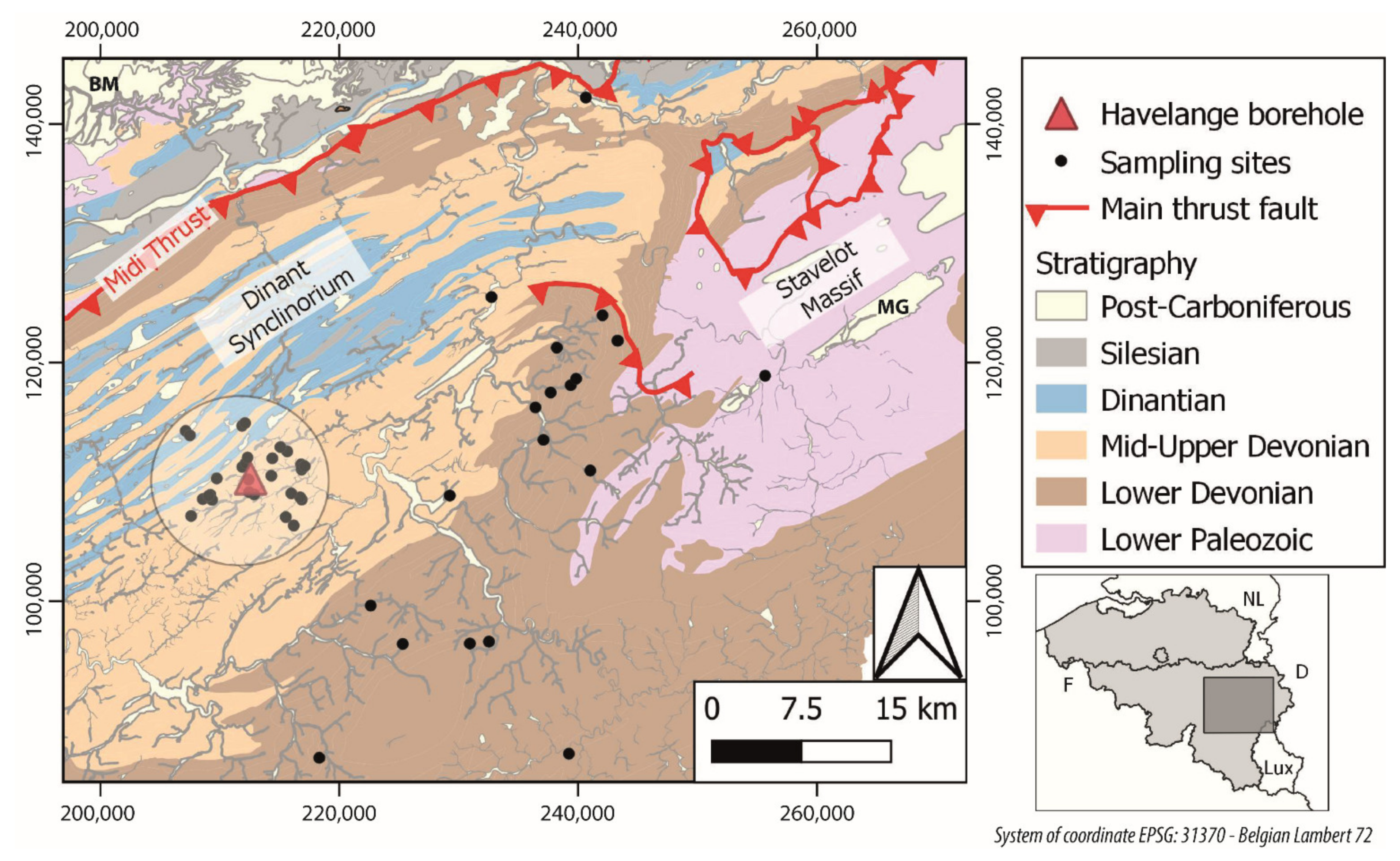
The study area and the Havelange borehole are located on the Eastern part of the Dinant Synclinorium, a sub-unit of the Ardenne Allochthon. These units compose the Belgian segment of the Rhenohercynian fold-and-thrust belt, which results from the accretion of the Rhenohercynian passive margin during the Variscan orogeny between the end of the Visean age to the Upper Carboniferous period (330–300 Ma) [17,18,19,20]. The Dinant Synclinorium (Figure 1) is bordered to the North by the trace of the Midi Thrust, which separates the Ardenne Allochthon from the Brabant Parautochthon [21].

The main lithologies composing the Dinant Synclinorium are thick detrital Devonian formations combined with carbonate formations of Givetian, Frasnian, and Dinantian ages. These Devono-Carboniferous formations underwent during their evolution high diagenetic conditions and even green-schist facies conditions for the deepest formations (Lower Devonian) [22].

The Dinant Synclinorium passes eastward to the Lower Palaeozoic Stavelot Massif inlier. The contact between the metasedimentary units of the Stavelot Massif and the Lower Devonian formation of the Dinant Synclinorium is marked by an unconformity reflecting the action of a branch of the Caledonian Orogeny. The rock of the Stavelot Massif underwent, therefore, the Caledonian and Variscan orogenies.

The main faults in the region are South- to South-East dipping longitudinal thrust faults, as well as bulged faults forming the Theux and Gileppe windows to the North of the Stavelot Massif [23]. The fold structures are oriented NE-SW or even E-W depending of local conditions. Transversal or oblique faults crosscutting the folds and longitudinal thrust faults were formed either at the end of the Variscan orogeny or even during the poorly controlled age post-Variscan events. Some of these transversal and oblique fractures were filled by significant Pb-Zn deposits. Other transversal fractures are frequent targets as conduits for superficial groundwater resources, especially in carbonate formations.

Since the end of the Variscan orogeny, the tectonic activity in the study area has been quite limited. In the Stavelot Massif, the narrow Malmedy graben was formed, probably during the Permo-Triassic period. The whole region underwent a global uplift during the Quaternary. The current seismic activity in Southern Belgium is mainly located along the rim of the Brabant Parautochthon and in the Stavelot Massif [24]. Only a very limited number low magnitude events (Local Magnitude (ML) < 3.0) were recorded in the study area and the probabilistic model for a return period of 475 years predicts a maximum ground acceleration ranging between 0.04 and 0.06 g.

Following its geological characteristics, the Havelange borehole was selected in the framework of the H2020 MEET project as a demo-site to evaluate the geothermal potential of EGS development in a setting of Variscan meta-sedimentary units not affected by a younger extension period.

The Havelange borehole [16] was drilled for the Geological Survey of Belgium between January 1981 and November 1984 and reached a depth of 5648 m (MD). It aimed to investigate the potential natural gas resources under the Midi Thrust and, therefore, to drill through the Dinant Synclinorium to reach the deeply rooted Brabant Parautochthon southern extension. The site selection for the Havelange borehole results from the gas detection in another deep borehole (Focant) and the results of a seismic reflection campaign conducted in 1978. This seismic campaign indicates the presence of deep bulge-like reflectors interpreted as the presence of a local dome of the southern extension of the Midi Thrust. The methane gas inflows were too limited for any economic development program.

Briefly, the Havelange borehole encountered from top to bottom:

• Micaceous sandstone, siltstone, and shale units of the Famennian age;
• Frasnian and Givetian limestone, dolomite and shale formations;
• Sandstone, siltstone, slate-phyllite, and quartzite thick bed of the Eifelian, Emsian, Praguian, and Lochkovian stages.

The borehole allowed the detection of several thrust faults indicated by the repetition of stratigraphic units especially in the lower part of the borehole.

The main mineralogical phases encountered are: quartz > illite/muscovite > clinochlore > calcite > dolomite > pyrophyllite > feldspar > garnet > hematite > ilmenite, with obviously major variations according to the lithostratigraphic units. Another important property to mention is the high level of lithification of the studied formation. Even if Rhenohercynian fold-and-thrust resulted from the accretion of sedimentary basin, the involved lithology underwent a major lithification, reducing the porosity to a few percent and, hence, the connate water content is more likely very limited. This context differs, therefore, significantly from oil-gas sedimentary basins associated with significant brine contents.

The study area was the object of several studies to evaluate the subsurface temperature and heat flow conditions at a regional scale. The temperature values recorded in the Havelange borehole frequently serve as input data to calibrate the models [16].

Vandenberghe and Fock [25] reviewed the existing temperature measurements in wells from Belgium. They established a series of temperature distribution maps for a set of depths. They observed some trends such as the presence of a cold anomaly located in the northern part of the Stavelot Massif, while high temperature halos (~40 °C/km) are present in Western and Northern Belgium. According to their study, the Havelange borehole is located in an average geothermal gradient zone. The main limitation of such maps is that isotherms are based on widely spread data from boreholes separated to each other by a few tens of kilometres. The determined isotherms are extrapolated on a large scale without taking in consideration any thermal parameters. As a result, the isotherms are smooth and obliterate the presence of any potential thermal anomalies at a local scale (few km).

More recent approaches applied 2D numerical models to compute the subsurface temperature and the surface heat flows again at a regional scale. These studies [26,27] consider the thermal properties (i.e., thermal conductivity and radiogenic heat production) and other parameters such as the density and porosity from reference rock samples or from published data for crustal horizons located at great depth. These models also rely on a selection of published deep cross-sections to establish the structure and the composition of the upper crust. The comparison of the works of Rogiers et al. [26] and Schintgen et al. [27] is a complicated exercise since the models follow very different numerical approaches and try to answer different scientific questions. Rogiers et al.’s. [26] study aims to understand the presence of low heat flow anomaly detected in the shallow part of some boreholes in Belgium (Soumagne, Grand-Halleux, and Havelange). They consider the influence of groundwater flow at a shallow depth through various heat transfer mechanisms: conduction vs. heat advection. The influence of Quaternary paleoclimate changes is also applied through temperature variation of the model top boundary condition leading to a transient model. The lower part of the model is associated with a homogeneous and constant heat flow at depths ranging from 20 to 10 km. In the case of the Havelange site, the estimated basal heat flow would be 90 mW/m² at 14 km deep.

By contrast, the model by Schintgen et al. [27] aims to evaluate the heat flow with a specific focus on the situation in the Great-Duchy of Luxembourg, but the studied sections extend to the Stavelot Massif and in the neighbourhood of the Havelange borehole. Their model is a 2D steady-state conductive model. The model dimensions are also very different, since the lower boundary condition correspond to lithosphere–asthenosphere boundary (LAB) located at a depth ranging from 80 to 130 km and with a temperature of 1300 °C. The model of Schintgen et al. [27] also consider the presence of an Eifel plume in Germanym resulting in a LAB depth reduced between 40 and 60 km. The lateral extension of this plume would reach the Eastern border of Belgium [28,29]. The model results evaluate the heat flow at 1 km deep in the South-East part of the Dinant Synclinorium to a value of c. 80 mW/m², while in Rogiers et al. [26], the heat flow at a shallow depth of the Havelange borehole is smaller, c. 55 mW/m². This low value would result from a downward water flow at a shallow depth in the Havelange borehole. Besides the numerous differences between the approaches of Rogiers et al. [26] and Schintgen [30], both modelling predict significant heat flow variations at a local scale in the shallow part of the studied areas. In the approach of Schintgen et al. [27], these variations result from strong thermal conductivity contrasts observed for the rocks composing the upper crust, whereas the forced water advection in the shallow crust is the driving mechanisms of Rogiers et al.’s [26] model.

Recently, a review work on the origin of CO₂ content of Fe-rich soda springs, mainly located in the Stavelot Massif, indicates that the water is of meteoritic origin, but the CO₂-content results from the mixing of sources from hypothetic carbonate dissolution and from magmatic origins [31]. Their study focuses mainly on the isotopic signature of H, O, C, and He. The CO₂ magmatic source is regarded by Barros et al. [31] to be linked to the Eifel plume.

Most of the previous models rely on old observations acquired during the 1960s and 1980s, thanks to the exploration deep well campaigns led by the Geological Survey of Belgium. Some debate points between models result frequently because of the very limited numbers of information. An example of this issue is the use of a specific cross-section as a base for the numerical thermal models. However, these cross-sections are matter of debates and the choice of another section will fundamentally modify the results of the numerical models.

The approach followed in our paper aims to acquire new information using a cost-effective approach for the geothermal exploration thanks to the geochemical analyses of spring waters. The collected samples were acquired in two distinct regions. A first group of water samples was collected in a 5 km perimeter around the Havelange borehole head. The subsurface composition of these springs is considered very similar to the geological formations observed in the shallow part of the borehole, that is, the mid- and upper-Devonian geological formations. This zone is referred to here as the “near field”. The second group of samples were mainly acquired in the South and East borders of the Dinant Synclinorium where mid- and mainly lower-Devonian formations outcrops. The analogue formations were encountered in the deep part of the Havelange borehole. This second sampling zone is named, here, “the far field”.

3. Materials and Methods

3.1. Sampling Campaign

The sampling campaign started with an initial deskwork phase for selecting potential target sites. This pre-selection includes the analysis of topographic, geological, and hydrogeological maps. A series of priorities were established based on the spring elevation, their position in a valley (e.g., lower part of the valley bank or at the valley head) or their vicinity with a fault. Springs located at an elevation lower than +250 m (Z) were considered as a priority, since this elevation corresponds to the static level of the Praguian and Lochkovian aquifer(s) in the non-cased section of the Havelange borehole. A site in the village of Moressée was also selected based on the toponymy of a spring: “La chaude Fontaine” (translated in English by “the hot fountain”).

An additional site located at the north end of the study zone in the city of Chaudfontaine was chosen to collect a reference sample of hydrothermal water. The natural mineral water source (Source Astrid) captured in the Frasnian limestone at a depth of 396 m reaches a temperature of 36 °C.

The 50 samples were collected and conditioned by the team of the Geological Survey of Belgium (GSB) between the 13 November 2019 and the 5 March 2020. The ISO 5668–11 recommendations and the OFEFP guide [32] were followed during the actual water sampling. Each site was also the object a detailed description regarding its environment, its precise location, the water flow magnitude, the presence of infrastructures (e.g., metallic pipes, concrete walls, etc.). Physicochemical parameters of spring water (pH, EC, T) were also measured in each site using a multiparameter meters from Hanna Instruments.

During the field campaign, some of the pre-selected sites were not sampled as some springs were dry. The region underwent a series of drought periods especially during the three previous summers. Conversely, the field reality led us to samples other sites discovered during the campaign.

All the observations, field measurements, and analytical results were included in a relational database designed for this campaign. A total of 20 samples were collected in the far field study zone and 30 samples in the near field. A table with the data used in this article are retrievable in Supplementary Materials (Table S1).

3.2. Laboratory Analyses

The central laboratory of the “Société Wallonne des Eaux (SWDE)” performed the analyses on the water spring samples on behalf of the GSB. The following parameters were measured: pH, electrical conductivity at 20 °C (EC), colour (ISO 7887 (C Method)), turbidity (NTU) (nephelometric method), dry residue (TDS), and suspended solids (SSC) (ISO 11923).

The major and minor anions (SO₄²⁻, Cl⁻, NO₃⁻, o-PO₄³⁻, NO²⁻, F⁻, Br⁻) were analysed by ion chromatography methods (ISO 10304-1, ISO 10304-4). The major and minor cations (Na⁺, K⁺, Ca²⁺, Mg²⁺, Ba²⁺, Fe (total), U, Mn⁺, Si⁴⁺, Sr²⁺), trace metals (Ag, Al, As, B, Be, Cd, Co, Cr, Cu, Hg, Li, Mo, Ni, Pb, Rb, Sb, Se, Sn, V, Zn) on unfiltered and filtered water were measured by Inductively Coupled Plasma Mass Spectrometry (ICP-MS) (ISO 17294-2). The concentrations of NH₄⁺ and the complete alkalimetric strength (TAC) were analysed by Spectrophotometry.

Other parameters such as the Total Hardness (TH) and the TOC (Total Organic Carbon) (ISO 8245) were also acquired. The presence and the distribution between HCO₃⁻/CO₃²⁻/dissolved CO₂ are deduced from the values of the Alkalimetric strength (TA) = (OH⁻) + (CO₃²⁻), the TAC = TA + (HCO³⁻), and pH. The details of the laboratory parameters and LOQ are presented in the additional material (Table S2).

3.3. Data Treatment Methods

The interpretation of the water spring analyses made in this paper is based on the filtered water results. The use of filtered water (filtration at 0.45 microns) allows to concentrate the interpretation on the dissolved element in water and avoid the micro particles present in non-filtered water (e.g., clay).

Before statistically processing the data, the charge balance equilibrium (CBE) of the analytical values of the 50 water samples (converted from mg/L to meq/L) were calculated, using the formula: (CBE(%) = ((Scat − San)/(Scat + San)) × 100; S, cat, and an mean total, cation and anion, respectively [33]. Applied on one hand to major ions only (those used for Piper Diagram) and on the other hand to major and some minor ions (those mentioned in annual report of SPW-Agriculture, Ressources Naturelles et Environnement: F, PO₄, NO₂–Sr, Ba, Al, Fe, Mn [34], the resulting CBE are ranging as follows: (0.02–9.89%) with an average of 3.47% for MAJOR and some MINOR ions of 49/50 water samples; only one sample with CBE > 10% sample 32 at 28.10%.

The Piper diagrams [35] and the Stiff diagrams (e.g., [36]) were also made in this unit of measurement. The total ionic salinity (TIS) with Na + K vs. Ca + Mg is expressed in meq/kg [37]. The nitrate concentration values due to potential anthropic contamination of the water composition, from superficial water samples especially, are not included in the Piper diagrams. Finally, a hierarchical clustering method was applied and specifics elements of hydrogeological or geothermal interest (Li, Rb, pH, NO₃, etc.) were selected to be represented as boxplots. In addition, several maps were made to show the locations of the clusters and the concentration in particular elements with the use of the Jenks natural breaks classification methods.

3.3.1. Hierarchical Clustering Methods

The geochemical analyses acquired during this campaign are the results of several cases of the water evolution during its subsurface transit. The latter can be short (e.g., superficial water in and out-flow during a brief period) or long (deep fluid circulation or shallow low-permeable system). The geological setting of each spring can also be influenced by numerous parameters, such as the mineralogical composition of the rocks and the specific dissolution rate of their mineral, the physicochemical parameters of water during its interactions with the minerals, amongst others. The mixing of water masses that followed different subsurface paths certainly represent a key factor influencing the spring water composition. Finally, external parameters influencing the spring water composition are the climatic conditions (rain precipitation regime) or possible natural or anthropic contaminations (e.g., mineral deposit interactions, road de-icing, or agricultural spreading). Hence, the challenge is to detect the key trends and key parameters allowing us to detect trends in a multivariate system. In this study, we have chosen to apply the hierarchical clustering method to discover a structure in the data set. The hierarchical clustering method was applied on all 50 samples and for a set 37 parameters, including the physicochemical parameters (e.g., pH, EC, TAC), the concentration of the major anions, and trace metal cations. The data set is organized in a matrix of 50 rows and 37 columns. In a first step, the Euclidean distance is computed between each row (i.e., sample) of the matrix in a m-dimension space, with m equals to 37. The output of this first operation is a distance matrix, which represents the input data for the hierarchical clustering. Concretely, the distance matrix and the hierarchical clustering were computed by applying the dist and the hclust functions from the base ‘Stats’ Package from the R language [38]. The hierarchical clustering outputs are commonly represented by a dendrogram where the distances between the samples is represented by a difference of height between the tree limbs.

3.3.2. Jenks Natural Breaks Classification Methods

The Jenks natural breaks classification method is used to create a map based on any kind of data with spatial attribute. This method conducts natural groupings (clusters) inherent to the chosen data (e.g., the concentration in one element). The breaks are determined to find the best group with similar values and with a marked difference between classes. This method pursued to minimize the variance within classes and maximize the variance between classes [39]. In the GIS application, the number of desired classes in a result set for the Jenks method must be added before the algorithm is applied on the dataset. In this paper, the reference separation was chosen at five, after different tests.

The Jenks method is applied in this study to create thematic maps based on the element concentration (Li, Rb and Sr) with QGIS software. It allows us to see the natural break in the concentration dataset for each element.

4. Results

4.1. Hierarchical Clustering of Water Analyses

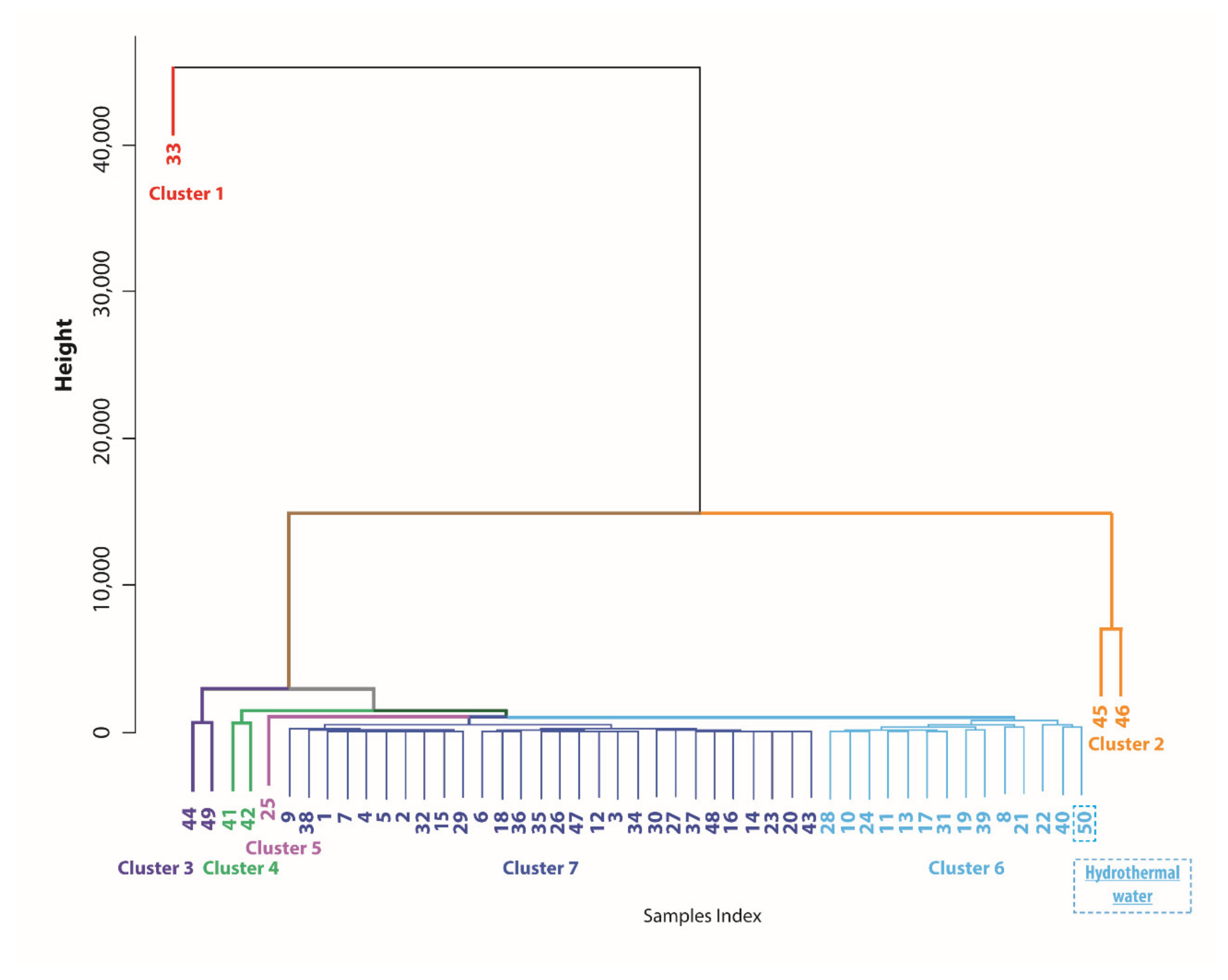
The application of the hierarchical clustering on the spring water dataset (Figure 2) indicates that seven clusters can be reasonably distinguished. Cluster 1 contains only one sample (n°33) collected in the lower Palaeozoic Stavelot Massif in the vicinity of the Permian graben of Malmedy. This sample in the dendrogram occupies its own limb with a significant distance with all other samples. Clusters 2 to 4 include two samples each, whereas cluster 5 has only one sample (n°25). As we move down in the dendrogram, the height between the limbs is decreasing, reflecting tighter clusters or, in other words, samples with compositions more and more similar. The last two clusters (6 and 7) include 14 and 28 samples, respectively, and encompass the bulk (84%) of the collected samples.

In this analysis, the hydrothermal reference sample (n°50) from Chaudfontaine is classified within cluster 6 along with 13 other samples, which show, therefore, a degree of affinity in their chemical composition with the hydrothermal reference one. A corollary of this observation is that the composition of samples from clusters 1 to 4 clearly deviates from the bulk of collected samples and from the hydrothermal reference sample. At this stage of the analysis, the results indicate that in terms of anomalies, the study area is, thus, characterized by several types of springs with “abnormal” compositions.

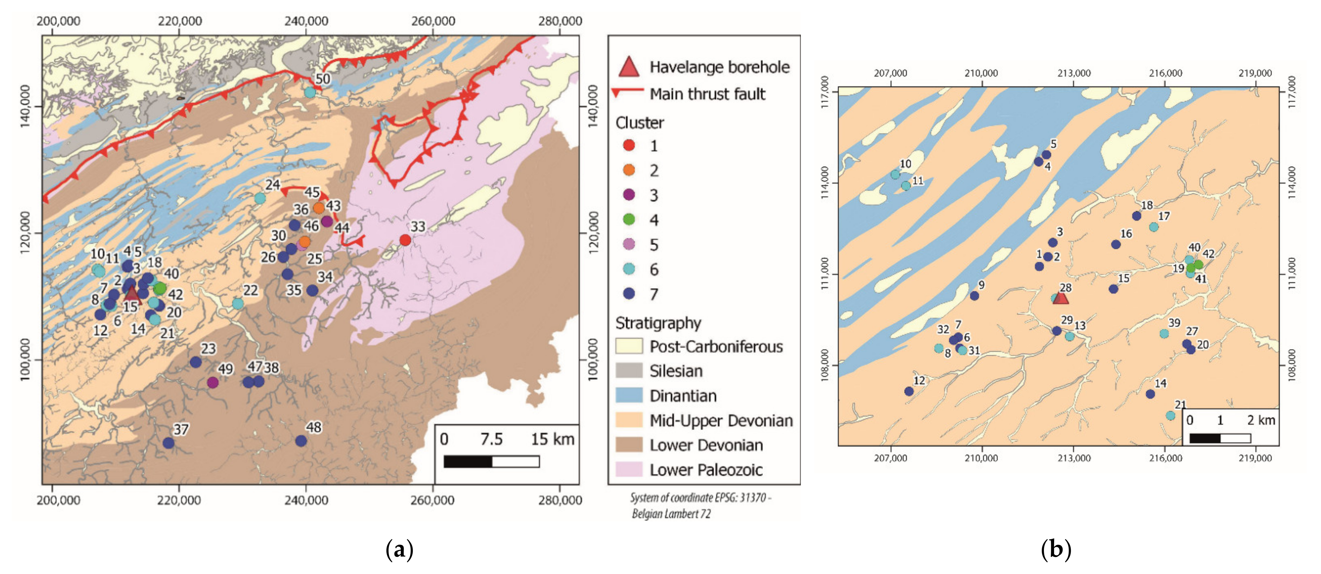
The samples from clusters 1 to 3 and cluster 5 (Figure 3) come from sites located in the Stavelot Massif and mainly the Eastern rim of the Dinant Synclinorium, which is the study zone “far field”. In this region, the surface and subsurface formations consist primarily of Lower Palaeozoic and Lower Devonian detrital meta-sedimentary rocks (phyllite/slate, sandstone, and quartzite). By contrast, samples from cluster 4 originate from a very limited zone located 4 km to the East of the Havelange borehole site. The samples of cluster 6 were collected mainly in the near field with two other samples located on the west edge of the far field. As already stated, the reference hydrothermal water from Chaudfontaine is located at the north end of the study zone. Finally, the samples of cluster 7 cover indiscriminately the entire study zone with a common characteristic of a low salinity (TDS ranging from 46 to 276 mg/L and TIS < 9.25 meq/kg (see Figure 8 in point 4.3).

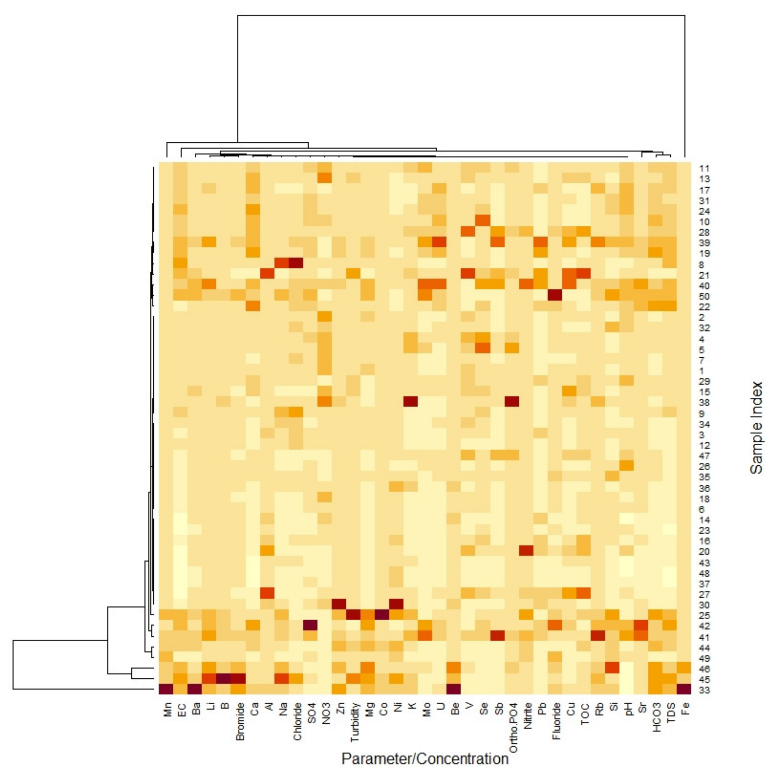
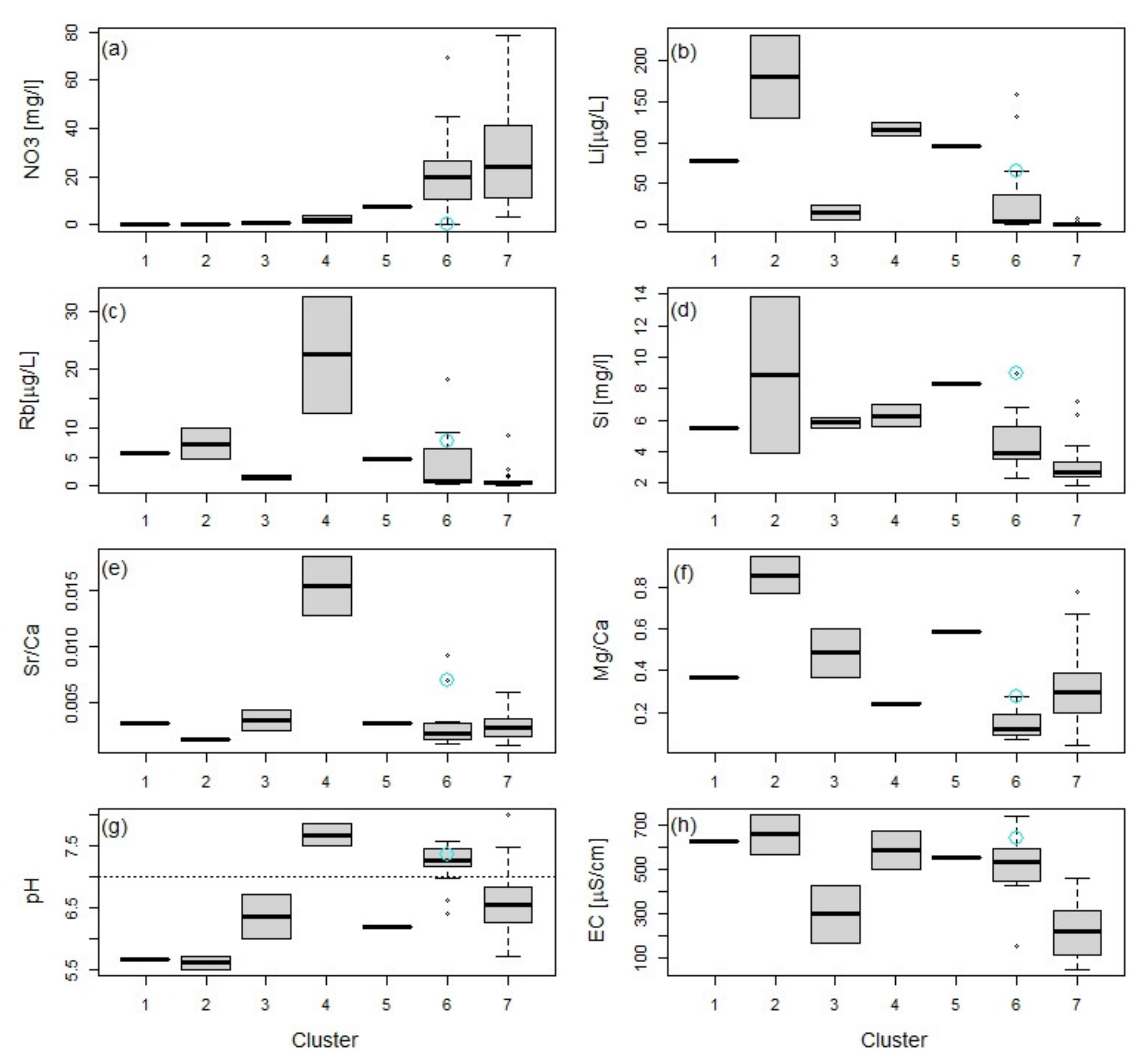
4.2. Heat Map and Boxplots

Even if the hierarchical cluster provides valuable information to detect compositional affinities/dissimilarities between samples, it does not directly provide the key compositional characteristics of each cluster. Regarding cluster 1, the examination of laboratory results indicates a very high concentration of iron (45,052.0 mg/L) and manganese (4321.3 mg/L), while the mean iron concentration for the dataset reaches 1462.7 mg/L and 189.5 mg/L for manganese and the median values are only 5 mg/L for Fe and 1.25 mg/L for Mn.

For the other clusters, the set of elements characterizing them is less obvious to detect. Figure 4 presents a heatmap on the same dataset as for the hierarchical clustering. Note that parameter values or concentrations for each column are normalized to avoid the predominance of very high values (e.g., iron or manganese concentration) with respect to lower values as those of trace elements. The study of the heatmap indicates three broad horizons of values. From bottom to top, one can distinguish a lower horizon gathering samples from clusters 1 to 5 that are characterised by high concentration of numerous elements, such as Fe, Mn, Ni, Be, Mg, Li. These samples have usually a low concentration of NO₃, Se, Sb. The EC and TDS are usually high, and the pH level is variable. Some sub-horizons can be distinguished with for instance the samples from cluster 4 (sample n°41 and 42), which show higher levels of Sr, Mo, and Sb. The central horizon of the heatmap (from samples 30 to 2 along the sample index axis) contrasts with, globally, a low concentration in several elements: Li, Rb, Ca, Na, K, Mo, U, HCO₃. These low levels are also reflected by low EC and TDS values. At least a part of these samples is also affected by high nitrate levels. This central horizon is occupied by samples from cluster 7. Finally, the top heatmap horizon, which corresponds to cluster 6, shows, again, higher levels in numerous elements, but not the same as in the lower horizon. The high levels of the top horizon include Bromide, Mo, U, V, Se, Sb, Cu, TOC. The EC, TDS, and pH levels are usually higher than in the central horizon.

The high nitrate levels from spring water in areas with intense agricultural activities such as in the study area are commonly regarded as a signal of anthropic contamination of the aquifers. For our study, we can consider that high NO₃ levels is a good indicator of important influx of superficial water within the aquifers drained by the springs. Clusters 5 to 7 (Figure 5a) gathers, therefore, springs with water from superficial flow or at least a mix of superficial water with deeper aquifers. Interestingly, the water from Chaudfontaine well occupies the minimum quartile (Q1) of cluster 6, indicating the absence of any significant nitrate input in this hydrothermal system.

Li, Rb, and Si are amongst the numerous elements that are commonly analysed to detect and to characterize the presence of geothermal water. In our dataset, the higher levels of lithium (Figure 5b) are observed in Clusters 1, 2, 4, 5, and the upper part of cluster 6. By contrast, water samples from cluster 3 and mainly 7 are lacking significant Li concentrations. A similar observation can be applied for the Rb concentration (Figure 5c). Even if the Li and Rb levels observed in cluster 3 are quite similar with those of clusters 6 and 7, the Si concentration of samples from cluster 3 is clearly larger than in the other two clusters (Figure 5d).

Element level ratios are also frequently evaluated to characterize the aquifers, such as [Sr]/[Ca] and [Mg]/[Ca] (Figure 5e,f). The results indicate that cluster 4 is characterized by high values of [Sr]/[Ca] with respect to all other clusters, while it is more difficult to detect a clear trend for the ratio [Mg]/[Ca].

The analysis of the pH levels (Figure 5g) shows that water from clusters 4 and 6 is mainly composed by water with a pH above 7, while the other clusters are primarily associated with slightly acidic water. Finally, the EC of clusters 1, 2, 4, to 6 have high values, while clusters 3 and 7 exhibit low or intermediate electrical conductivity (Figure 5h).

4.3. Water Composition

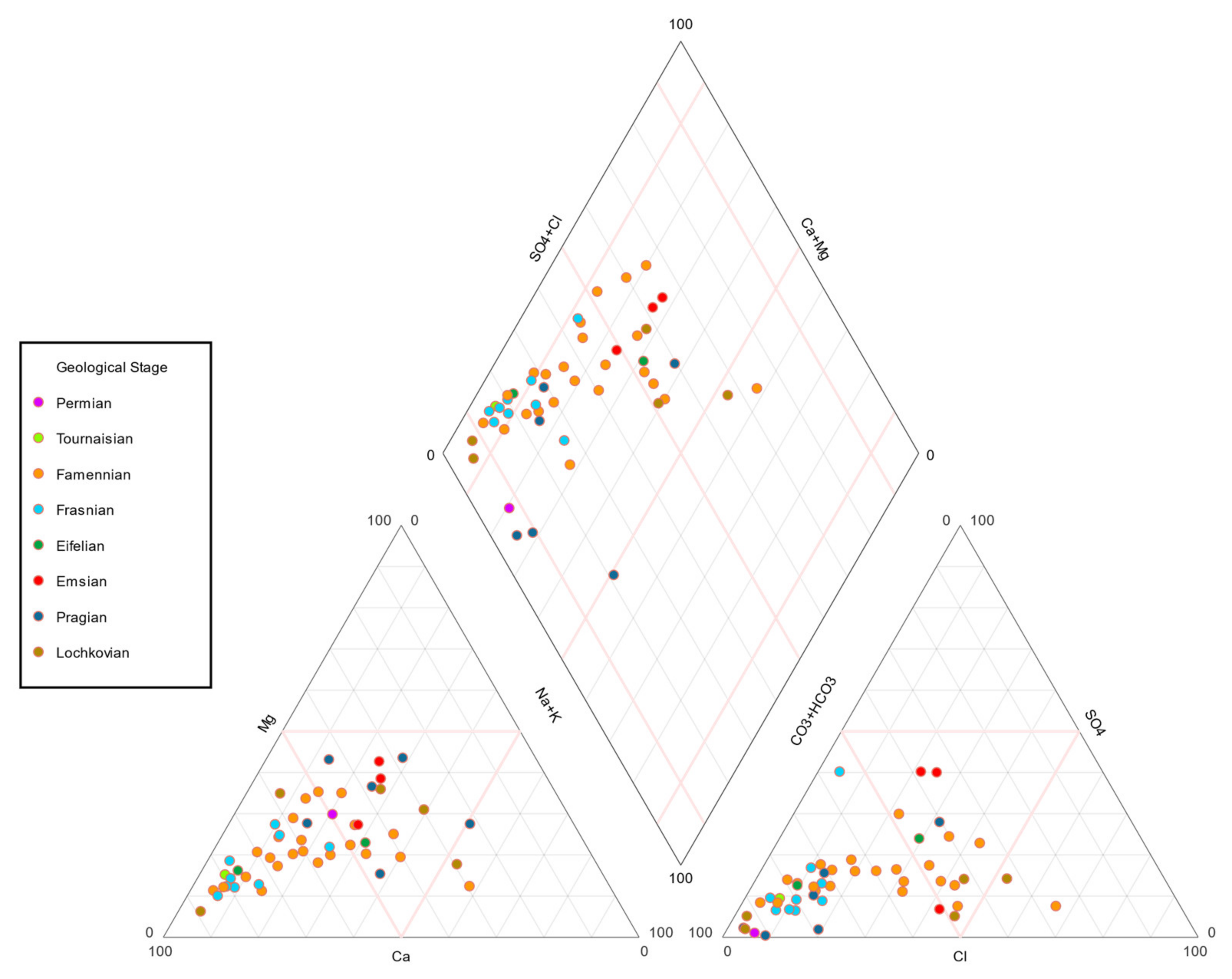
The Piper diagram of the filtered samples (Figure 6) shows that 86% of the spring water samples can be classified into three main categories, namely the “Magnesian Calcium”, “Calcium and Magnesian bi-carbonate”, and “Chlorinated and sulphated calcium and magnesian” types. It is observed that the samples rarely belong to a type containing high concentration of sodium and none of them are of “magnesium” type or in “sulfate” type.

A total of 23 water samples were collected from sites where the Famennian detrital formations outcrop. Their major dissolved constituents exhibit a broad spectrum of compositions, including the three aforementioned main water types (i.e., Ca + Mg, Ca(Mg)HCO₃ and Ca(Mg)Cl(SO₄)). The dominant cation is Ca or there is no dominant cation, whereas the bicarbonate anion is dominant or no dominant anion can be identified. The nine samples from the outcropping zone of carbonate and shale formations of Frasnian age are characterized by a composition of mainly Ca + Mg type with Ca and HCO₃ as the dominant ions. The three samples from Emsian formation indicate a sulphated composition.

The Praguian meta-sedimentary rocks (phyllite, siltstone, sandstone, and quartzite) are of great interest in this study since they represent the main target for the geothermal development of the Havelange demo-site and they represent a cumulative apparent thickness by tectonic staking of 1565 m in the borehole. The six spring water samples from the Praguian Stage show a much broader distribution of compositions with bicarbonate as the main anion, but without any dominant cation. However, three samples from the Praguian and one from the Permian are located on the lower triangles (Na-K-HCO₃ type). This type can indicate a cation exchange (Na, Ca) carried out by a deep-water circulation over a long period in clay facies. It is hazardous for the other Geological Stages to detect a clear trend or to evaluate the composition coverage due to the very limited number of samples per stage.

This broad distribution of compositions and their rather weak relationships with the Geological stages reflect the difficulty to associate the composition of a spring water with its surface geology. As we will discuss in the following parts of this paper, numerous springs discharge superficial water masses with a short subsurface transit period from the recharge zone and without enough time to reach a real equilibrium with their host rocks. On the other hand, water volumes flowing from deep units are likely to be in contact with several formations of different lithologies. The attempt to link the spring water composition of the main elements with the surface geology must be regarded as an oversimplification.

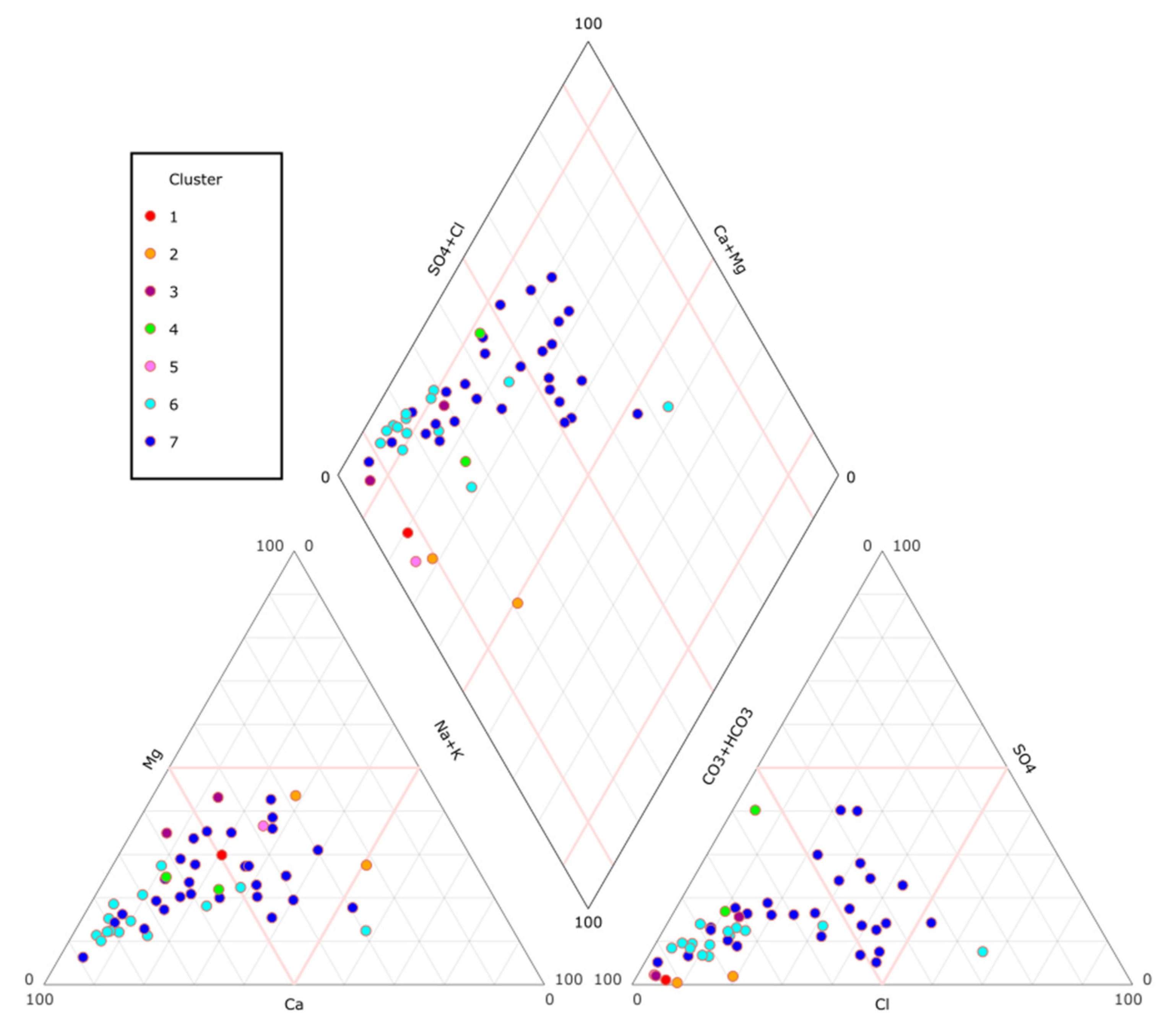
The second Piper diagram represent the 50 water samples according to the defined clusters (Figure 7). For samples from clusters 1 to 5, it is not possible to define a trend due to the very limited number of samples per cluster (e.g., 1 or 2). However, samples from clusters 1, 2, and 5 are located close to perimeter of HCO₃ + CO₃ type water. By contrast, many samples from cluster 6 are located along the Ca + Mg water type or within the Ca(Mg)HCO₃ domain. Finally, the water samples for which there is an indication of superficial subsurface flow (cluster 7) spread over a broad zone, including Ca(Mg)HCO₃ and Ca(Mg)Cl(SO₄) water types.

If we compare the Piper diagram of surface geology (Figure 6) with the one of clusters (Figure 7), two relationships can be detected. First, the spring water samples collected from sites where the surface geology belongs to Famennian formations are frequently attributed to cluster 7, namely the group of superficial waters. This relationship indicates that the shale formations of Famennian age act as aquiclude leading springs discharging only very superficial water masses. A corollary of this statement is that the same shale act as a cap rock for the deeper water masses. The second relationship is indicated by a degree of correlation between water samples from cluster 6 with samples collected in the outcrop zones of the Frasnian carbonate and shale formations.

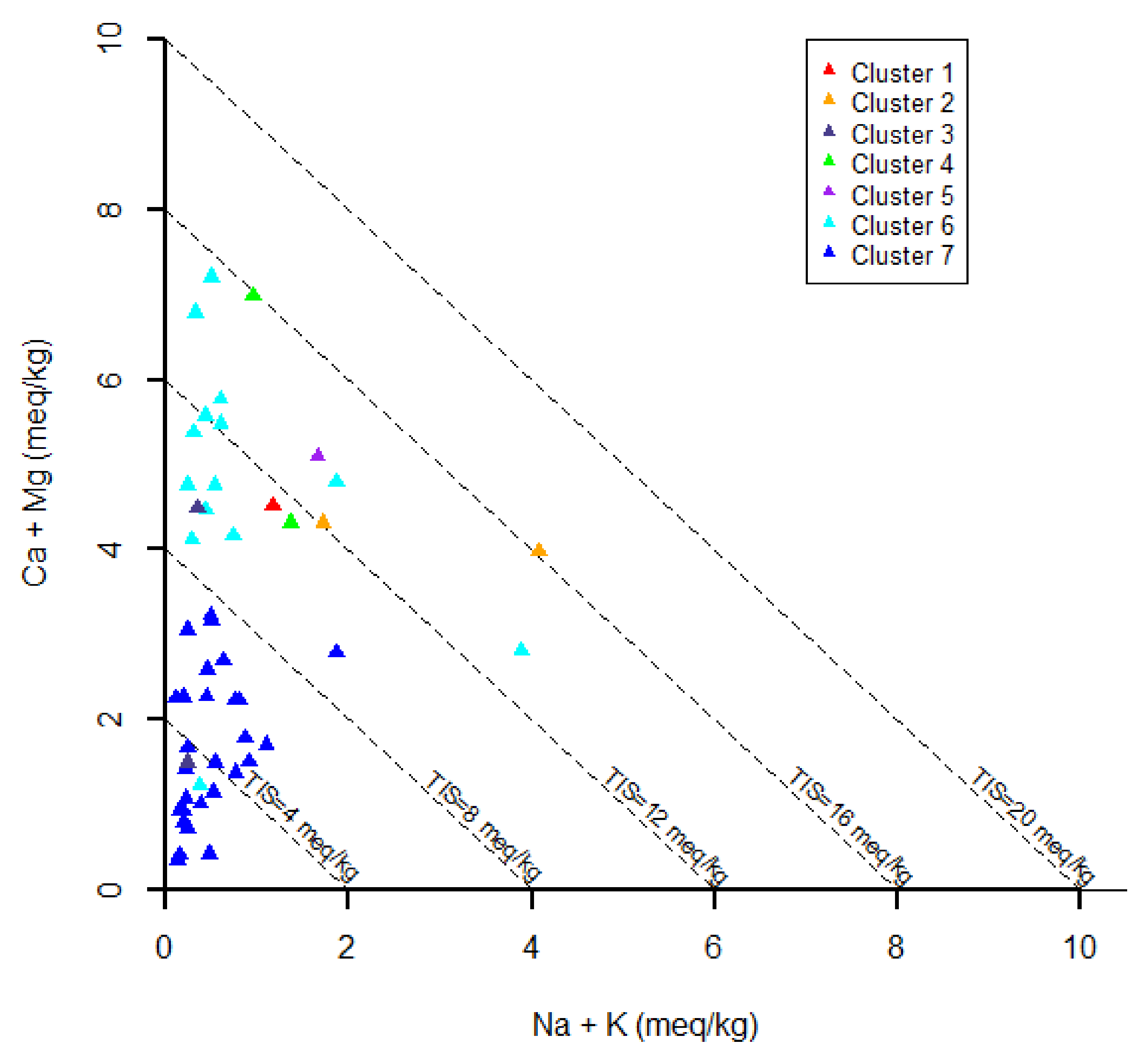
Furthermore, the spring waters show low total ionic salinity (TIS) values between 1 and 16.25 meq/kg (Figure 8). More specifically, the lowest TIS < 9.25 meq/kg are associated with cluster 7 (identified as superficial water). All the other samples, except one from cluster 6, have a TIS > 9.25 meq/kg. In addition, cluster 6 (which contains hydrothermal water) presents a higher concentration in Ca + Mg than in Na + K. On the other hand, one sample from cluster 2 and one from cluster 6 show higher concentrations in Na + K than in Ca + Mg.

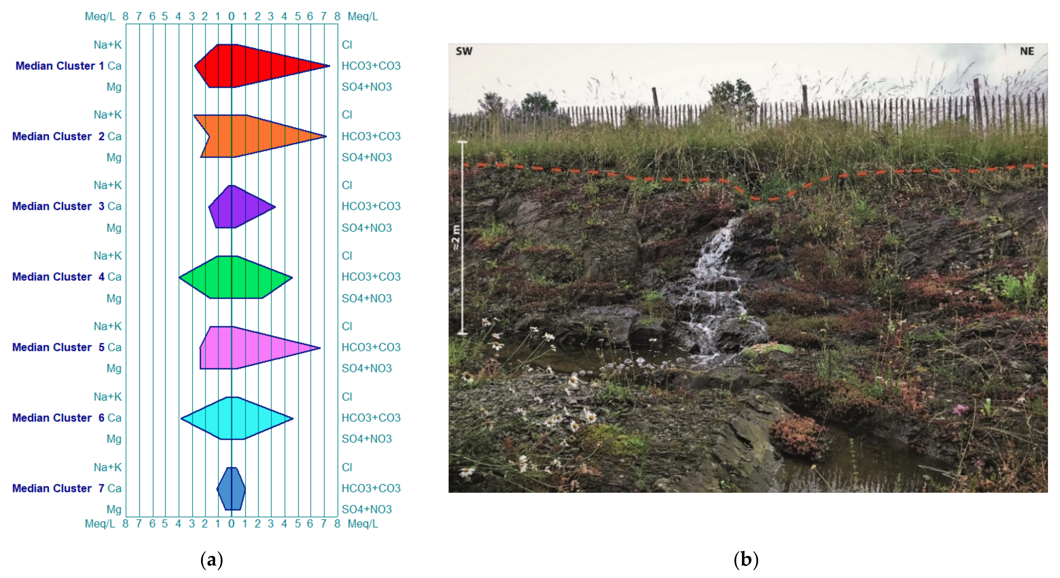
4.4. Stiff Diagrams and Clusters

The Stiff diagrams presented in this paper are built with the median values of the main constituents from each cluster expressed in meq/L (Figure 9).

The clusters 4 and 6 are the ones that show the most typical shapes for bicarbonate calcic groundwaters. However, cluster 4 shows enrichment in SO₄ compared to cluster 6. The clusters 1, 5 (one sample each), and the cluster 2 are characterised by an asymmetric polygon due to an elevated concentration of bicarbonate (around 7 meq/L) in comparison to cluster 4 and 6. This might reflect a deeper source of CO₂ in these waters. Moreover, cluster 2 shows a relative depletion of Ca compared to Na + K and Mg. This probably reflects the occurrence of cation exchange processes affecting groundwater, which has circulated deeper, in contact with clay materials. Cluster 3 presents intermediate mineralization with low indication of anthropic contamination (low Na, Cl and NO₃). This might be the result of groundwater circulation through geological units that contain a relatively low level of potassium. Finally, the cluster 7 displays the lowest global mineralization, reflecting surface waters or very shallow groundwaters.

The Stiff diagrams of all the samples are available in additional material (Figure S1).

4.5. Anomalies and Elementary Maps

The previous heatmap (see Figure 4) highlights three main horizons in the dataset. Each horizon reflects a group of samples with similar constituents’ concentration and/or similar physicochemical parameters. At the scale of a single sample the concentration in a specific element can be regarded in some cases as an anomaly within its heatmap horizon. Sample n°5 has for instance a higher Se level with respect to all other samples in the central heatmap horizon. Such deviation from the trend/horizon, that is an anomaly, can result from a water transit through a specific subsurface environment such as the presence of mineral concentration. The evaluation of anomalies in the composition of water can be conducted in different ways. For this study, the first approach consists of the application of the Jenks natural breaks with five classes for a set of 16 elements. A sample is considered with anomalous concentration in a given element if its concentration belongs to the two upper Jenks classes.

Table 1. Summary table of samples showing anomalies (higher than the Jenks mean concentration value for each chemical element).

Sample	Cluster	Element																Total
		Li	B	Si	Mn	Fe	Co	Ni	Cu	Zn	Br	Rb	Sr	Mo	Ba	Pb	U
10	6																X	1
11	6													X				1
15	7								X									1
17	6																X	1
19	6															X	X	2
21	6								X							X		2
22	6												X					1
25	5		X	X	X		X	X		X								6
27	7								X									1
30	7							X		X								2
33	1		X		X	X	X			X	X				X			7
35	7			X														1
36	7							X										1
39	6	X		X					X			X		X	X	X	X	8
40	6	X							X				X	X	X	X	X	7
41	4	X	X									X	X	X				5
42	4	X		X								X	X	X				5
44	3				X			X		X								3
45	2	X	X		X	X	X	X			X							7
46	2	X		X	X	X				X	X							6
49	3				X													1
50	6		X	X							X		X	X	X			6
Total		6	5	6	6	3	3	5	5	5	4	3	5	6	4	4	5

presents the results of detected anomalies.

Nearly half (22) of the collected samples exhibit a least one element with a concentration anomaly. In this analysis, samples n°39, 33, 40, and 45 show the highest number of anomalies and the elements reported more frequently as anomalies are Li, Si, Mn, and Mo.

Surprisingly, some anomalies are detected even in samples related to superficial water (cluster 7). The explanation for those particular cases are not easy to address, but at least in one case (sample n°15), its copper anomaly can be linked to the presence of a former Pb-Zn-Cu mine near the village of Heure [40,41].

Another approach to evaluate the presence of abnormal compositions is to compare the measured concentrations with literature values of element concentration in aquifers. For instance, six samples in the dataset have a Co concentration > 0.33 µg/L, which is a level well above the average value generally reported for spring waters [42]. In the same way, five samples have a Ba concentration > 100 µg/L [43] and seven samples have a concentration Mn > 200 µg/L [44]. In this paper, the focus is made on Li, Rb, and Sr concentrations in the water spring samples (Figure 10).

4.5.1. Lithium

The concentration of lithium in fresh waters usually ranges between 1 µg/L and 20 µg/L [45]. In this study, 11 samples (

Table 2. Table of MEET samples with the concentration Li, Sr, Rb: [Rb] > 7.6 µg/, [Li] > 20 µg/L or [Sr] > 1000 µg/L.

Sample n°	17	25	33	38	39	40	41	42	44	45	46	50
Li (µg/L)	36.6	96.4	78.5		131.6	158.9	123.8	107.6	23.3	229.9	129	65
Rb (µg/L)	9.3			8.6	18.4		32.6	12.5		9.9		7.6
Sr (µg/L)							1110	1280

) have a concentration of Li above 20 µg/L. Lithium deposits or concentration are usually found in salars or in pegmatites and less frequently they are found in clays and Li-rich micas. There is no observation of salars or pegmatites in the region and, hence, the Li source comes probably from clay minerals. However, mineral occurrences of Lithiophorite ((Al,Li)MnO₂(OH)₂) with possible traces of Co, Ni, Cu, and Zn are reported in the mines of Rahier, Bihain, Vielsalm, and Malempré in the Stavelot massif. No similar occurrence has been reported so far in the Devonian formations. One of the hypotheses is that the high concentration of lithium in the MEET samples could come from deep fluids that crossed Devonian formation.

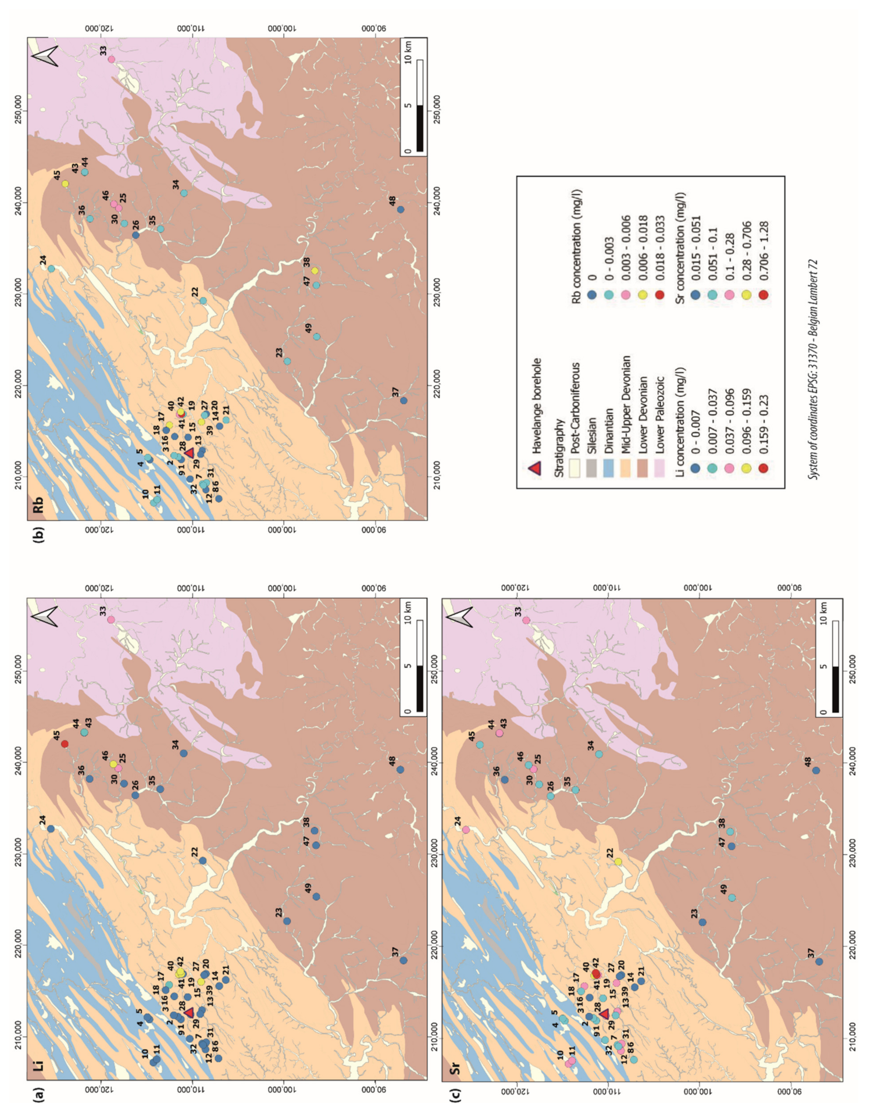
4.5.2. Rubidium

Rubidium is usually found in potassium minerals such as lepidolite, biotite, and feldspar. In natural groundwater, the Rb concentration is around 0.1 to 100 µg/L [46]. In this study, all the samples are below the highest reference values for spring water 100 µg/L. The referential sample n°50 (hydrothermal spring) shows only 7.6 µg/L of Rb. Six samples are above the referential sample n°50 and three of them (samples n°42, n°39, and n°41) are higher than 10 µg/L (Table 2). Four sampled sites are located in the near field (samples n°17, n°39, n°41, n°42) to the East of the Havelange borehole and two others are in the far field (samples n°38 and n°45). These samples are mostly located in shale, siltstone, and sandstone formations.

4.5.3. Strontium

Strontium enters into the groundwater composition during the leaching of limestone, igneous and metamorphic rocks, especially in granites and sedimentary rocks, as hydrated Sr²⁺ [47]. The concentration of strontium in fresh water is generally present as traces below 1000 µg/L [48]. The referential sample n°50 (hydrothermal spring) shows only 455.1 µg/L of Sr.

In the spring water from this study, two samples (n°41 and n°42) are above 1000 µg/L (Table 2). The high concentration of strontium for these samples could come from the leaching of Givetian or Frasnian limestone formations. Moreover, a strontium occurrence (Celestine) has been described in the literature near the village of Verdenne, on the East of Marche-en-Famenne city.

5. Geothermometry

One of the main goals of geochemical exploration through the evaluation of spring water composition aims to quantify or at least to estimate the thermodynamic conditions encountered by water during its path from the recharge area to the potential geothermal reservoir and in turn in discharge zone. Numerous equations are published to derive the geothermal reservoir temperature, but all these equations are based on a series of assumptions leading to a specific field of applications. This field of application includes some restrictions with the main ones that are the range of temperature values within the geothermal reservoir, the assumption that the thermodynamic conditions are satisfied for a reaction equilibrium between the water and the reservoir rocks, but also the geological setting (volcanic zone, sedimentary basin, metamorphic terranes…). The available papers on the subject usually discuss the field of applications, but even in these cases it is not always straightforward to decide if a particular equation can or cannot be applied. For instance, even if we have detected geochemical anomalies of subsurface water on the East side of the study near field, we must assume that the reservoir temperature fits with the temperature range of the applied geothermometers. For our study case, the temperature constraints within the Havelange borehole are known to be limited with a maximum bottom temperature of 126 °C (after correction) measured at 5369 MD (5277 m VD) [15]. Another temperature value is related to the Chaudfontaine site where the temperature of 36 °C was recorded during the sample collection, while for the other sites the spring temperature ranges between 3.7 °C and 14 °C. As a result, the geothermometers developed for the very high temperature conditions are not necessary the most appropriate for our study.

Some geothermometers were developed for geochemical reaction of minerals as feldspars, which are present in the Havelange borehole subsurface, but in a limited proportion. The available literature abounds with geothermometer evaluations for high-enthalpy geothermal systems in magmatic and volcanic contexts, but the number of geothermometer research in fold-and-thrust belt setting is quite limited. The closest domain of such evaluation to fold-and-thrust belt corresponds to sedimentary basins, with the main source of information on the reservoir water composition and temperature coming from oil fields. In this setting, the temperature ranges are usually quite low, but the conditions are not identical to those of fold-and-thrust. Amongst the differences the rocks of the Rhenohercynian Variscan orogen are strongly lithified, the diagenetic and metamorphic reactions are completed, and the porosity/permeability is mainly controlled by fracture networks, since the primary porosity is strongly reduced. From a lithological point of view, geothermometers were published by Chiodini et al. [49] for a geological setting, including limestone and evaporite formations. Their study led to a good correlation between a theoretical model and water samples collected in the Etruscan Swell (Italy). The occurrence of Givetian-Frasnian limestones in our study area could represent a promising target for the application of the Chiodini et al.’s model [49]. However, evaporite deposits were not recognized in the subsurface of the Havelange demo-site. Hence, our water samples are strongly undersaturated in SO₄ concentration (between 0.03 and 3.41 meq/L), which is between three orders of magnitude and at best a factor 3 lower than samples from the Etruscan Swell. This SO₄ deficit induces an overestimation of the reservoir temperature (~>100 and 150 °C) even for samples of superficial waters.

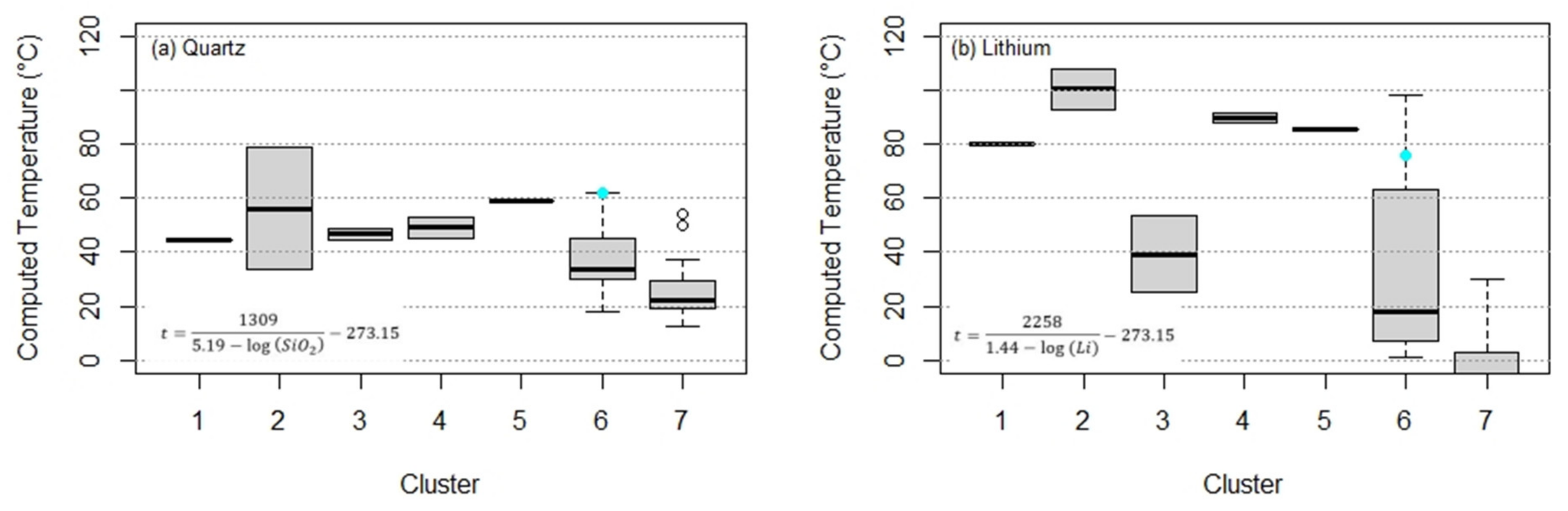
Despite these unknown parameters and uncertainties on the field of application of the geothermometers, we attempt and discuss some of the published geothermometers. The most widely used geothermometer is the one based on silica concentration in water. Different equations are available according to the silica forms [50]. It is usually considered that the quartz phase is controlling the silica dissolved concentration for water temperature above 180 °C, while chalcedony is the main phase governing the water silica content for a temperature below 110 °C. Between these values, the main controlling phase is undetermined. If we applied the equations developed by Fournier [50] for the dataset of this study, several problems are encountered: firstly, the ranges of computed temperatures for amorphous quartz, α-cristobalite, β-cristobalite include only negative temperature values. If chalcedony is considered as the controlling phase of dissolved silica, negative temperatures are computed for most of the superficial waters associated with cluster 7 of the hierarchical clustering. Some negative temperatures are also evaluated for samples of cluster 6. For the other cluster, the temperature values are quite small. Secondly, another problem in this approach is that the computed temperature for the Chaudfontaine hydrothermal reservoir is only 29.9 °C, while the recorded temperature at the sampling site is 36 °C. For similar reasons, Graulich [51] applied the equation of quartz and evaluate a temperature of 50 °C for the reservoir of Chaudfontaine. If we apply the equation for quartz to the dataset of our study, we can observe that the computed temperature values vary according to the clusters (Figure 11a). Computed values for clusters 1, 3, and 4 are located near a temperature of 50 °C. The two points belonging to cluster 2 exhibit different values: 33.5 and 79.1 °C. Cluster 6 corresponds to temperatures stretching between 17.9 and 62.0 °C. The last value equals the computed temperature of the reservoir of Chaudfontaine. Finally, the superficial water samples (cluster 7) are associated with the lowest temperature except two outliners.

The question of the application of the quartz phase equation for our dataset remains. It seems surprizing that the widely used silica geothermometers lead to unrealistic values if chalcedony is considered and if the quartz phase equation is applied the computed temperatures seem closer to conceivable values, but we apply an equation far below its lower temperature limit (180 °C) that is the equation is applied out of its field of application. Several remarks need to be addressed. First, Brook et al. [53] consider that in granitic massifs, the quartz is still the controlling phase for the dissolved silica down to a temperature of 90 °C. An assumption would be, therefore, to extend this lower limit even below 90 °C in the case of the rock assemblage like the one of Havelange in a setting of a fold-and-thrust belt, but the thermodynamic explanation will need to be addressed in the future. Another explanation of such paradoxical situation is that all silica geothermometers are directly related to the silica concentration. Hence, the unrealistic temperature observed with the chalcedony equation is related to abnormal low SiO₂ concentrations in the collected samples. In this case, the reasons of this SiO₂ apparent deficit are manyfold: the amount of chalcedony available for reaction with water in the Havelange subsurface is too small. Another possibility could be by the admixture of water with another water mass with a low SiO₂ concentration (e.g., superficial water). The water flow in the subsurface is too high to allow a full equilibrium between the water and the reservoir rocks. Finally, the potentially SiO₂-rich water in the near field that would flow at great depth are likely to encounter carbonate rocks during the ascending phase. The flow through the carbonate formations is likely to be associated with several reactions associated with the change in physicochemical conditions. The last two assumptions (fast flow, carbonate reactions) seem, however, unlikely since the abnormal computed temperatures are observed in both the near and far field. In this last zone, some of the geochemical anomalies are related to sites where the presence of limestone in the subsurface has never been recognized. Finally, the assumption of a fast-ascending flow is incompatible with the low temperature recorded in the springs.

The geothermometer analyses are rarely conducted with just one method, but it is common to compare the results of several methods. Another method based on a single element is associated with the Li concentration [52]. If applied on the Havelange dataset, it comes out that the computed temperature for clusters 1, 2, 4, and 5 are significantly higher than with the quartz geothermometer (Figure 11b). The computed temperature values for this group range between 80.4 and 108.3 °C. Cluster 6 includes values covering the full interval between 100 and 0 °C with the reservoir temperature in Chaudfontaine reaching a temperature of 76 °C. The lack or very low Li concentration in samples of cluster 7 (superficial waters) leads to very low or even negative value for this group.

If the observations based on lithium concentrations are crossed with the assumption of the SiO₂ concentration too low due to the admixture with superficial waters, the lithium concentrations in clusters 1 to 6 are, therefore, underestimated and as a result the computed temperatures with the Li geothermometer would be underestimated. In this approach, the computed temperatures presented in Figure 11b need to be regarded as minimum values for the reservoir.

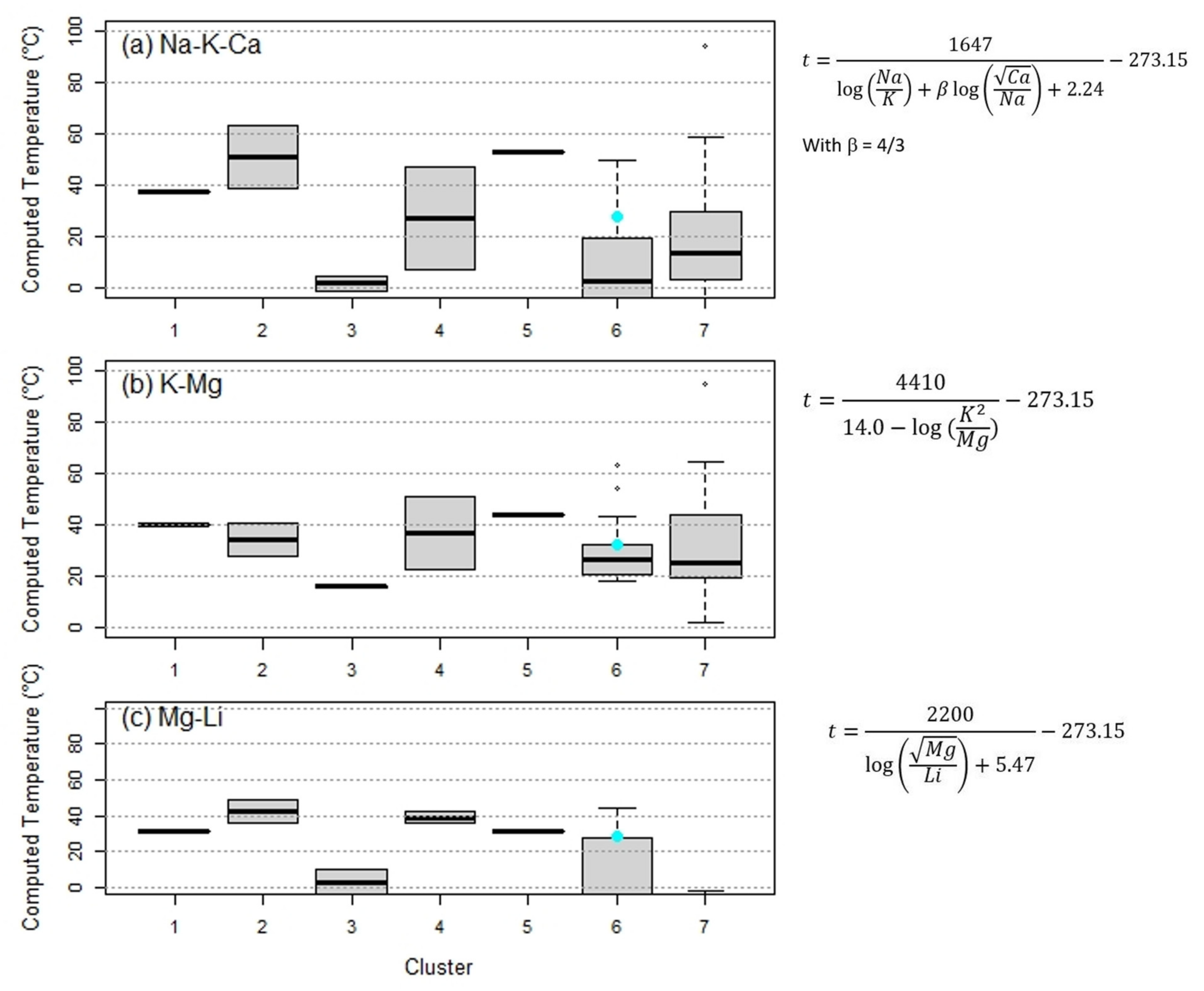
Another widely applied geothermometer is based on the ratio Na/K and its development results from a series of empirical observations combined with experimental and thermodynamics modelling. As such, the Na/K-based geothermometers cannot be directly applied since they are valid only for high temperature conditions (>180 °C) [54,55,56] likely to be above the temperature conditions in the Havelange demo-site case. Furthermore, the computations are based on feldspar stability conditions, which are not the main mineralogical phases in the studied part of the Rhenohercynian fold-and-thrust belt. To extend the field of application of such geothermometer, Fournier and Truesdell [54] includes in the equation the Ca concentration. The range of temperatures covered by their geothermometer range between 4 and 340 °C. The Figure 12a shows the computed temperatures with the Fournier and Truesdell geothermometer [54]. The bulk of values is located below 60 °C with the higher temperatures for samples of clusters 1, 2, and 5. The composition of samples from cluster 3 leads to apparent temperature close to zero. The computed temperatures in cluster 6 are shifted towards low and even negative values, while the superficial water from cluster 7 is promoted to higher and more likely unrealistic values.

The Na-K-Ca geothermometer of Fournier and Truesdell [54] was criticized due to deviation for low temperature and modifications, or new geothermometers were published. Giggenbach [55] proposes the application of a K-Mg geothermometer for low temperatures. The computed temperatures based on the equation of Giggenbach on our dataset (Figure 12b) show, globally, the same trend that the Na-K-Ca geothermometer, but the temperature for samples are less spread and negative values are absent. Finally, Kharaka and Mariner [57] proposed an equation based on the ratio Mg/Li (Figure 12c). Following this model, the computed temperatures for clusters 1, 2, 4, and 5 are between 31 and 49 °C. Some of the samples from cluster 6 drops to negative values and the very low Li-content from superficial waters of cluster 7 lead to only negative values.

The previous three geothermometers predict a reservoir temperature for the Chaudfontaine of 27.6 °C for Na-K-Ca, 32.5 °C for K-Mg, and 28.9 °C for Mg-Li. These values are below the recorded temperature during the sampling site (36 °C), indicating that these geothermometers predicts too low values for the reservoir. A possible interpretation for such uncertainties is the impact of high-Ca and high-Mg concentrations in the studied samples. More specifically, the Ca, Mg contents in clusters 4 and 6 tends to draw downward the values for these groups. Giggenbach [55] evaluate the impact of calcium in the reactions and concluded that the problems of the Na-K-Ca geothermometers result from sensitivity on variations on CO₂-content in the geothermal waters. For the case of the Na-K-Ca geothermometer, one of the assumptions (excess in silica) for the establishment of the equation is probably not met (see the silica geothermometer).

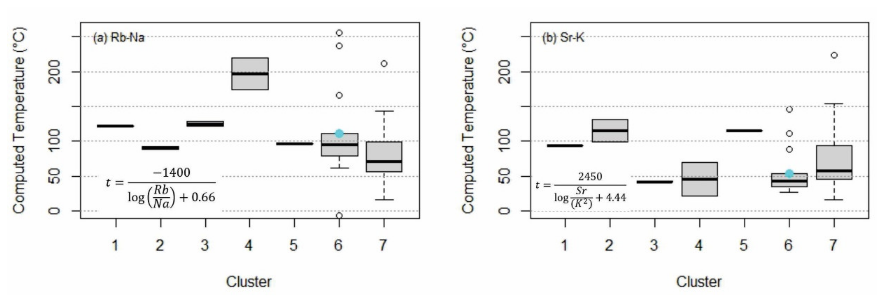
The last geothermometers to be considered here were developed to evaluate the behaviour of, and trace elements from, major hot water reservoirs in granitic terranes [58]. This study covers several domains in Europe and showed that the concentrations in the studied elements are not significantly affected during the flow from the reservoir to the surface for alkaline water conditions (pH > 9–9.5). The water samples collected during the Havelange demo-site campaign show that alkaline conditions are encountered for samples of clusters 4 and 6, while the other clusters gather slightly acidic water. The geothermometer equation for the Rb/Na ratio corresponds to a low temperature aquifer from Bulgaria. If this geothermometer is applied to the Havelange demo-site dataset, it comes out that the computed temperatures are significantly higher than those predicted by the previous geothermometers (Figure 13a). For all clusters, except the last one, all temperatures are largely higher than 50 °C and in the case of cluster 4, temperature estimations even reach values above 200 °C. Similar observations can be conducted for some outliner values of cluster 6. For this geothermometer, the reservoir temperature in Chaudfontaine would be 110.8 °C. Interestingly, these higher temperatures are associated with the clusters of alkaline waters, which are closer to the field of application of this geothermometer. On the other hand, the evaluated temperatures for the superficial waters of cluster 7 are clearly too high.

The Sr/K geothermometer also indicates high values: c. 100 °C for samples from clusters 1, 2, 4, and some outliners of cluster 6. By contrast, temperatures for cluster 3 and 4 show a more reduced values around 50 °C (Figure 13b).

If we compare all computed temperatures with the different geothermometers, it is challenging to identify a clear trend since the temperature ranges are very broad. In a general sense, the temperatures evaluated from the concentrations of major elements (SiO₂, Ca, K, Na, Mg) indicate low temperatures for the geothermal reservoirs. Some of these values are clearly underestimated as indicated by the reservoir temperature that would be inferior to the recorded value at the collecting point (Chaudfontaine). Numerous assumptions can be considered, but a likely feature is the global low concentrations in many of these major elements, with respect to geothermal water. This deficit in major elements was already developed for the silica concentration. The values Lkm (log(K²/Mg)) and Lkc (log(K²/Ca)), as defined by Giggenbach [55], are very low (<0), indicating that the potassium concentration is larger than the square root of Mg and Ca. When reported into a triangle plot of Na, Mg, and K concentration, all points from the current study plot in the Mg corner correspond to immature waters, that is, far from the fully equilibrated waters.

The second category of tested geothermometers are based on the concentration of minor element (Li) or the ratio of a minor elements (Li, Rb, Sr) and a major element (Na, K, Mg). For those cases, the evaluated temperatures are usually higher than for the major element-only methods. The presence of a major element in low concentration associated with a minor element in the geothermometer equations has probably the reverse effect of overestimating the reservoir temperature. The unrealistic temperatures of superficial waters (cluster 7) are clearly the sign of this overestimation. Qualitatively, the real temperatures are probably between the two categories of geothermometer.

6. Discussion

The geothermal exploration must follow a multidisciplinary approach, especially in an unconventional and mainly blind geothermal system. This study case uses the geochemistry of spring water for leading an investigation around the gas exploration well of Havelange, which is here under investigation for a reconversion in a deep geothermal development project. As a result, the common procedure of first conduct exploration at the regional scale followed by a downscaling approach towards sweet spots for the evaluation and development of geothermal cannot be followed, since the borehole was already implemented and drilled in the 80′s without any geothermal objective. It is, therefore, difficult to answer fundamental questions such as: are there significant deep fluid flows? Or if another borehole needs to be drilled to develop a geothermal doublet, where is the best place to intersect the deep fluid flow(s)?

On the other hand, the presence of such deep borehole crosscutting a whole sequence of Devonian metasedimentary formations is relatively unique. It allows us to investigate the geothermal potential of an unconventional reservoir, which consists of fracture tight metamorphic units in a fossil fold-and-thrust belt and in a zone where the presence of post-Variscan extensional fractures is absent or very-limited. The Havelange borehole is, therefore, a good candidate for exploring and evaluating the development of a geothermal system in such unconventional conditions. The success of such a project would unlock new possibilities for the development of the geothermal industry in regions where conventional targets are not available. These regions include many places in the Rhenish Massif in Germany, Northern Luxembourg, a large portion of southern Belgium, and the buried basement under the London–Paris basin.

In this paper, the various subsurface fluid flows around the Havelange deep borehole were analysed by studying the groundwater geochemistry composition from mainly springs and a few other infrastructures (wells, a drainage gallery). The dataset includes physicochemical parameters recorded in a laboratory and in the field of 50 sites in the near field (NF) (< 5 km from Havelange borehole) and the far field (FF). The Lower Devonian rocks from the FF represent the ground surface analogue formations to those observed in the deep part of the Havelange borehole. One of the samples was also acquired from a water catchment in the city of Chaudfontaine and is used here as a hydrothermal reference.

The analysis results treatment includes conventional data representations of aquifer composition in hydrogeology such as the Piper and Stiff diagrams along with a multivariate approach to define compositional affinities/dissimilarities between the samples. Several geothermometers such as chalcedony, quartz, lithium, Na-K-Ca, K-Mg, Mg-Li, Rb-Na, and Sr-K were also used to evaluate reservoirs temperatures.

The results show a broad variability of the compositions and various clusters, or groups can be identified. The number of clusters is, however, dependant of the applied method and of the analyst choice. For this study, seven clusters were identified with the hierarchical clustering method; the heat map representation indicates three main horizons of compositions. Even if the data-treatment methods provide different numbers of clusters, they globally tend to similar groupings with marginal variation for intermediate composition.

The largest group from the hierarchical clustering corresponds to superficial water, slightly acidic and with frequent high NO₃ levels more likely related to agricultural activities. This group is also characterised by a low electrical conductivity, a low TDS level and, hence, a narrow Stiff polygon. A strong relationship is observed between these superficial water discharges and the presence of detrital formation of Famennian age in surface geology. The known barrier or cap rock behaviour of the Famennian formations, especially the lower Famennian shale, is here confirmed.

At the other end of the composition spectrum, a few springs in the FF show acidic water and a high mineral charge. These springs are known in the region as ‘pouhons’ or carbogaseous springs and they are associated with detrital metasedimentary rock of either the Lower Devonian or Lower Palaeozoic age. The iron and manganese contents are very high and indicators of thermal water such as Li, Sr, and Rb are also observed in high concentration. The NO₃ levels in this group is very low.

A third important group corresponds to slightly alkaline water with a significant mineral charge and high levels of the Li, Sr, and Rb indicators. The mineral composition is, however, different from the previous carbogaseous group. Samples from this third group are acquired in the NF and especially in an area located about 4 km to the East of the Havelange borehole in the villages of Moressée and Heure. Such composition of water in the region was not yet coined and provide new valuable information. In addition, during the field campaign several springs in the NF shown the presence of gas. Besides these occurrences in the NF, the reference hydrothermal water from Chaudfontaine also belongs to this group. In other words, water samples from this group in the Havelange borehole NF have, therefore, affinities with the hydrothermal water of Chaudfontaine. The water composition of this group is interpreted as water discharges from a deep, partly confined, aquifer developed in either Givetian or Frasnian limestone formations. The discharge of this aquifer at ground surface and, thus, through the confining beds of Famennian formations is probably the result from the presence of a draining fracture zone.

Besides these three large groups of composition, other springs are characterized by intermediate composition that reflects transitions; either a local specificity (e.g., mineral deposits) or the mixing of water from different composition groups.

At this stage of the exploration, it is delicate to evaluate the significance of the fluid flow between the aquifer located in the Givetian and Frasnian limestones and those located deeper in the detrital Lower and Mid-Devonian formations observed in the deep part of the Havelange borehole. As a first approach and following the spring water composition observed in similar rocks in the FF, it is likely that the water in the deepest part of the Havelange borehole is acidic with a significant mineral charge, include significant concentration in Fe, Mn. In a hypothesis of a water flow upward from the deep subsurface, it will reach the limestone beds and their associated aquifer, and a series of reactions will take place, such as a dissolution of the limestone and the production of dissolved CO₂. The presence of gas in several springs from the NF is a probable indicator of such reactions.

The application of geothermometers in a metasedimentary context of a fold-and-thrust belt indicates various results and shows different limits. In fact, the use of one type of geothermometer rather than another is based on a supposed reservoir temperature and on the phase equilibrium. In this study, we considered that the reservoir is around 100 °C. Of the nine geothermometers used, only two seems to show convincing results (quartz and lithium). Indeed, if the Chaudfontaine site is taken as a reference (temperature of 36 °C at the surface), the results obtained with the use of chalcedony (29.9 °C), Na-K-Ca (27.6 °C), K-Mg (32.5 °C), and Mg-Li (28.9 °C) geothermometers do not seem realistic (not to mention the negative values in some clusters). The higher concentration of Ca and Mg in some clusters may explain the calculated low temperature and the presence of CO₂ and silica deficiency may interfere with the use of the Na-K-Ca geothermometer. Geothermometers based on major and trace elements indicate very high temperatures (Chaudfontaine temperature 110.8 °C (Rb-Na)). Moreover, the superficial water reservoirs would be at more than 50 °C due to the higher concentration of major elements than trace elements.

Regarding geothermometers, which seems to indicate more consistent results, quartz can be used for reservoirs above 180 °C and research in granite massifs has shown that it remains applicable below 90 °C in this environment. It would be necessary to conduct a study to verify the applicability of this method to a geological context like the Havelange. If the quartz-based calculations are applied to Chaudfontaine, the reservoir temperature calculated in this paper is about 62 °C instead of 50 °C found by Graulich in the 1980s.

The geothermometer based on the lithium concentration also shows values that seem consistent although overestimated. However, the application of this tool should only be done when the clusters contain a significant content of Li, otherwise negative temperatures are calculated.

In view of these diverging results, the questions would be: is it possible to use these geothermometers in the geological context of the Havelange, namely meta-sediments in fold-and-thrust belt? Are these variations due to dilution effects or to the unavailability of the necessary mineral phases in the water?

7. Conclusions

In this study, the geochemical composition analysis of spring water is applied as a surface tool for deep geothermal potential exploration. It aims to detect the geochemical indications of the impact of ascending deep-water flow on the composition of spring water samples. This approach is of particular interest in blind geothermal systems where there are no clear surface manifestations of the presence of a deep geothermal system. The technique is here applied to water samples collected in the near and far field around the Havelange borehole. This site is the selected H2020 MEET project demo-site for the evaluation of the geothermal potential of the unconventional reservoirs in the Variscan metasedimentary system, unaffected later by an extensional deformation phase.

The results show that the water samples can be separated into different clusters of compositions revealing different water evolutions. The number of clusters is dependent on the statistical method applied for the data treatment. Using the hierarchical clustering, seven clusters can be evaluated and related to different combination of concentrations/values of elements or parameters such as Li, Rb, Sr, pH, and EC. The application of the heat map technique demonstrates the presence of at least three types of water. The first group consisting of water sources locally known under the name of “Pouhon”, is characterized by an acidic pH, a high EC, and TDS and by the frequent presence of anomalies in Fe, Mn, Ni, Be, Mg, and Li. The second group is represented primarily by carbonate water compositions with neutral to basic pH as well as high EC and TDS. Bromide, Mo, U, V, Se, Sb, Li, Rb, Sr, and Cu anomalies are frequently observed in this category. The Chaudfontaine reference hydrothermal site and the samples located in Eastern neighbourhood (near the village of Moressée) belong to this second type. Waters from this category constitute the targets for future geothermal studies. In fact, the water samples around the village of Moressée show higher concentrations of Li, Sr, and Rb than in Chaudfontaine. The third and last group contains superficial waters with a low conductivity and TDS. They exhibit a high concentration of NO₃ and low concentrations of Li, Rb, Ca, Na, K, Mo, and HCO₃. These superficial waters are frequently associated with the outcropping zone of lower Famennian formations that represent an aquiclude and act as a cap rock for the deep-water reservoir. Future investigations will need to focus on other categories of analyses such as the isotopic and gas content.

In addition, this paper shows that the use of geothermometers in the Havelange context, and probably more broadly in metasedimentary fold-and-thrust belt domains, need to be considerate with caution. In fact, the low temperature presupposed (around 100 °C) and the lack of knowledge on the phase balance in the reservoir suggest that the method can hardly directly be applied with commonly used geothermometers (chalcedony, quartz, Li, Na-K-Ca, K-Mg, and Mg-Li). A hydrogeochemical model of the reservoir would possibly provide indication of the water composition evolution in our system and to develop geothermometers usable in this geological context.

To conclude, the indication of deep fluid flow in the region of the Havelange borehole is a significant information, but at this stage it is difficult to evaluate if such phenomenon is restricted to a small zone around the study site and if it can be extrapolated to numerous zones of occurrence of Variscan meta-sedimentary formations. If this second option could be verified, it would open new opportunities for the development of deep geothermal projects in numerous regions of North-West Europe, such as the Rheinische Schiefergebirge in Germany, the Oesling in the Great Duchy of Luxembourg, the Ardenne in Belgium to even Devon and Cornwall in SW-England.