Distributed Cooperative Avoidance Control for Multi-Unmanned Aerial Vehicles


Temasek Lab., National University of Singapore, Singapore 117411, Singapore
*
Author to whom correspondence should be addressed.
Actuators 2019, 8(1), 1; https://doi.org/10.3390/act8010001
Submission received: 16 October 2018
/
Revised: 21 November 2018
/
Accepted: 19 December 2018
/
Published: 21 December 2018
Abstract
:It is well-known that collision-free control is a crucial issue in the path planning of unmanned aerial vehicles (UAVs). In this paper, we explore the collision avoidance scheme in a multi-UAV system. The research is based on the concept of multi-UAV cooperation combined with information fusion. Utilizing the fused information, the velocity obstacle method is adopted to design a decentralized collision avoidance algorithm. Four case studies are presented for the demonstration of the effectiveness of the proposed method. The first two case studies are to verify if UAVs can avoid a static circular or polygonal shape obstacle. The third case is to verify if a UAV can handle a temporary communication failure. The fourth case is to verify if UAVs can avoid other moving UAVs and static obstacles. Finally, hardware-in-the-loop test is given to further illustrate the effectiveness of the proposed method.
1. Introduction
Currently, the cooperative control of a multiple unmanned aerial vehicle (UAV) system is attracting growing interest. This is motivated by the constantly growing number of civil and commercial UAV applications [1]. One of the core problems in multi-UAV systems is motion planning, where each UAV navigates a path to the target by sharing each other’s information. This should result in a collision-free path derived from UAV motion control. This has driven the development of various UAV collision avoidance algorithms.
UAV collision avoidance necessitates a way to predict UAV motion. There are different methods to predict UAV motion and the future positions of the UAV. Early collision avoidance strategies focus on the static obstacles [2,3], using decision trees to avoid various troublesome situations [4], and using path planning to avoid the obstacles [5]. As moving obstacles are more often found in a real environment, many techniques have been proposed for dealing with this situation. For example, in [6], the authors developed a vision-based collision avoidance method by using minimum effort guidance. In [7], the authors presented a reactive avoidance method by using nonlinear differential geometric guidance; in [8,9], the authors developed a local path planning method for UAV navigation; in [10], the authors presented a collision avoidance algorithm by using dynamic programming; in [11], the authors proposed a collision avoidance algorithm based on potential fields; in [12,13,14,15,16,17], the authors presented the velocity obstacle method for deconflicting the UAV paths. Among these methods, the velocity obstacle has been the most actively studied in multi-UAV control over the past ten years. These include methods from avoidance maneuver based on conflict geometry [12]; optimal reciprocal collision avoidance [13]; reciprocal collision avoidance using on-board decentralized sensing without communication [16]; the recursive probabilistic velocity obstacles algorithm [14]; the hybrid reciprocal velocity obstacle algorithm [15]; and the artificial bee colony optimized reciprocal velocity obstacle algorithm [17]. However, each of these methods suffer from at least one of the following limitations:
- Each UAV acts independently without coordination with other UAVs, giving rise to deadlock;
- Each UAV acts with full coordination with all other UAVs, requiring excessive communications;
- A heavy computational load is required.
The aim of this paper was to develop an efficient avoidance method that does not suffer from any of these limitations. The basic idea is to use the cooperative control concept. First, multi-UAV communication is proposed to exchange UAV information. Second, a fusion algorithm is proposed for forming a heartbeat message which provides the cooperative information of UAV-to-UAV. Third, with the heartbeat message, the algorithm the UAVis designed to select the velocity command to avoid only those UAVs or obstacles that are within a certain range around the UAV. This control is decentralized, and each UAV independently makes its own decision. Finally, simulation and hardware-in-the-loop tests were conducted to illustrate the effectiveness of the proposed method. The contribution of this paper is twofold: designing the information fusion technology to obtain other UAV heartbeats in a weak communication network; and developing a velocity obstacle algorithm to handle polygonal obstacles.
A short version of this paper was presented at ASCC 2017 [18]. The work of [18] has been expanded to include four new parts: (i) we add the related work in Section 2; (ii) we extend the algorithm to 3D space; (iii) we give the algorithm to handle polygonal obstacles in detail; (iv) we modify the algorithm (see Section 3.4) and test more examples, especially in the hardware-in- the-loop simulation.
2. Related Work
Autonomous collision avoidance has been an active research area in unmanned aerial vehicle control. These include the path planning method [9], the conflict resolution method [19], the potential function method [11], and the velocity obstacle method [12]. Because it is less computationally complex, the velocity obstacle method is attractive in giving a fast solution in a dynamic environment. We shall briefly review a few of the most closely related works in the velocity obstacle method.
The original concept of the velocity obstacle is introduced in [20]. The authors describe the collision cone concept, where the collision cone is a set of vehicle velocities that will cause a collision with the obstacle if the obstacle’s velocity is constant. However, this work only discusses the case where two UAVs avoid collision with each other, and only provides the concept of avoiding polygonal obstacles without implementation details. In this work, no simulation is given to verify the proposed method. In [12], the authors define another velocity obstacle cone in a velocity space by moving the collision cone by the obstacle’s velocity. In [21], the authors introduce a non-cooperative concept for avoiding collision by assuming that the distance, direction, and range of speed of the obstacle are known. In this work, the feasible velocity set is obtained by checking speeds in the obstacle speed range. However, the computational cost is very high, and it is not suitable for MUAVs. In [14], the authors use the probability concept to represent collision. If the feasible velocity leads to a collision with an obstacle, it is denoted as 1; otherwise, it is 0. Using this approach, the proposed method can calculate the collision chance for MUAVs. This requires a perfect communication network. However, the obstacle is assumed to be circle-shaped, and only two vehicles were tested in their simulation. In [22], the authors introduce “the passing on the right rule” to the velocity obstacle method in order to provide a safety rule. In [23], the authors present an extension of [12,22]. In this work, the avoidance rules are designed based on conflict geometry. However, the authors assume that a full communication oriented system is necessary without failure.
It is observed in [24] that the traditional velocity obstacle method has an oscillation behavior. To overcome this issue, the authors in [13,24] present a reciprocal velocity obstacle (RVO) method. In this work, the authors suggest to move the collision cone by , where is the vehicle velocity and is the obstacle velocity, instead of moving by as in the original velocity obstacle approach [12]. In [16], the authors use the RVO method based on an onboard sensor without communications. Furthermore, in [17], the authors propose the use of a genetic algorithm in RVO to find the optimal velocity set. However, it is still observed that undesirable oscillation exists in the RVO approach when more than two vehicles are tested. In [15], the authors propose a hybrid reciprocal velocity obstacle method by using an asymmetrical collision cone. However, their results showed that the collision chances increased with an increasing number of vehicles.
So far, there is a limited body of literature considering sensor constraints. In [25], the authors propose a reciprocal collision avoidance algorithm, where the robots use their camera with a limited field of view to detect the environment. However, this result is not feasible for MUAVs, since the limited sensor has a large dead zone and cannot react rapidly in a multi-UAV system where UAVs can approach from the sides undetected.
The limitations of each method are summarized in Table 1. For each method, we check if it considers the requirements listed in the columns. “Suitability for MUAVs” indicates if the method is suitable for a MUAV system. “Robust to communication failure” indicates if it requires communication to be perfect. “Cooperation” indicates if it can share information with other UAVs to work together. “Low computational cost” indicates if the solution can work with minimal computational resources. “Polygonal obstacle” indicates if the solution can be applied to handle polygonal obstacles.
For our MUAV system, the collision avoidance method should be scalable, and can handle any number of UAVs as long as the traffic density does not become infinite. Obviously, this requires a distributed control form. Additionally, since a UAV has to face various obstacle shapes, it is important to consider a shape that can represent general irregular shapes for obstacles. From the table, it is observed that every method has some limitations and cannot satisfy all requirements. This paper proposes a distributed cooperative control method that addresses all these limitations.
3. Problem Statement and Solution
The overall goal of the multi-UAV system is to reach all the targets without collision in the working area. Let us consider M targets in the entire zone and N UAVs that need to be assigned to these targets. Define a set of UAVs as , and targets as . Our problem is to design a collision avoidance algorithm which drives a UAV to its assigned target safely. The solution to this problem is to be in a decentralized form. In this framework, each UAV makes its own decisions based on its own onboard GPS data and communicated information from other UAVs.
3.1. Communication
In this paper, the multi-UAV system uses the User Datagram Protocol (UDP) [26] for the wireless communication. With UDP, UAVs in the network can broadcast their messages regularly at the frequency , and it is not necessary to wait for acknowledgment from other UAVs. The UAVs are connected but not necessarily fully connected. The UAV nodes are organized in a mesh topology. The reasons for the use of the UDP mode are that we want the latest message from other UAVs regularly and we want to save energy by reducing transmissions.
3.2. Cooperation through Shared Heartbeats
The cooperation task described in this section is the sharing of information among UAVs through one-hop heartbeats. A heartbeat message is formed by fusing together received heartbeats and a UAV’s own onboard information. The information exchanged heartbeat (HB) is given in Table 2.
In an N UAV system, if the communication is working well, each message has information from N UAVs. Each UAV receives HB messages from other UAVs. This implies that it has N HB messages including itself. In our system, all messages are placed into the MessageBox. The total messages at each time interval in the MessageBox has messages. Obviously, there exists redundant information in the MessageBox. The next question is how to fuse to the messages to reduce the information size, thereby generating the HB of the UAV. Each message is attached with a GPS time stamp. Thus, we know the latest message if we compare all GPS time among the messages in the MessageBox. Here, we use a search algorithm (see Algorithm 1) to find the latest message.
| Algorithm 1: Search algorithm |
| Input: UAV ID, HB from other UAVs |
| Input: HB of UAV |
| for m = 1 to length of total UAVs do |
| tmp = 0 |
| for h = 1 to length of total UAVs do |
| if GPS T of HB[h*total_UAV_Num+m] |
| >= tmp then |
| tmp = GPS T of HB[h*total_UAV_Num + m] |
| store HB[h*total_UAV_Num + m] information |
| end if |
| end for h loop |
| end for m loop |
Let us consider a UAV . At each time interval, the UAV receives HB messages from other UAVs, which are placed into the MessageBox of UAV according to the order number of the UAV Identification (ID). Then, we check the j-th UAV information () from all HB messages in the MessageBox. This starts from the 1st UAV message and we check if it has the latest GPS time for the jth UAV message. If so, it will extract the jth UAV information from the 1st UAV message and put it to the HB message of UAV . However, if the GPS time of the jth UAV information in the 1st UAV message is not the latest, it will check the next UAV message in the MessageBox. This process continues until it finds the latest message of the jth UAV from UAV . Repeating this process, we can find the latest UAV information of all UAVs from the UAV HB messages received and from the HB message of UAV at this time interval.
The HB message of UAV thus obtained will be broadcasted at the next time interval. Over some period of time, the HB messages will converge to some stable form for the given number of UAVs if the communication network is connected. This process is the fusion of information. In this way, we can guarantee that the ith HB formed will consist of the latest UAV information received. The information fusion is illustrated in Figure 1. After the fusion, the HB at each UAV only has the latest information of N UAVs.
We can use the following protocol to represent information fusion for the i-th UAV which contains the h-th UAV HB:
where represents the HB of the jth UAV received by the ith UAV, and is the weighting of the information fusion, that is:
Thus, we use to represent all possible HBs received from other UAVs:
where , and
Note that for each row in the matrix , the weighting set of has only one element which is equal to 1 due to the searching result, and other elements are zero. This implies that
Therefore, we conclude the following consensus theorem.
Theorem 1.
Assuming that the communication is a mesh network (partial or fully mesh network), the HB information of the multi-UAV system with protocol (1) achieves consensus as . By Theorem 1, the cooperation of the multi-UAV system can be implemented through the proposed protocol.
Remark 1.
The proposed cooperation mechanism can handle the weakly connected communication network. For example, Figure 2 shows three types of weakly connected network graphs. By exchanging and information fusion, the proposed method is robust against weak communication in the network.
3.3. Cooperative Collision Avoidance
The collision avoidance algorithm requires that all UAVs broadcast their position and velocity regularly at f Hz. This is done cooperatively through shared HBs, as shown in Figure 3. Each UAV takes the position and velocity of all UAVs within communication range and computes a flight speed and direction command in the horizontal plane. This command is computed and sent to the UAV flight control board, which sends actuator commands to the UAV. The whole process is shown in Figure 4.
The algorithm works not only in the horizontal plane, but also in the vertical direction. For the own UAV and another UAV j, the own UAV has to check if
- Horizontal distance between both UAVs ≤ rang1; and
- Vertical difference between both UAVs ≤ rang2.
If both conditions are satisfied simultaneously, the own UAV enters the collision avoidance mode; otherwise, the own UAV is free and can use any control command. In this paper, climb speed commands are decoupled from the collision avoidance commands in the horizontal direction.
If both conditions are not satisfied, the collision avoidance rules for the vertical direction are:
- Keep the vertical speed (i.e., climbing or descending) command;
- UAV does collision avoidance in the horizontal direction at the same time.
3.3.1. Collision Avoidance between Two Moving Vehicles
The own vehicle A considered is a point object, moving at a speed . The vehicle A first checks if the vehicles around it are within its range (denoted as maximum range), as shown in Figure 5. The detection of collision avoidance only considers those vehicles which are within the lown vehicle’s maximum range. Furthermore, the vehicle A also detects the vertical direction and does the height difference check from neighbouring UAVs. If the height difference between both UAVs is less than the defined value, collision avoidance will handle this case; otherwise, collision avoidance will not consider this case. The algorithm is based on the velocity obstacle (VO) method [12], which uses the concept of the collision cone along the horizontal plane.
Before using the VO method, vehicle A checks if the vehicles around it are within the own vehicle’s maximum range and height difference. If yes, for those vehicles within the defined height difference, it will separate both vehicles by moving the own vehicle until they are at a safe distance.
Consider the own vehicle A, and the circle B which is constructed by the obstacle vehicle B with a radius , where is a safe distance between vehicle A and obstacle B. Figure 6 shows the concept of velocity obstacles. For a given vehicle B moving at velocity , the in the velocity space of the vehicle A is a cone which is the infeasible velocity command candidate set. It is produced by finding two tangent lines (line 1 and line 2) to the circle B from the center of the vehicle A and moving the collision cone by .
A velocity command candidate in this cone set is infeasible because it would lead to a collision with the other vehicle when both vehicles hold their velocities constant over time.
The collision cone is useful for vehicle A to select its avoidance velocity set to avoid a future collision within a given time interval. The key selection criteria for this set are to choose those velocities which never fall into the collision cone. Define a normal vector to line 1 (line 2). An alternative expression of the selection criteria is that the vector should be chosen so as to be outside the collision cone. Both selection rules will avoid the obstacles.
Motion safety is also important for the velocity obstacle method. Assume that the maximum velocity of UAVs is , while the maximum braking deceleration is b. We have the following theorem.
Theorem 2.
If a UAV is in a safe distance from one obstacle initially, then the UAV is able to brake to a complete stop at all times without colliding with the obstacle.
Furthermore, each selected velocity is subject to the actual velocity constraints. This avoidance velocity set is called the reachable avoidance velocity (RAV).
For vehicle A, a velocity command candidate avoiding vehicle B can be obtained by selecting any velocity in the RAV set. Moreover, this velocity command can be classified into the three regions according to the collision cone and the positions of both vehicles A and B. This is because the relative velocity of vehicle A outside the collision cone is guaranteed to be free from collision if vehicle B keeps its current velocity constant. Figure 7 shows that a velocity command candidate can fall into one of the three regions: region is between and , region is between and , and region is below the line , where the lines are the tangent lines of the collision cone, while the line is perpendicular to the center line of the collision cone. Since the regions are outside the collision cone, they are safe. The velocity command should be selected from these three safe regions.
Consider actual traffic conditions and rules. We suggest alternative velocity options so that the vehicles will not get stuck in traffic. Take, for example, incorporating the rule of passing on the right [22]. This is based on the rules of the sea, the International Regulations for Preventing Collisions at Sea (COLREGS), as shown in Figure 8. These are similar to the Federal Aviation Administration (FAA) rules of the air. Applying this rule to the RAV set will avoid deadlock. This can be observed when two vehicles approaching head-on try to avoid each other but instead steer to the same side. They would then be unable to pass each other. The rule can be adopted especially with the velocity obstacle concept, as we can restrict the velocity command options to make the vehicle pass on the correct side of the other vehicle. According to the rules of COLREGS, velocity sets and are selected as the avoidance velocities. Thus, they are reachable avoidance velocities and are safe for driving vehicle A.
3.3.2. Collision Avoidance between a Vehicle and a Static Circular Obstacle
For static obstacles, we have to modify the collision cone when selecting an avoidance velocity set. This is because a static obstacle is not more dangerous than moving obstacles. Considering static circular obstacles, the associated velocity obstacle is as shown in Figure 9. In this velocity obstacle, a user-defined time is introduced such that the feasible region is enlarged. Compared to the velocity obstacle due to moving vehicles, this is smaller in that velocities towards the obstacle are permitted if they take more than time to make contact with the obstacle. Thus, the RAV incorporated with COLREGS should avoid the modified collision cone for dealing with static circular obstacles.
3.3.3. Collision Avoidance between a Vehicle and a Static Polygon
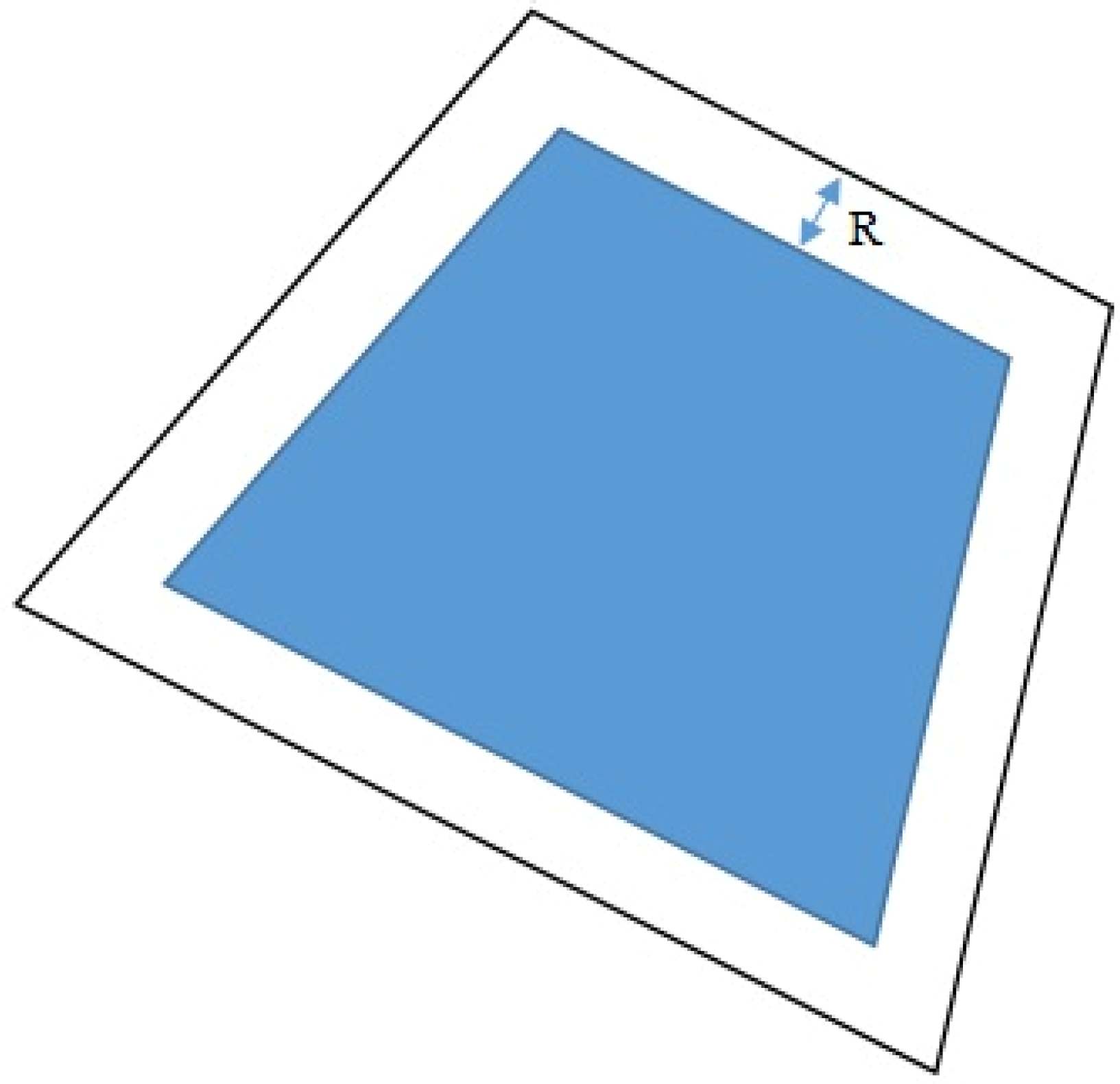
In addition to circular obstacles, polygonal obstacles are also considered. Unlike circular obstacles, polygonal obstacles have complex shapes. These polygonal obstacles fall into two general categories: convex and non-convex. In general, a non-convex polygon can be considered as consisting of several convex polygons, as shown in Figure 10, where the non-convex polygon is partitioned into three portions: convex polygons , and . It is necessary to design the algorithm to avoid each of the convex polygons. Thus, we concentrate on convex polygons in this paper and find the avoidance approach. To include a safety buffer, we first need to expand the polygon obstacle to draw a region of safe constant width around it, as shown in Figure 11. Throughout this paper, we assume that the polygon was expanded with a safe constant width R.
In order to find a feasible region from a convex polygon, we have to calculate the centroid of a polygon. For a closed polygon consisting of n vertices , its centroid is denoted as . Their values are given by
where A is the polygon’s area, which is described by
Thus, by connecting a vehicle point and the centroid of a polygon, a ray is formed as shown in Figure 12. This ray goes through the segment splitting the polygon space in two parts, called the half-space as shown in Figure 12. We are concerned with the angle between this line and the vertex of the polygon. For each half-space, we can obtain the angle between the line and vertex of the polygon. For example, as shown in Figure 12, we have the angles 1–2 for the right side of the line, while we have angles 3–4 for the left side of the line. From the collected angles of each half-space, we can obtain a maximum angle and thus a collision cone is formed for the polygon. A velocity command avoiding the polygon can be selected from outside the collision cone.
Remark 2.
Some papers deal with polygonal obstacles. For example, the work in [27] uses a path planning approach to handle polygonal obstacles. In this paper, we want to improve the VO method such that it can be applied to many situations, including polygonal obstacles. This is convenient for application purposes. In addition, it should also be noted that it is difficult to use the approach proposed in [27] to deal with moving obstacles, since the computed trajectories depend on the pre-defined static objects. In comparison to the work of [27], the VO method is more suitable for dealing with moving obstacles.
3.4. Collision Avoidance Algorithm
The safe set of velocity commands is represented by all points within the maximum velocity circle and outside all the velocity obstacles. The velocity command to choose would then be the one that has the least deviation from the desired velocity command which points directly toward the waypoint to head for. The detailed steps of the algorithm are as follows:
Step 1. Check all the other vehicles within the 3D range (i.e., maximum range and height difference).
Step 2. For those vehicles within the defined height differences, the primary vehicle does a separation movement in the horizontal plane until reaching a safe distance , where is the radius of the primary vehicle, and is the radius of another vehicle around the primary vehicle.
Step 3. Find the admissible regions given all the other vehicles within the 3D range and safe distance (user-defined).
Step 4. Find the admissible regions given all the static circular obstacles and polygonal obstacles within a certain range (user-defined).
Step 5. Find the cost for each admissible speed–direction option.
Step 6. Find the lowest cost option and apply this velocity to the flight control board of the primary UAV.
Step 7. Repeat the steps above.
Remark 3.
The safe distance of the proposed collision avoidance is required to be 3, where is the maximum speed of the UAV. This implies that if both UAVs are disconnected for two seconds, they still have at least 2 distance under this extreme communications loss situation. This implies that the proposed collision avoidance algorithm is robust against communication failures of up to two seconds of disconnection.
Remark 4.
The primary UAV in the proposed collision avoidance scheme only checks with those UAVs which are within a certain range around the primary UAV and chooses the velocity command from the lowest-cost option. Thus, the proposed collision avoidance algorithm is locally optimal. It will take less computational load than algorithms which use full information from all connections with other UAVs to make the collision avoidance decision. Utilizing full information would incur a heavy computational load, is not practical in real-time UAV control, and is not scalable when increasing numbers of UAVs are involved. In addition, some papers use optimization algorithms to find feasible trajectories to avoid obstacles. In general, these kinds of approaches can take a longer time to search for an optimal solution. For example, the work in [9] uses a non-linear program (NLP) and a mixed integer linear program (MILP) to find trajectories while maintaining the safe separation between UAVs. Unfortunately, the average solution times of the MILP and NLP were 4.32 s and 46.53 s, respectively, as reported by [9]. This is unacceptable for real-time control. In our C program, the solution of the proposed velocity obstacle method took approximately 10 ms.
Remark 5.
The present algorithm also differs from those algorithms which only use information obtained from the on-board sensors and give a limited solution. Onboard sensors are usually unable to provide all-around situational awareness as well as the velocities of other UAVs. This may cause a deadlock problem. In our solution, the weakly connected network is used to exchange HBs from other UAVs, and thus the avoidance can find a feasible path from around UAVs, thereby reducing the possibility of a deadlock.
4. Simulation Study
The purpose of this section is to illustrate the usefulness of the proposed multi-UAV collision avoidance method. Each UAV is regarded as a point mass in a three-dimensional space. The stationary obstacles are depicted as circles. In the simulation, we use C to implement the logic and algorithms and MATLAB as a tool to plot the results.
Case 1: Avoiding a Stationary Circular Obstacle. Consider a scenario where we have ten UAVs and ten targets of two types: the static type, labeled as 0, 1, 2, 3, 7, 9; and the patrol type, labeled as 4, 5, 6, 8. Every UAV will be assigned to a target and will fly to that target, which may be of static or patrol type. Table 3 shows the target waypoints, and the obstacle is a circle with a radius of 30 m. During the flight, they may encounter static obstacles (as shown by the circles in the following figure) or other UAVs. The cooperative collision avoidance algorithm will cause the UAVs to avoid the static obstacle which is located in the center of the working zone. Each UAV communicates with other UAVs using UDP through a regular broadcast of messages every 1 s.
Figure 13 shows the multi-UAV flight paths in the simulation. It was observed that both UAVs effectively avoided the obstacle located in the center of the working area when flying to their respective targets. The results show that the UAV assigned to target 6 was successful in avoiding the obstacle when it flew to it. This was also observed for the UAV assigned to target 0. Figure 14 shows the profile of the horizontal distance between the ith UAV and the jth UAV (). It was observed that the minimum separation distance along the horizontal direction was about 30 m, and no collision occurred. This simulation verifies that the proposed UAV collision avoidance algorithm was effective in avoiding a static circular obstacle.
It was observed that the two vehicles could move along the obstacle to reach their respective targets. This is because the selected velocity always follows the direction of the tangent line of the velocity cone. This ensures smooth turning to avoid collision.
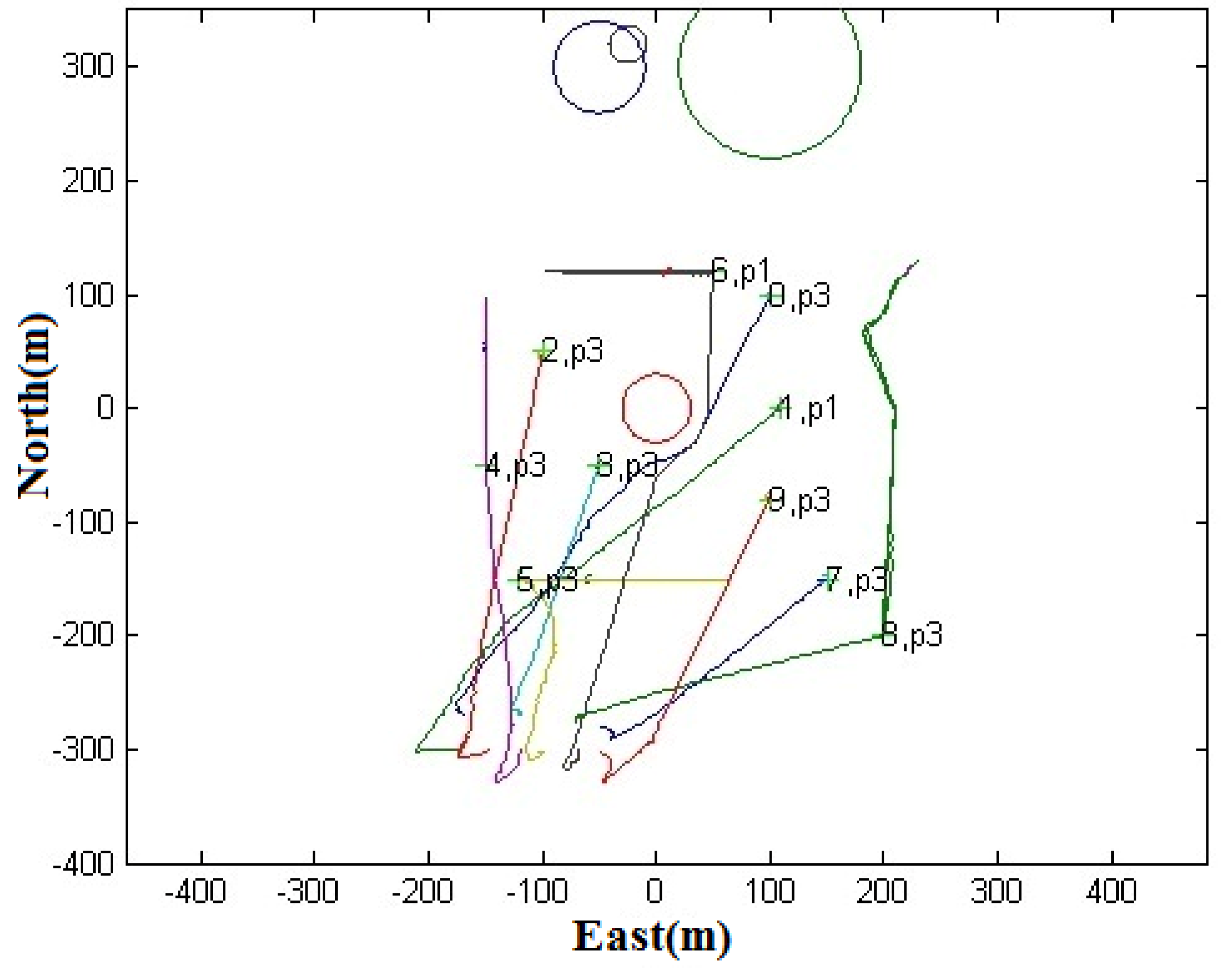
Case 2: Avoiding Polygonal Obstacle. Consider a scenario where we have ten UAVs and ten targets of two types: the static type, labeled as 0, 1, 2, 3, 7, 9; and the patrol type, labeled as 4, 5, 6, 8. Table 4 shows the target waypoints. Every UAV is assigned to a target and flies to that target, which may be of either static- or patrol-type. During the flight, they encounter a polygonal obstacle. The cooperative collision avoidance algorithm will effectively cause the UAVs to avoid the polygonal obstacle, which is located inside the working zone.
Figure 15 shows the multi-UAV flight paths in the simulation. It is observed that four UAVs (UAVs 6, 7, 8, and 9) effectively avoided the rectangular obstacle when flying to their respective targets. This simulation verifies that the proposed UAV collision avoidance algorithm was effective in avoiding a polygonal obstacle.
From the simulation, it was observed that the algorithm was capable of computing the minimum angle to move along in order to avoid collision, as explained in Section 3.4. It should also be noted that vehicle 6 selected the shortest route to its target. This shows that the vertex of the polygonal shape selected as an avoidance direction also depends on whether that vertex is closest to the desired velocity vector. From Table 1, we see that existing results do not consider polygonal obstacles except for [20], which only provides the concept without implementation details.
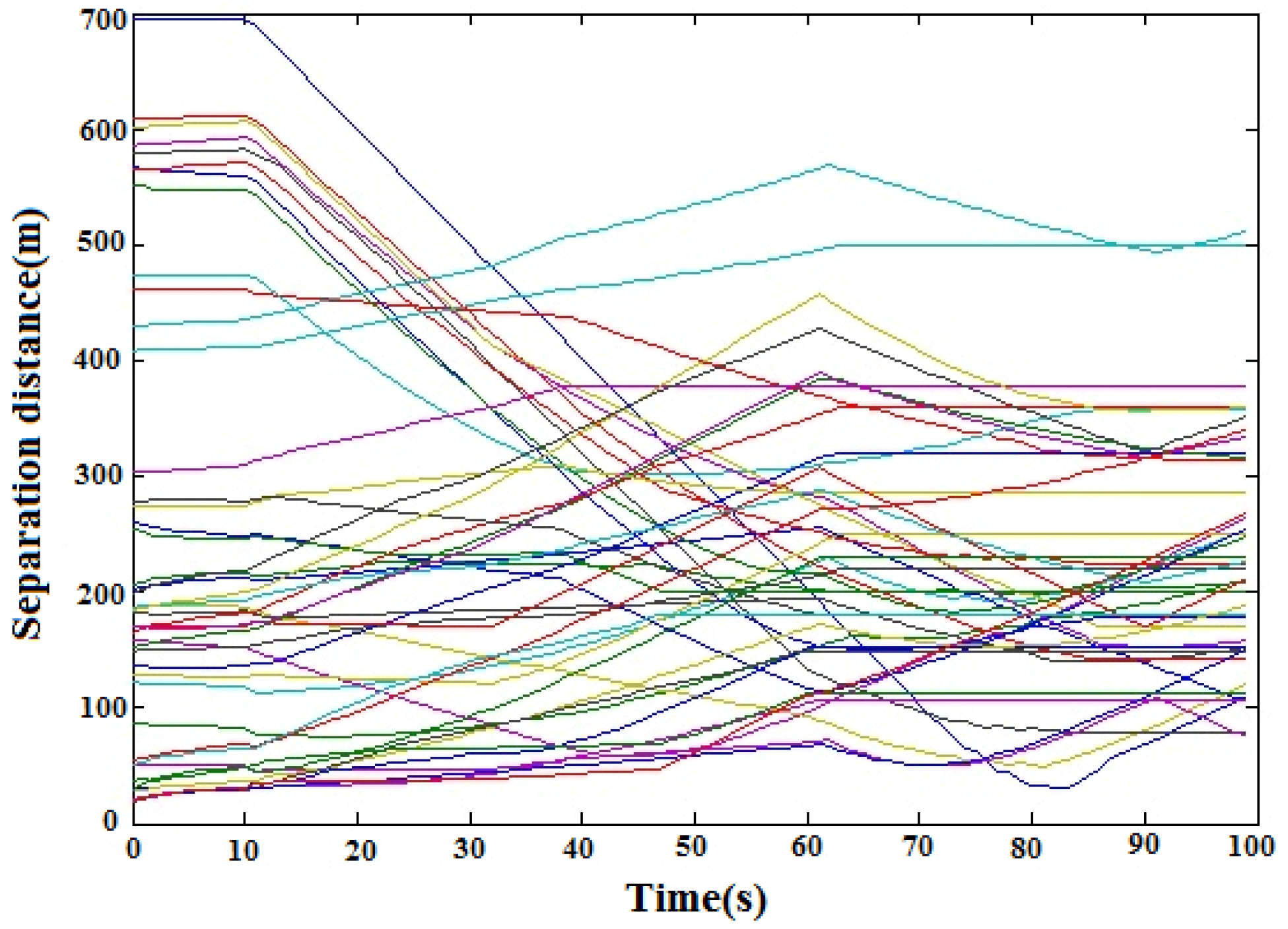
Case 3: Temporary Communication Failure. Consider a scenario where we have ten UAVs and ten targets. Every UAV will be assigned to a target waypoint as shown in Table 5. Consider UAVs 0 and 1. They demonstrated robustness against temporary communication failure. UAV 0 started from the initial coordinate (−250, −250) and flew to its assigned target (100, 0), while UAV 1 started from the coordinate (350, 100) and flew to its assigned target (0, −50). The simulation was first performed with perfect communication connections between both of them. Figure 16 shows the paths in the simulation, while Figure 17 shows the separation distance profile. In the next run, we simulated communication failure at time = 75 s for UAV 1 and later restored communication to the network at time = 77 s (the communication failure lasted for two seconds). Figure 18 shows the simulation results, while Figure 19 shows the separation distance profile.
It is observed from Figure 16 and Figure 17 that UAVs 1 and 0 could avoid each other well when they had perfect communication. With a temporary communication failure (two seconds failure in this case), UAV 0 used the old position and speed information of UAV 1 (at time 75 s) to run the collision avoidance. Figure 18 and Figure 19 demonstrate that UAVs 1 and 0 could still avoid each other. If UAV 1 had continuous communication failure, the proposed algorithm would not work. In this case, UAV 0 could use built-in sensors such as laser or camera to estimate the position and speed of UAV 1 and perform the collision avoidance control.
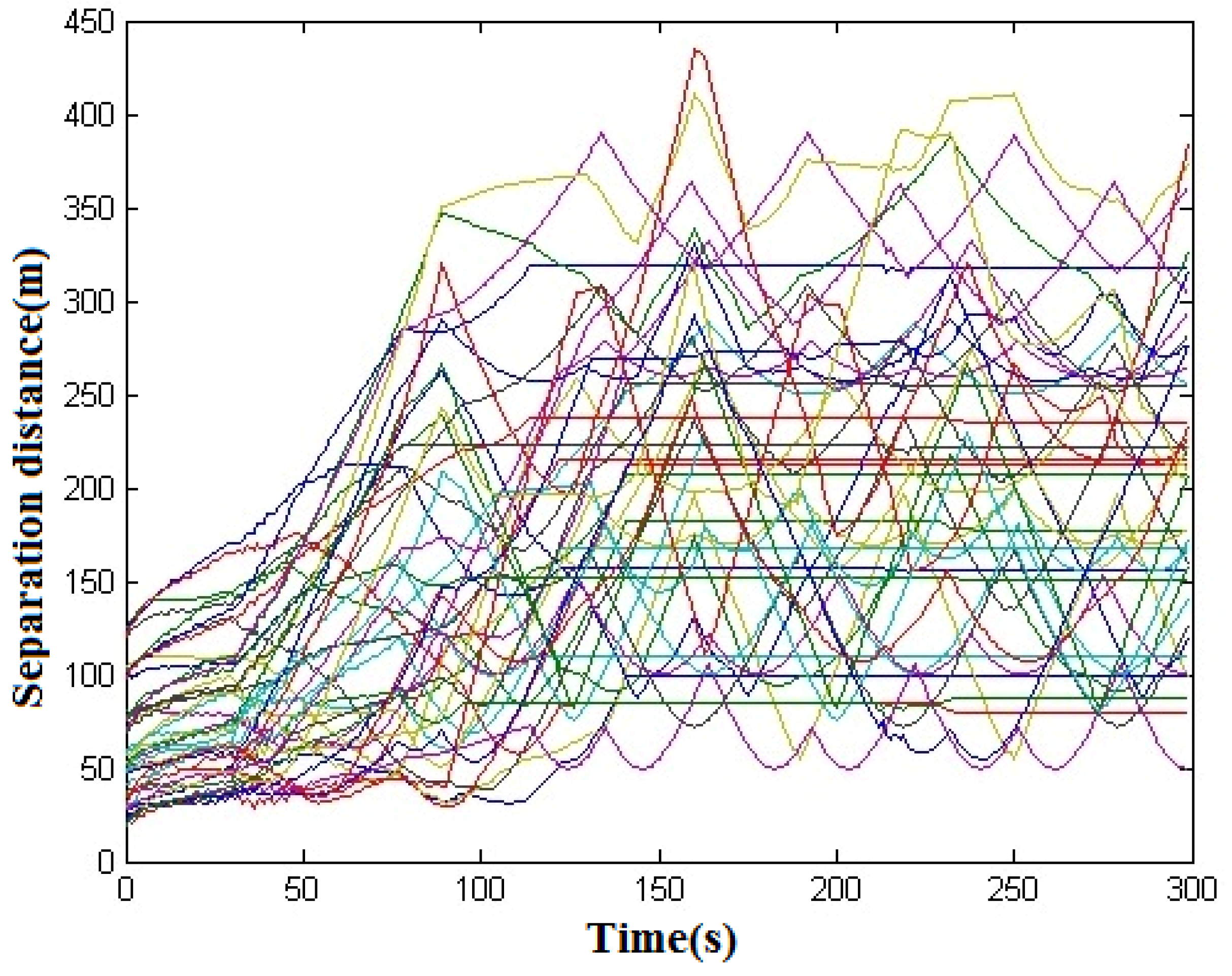
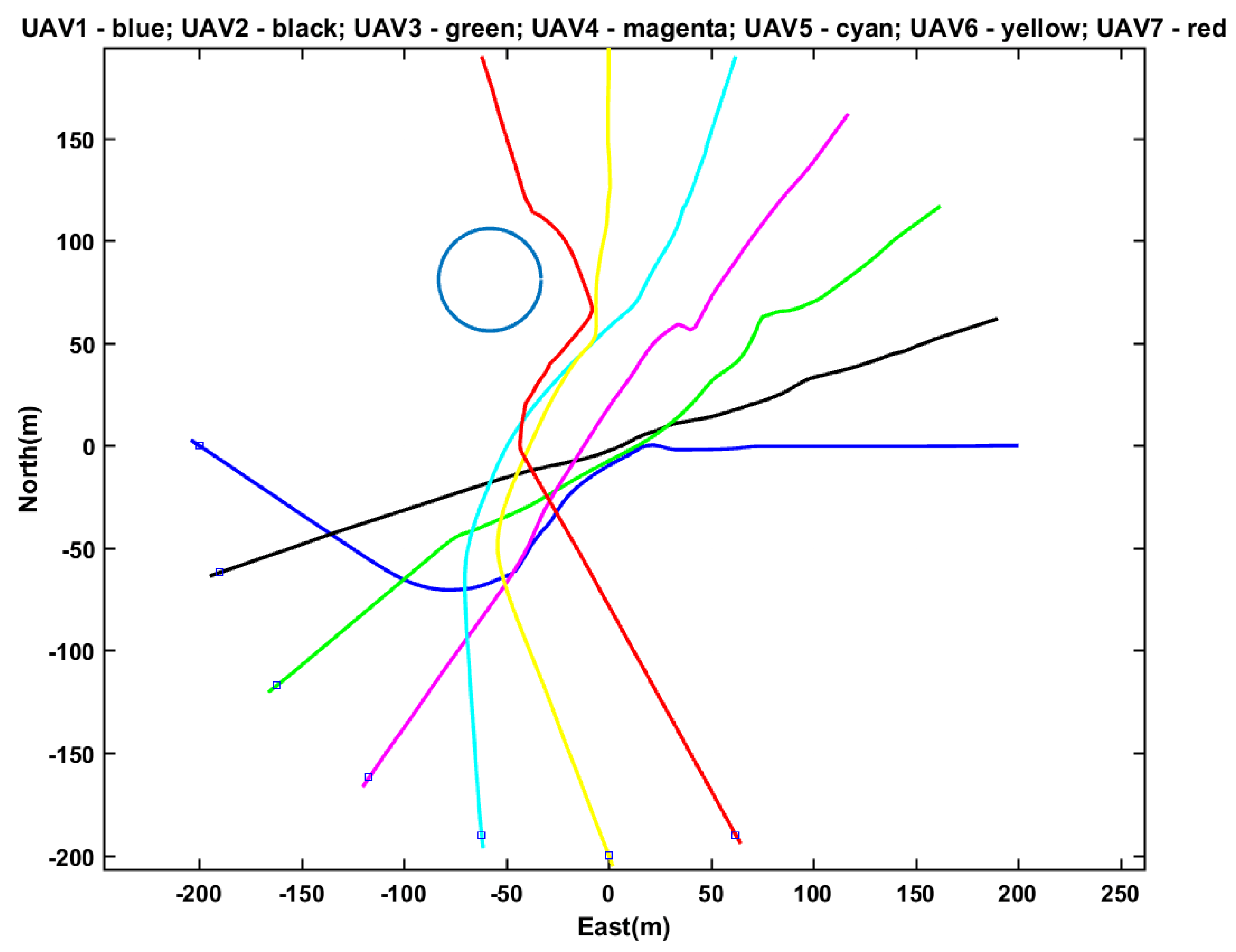
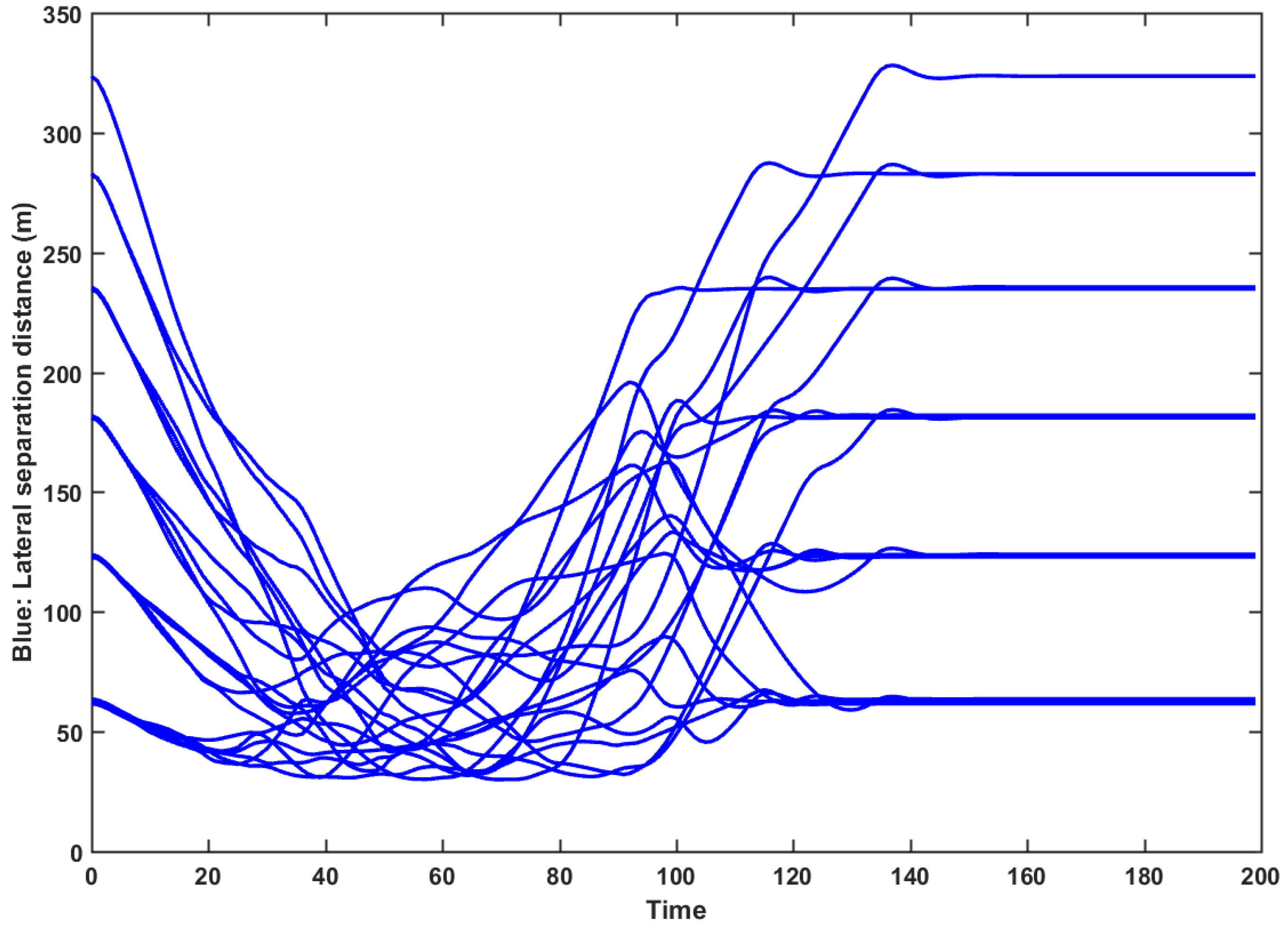
Case 4: Avoiding Moving Vehicles and a Static Obstacle. Consider a scenario with seven UAVs in the working area. Table 6 shows the initial coordinates and target assignment for each UAV. The maximum distance from the UAV for considering collision is 75 m. During this simulation, seven UAVs were within 75 m of each other in order to fully test the collision avoidance with all seven UAVs. The safe distance for the collision avoidance algorithm was set to 15 m, while the maximum speed of the UAV was set at 5 m/s. During this simulation, seven UAVs passed one circular obstacle and passed each other in order to test the collision avoidance algorithm against dynamical UAVs and a static obstacle. The flight paths are shown in Figure 20, while the horizontal distance profile (between the i-th UAV and j-th UAV) is shown in Figure 21. It was observed that the minimum separation distance was about 25 m. Thus, safety was maintained with the proposed collision avoidance algorithm.
This case was used to examine the proposed distributed collision avoidance control for MUAVS. In this form, all vehicles were connected with each other through communications, even when we considered a maximum range of only 75 m, as explained in Section 3.3.1 This implies that if one vehicle is far away from another (i.e., farther than 75 m), it will not affect the collision avoidance action of the vehicle. This solves the scalability issue when the number of vehicles increases. It was observed from the simulation that each vehicle only avoided the moving obstacles when it was near the obstacles (i.e., less than 75 m).
These case studies give a basic test for the proposed algorithm. Further analysis is necessary to validate the effectiveness in more stressful conditions (e.g., Monte Carlo simulation).
5. Hardware-in-the-Loop Simulation
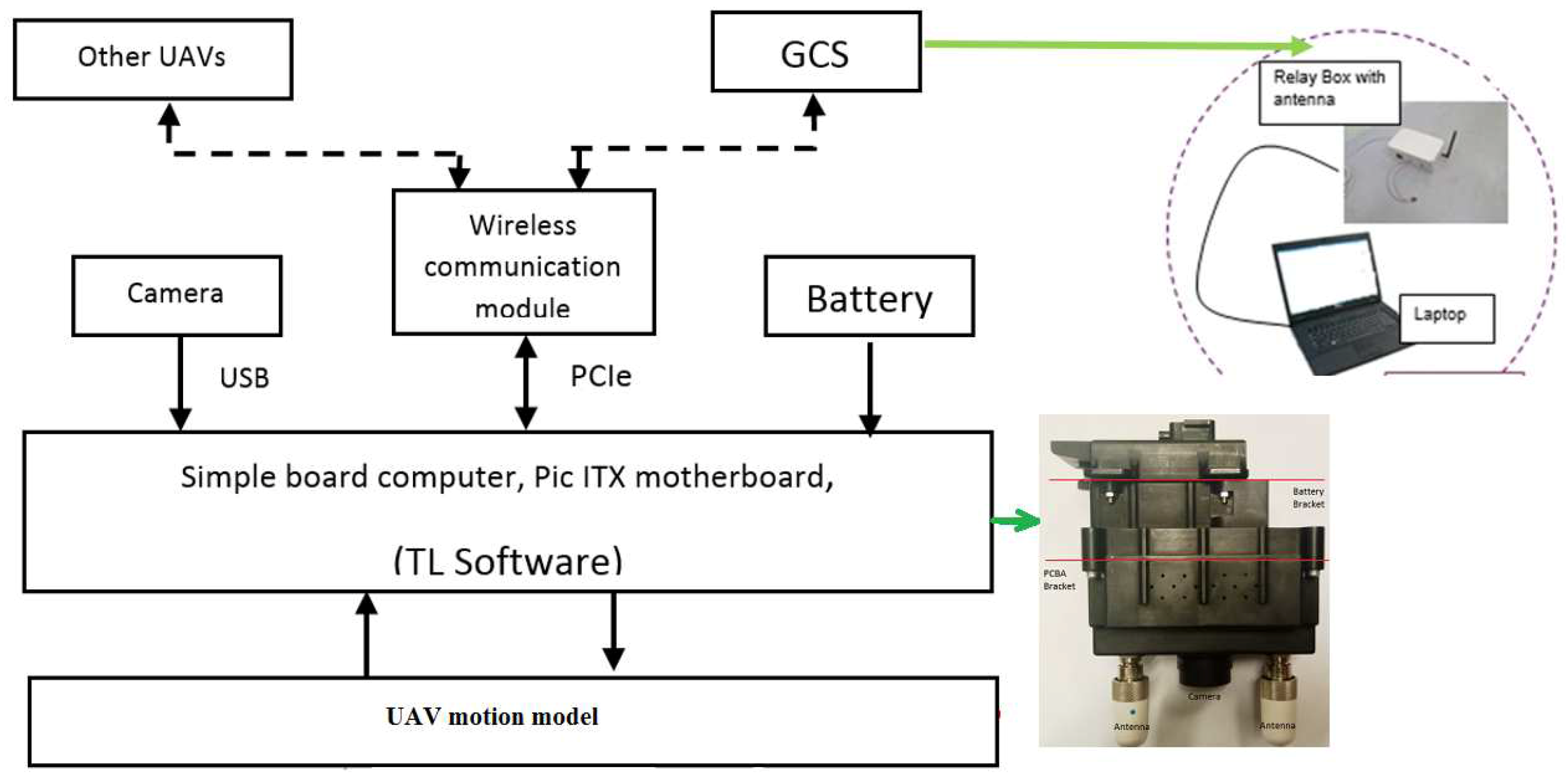
Hardware-in-the-loop simulation (HILS) is a type of real-time simulation. We wanted to use HILS to test the extreme case, the scenario is a cross between two groups of UAVs, which is difficult to do in a real flight test. Each UAV is composed of a hardware payload with a mathematical motion model in HILS (see Figure 22 and Table 7), and thus can communicate with the ground control station (GCS) and other UAVs. The HB exchange is achieved in UDP mode. In this way, each UAV can implement the distributed control based on the information obtained from the HB exchange. The motion model is given by:
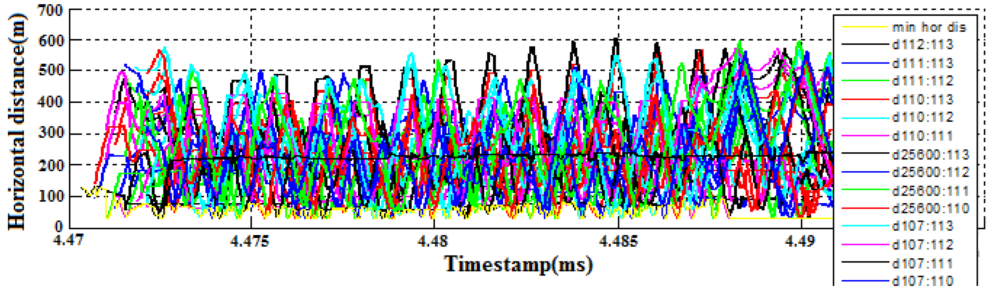
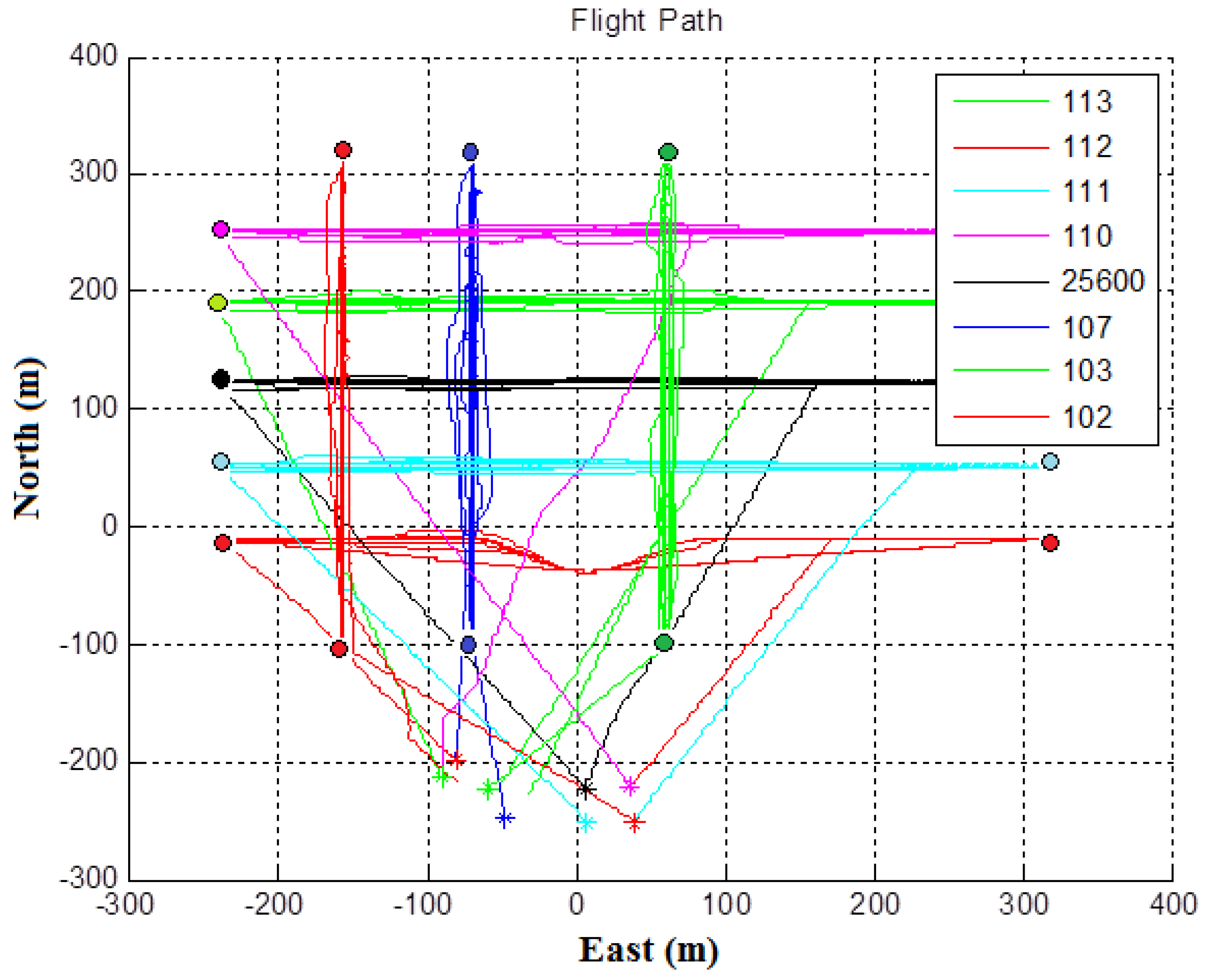
where T is the sampling time, and obtained from the VO algorithm are the velocity control signals along the directions, respectively. The motion model was used to generate the position and velocity of the UAV. Each UAV had a safe radius of 15 m. The GCS was used to broadcast the parameters (including target waypoints) of UAV control, launch, and recovery commands. Every UAV broadcasted its HB regularly at 1 Hz, while the position and velocity of UAVs were sampled at 10 Hz and the output to the UAV motion model by sending the velocity command was at the rate of 4 Hz. First, all UAVs were launched by a GCS launch command, climbing up vertically at an altitude of 60 m. Then, five UAVs (UAV IDs 113, 112, 110, 111, and 25600) went to the target waypoints to do patrol motion control from west to east and from east to west (along the x-axis), while three UAVs (UAV IDs 102, 103, and 107) went to the target waypoints do patrol motion control from south to north and from north to south (along the y-axis). Later, all UAVs were commanded to go back by the GCS. Finally, all UAVs landed at the launch points successfully. The flight paths of the eight UAVs are shown in Figure 23, while the separation distance profile between UAV to UAV along the horizontal direction is shown in Figure 24. It was observed that the minimum separation distance was about 30 m. This verifies that the VO algorithm was successful.
6. Conclusions
This paper presented a collision avoidance scheme for a multi-UAV system. We described a distributed cooperative control strategy through shared UAV messages and information fusion. This is a key point in our paper. By sharing HB information, each UAV knows the status of nearby UAVs and chooses a feasible velocity command to avoid collision with the obstacles. We also proposed an avoidance control approach dealing with polygonal obstacles. The core of this approach is to find the maximum angle of each half-space of the collision cone which is formed by the line between the vehicle and centroid of the polygonal obstacle. Simulation and hardware-in-the-loop tests verified that the algorithm can avoid static obstacles and moving UAVs. The drawback of the proposed algorithm is that the solution is locally optimal. In future research, we will have three jobs: incorporating the visibility graph algorithm to find a globally optimal path for improving the collision avoidance algorithm, investigating how uncertainties in GPS errors affect the performance of the collision avoidance algorithm and improving the algorithm accordingly, and comparing our algorithms with existing collision avoidance methods.
Author Contributions
S.H. designed heartbeats and avoiding polygonal obstacle method; R.S.H.T. designed the collision avoidance algorithm; W.L. was involved in the discussion and modification of the collision avoidance algorithm.
Funding
This research received no external funding.
Conflicts of Interest
The authors declare no conflict of interest.
Appendix A
Appendix B
Proof of Theorem 2.
First, we have to consider the braking time , which is how much time is required for a UAV to come to a full stop before colliding with another UAV. The worst case is that when the UAV finds that it is possible to have a collision with an obstacle, it takes a maximum deceleration b to brake down from its current velocity to a complete stop, that is, at time . Thus, it follows that
The braking time is obtained, that is
Second, the sliding distance during the time is
Third, at the same time, we also have to consider the obstacle moving at the speed at the worst case during that time . The moving distance is
Finally, the safe distance is given by
□
References
- Dalamagkidis, K.; Valavanis, K.P.; Piegl, L.A. On Integrating Unmanned Aircraft Systems into the National Airspace System, International Series on Intelligent Systems, Control, and Automation: Science and Engineering; Springer: New York, NY, USA, 2009; Volume 54, pp. 43–59. [Google Scholar]
- Lozano-Prez, T.; Wesley, M.A. An algorithm for planning collision-free paths among polyhedral obstacles. Commun. ACM 1979, 22, 560–570. [Google Scholar] [CrossRef]
- Borenstein, J.; Koren, Y. The vector field histogram-fast obstacle avoidance for mobile robots. IEEE Trans. Robot. Autom. 1991, 7, 278–288. [Google Scholar] [CrossRef] [Green Version]
- Minguez, J.; Montano, L. Nearness diagram (ND) navigation: Collision avoidance in troublesome scenarios. IEEE Trans. Robot. Autom. 2004, 20, 45–49. [Google Scholar] [CrossRef]
- Bellingham, J.; Tillerson, M.; Richards, A.; How, J.P. Multi-Task Allocation and Path Planning for Cooperating UAVs, Chapter 2. In Cooperative Control: Models, Applications and Algorithms; Butenko, S., Murphey, R., Pardalos, P.M., Eds.; Springer Science + Business Media: Berlin, Germany, 2003. [Google Scholar]
- Watanabe, Y.; Calise, A.; Johnson, E.; Evers, J. Minimum-Effort Guidance for Vision-Based Collision Avoidance. In Proceedings of the AIAA Atmospheric Flight Mechanics Conference and Exhibit, Honolulu, HI, USA, 21–24 August 2006. [Google Scholar]
- Mujumdar, A.; Padhi, R. Reactive Collision Avoidance of Using Nonlinear Geometric and Differential Geometric Guidance. J. Guid. Control Dyn. 2012, 34, 303–311. [Google Scholar] [CrossRef]
- Nikolos, I.; Valavanis, K.; Tsourveloudis, N.; Kostaras, A. Evolutionary Algorithm Based Offline/Online Path Planner for UAV Navigation. IEEE Trans. Syst. Man Cybern. Part B Cybern. 2003, 33, 898–912. [Google Scholar] [CrossRef] [PubMed]
- Borrelli, F.; Subramanian, D.; Raghunathan, A.; Biegler, L. MILP and NLP Techniques for Centralized Trajectory Planning of Multiple Unmanned AirVehicles. In Proceedings of the American Control Conference, Piscataway, NJ, USA, 14–16 June 2006; Volume 2006, pp. 5763–5768. [Google Scholar]
- Kochenderfer, M.J.; Holland, J.E.; Chryssanthacopoulos, J.P. Next Generation Airborne Collision Avoidance System. Lincoln Lab. J. 2012, 19, 55–71. [Google Scholar]
- Cosio, F.A.; Castaneda, M.P. Autonomous Robot Navigation Using Adaptive Potential Fields. Math. Comput. Model. 2004, 40, 1141–1156. [Google Scholar] [CrossRef]
- Fiorini, P.; Shiller, Z. Motion Planning in Dynamic Environments Using Velocity Obstacles. Int. J. Robot. Res. 1998, 17, 760–772. [Google Scholar] [CrossRef] [Green Version]
- Van den Berg, J.; Guy, S.; Lin, M.; Manocha, D. Reciprocal n-body collision avoidance. In Robotics Research: the 14th International Symposium ISRR, Number 70 in Springer Tracts in Advanced Robotics; Pradalier, C., Siegwart, R., Hirzinger, G., Eds.; Springer: Berlin/Heidelberg, Germany, 2011; pp. 3–19. [Google Scholar]
- Kluge, B.; Prassler, E. Recursive Probabilistic Velocity Obstacles for Reflective Navigation. In Field and Service Robotics; Yuta, S., Asama, H., Prassler, E., Tsubouchi, T., Thrun, S., Eds.; Springer Tracts in Advanced Robotics; Springer: Berlin/Heidelberg, Germany, 2006; Volume 24, pp. 71–79. [Google Scholar]
- Snape, J.; van den Berg, J.; Guy, S.; Manocha, D. The Hybrid Reciprocal Velocity Obstacle. IEEE Trans. Robot. 2011, 27, 696–706. [Google Scholar] [CrossRef] [Green Version]
- Conroy, P.; Bareiss, D.; Beall, M.; van den Berg, J. 3-D reciprocal collision avoidance on physical quadrotor helicopters with on-board sensing for relative positioning. arXiv, 2014; arXiv:1411.3794. [Google Scholar]
- Allawi, Z.T.; Abdalla, T.Y. An ABC-optimized reciprocal velocity obstacle algorithm for navigation of multiple mobile robots. In Proceedings of the Second Engineering Conference of Control, Computers Mechatronics Engineering, Baghdad, Iraq, 25–27 February 2014; pp. 231–238. [Google Scholar]
- Huang, S.; Teo, R.S.H.; Liu, W.; Dymkou, S.M. Distributed Cooperative Collision Avoidance Control and Implementation for Multi-Unmanned Aerial Vehicles. In Proceedings of the 2017 Asian Control Conference, Gold Coast, Australia, 17–20 December 2017. [Google Scholar]
- Pallottino, L.; Scordio, V.G.; Bicchi, A.; Frazzoli, E. Decentralized Cooperative Policy for Conflict Resolution in Multivehicle Systems. IEEE Trans. Robot. 2007, 23, 1170–1183. [Google Scholar] [CrossRef]
- Chakravarthy, A.; Ghose, D. Obstacle Avoidance in a Dynamic Environment: A Collision Cone Approach. IEEE Trans. Syst. Man Cybern. Part A Syst. Hum. 1998, 28, 562–574. [Google Scholar] [CrossRef]
- Jenie, Y.I.; Kampen, E.-J.V.; de Visser, C.C.; Chu, Q.P. Velocity Obstacle Method for Non-cooperative autonomous collision avoidance systems for UAVs. In Proceedings of the AIAA Guidance, Navigation, and Control Conference, National Harbor, MD, USA, 13–17 January 2014; pp. 1–12. [Google Scholar]
- Kuwata, Y.; Wolf, M.T.; Zarzhitsky, D.; Huntsberger, T.L. Safe maritime navigation with COLREGS using velocity obstacles. In Proceedings of the IEEE/RSJ International Conference on Intelligent Robots and Systems (IROS11), San Francisco, CA, USA, 25–30 September 2011; pp. 4728–4734. [Google Scholar]
- Jenie, Y.I.; Kampen, E.-J.V.; de Visser, C.C.; Ellerbroek, J.; Hoekstra, J.M. Selective Velocity Obstacle Method for Deconflicting ManeuversApplied to Unmanned AerialVehicles. J. Guid. Control Dyn. 2015, 38, 1140–1146. [Google Scholar] [CrossRef]
- Van der Berg, J.; Lin, M.; Manocha, D. Reciprocal Velocity Obstacles for Real-Time Multi-Agent Navigation. In Proceedings of the 2008 IEEE International Conference on Robotics and Automation (ICRA), Piscataway, NJ, USA, 19–23 May 2008; pp. 1928–1935. [Google Scholar]
- Roelofsen, S.; Gillet, D.; Martinoli, A. Collision Avoidance with Limited Field of View Sensing: A Velocity Obstacle Approach. In Proceedings of the 2017 IEEE International Conference on Robotics and Automation (ICRA), Singapore, 29 May–3 June 2017; pp. 1922–1927. [Google Scholar]
- Kurose, J.F.; Ross, K.W. Computer Networking: A Top-Down Approach, 6th ed.; Pearson Education: Boston, MA, USA, 2010; pp. 157–162. [Google Scholar]
- Tsourdos, A.; White, B.; Shanmugavel, M. Cooperative Path Planning of Unmanned Aerial Vehicles; John Wiley & Sons: Chichester, UK, 2011. [Google Scholar]
Figure 1.
Information fusion. HB: heartbeat.
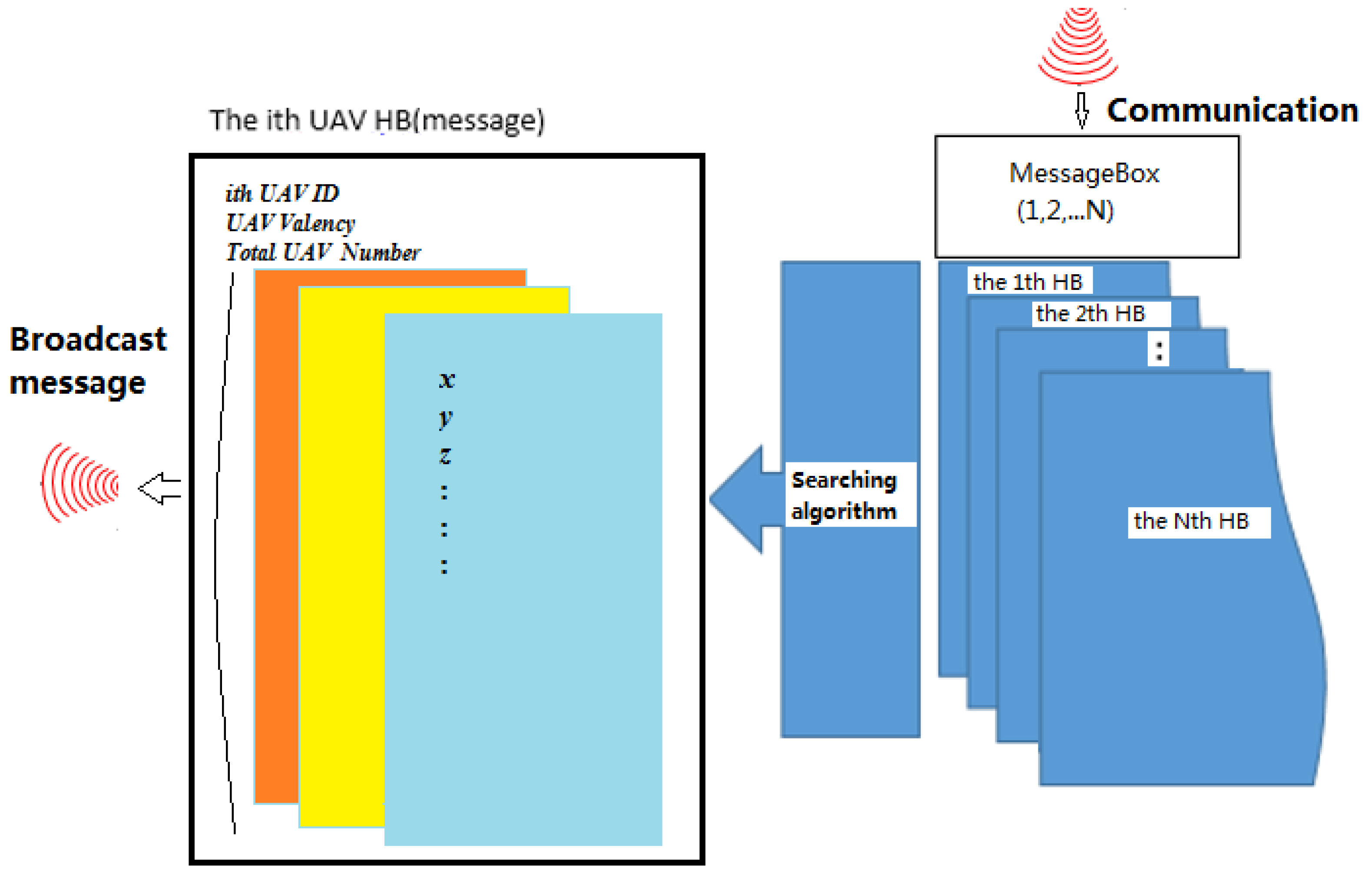
Figure 2.
Weakly connected network: Three cases are shown in (a) tree form, (b) ring form, and (c) line form.
Figure 2.
Weakly connected network: Three cases are shown in (a) tree form, (b) ring form, and (c) line form.
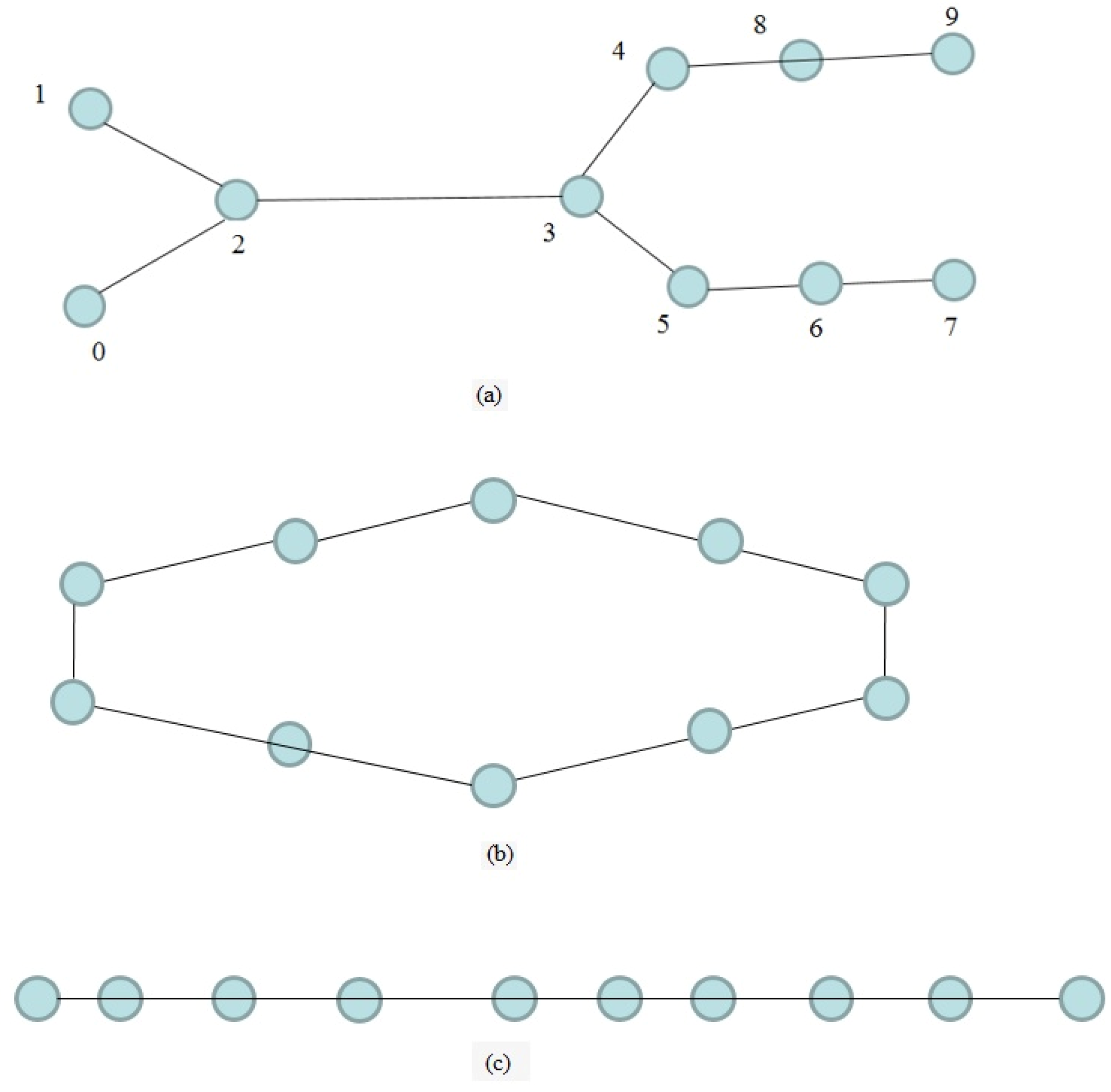
Figure 3.
UAVs performing collision avoidance cooperatively through shared HB.

Figure 4.
UAV control with collision avoidance algorithm.
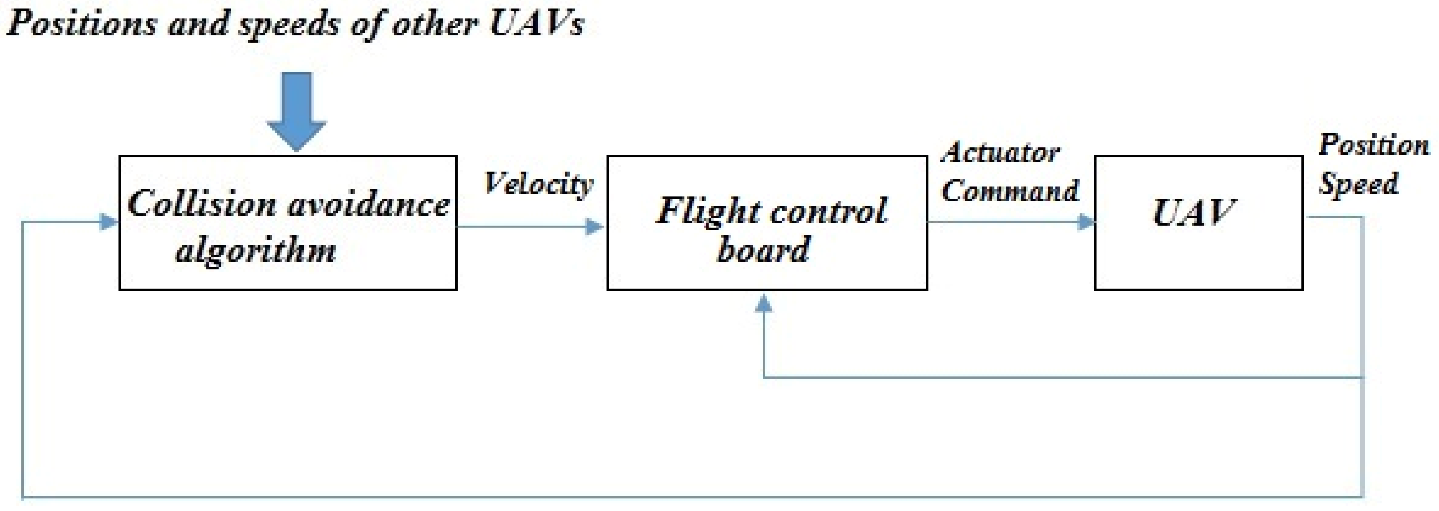
Figure 5.
Maximum range around vehicle A: Vehicles B, C, D, and E are within vehicle A’s range.

Figure 6.
Velocity obstacles. There are two vehicles A and B with the respective radii and at the respective positions and . and are the velocity vectors of vehicles A and B respectively. The light cone represents the velocity obstacle on vehicle A if vehicle B was stationary. The dark cone denoted as represents the same velocity obstacle when taking into account vehicle B’s velocity .
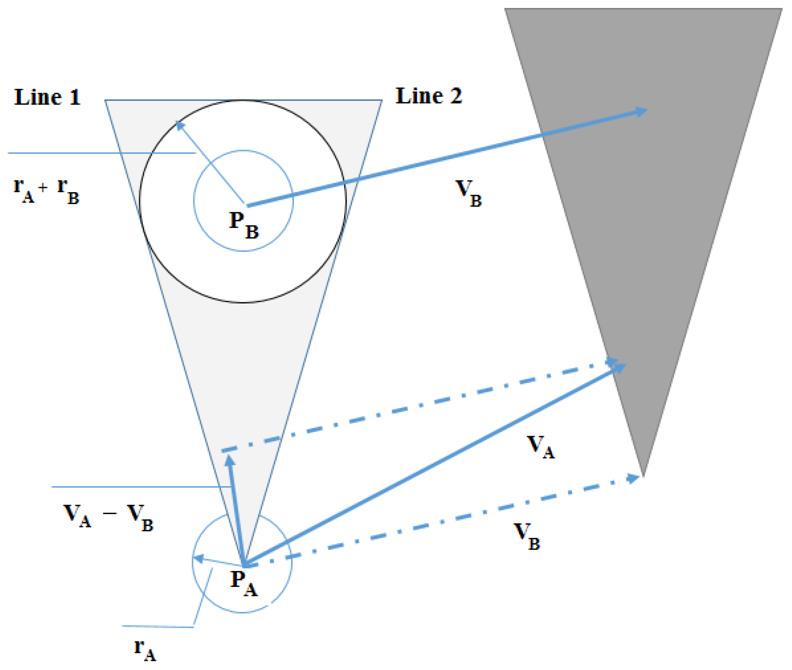
Figure 7.
Vehicle A considers vehicle B as an obstacle. It shows that vehicle A has three regions, , , and , around the velocity obstacle.
Figure 7.
Vehicle A considers vehicle B as an obstacle. It shows that vehicle A has three regions, , , and , around the velocity obstacle.

Figure 8.
Rules of the sea, COLREGS. The rule is essentially about passing on the right side of other traffic.
Figure 8.
Rules of the sea, COLREGS. The rule is essentially about passing on the right side of other traffic.
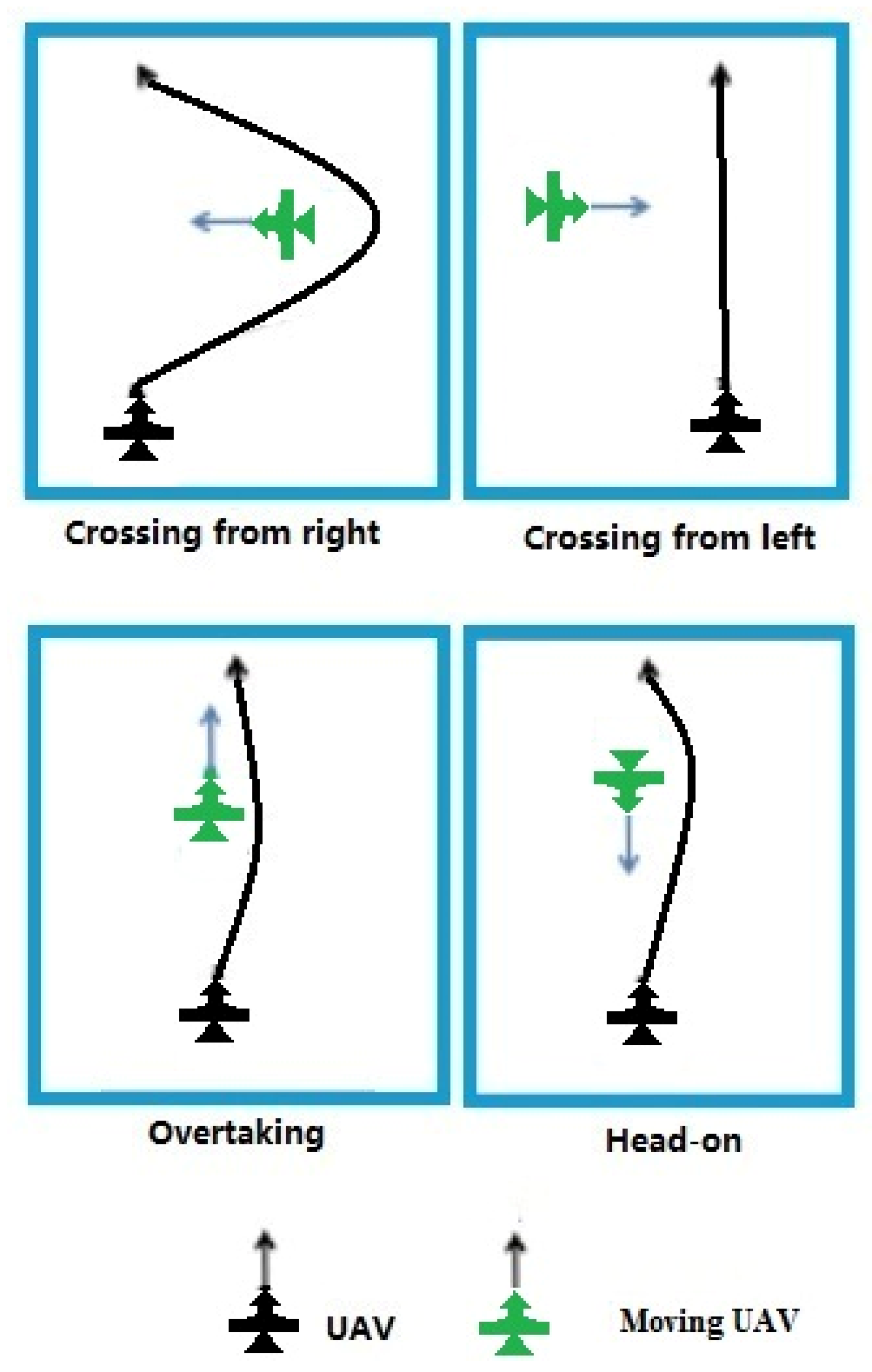
Figure 9.
The velocity obstacle associated with a static circular obstacle. There is one vehicle A and one obstacle B with the respective radii and at the respective positions and . Vehicle A will touch the perimeter around obstacle B in time if using the command speed . At this moment, vehicle A’s position is at .

Figure 10.
Non-convex polygon divided into convex polygons.
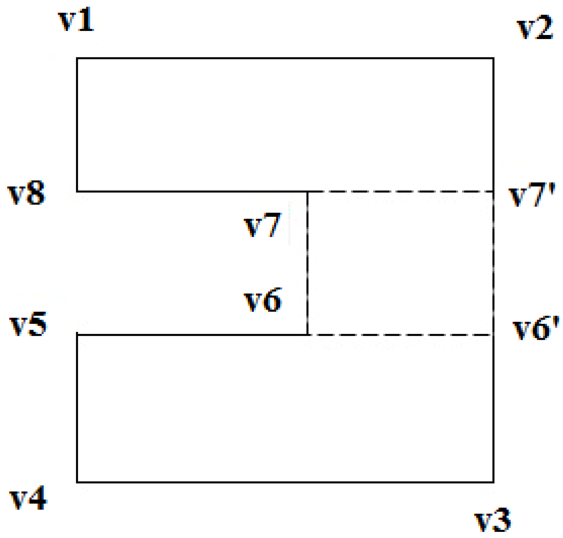
Figure 11.
Polygon expansion: R is safe constant width.

Figure 12.
Vehicle A at position faces one polygonal obstacle B. The centroid of the polygon is at . The vector pass through and .
Figure 12.
Vehicle A at position faces one polygonal obstacle B. The centroid of the polygon is at . The vector pass through and .
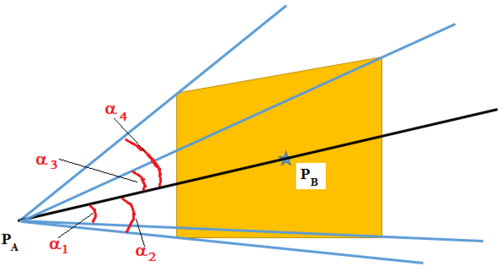
Figure 13.
Case 1: Cooperative collision avoidance against static circle obstacle. Symbols “i,pj” represent the ith UAV with priority level (j = 1 at low priority; j = 3 at high priority).
Figure 13.
Case 1: Cooperative collision avoidance against static circle obstacle. Symbols “i,pj” represent the ith UAV with priority level (j = 1 at low priority; j = 3 at high priority).

Figure 14.
Test 1: Separation distance along horizontal direction.

Figure 15.
Case 2: Cooperative collision avoidance against polygonal obstacle. Symbols “i,pj” represent the ith UAV with priority level (j = 1 at low priority; j = 3 at high priority).
Figure 15.
Case 2: Cooperative collision avoidance against polygonal obstacle. Symbols “i,pj” represent the ith UAV with priority level (j = 1 at low priority; j = 3 at high priority).
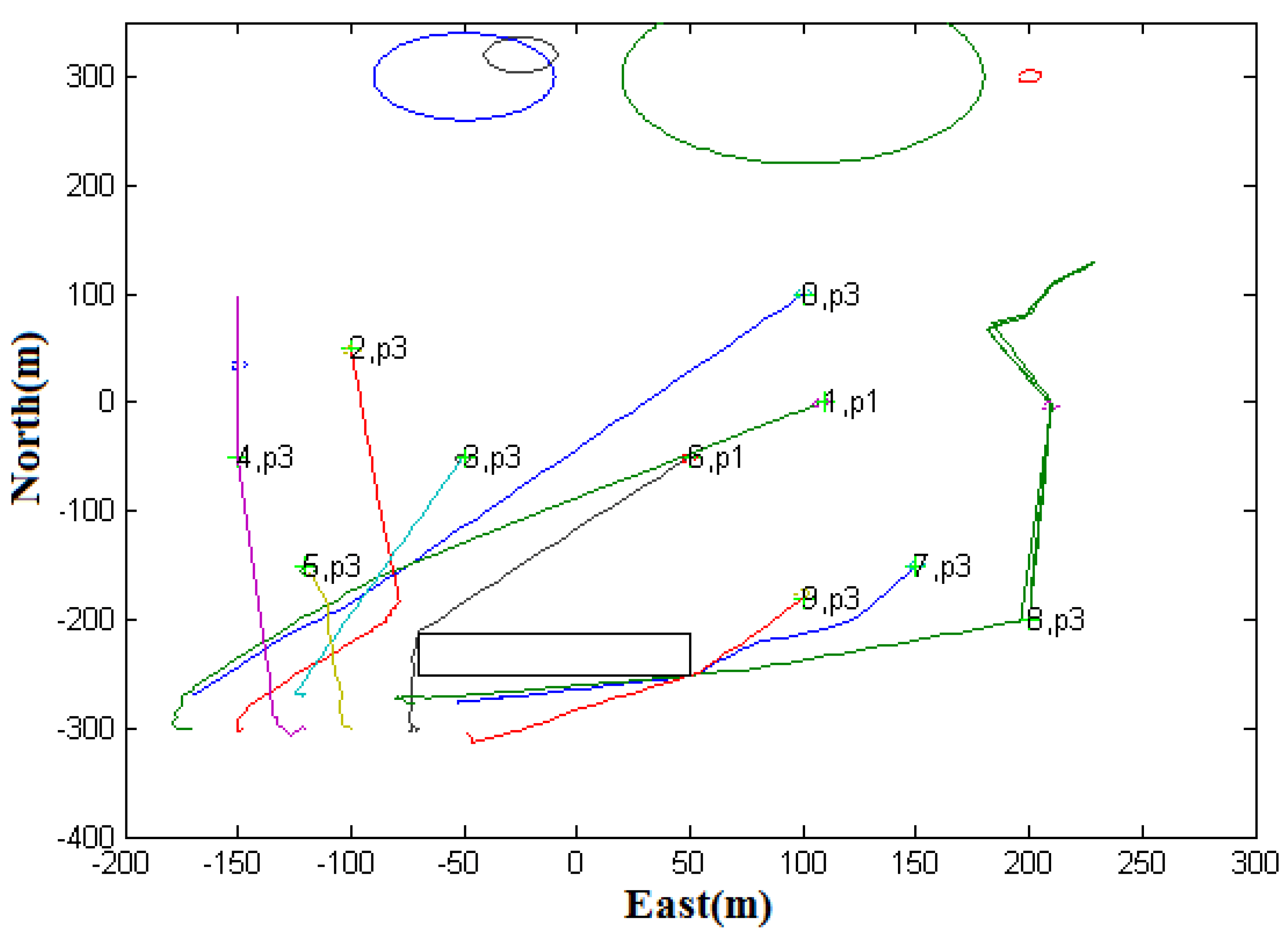
Figure 16.
Case 3: Cooperative collision avoidance against temporary communication failure (normal situation): UAVs 1 and 0 perform collision avoidance.
Figure 16.
Case 3: Cooperative collision avoidance against temporary communication failure (normal situation): UAVs 1 and 0 perform collision avoidance.
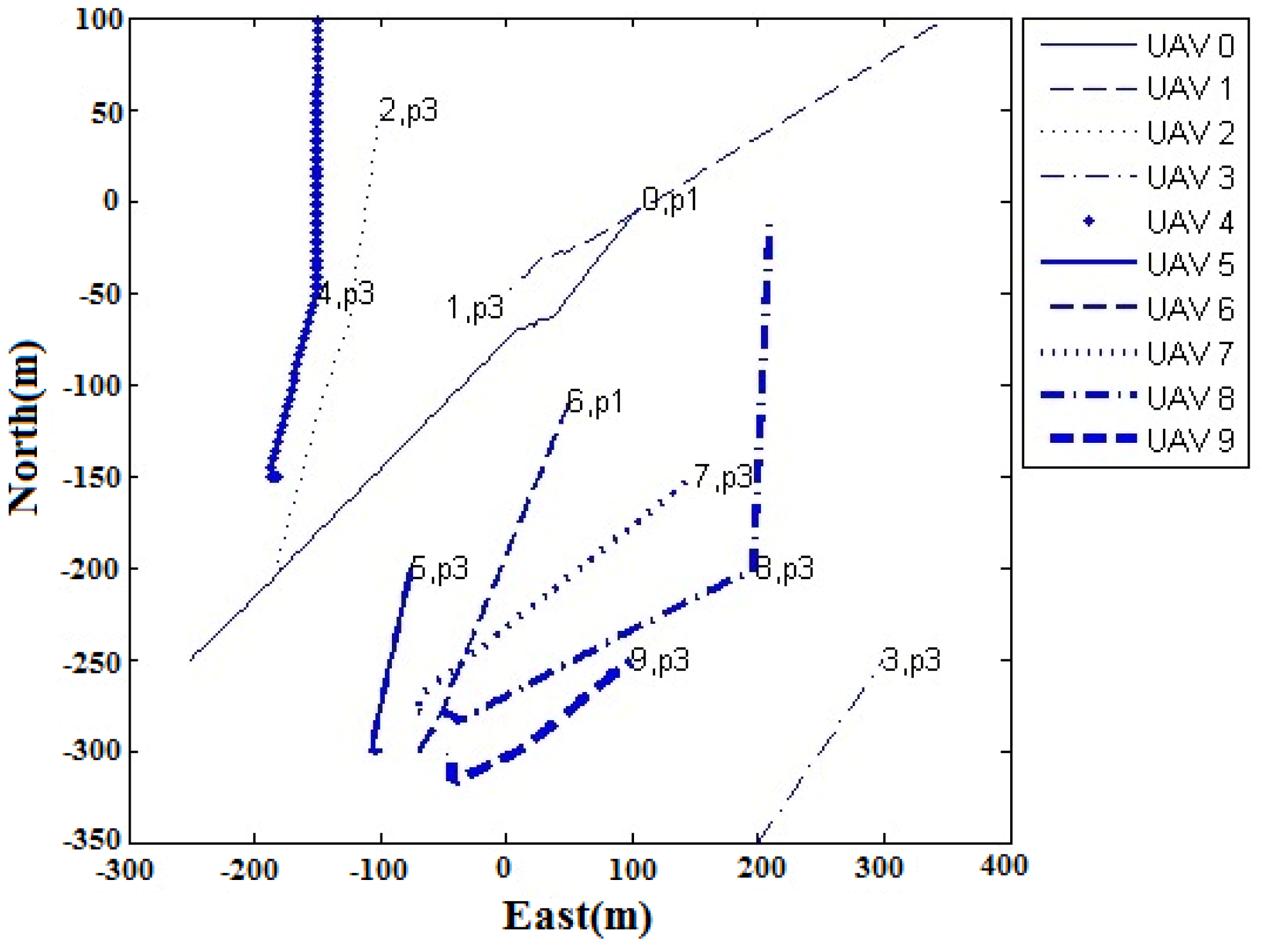
Figure 17.
Case 3: Cooperative collision avoidance against temporary communication failure (normal situation): Separation distance along the horizontal direction.
Figure 17.
Case 3: Cooperative collision avoidance against temporary communication failure (normal situation): Separation distance along the horizontal direction.

Figure 18.
Case 3: Cooperative collision avoidance against temporary communication failure (unhealthy situation): Red star represents temporary communication failure at time 75 s, and UAVs 1 and 0 perform collision avoidance.
Figure 18.
Case 3: Cooperative collision avoidance against temporary communication failure (unhealthy situation): Red star represents temporary communication failure at time 75 s, and UAVs 1 and 0 perform collision avoidance.
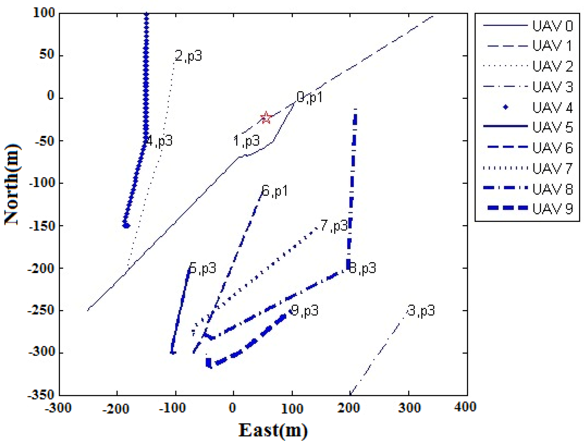
Figure 19.
Case 3: Cooperative collision avoidance against temporary communication failure (unhealthy situation): Separation distance along horizontal direction.
Figure 19.
Case 3: Cooperative collision avoidance against temporary communication failure (unhealthy situation): Separation distance along horizontal direction.
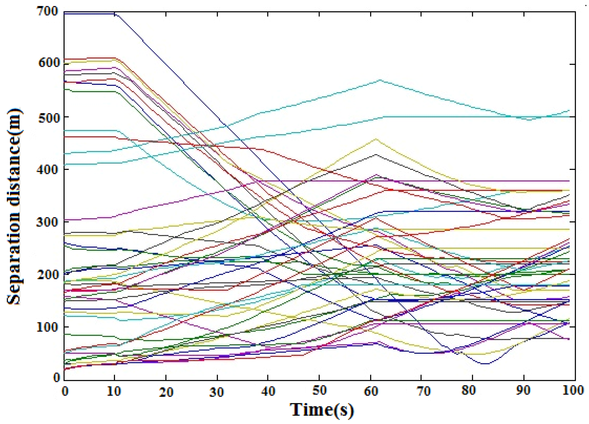
Figure 20.
Case 4: Seven UAV control (flight paths).

Figure 21.
Case 4: Seven UAV control (horizontal separation distance profile).

Figure 22.
Hardware-in-the-loop simulation (HILS): Payload. GCS: ground control station.

Figure 23.
HILS: Patrol motion control of eight UAVs: stars represent launching points and recovery points, circles represent target waypoints.
Figure 23.
HILS: Patrol motion control of eight UAVs: stars represent launching points and recovery points, circles represent target waypoints.

Figure 24.
HILS: Separation distance from UAV to UAV.

Table 1.
Limitations of existing velocity obstacle methods.
| Reference | Suitability for MUAVs | Robust to Communication Failure | Cooperation | Low Computational Cost | Polygonal Obstacle |
|---|---|---|---|---|---|
| [20] | No | Yes | No | No | Yes |
| [12] | Yes | No | Yes | No | No |
| [22] | No | Yes | No | No | No |
| [23] | Yes | No | Yes | Yes | No |
| [21] | No | Yes | No | Yes | No |
| [14] | Yes | No | Yes | No | No |
| [13,24] | No | No | Yes | No | No |
| [16] | No | Yes | No | No | No |
| [17] | No | Yes | No | Yes | No |
| [15] | No | No | Yes | No | No |
| [25] | No | No | Yes | No | No |
Table 2.
Unmanned aerial vehicle (UAV) () heartbeat.
| UAV ID |
| UAV adjacent number (UAV valency) |
| Total UAV number in network |
| x position |
| y position |
| z position |
| speed |
| speed |
| speed |
| GPS time |
| UAV mode |
| Replacement UAV |
| Target ID |
| Want to target ID |
| Cost |
| UAV status |
Table 3.
Simulation of collision avoidance of MUAVS: Case 1.
| UAV ID | Initial Coordinates (N,E) | Target Waypoints (N,E) |
|---|---|---|
| UAV 0 | (−270, −170) | (100, 100) |
| UAV 1 | (−300, −170) | (0, 110) |
| UAV 2 | (−300, −150) | (50, −100) |
| UAV 3 | (−270, −120) | (−50, −50) |
| UAV 4 | (−300, −120) | (−50, −120)–(100,−50) |
| UAV 5 | (−300, −100) | (−150, −120)–(−150, 70) |
| UAV 6 | (−300, −70) | (120, 50)–(120, −100) |
| UAV 7 | (−280, −50) | (−150, 150) |
| UAV 8 | (−280, −70) | (−200, −200)–(0, 210)–(70, 180)–(80, 200)–(110, 210)–(130, 230) |
| UAV 9 | (−300, −50) | (−70, 100) |
Table 4.
Simulation of collision avoidance of MUAVS: Case 2.
| UAV ID | Initial Coordinates (N,E) | Target Waypoints (N,E) |
|---|---|---|
| UAV 0 | (−270, −170) | (100, 100) |
| UAV 1 | (−300, −170) | (0, 110) |
| UAV 2 | (−300, −150) | (50, −100) |
| UAV 3 | (−270, −120) | (−50, −50) |
| UAV 4 | (−300, −120) | (−50, −150)–(100, −150) |
| UAV 5 | (−300, −100) | (−150, −120) |
| UAV 6 | (−300, −70) | (−50, 50) |
| UAV 7 | (−280, −50) | (−150, 150) |
| UAV 8 | (−280, −70) | (−200, −200)–(0, 210)–(70, 180)–(80, 200)–(110, 210)–(130, 230) |
| UAV 9 | (−300, −50) | (−180, 100) |
Table 5.
Simulation of collision avoidance of MUAVS: Case 3.
| UAV ID | Initial Coordinates (N,E) | Target Waypoints (N,E) |
|---|---|---|
| UAV 0 | (−250, −250) | (1, 110) |
| UAV 1 | (100, 350) | (−50, 0) |
| UAV 2 | (−200, −180) | (50, −100) |
| UAV 3 | (−350, 200) | (−250, 300) |
| UAV 4 | (−150, −180) | (−50, −150)–(100, −150) |
| UAV 5 | (−300, −100) | (−200, −75) |
| UAV 6 | (−300, −70) | (−110, 50) |
| UAV 7 | (−280, −70) | (−150, 150) |
| UAV 8 | (−280, −50) | (−200, 200)–(0, 210) |
| UAV 9 | (−300, −50) | (−250, 100) |
Table 6.
Simulation of collision avoidance of MUAVS: Case 4.
| UAV ID | Initial Coordinates (N,E) | Target Waypoints (N,E) |
|---|---|---|
| UAV 1 | (0, 200) | (0, −200) |
| UAV 2 | (62, 190) | (−62, −190) |
| UAV 3 | (117, 162) | (−117, −162) |
| UAV 4 | (162, 117) | (−162, −117) |
| UAV 5 | (192, 62) | (−192, −62) |
| UAV 6 | (200, 0) | (−200, 0) |
| UAV 7 | (190, −62) | (−190, 62) |
Table 7.
Hardware components in payload.
| Components | Company | Model Number | Description |
|---|---|---|---|
| Single-Board Computer | Commell | LP173E | 1.91 GHz quad core processor |
| Network Interface Card | Mikrotik | R11e-5HnD | Mini PCIe, 802.11a/n |
| Camera | E-con system | See3CAM_11CUG | 1.3 MP |
| Antenna | Cisco | AIR-ANT5135SDW | 3.5 dBi, 5150–5850 MHz |
| Battery | AA Portable Power Corp | ICR18650B4 | 3-cell 11.1 V 2600 mAh |
© 2018 by the authors. Licensee MDPI, Basel, Switzerland. This article is an open access article distributed under the terms and conditions of the Creative Commons Attribution (CC BY) license (http://creativecommons.org/licenses/by/4.0/).
Share and Cite
MDPI and ACS Style
Huang, S.; Teo, R.S.H.; Liu, W. Distributed Cooperative Avoidance Control for Multi-Unmanned Aerial Vehicles. Actuators 2019, 8, 1. https://doi.org/10.3390/act8010001
AMA Style
Huang S, Teo RSH, Liu W. Distributed Cooperative Avoidance Control for Multi-Unmanned Aerial Vehicles. Actuators. 2019; 8(1):1. https://doi.org/10.3390/act8010001
Chicago/Turabian StyleHuang, Sunan, Rodney Swee Huat Teo, and Wenqi Liu. 2019. "Distributed Cooperative Avoidance Control for Multi-Unmanned Aerial Vehicles" Actuators 8, no. 1: 1. https://doi.org/10.3390/act8010001
Note that from the first issue of 2016, this journal uses article numbers instead of page numbers. See further details here.